Sturm 3-ball global attractors 2:
Design of Thom-Smale complexes

Abstract

This is the second of three papers on the geometric and combinatorial characterization of global Sturm attractors which consist of a single closed 3-ball. The underlying scalar PDE is parabolic,

$$u_{t}=u_{xx}+f(x,u,u_{x})\,,$$

on the unit interval $0<x<1$ with Neumann boundary conditions. Equilibria are assumed to be hyperbolic.

Geometrically, we study the resulting Thom-Smale dynamic complex with cells defined by the fast unstable manifolds of the equilibria. The Thom-Smale complex turns out to be a regular cell complex. Our geometric description involves a bipolar orientation of the 1-skeleton, a hemisphere decomposition of the boundary 2-sphere by two polar meridians, and a meridian overlap of certain 2-cell faces in opposite hemispheres.

The combinatorial description is in terms of the Sturm permutation, alias the meander properties of the shooting curve for the equilibrium ODE boundary value problem. It involves the relative positioning of extreme 2-dimensionally unstable equilibria at the Neumann boundaries $x=0$ and $x=1$, respectively, and the overlapping reach of polar serpents in the shooting meander.

In the first paper we showed the implications

$$\text{Sturm attractor}\quad\Longrightarrow\quad\text{Thom-Smale complex}\quad\Longrightarrow\quad\text{meander}\,.$$

The present part 2, closes the cycle of equivalences by the implication

$$\text{meander}\quad\Longrightarrow\quad\text{Sturm attractor}\,.$$

In particular this cycle allows us to construct a unique Sturm 3-ball attractor for any prescribed Thom-Smale complex which satisfies the geometric properties of the bipolar orientation and the hemisphere decomposition. Many explicit examples and illustrations will be discussed in part 3. The present 3-ball trilogy, however, is just another step towards the still elusive geometric and combinational characterization of all Sturm global attractors in arbitrary dimensions.

*
Institut für Mathematik
Freie Universität Berlin
Arnimallee 3
14195 Berlin, Germany

**
Center for Mathematical Analysis, Geometry and Dynamical Systems
Instituto Superior Técnico
Universidade de Lisboa
Avenida Rovisco Pais
1049–001 Lisbon, Portugal

1 Introduction

For a general introduction we first follow [FiRo16] and the references there. Sturm global attractors $\mathcal{A}_{f}$ are the global attractors of scalar parabolic equations

(1.1) $$u_{t}=u_{xx}+f(x,u,u_{x})$$

on the unit interval $0<x<1$. Just to be specific we consider Neumann boundary conditions $u_{x}=0$ at $x=0,1$. Standard semigroup theory provides local solutions $u(t,x)$ for $t\geq 0$ and given initial data at time $t=0$, in suitable Sobolev spaces $u(t,\cdot)\in X\subseteq C^{1}([0,1],\mathbb{R})$. Under suitable dissipativeness assumptions on $f\in C^{2}$, any solution eventually enters a fixed large ball in $X$. In fact that large ball of initial conditions itself limits onto the maximal compact and invariant subset $\mathcal{A}_{f}$ which is called the global attractor. See [He81, Pa83, Ta79] for a general PDE background, and [BaVi92, ChVi02, Edetal94, Ha88, Haetal02, La91, Ra02, SeYo02, Te88] for global attractors in general.

Equilibria $v=v(x)$ are time-independent solutions, of course, and hence satisfy the ODE

(1.2) $$0=v_{xx}+f(x,v,v_{x})$$

for $0\leq x\leq 1$, again with Neumann boundary. Here and below we assume that all equilibria $v$ of (1.1), (1.2) are hyperbolic, i.e. without eigenvalues (of) zero (real part) of their linearization. Let $\mathcal{E}=\mathcal{E}_{f}\subseteq\mathcal{A}_{f}$ denote the set of equilibria. Our generic hyperbolicity assumption and dissipativeness of $f$ imply that $N$:= $|\mathcal{E}_{f}|$ is odd.

It is known that (1.1) possesses a Lyapunov function, alias a variational or gradient-like structure, under separated boundary conditions; see [Ze68, Ma78, MaNa97, Hu11, Fietal14]. In particular, the global attractor consists of equilibria and of solutions $u(t,\cdot)$, $t\in\mathbb{R}$, with forward and backward limits, i.e.

(1.3) $$\underset{t\rightarrow-\infty}{\mathrm{lim}}u(t,\cdot)=v\,,\qquad\underset{t\rightarrow+\infty}{\mathrm{lim}}u(t,\cdot)=w\,.$$

In other words, the $\alpha$- and $\omega$-limit sets of $u(t,\cdot)$ are two distinct equilibria $v$ and $w$. We call $u(t,\cdot)$ a heteroclinic or connecting orbit, or instanton, and write $v\leadsto w$ for such heteroclinically connected equilibria.

We attach the name of Sturm to the PDE (1.1), and to its global attractor $\mathcal{A}_{f}$ because of a crucial nodal property of its solutions which we express by the zero number $z$. Let $0\leq z(\varphi)\leq\infty$ count the number of (strict) sign changes of $\varphi\mathrel{\mathop{\mathchar 58\relax}}[0,1]\rightarrow\mathbb{R},\,\varphi\not\equiv 0$. Then

(1.4) $$t\quad\longmapsto\quad z(u^{1}(t,\cdot)-u^{2}(t,\cdot))\,$$

is finite and nonincreasing with time $t$, for $t>0$ and any two distinct solutions $u^{1}$, $u^{2}$ of (1.1). Moreover $z$ drops strictly with increasing $t$, at any multiple zero of $x\longmapsto u^{1}(t_{0},x)-u^{2}(t_{0},x)$; see [An88]. See Sturm [St1836] for a linear autonomous version. For a first introduction see also [Ma82, BrFi88, FuOl88, MP88, BrFi89, Ro91, FiSc03, Ga04] and the many references there.

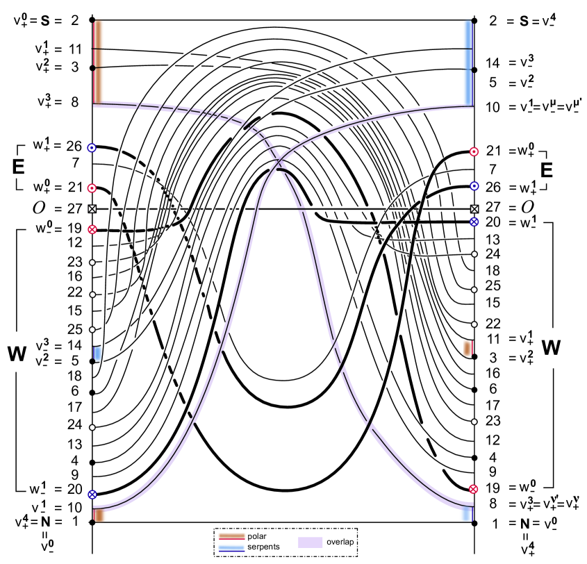
Figure 1.1: A sketch of the $27$ spatial profiles $v(x)$, for all equilibria in a solid Sturm octahedron $\mathcal{A}_{f}$. The equilibria $1,\ldots,27$ are ordered by $h_{0}^{f}$, $h_{1}^{f}$ along the left, right vertical axis $x=0,\,1$, respectively. Dots $\bullet$ indicate stable sink equilibria $1,\ldots,6$ with Morse index $i=0$. Circles $\circ$ indicate $8$ source equilibria $19,\ldots,26$ with unstable dimension $i=2$. The $i=3$ central equilibrium of the solid octahedron is $\mathcal{O}=27$. The remaining equilibria $7,\ldots,18$ indicate $i=1$ saddles. See also figs. 1.2 and 1.3. For the notations $v_{\pm}^{j},\ w_{\pm}^{\iota}$ see also fig. 1.5.

The dynamic consequences of the Sturm structure are enormous. In a series of papers, we have given a combinatorial description of Sturm global attractors $\mathcal{A}_{f}$; see [FiRo96, FiRo99, FiRo00]. Define the two labeling bijections $h^{f}_{0},h^{f}_{1}$: $\{1,\ldots,N\}\rightarrow\mathcal{E}_{f}$ of the equilibria such that

(1.5) $$h^{f}_{\iota}(1)<h^{f}_{\iota}(2)<\ldots<h^{f}_{\iota}(N)\qquad\text{at}\qquad x=\iota=0,1\,.$$

See figs. 1.1 and 5.1 for specific examples.

Our combinatorial description is based on the Sturm permutation $\sigma_{f}\in S_{N}$ which was introduced by Fusco and Rocha in [FuRo91] and is defined as

(1.6) $$\sigma_{f}\mathrel{\mathop{\mathchar 58\relax}}=(h^{f}_{0})^{-1}\circ h^{f}_{1}\,.$$

Using a shooting approach to the ODE boundary value problem (1.2), the Sturm permutations $\sigma_{f}\in S_{N}$ have been characterized as dissipative Morse meanders in [FiRo99]; see also (1.22)–(1.28) below for details. In [FiRo96] we have shown how to determine which equilibria $v$, $w$ possess a heteroclinic orbit connection (1.3), explicitly and purely combinatorially from $\sigma_{f}$. A remaining puzzle were different, and even nonconjugate, Sturm permutations which still give rise to $C^{0}$ orbit-equivalent Sturm attractors; see also [FiRo16, fig. 5.2]. We will address this puzzle in theorem 2.7 below.

Already at this elementary level, let us mention the four trivial equivalences generated by the two commuting involutions $x\mapsto 1-x$ and $u\mapsto-u$; see [FiRo16, definition 2.3]. Evidently, the first involution interchanges $h_{0}$ with $h_{1}$, and hence replaces the Sturm permutation $\sigma=h_{0}^{-1}\circ h_{1}$ by its inverse $\sigma^{-1}$. The second involution reverses the direction of the boundary orders $h_{0},h_{1}$. This replaces $\sigma$ by its conjugate $\kappa\sigma\kappa$ under the flip $\kappa(j)\mathrel{\mathop{\mathchar 58\relax}}=N+1-j$. Trivially, trivial equivalences give rise to trivially $C^{0}$ orbit-equivalent Sturm attractors. It is the remaining nontrivial equivalences, most of all, which theorem 2.7 aims at.

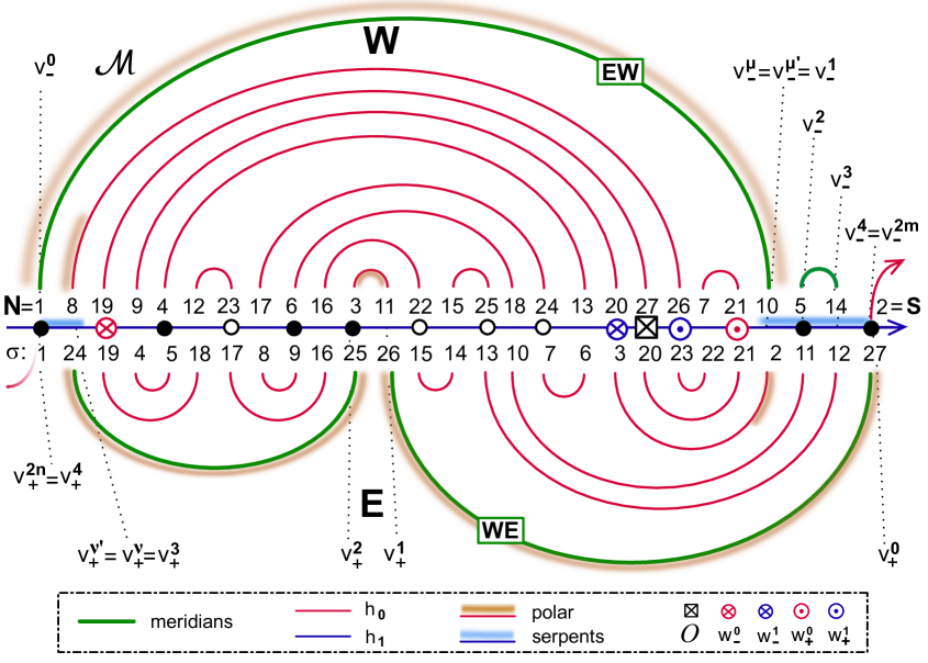
Figure 1.2: The Sturm meander $\mathcal{M}_{f}$ of the solid octahedron $\mathcal{A}_{f}$ of fig. 1.1. Equilibrium labels above the horizontal $h_{1}$-axis, and Sturm permutation $\sigma_{f}=(h_{0}^{f})^{-1}\circ h_{1}^{f}$ below. Note how the shooting curve $h_{0}^{f}$ and the horizontal axis $h_{1}^{f}$ follow the equilibrium labels according to their enumerations in fig. 1.2. Note consistency of all Morse numbers $i_{v}$ with Morse indices $i(v)$, for all equilibria $v$, according to fig. 1.1.

For an explicit example of a Sturm permutation $\sigma_{f}$ which defines a solid octahedral Sturm global attractor $\mathcal{A}_{f}$ see figs. 1.1 – 1.3 and [FiRo16, section 6]. Fig. 1.1 sketches the spatial profiles $v=v(x)$ for the $N=27$ equilibria $v\in\mathcal{E}_{f}$. The boundary label maps $h_{\iota}^{f}$ are, specifically,

(1.7) $$h_{0}\mathrel{\mathop{\mathchar 58\relax}}\,\,1 \text{10 20 9 4 13 24 17 6 18 5 14 25 15 22 16 23 12 19 27 21 7 26 8 3 11 2}\,;$$

$$h_{1}\mathrel{\mathop{\mathchar 58\relax}}\,\,1 \text{8 19 9 4 12 23 17 6 16 3 11 22 15 25 18 24 13 20 27 26 7 21 10 5 14 2}\,.$$

Fig. 1.2 depicts a stylized shooting meander $\mathcal{M}_{f}$ associated to the octahedral Sturm permutation $\sigma_{f}$ which results from the boundary labels $h_{\iota}^{f}$ of the equilibria $v\in\mathcal{E}_{f}$ at $x=\iota=0,1$, in ascending order. By (1.6) and (1.7),

(1.8) $$\sigma =\{1,\text{24, 19, 4, 5, 18, 17, 8, 9, 16, 25, 26, 15, 14,}$$

$$\phantom{=\{1,}\text{ 13, 10, 7, 6, 3, 20, 23, 22, 21, 2, 11, 12, 27}\}=$$

$$=\text{(2 24) (3 19) (6 18) (7 17) (10 16) (11 25) (12 26) (13 15) (21 23)}\,.$$

Indeed, the $(v,v_{x})$ phase plane of ODE (1.2) at $x=1$ features the horizontal $v$-axis with equilibrium order $h_{1}^{f}$, as a Neumann boundary condition. The meander curve $\mathcal{M}_{f}$ is the image, at $x=1$, which results, by shooting, from the Neumann initial conditions at $x=1$. Hence the intersections of $\mathcal{M}_{f}$ with the horizontal axis represent the equilibrium set $\mathcal{E}_{f}$. The ascending labeling $h_{0}^{f}$ of equilibria, at $x=0$, is the ordering of these intersections along $\mathcal{M}_{f}$. The ascending labeling $h_{1}^{f}$ of equilibria, at $x=1$, is the ordering of these same intersections along the horizontal axis.

In fact it is the Sturm property of (1.4) which implies the Morse-Smale property, for hyperbolic equilibria. Indeed unstable and stable manifolds $W^{u}(v)$, $W^{s}(w)$, which intersect precisely along heteroclinic orbits $v\leadsto w$, are automatically transverse: $W^{u}(v)\mathrel{\text{\vbox{ \halign{#\cr\smash{$-$}\crcr$\pitchfork$\crcr} }}}W^{s}(w)$. See [He85, An86]. In the Morse-Smale setting, Henry already observed, that a heteroclinic orbit $v\leadsto w$ is equivalent to $w$ belonging to the boundary $\partial W^{u}(v)$ of the unstable manifold $W^{u}(v_{-})$; see [He85].

More geometrically, global Sturm attractors $\mathcal{A}_{f}$ and $\mathcal{A}_{g}$ with the same Sturm permutation $\sigma_{f}=\sigma_{g}$ are $C^{0}$ orbit-equivalent [FiRo00]. Only for $C^{1}$-small perturbations, from $f$ to $g$, this global fact follows from $C^{0}$ structural stability of Morse-Smale systems; see e.g. [PaSm70] and [PaMe82].

For planar Sturm attractors $\mathcal{A}_{f}$, i.e. for equilibrium sets $\mathcal{E}_{f}$ with a maximal Morse index two [Br90, Jo89, Ro91], a slightly more geometric approach had been initiated in the planar Sturm trilogy [FiRo08, FiRo09, FiRo10]. It was clarified which planar graphs $\mathcal{H}$ do arise as connection graphs $\mathcal{H}=\mathcal{H}_{f}$ of planar Sturm attractors $\mathcal{A}_{f}$, and which ones do not. Meanwhile, a Schoenflies theorem has also been proved to hold for the closure $\overline{W}^{u}(v)\subseteq X$ of the unstable manifold $W^{u}$ of any hyperbolic equilibrium $v$; see [FiRo15]. In particular $\overline{W}^{u}(v)$ is the homeomorphic Euclidean embedding of a closed unit ball $\overline{B}^{i(v)}$ of dimension $i(v)$. In [FiRo14] this allowed us to reformulate the combinatorial results of [FiRo08, FiRo09, FiRo10], in a more geometric and topological language, as follows.

We consider finite regular CW-complexes

(1.9) $$\mathcal{C}=\bigcup\limits_{v\in\mathcal{E}}c_{v}\,,$$

i.e. finite disjoint unions of cell interiors $c_{v}$ with additional gluing properties. We think of the labels $v\in\mathcal{E}$ as barycenter elements of $c_{v}$. For CW-complexes we require the closures $\overline{c}_{v}$ in $\mathcal{C}$ to be the continuous images of closed unit balls $\overline{B}_{v}$ under characteristic maps. We call $\mathrm{dim}\,\overline{B}_{v}$ the dimension of the (open) cell $c_{v}$. For positive dimensions of $\overline{B}_{v}$ we require $c_{v}$ to be the homeomorphic images of the interiors $B_{v}$. For dimension zero we write $B_{v}\mathrel{\mathop{\mathchar 58\relax}}=\overline{B}_{v}$ so that any 0-cell $c_{v}=B_{v}$ is just a point. The m-skeleton $\mathcal{C}^{m}$ of $\mathcal{C}$ consists of all cells of dimension at most $m$. We require $\partial c_{v}\mathrel{\mathop{\mathchar 58\relax}}=\overline{c}_{v}\setminus c_{v}\subseteq\mathcal{C}^{m-1}$ for any $m$-cell $c_{v}$. Thus, the boundary $(m-1)$-sphere $S_{v}\mathrel{\mathop{\mathchar 58\relax}}=\partial B_{v}=\overline{B}_{v}\setminus B_{v}$ of any $m$-ball $B_{v}$, $m>0$, maps into the $(m-1)$-skeleton,

(1.10) $$\partial B_{v}\quad\longrightarrow\quad\partial c_{v}\subseteq\mathcal{C}^{m-1}\,,$$

for the $m$-cell $c_{v}$, by restriction of the continuous characteristic map. The map (1.10) is called the attaching (or gluing) map. For regular CW-complexes, in contrast, the characteristic maps $\overline{B}_{v}\rightarrow\overline{c}_{v}$ are required to be homeomorphisms, up to and including the attaching (or gluing) homeomorphism. We moreover require $\partial{c_{v}}$ to be a sub-complex of $\mathcal{C}^{m-1}$, then. See [FrPi90] for a background on this terminology.

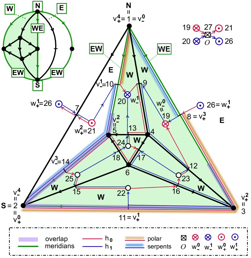
Figure 1.3: Sketch of the labeling bijections $(h_{0}^{f},h_{1}^{f})$ in the bipolar dynamic 3-cell complex of the solid octahedron $\mathcal{A}_{f}$ of fig. 1.1. The backwards face $1\,2\,3$ of the octahedron is exterior. Note the hemisphere decomposition $\mathbf{W}$, $\mathbf{E}$ by the two meridians $\mathbf{EW}$ and $\mathbf{WE}$ from pole $\mathbf{N}$ to pole $\mathbf{S}$. The paths $h_{\iota}^{f}$ with respect to equilibrium labels in the figure are listed in (1.7). See also (1.8) for the resulting Sturm permutation $\sigma=h_{0}^{-1}\circ h_{1}$, and fig. 1.2 for the resulting Sturm meander.

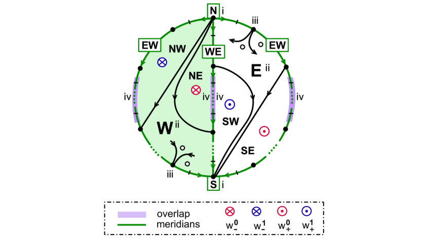
Figure 1.4: A 3-cell template. Shown is the $S^{2}$ boundary of the single 3-cell $c_{\mathcal{O}}$ with poles $\mathbf{N}$, $\mathbf{S}$, hemispheres $\mathbf{W}$ (green), $\mathbf{E}$ and separating meridians $\mathbf{EW}$, $\mathbf{WE}$ (green). The right and the left boundaries denote the same $\mathbf{EW}$ meridian and have to be identified. Dots $\bullet$ are sinks, and small circles $\circ$ are sources. Note the hemisphere decomposition (ii), the edge orientations (iii) at meridian boundaries, and the meridian overlaps (iv) of the $\mathbf{N}$-adjacent meridian faces $\otimes=w_{-}^{\iota}$ with their $\mathbf{S}$-adjacent counterparts $\odot=w_{+}^{\iota}$. For $w_{\pm}^{\iota}$ see also (1.29). For a specific octahedron example see fig. 1.3.

The disjoint dynamic decomposition

(1.11) $$\mathcal{A}_{f}=\bigcup\limits_{v\in\mathcal{E}_{f}}W^{u}(v)$$

of the global attractor $\mathcal{A}_{f}$ into unstable manifolds $W^{u}$ of equilibria $v$ is called the Thom-Smale complex or dynamic complex; see for example [Fr79, Bo88, BiZh92]. In our Sturm setting (1.1) with hyperbolic equilibria $v\in\mathcal{E}_{f}$, the Thom-Smale complex is a finite regular CW-complex. The open cells $c_{v}$ are the unstable manifolds $W^{u}(v)$ of the equilibria $v\in\mathcal{E}_{f}$. The proof is closely related to the Schoenflies result of [FiRo15]; see [FiRo14]. We can therefore define the Sturm complex $\mathcal{C}_{f}$ to be the regular Thom-Smale dynamic complex

(1.12) $$\mathcal{C}_{f}\mathrel{\mathop{\mathchar 58\relax}}=\bigcup_{v\in\mathcal{E}_{f}}\,W^{u}(v)$$

of the Sturm global attractor $\mathcal{A}_{f}$, provided all equilibria $v\in\mathcal{E}_{f}$ are hyperbolic. Again we call the equilibrium $v\in\mathcal{E}_{f}$ the barycenter of the cell $c_{v}=W^{u}(v)$.

A planar Sturm complex $\mathcal{C}_{f}$, for example, is the Thom-Smale complex of a planar Sturm global attractor $\mathcal{A}_{f}$ for which all equilibria $v\in\mathcal{E}_{f}$ have Morse indices $i(v)\leq 2$. See section 3 for a detailed discussion, based on our planar Sturm trilogy [FiRo08, FiRo09, FiRo10]. See fig. 1.3 for the Sturm complex of the solid octahedron attractor $\mathcal{A}_{f}$ defined by the Sturm permutation $\sigma_{f}$ of (1.8) and figs. 1.1, 1.2.

Our main objective, in the present trilogy of papers, is a geometric and combinatorial characterization of those global Sturm attractors, which are the closure

(1.13) $$\mathcal{A}_{f}=\text{clos }W^{u}(\mathcal{O})$$

of the unstable manifold $W^{u}$ of a single equilibrium $v=\mathcal{O}$ with Morse index $i(\mathcal{O})=3$. We call such an $\mathcal{A}_{f}$ a 3-ball Sturm attractor. Recall that we assume all equilibria $v\in\mathcal{E}_{f}$ to be hyperbolic: sinks have Morse index $i=0$, saddles have $i=1$, and sources $i=2$. This terminology also applies when viewed within the flow-invariant and attracting boundary 2-sphere

(1.14) $$\Sigma^{2}=\partial W^{u}(\mathcal{O})\mathrel{\mathop{\mathchar 58\relax}}=\left(\text{clos }W^{u}(\mathcal{O})\right)\smallsetminus W^{u}(\mathcal{O})\,.$$

Correspondingly we call the associated cells $c_{v}=W^{u}(v)$ of the dynamic cell complex, or of any regular cell complex, vertices, edges, and faces. The graph of vertices and edges, for example, defines the 1-skeleton $\mathcal{C}^{1}$ of the 3-ball cell complex $\mathcal{C}=\bigcup_{v}\,c_{v}$.

For a geometric characterization of 3-ball Sturm attractors $\mathcal{A}_{f}$ in (1.13), by their dynamic complexes (1.11), we now drop all Sturmian PDE interpretations. Instead we define 3-cell templates, abstractly, in the class of regular cell complexes and without any reference to PDE or dynamics terminology. See fig. 1.4 for an illustration.

Definition 1.1.

A finite disjoint union $\mathcal{C}=\bigcup_{v\in\mathcal{E}}c_{v}$ of cells $c_{v}$ is called a 3-cell template if $\mathcal{C}$ is a regular cell complex and the following four conditions all hold.

• $\mathcal{C}=\text{clos }c_{\mathcal{O}}=S^{2}\,\dot{\cup}\,c_{\mathcal{O}}$ is the closure of a single 3-cell $c_{\mathcal{O}}$.

• The 1-skeleton $\mathcal{C}^{1}$ of $\mathcal{C}$ possesses a bipolar orientation from a pole vertex $\mathbf{N}$ (North) to a pole vertex $\mathbf{S}$ (South), with two disjoint directed meridian paths $\mathbf{WE}$ and $\mathbf{EW}$ from $\mathbf{N}$ to $\mathbf{S}$. The circle of meridians decomposes the boundary sphere $S^{2}$ into remaining hemisphere components $\mathbf{W}$ (West) and $\mathbf{E}$ (East), both open in $S^{2}$.

• Edges are oriented towards the meridians, in $\mathbf{W}$, and away from the meridians, in $\mathbf{E}$, at end points on the meridians other than the poles $\mathbf{N}$, $\mathbf{S}$.

• Let $\mathbf{NE}$, $\mathbf{SW}$ denote the unique faces in $\mathbf{W}$, $\mathbf{E}$, respectively, which contain the first, last edge of the meridian $\mathbf{WE}$ in their boundary. Then the boundaries of $\mathbf{NE}$ and $\mathbf{SW}$ overlap in at least one shared edge of the meridian $\mathbf{WE}$.

  Similarly, let $\mathbf{NW}$, $\mathbf{SE}$ denote the unique faces in $\mathbf{W}$, $\mathbf{E}$, adjacent to the first, last edge of the other meridian $\mathbf{EW}$, respectively. Then their boundaries overlap in at least one shared edge of $\mathbf{EW}$.

We recall here that an edge orientation of the 1-skeleton $\mathcal{C}^{1}$ is called bipolar if it is without directed cycles, and with a single “source” vertex $\mathbf{N}$ and a single “sink” vertex $\mathbf{S}$ on the boundary of $\mathcal{C}$. Here “source” and “sink” are understood, not dynamically but, with respect to edge orientation. To avoid any confusion with dynamic $i=0$ sinks and $i=2$ sources, below, we call $\mathbf{N}$ and $\mathbf{S}$ the North and South pole, respectively.

With the above notation and definition we can now formulate the main result of the present paper.

Theorem 1.2.

Let $\mathcal{C}=\bigcup_{v\in\mathcal{E}}c_{v}$ be a finite disjoint union of cells. Then $\mathcal{C}=\mathcal{C}_{f}$ is the Thom-Smale dynamic cell complex of a 3-ball Sturm attractor $\mathcal{A}_{f}$ if, and only if, $\mathcal{C}$ is a 3-cell template. More precisely, there exists a cell-preserving homeomorphism

(1.15) $$\Phi\mathrel{\mathop{\mathchar 58\relax}}\qquad\mathcal{C}=\bigcup\limits_{v\in\mathcal{E}}c_{v}\quad\longrightarrow\quad\bigcup\limits_{v\in\mathcal{E}_{f}}W^{u}(v)=\mathcal{C}_{f}=\mathcal{A}_{f}$$

with $\Phi(c_{v})=W^{u}\left(\Phi(v)\right)$.

Here $\Phi$ also identifies the abstract labels $v\in\mathcal{E}$ of the cells $c_{v}$ with the generating equilibria $\Phi(v)\in\mathcal{E}_{f}$ of the unstable manifolds $W^{u}(v)$ of Morse index dimension $\dim c_{v}=i(v)$.

In [FiRo14] we have proved a precursor of theorem 1.2: any finite regular cell complex which is the closure of a single 3-cell is, in fact, the dynamic complex of a suitable Sturm 3-ball. This requires condition (i) of definition 1.1, only. The full geometric characterization of Sturm 3-balls as 3-cell templates, in theorem 1.2, is much more detailed, of course. It turns out that any finite regular 2-sphere complex possesses a bipolar orientation, with edge adjacent poles, and a hemisphere decomposition, with a single Western face, which defines a 3-cell template. Therefore theorem 1.2 refines [FiRo14].

In section 2 we translate the geographic language of definition 1.1, for 3-cell templates, into the broader concept of signed hemisphere decompositions. At the heart of this is a convenient notational variant of the zero number $z$. We write

(1.16) $$z(\varphi)=j_{\pm}$$

to indicate $j$ strict sign changes of $\varphi$, by $j$, and $\pm\varphi(0)>0$, by the index $\pm$. For example $z(\pm\varphi_{j})=j_{\pm}$, for the $j$-th Sturm-Liouville eigenfunction $\varphi_{j}$. By the Schoenflies result [FiRo15] and [FiRo16, proposition 3.1] this provides a disjoint signed hemisphere decomposition

(1.17) $$\partial W^{u}(v)=\bigcup\limits_{0\leq j<i(v)}\Sigma_{\pm}^{j}(v)$$

of the boundary sphere $\Sigma^{i(v)-1}=\partial W^{u}(v)$ of any unstable manifold, such that

(1.18) $$\Sigma_{\pm}^{j}(v)\mathrel{\mathop{\mathchar 58\relax}}=\bigcup_{\begin{subarray}{c}v\leadsto w\\ z(w-v)=j_{\pm}\end{subarray}}W^{u}(w)\,.$$

For the fast unstable manifolds $W^{k}$ of $v$ with dimensions $1\leq k\leq i(v)$, we obtain analogously

(1.19) $$\partial W^{k}(v)=\bigcup\limits_{0\leq j<k}\Sigma_{\pm}^{j}(v)\,.$$

See (2.8)–(2.15) for details. With the abbreviation $\Sigma_{\pm}^{j}$:= $\Sigma_{\pm}^{j}(\mathcal{O})$, the translation table between the signed hemispheres decomposition (1.17), (1.18) of $\partial W^{u}(\mathcal{O})=\mathcal{A}_{f}\smallsetminus W^{u}(\mathcal{O})$, for the Sturm 3-ball $\mathcal{A}_{f}$ in theorem 1.2, and the geographic 3-cell template $\mathcal{C}$ of definition 1.1, is as follows:

(1.20) $$(\Sigma_{-}^{0},\Sigma_{+}^{0}) \mapsto\quad(\mathbf{N},\mathbf{S})$$

$$(\Sigma_{-}^{1},\Sigma_{+}^{1}) \mapsto\quad(\mathbf{EW},\mathbf{WE})$$

$$(\Sigma_{-}^{2},\Sigma_{+}^{2}) \mapsto\quad(\mathbf{W},\mathbf{E})\,.$$

In theorem 2.6 below we refine theorem 1.2, such that the homeomorphism $\Phi$ respects a signed hemisphere decomposition, not only for $\partial W^{u}(\mathcal{O})$ but, for the sphere boundary $\partial W^{u}(v)$ of any unstable manifold in $\mathcal{A}_{f}$. In theorem 2.7 we will show how the Sturm permutation $\sigma_{f}$, and therefore the Sturm global attractor $\mathcal{A}_{f}$ itself (up to $C^{0}$ orbit equivalence), is determined uniquely by the signed hemisphere decompositions (1.17), (1.18).

As an elementary example, in section 3, we review and adapt our results from the planar trilogy [FiRo08, FiRo09, FiRo10] to the present setting of signed hemispheres. Our focus is on the equivalence of boundary bipolar orientations with the above language of signed hemisphere decompositions and fast unstable manifolds. In particular we recall, and justify, the face transition rules of [FiRo16, definition 2.2] for ZS-pairs $(h_{0},h_{1})$ in bipolar planar cell complexes, in corollary 3.2, using the language of signed hemisphere complexes.

In [FiRo16, theorem 5.2] of part 1 we have associated a certain Sturm global attractor $\mathcal{A}_{f}$ to any abstractly given 3-cell template $\mathcal{C}$. In fact we have constructed abstract paths $h_{\iota}$ in $\mathcal{C}$, for $\iota=0,1$, by recipe or decree ex cathedra, such that the abstract permutation

(1.21) $$\sigma\mathrel{\mathop{\mathchar 58\relax}}=h_{0}^{-1}\circ h_{1}$$

was a dissipative Morse meander and hence, by [FiRo96], a Sturm permutation $\sigma=\sigma_{f}$ for some concrete nonlinearity $f$.

Let us now recall this terminology in some detail. Abstractly, a meander is an oriented planar $C^{1}$ Jordan curve $\mathcal{M}$ which crosses a positively oriented horizontal axis at finitely many points. The curve $\mathcal{M}$ is assumed to run from Southwest to Northeast, asymptotically, and all $N$ crossings are assumed to be transverse; see [Ar88, ArVi89]. Note $N$ is odd. Enumerating the $N$ crossing points $v\in\mathcal{E}$ along the meander $\mathcal{M}$ and along the horizontal axis, respectively, we obtain two labeling bijections

(1.22) $$h_{0},h_{1}\mathrel{\mathop{\mathchar 58\relax}}\quad\{1,\ldots,N\}\rightarrow\mathcal{E}\,.$$

Define the meander permutation $\sigma\in S_{N}$ as

(1.23) $$\sigma\mathrel{\mathop{\mathchar 58\relax}}=h_{0}^{-1}\circ h_{1}.$$

We call the meander $\mathcal{M}$ dissipative if

(1.24) $$\sigma(1)=1,\quad\sigma(N)=N$$

are fixed under $\sigma$. We define Morse numbers $i_{v}$ for the intersections $v\in\mathcal{E}$ of the meander $\mathcal{M}$ with the horizontal $h_{1}$-axis, recursively, by

(1.25) $$i_{h_{0}(1)} \mathrel{\mathop{\mathchar 58\relax}}=\quad i_{h_{0}(N)}\mathrel{\mathop{\mathchar 58\relax}}=\quad 0\,,$$

$$i_{h_{0}(j+1)} \mathrel{\mathop{\mathchar 58\relax}}=\quad i_{h_{0}(j)}+(-1)^{j+1}\text{sign}(\sigma^{-1}(j+1)-\sigma^{-1}(j))\,.$$

Equivalently, by recursion along $h_{1}$:

(1.26) $$i_{h_{1}(1)} \mathrel{\mathop{\mathchar 58\relax}}=\quad i_{h_{1}(N)}\mathrel{\mathop{\mathchar 58\relax}}=\quad 0\,,$$

$$i_{h_{1}(j+1)} \mathrel{\mathop{\mathchar 58\relax}}=\quad i_{h_{1}(j)}+(-1)^{j+1}\text{sign}(\sigma(j+1)-\sigma(j))\,.$$

Note how the enumeration of intersections $v\in\mathcal{E}$ by $h_{\iota}$: $\{1,\ldots,N\}\rightarrow\mathcal{E}$ depends on $h_{\iota}$, of course, but the Morse numbers $i_{v}$ only depend on the Sturm permutation $\sigma$ which defines the meander $\mathcal{M}$.

We call the meander $\mathcal{M}$ Morse, if

(1.27) $$i_{v}\geq 0\,,$$

for all $v\in\mathcal{M}$.

We call $\mathcal{M}$ Sturm meander, if $\mathcal{M}$ is a dissipative Morse meander; see [FiRo96]. Conversely, given any permutation $\sigma\in S_{N}$, we can define an associated curve $\mathcal{M}$ of arches over the horizontal axis which switches sides at the intersections $\mathcal{E}=\{1,\ldots,N\}$ on the axis, in the order of $\sigma$. This fixes the labeling $h_{1}=\mathrm{id}$ and $h_{0}=\sigma^{-1}$. A Sturm permutation $\sigma$ is a permutation such that the associated curve $\mathcal{M}$ is a Sturm meander. The main paradigm of [FiRo96] is the equivalence of Sturm meanders $\mathcal{M}$ with shooting curves of the Neumann ODE problem (1.2). In fact, the Neumann shooting curve is a Sturm meander, for any dissipative nonlinearity $f$ with hyperbolic equilibria. Conversely, for any permutation $\sigma$ of a Sturm meander $\mathcal{M}$ there exist dissipative $f$ with hyperbolic equilibria such that $\sigma=\sigma_{f}$ is the Sturm permutation of $f$. In particular, the intersections $v$ of the meander $\mathcal{M}$ with the horizontal $v$-axis are the boundary values of the equilibria $v\in\mathcal{E}_{f}$ at $x=1$, and the Morse number

(1.28) $$i_{v}=i(v)$$

is the Morse index of $v$. For that reason we have used closely related notation to describe either case.

In particular, (1.28) extends the terminology of sinks $i_{v}=0$, saddles $i_{v}=1$, and sources $i_{v}=2$ to abstract Sturm meanders. We insist, however, that our above definition (1.22)–(1.27) is completely abstract and independent of this ODE/PDE interpretation.

For example, consider the case $i_{\mathcal{O}}=3$ of a single intersection $v=\mathcal{O}$ with Morse number $3$. Suppose $i_{v}\leq 2$ for all other Morse numbers. Then (1.25) implies $i=2$ for the two $h_{0}$-neighbors $h_{0}(h_{0}^{-1}(\mathcal{O})\pm 1)$ of $\mathcal{O}$ along the meander $\mathcal{M}$. In other words, these neighbors are both sources. The same statement holds true for the two $h_{1}$-neighbors $h_{1}(h_{1}^{-1}(\mathcal{O})\pm 1)$ of $\mathcal{O}$ along the horizontal axis. To fix notation, we denote these $h_{\iota}$-neighbors by

(1.29) $$w_{\pm}^{\iota}\mathrel{\mathop{\mathchar 58\relax}}=h_{\iota}(h_{\iota}^{-1}(\mathcal{O})\pm 1)\,,$$

for $\iota=0,1$. The $h_{\iota}$-extreme sources are the first and last source intersections $v$ of the meander $\mathcal{M}$ with the horizontal axis, in the order of $h_{\iota}$.

Reminiscent of cell template terminology, we call the extreme sinks $\mathbf{N}=h_{0}(1)=h_{1}(1)$ and $\mathbf{S}=h_{0}(N)=h_{1}(N)$ the (North and South) poles of the Sturm meander $\mathcal{M}$. A polar $h_{\iota}$-serpent, for $\iota=0,1$, is a set of $v=h_{\iota}(m)\in\mathcal{E}$ for a maximal interval of integers $m$ which contains a pole, $\mathbf{N}$ or $\mathbf{S}$, such that

(1.30) $$i_{h_{\iota}(m)}\in\{0,1\}$$

for all $m$. To visualize the serpent we often include the meander or axis path joining $v$ in the serpent. See figs. 1.2 and 1.5 for examples. We call $\mathbf{N}$-polar serpents and $\mathbf{S}$-polar serpents anti-polar to each other. An overlap of anti-polar serpents simply indicates a nonempty intersection. For later reference, we call a polar $h_{\iota}$-serpent full if it extends all the way to the saddle which is $h_{1-\iota}$-adjacent to the opposite pole. Full $h_{\iota}$-serpents always overlap with their anti-polar $h_{1-\iota}$-serpent, of course, at least at that saddle.

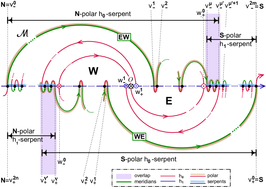
Figure 1.5: A 3-meander template. Note the $\mathbf{N}$-polar $h_{1}$-serpent $\mathbf{N}=v_{+}^{2n}\ldots v_{+}^{\nu}$ terminated at $v_{+}^{\nu}$ by the source $w_{-}^{0}$ which is, both, $h_{1}$-extreme minimal and the lower $h_{0}$-neighbor of $\mathcal{O}$. This serpent overlaps the anti-polar, i.e. $\mathbf{S}$-polar, $h_{0}$-serpent $v_{+}^{\nu^{\prime}}\ldots v_{+}^{\nu}\ldots v_{+}^{0}=\mathbf{S}$, from $v_{+}^{\nu^{\prime}}$ to $v_{+}^{\nu}$. Similarly, the $\mathbf{N}$-polar $h_{0}$-serpent $\mathbf{N}=v_{-}^{0}\ldots v_{-}^{\mu^{\prime}}$ overlaps the anti-polar, i.e. $\mathbf{S}$-polar, $h_{1}$-serpent $v_{-}^{\mu}\ldots v_{-}^{\mu^{\prime}}\ldots v_{-}^{2n}=\mathbf{S}$, from $v_{-}^{\mu}$ to $v_{-}^{\mu^{\prime}}$. The $h_{1}$-neighbors $w_{\pm}^{1}$ of $\mathcal{O}$ are the $h_{0}$-extreme sources, by the two polar $h_{0}$-serpents. Similarly, the $h_{0}$-neighbors $w_{\pm}^{0}$ of $\mathcal{O}$ define the $h_{1}$-extreme sources. Compare also the octahedral example of fig. 1.2.

Definition 1.3.

An abstract Sturm meander $\mathcal{M}$ with axis intersections $v\in\mathcal{E}$ is called a 3-meander template if the following four conditions hold, for $\iota=0,1$.

• $\mathcal{M}$ possesses a single axis intersection $v=\mathcal{O}$ with Morse number $i_{\mathcal{O}}=3$, and no other Morse number exceeds $2$.

• Polar $h_{\iota}$-serpents overlap with their anti-polar $h_{1-\iota}$-serpents in at least one shared vertex.

• The intersection $v=\mathcal{O}$ is located between the two intersection points, in the order of $h_{1-\iota}$, of the polar arc of any polar $h_{\iota}$-serpent.

• The $h_{\iota}$-neighbors $w^{\iota}_{\pm}$ of $v=\mathcal{O}$ are the $i=2$ sources which terminate the polar $h_{1-\iota}$-serpents.

See fig. 1.5 for an illustration of 3-meander templates. Property (iv), for example, asserts that the $h_{\iota}$-neighbor sources $w_{\pm}^{\iota}$ of $\mathcal{O}$ are the $h_{1-\iota}$-extreme sources, for $\iota=0,1$. For the Sturm boundary orders $h^{f}_{\iota}$ this is a useful exercise in polar serpents; see [FiRo16, lemma 4.3(iii)].

In [FiRo16, theorem 5.2] we have established the passage

(1.31) $$\text{3-cell template}\quad\Longrightarrow\quad\text{3-meander template}\,,$$

based on the above construction. The 3-meander template $\mathcal{M}$ and its Sturm permutation $\sigma=h_{0}^{-1}h_{1}$, in turn, define a Sturm nonlinearity $f$ such that $\sigma_{f}=\sigma$. Let $\mathcal{A}_{f}$ denote the Sturm global attractor of $f$.

In theorem 5.1 below, we claim that $\mathcal{A}_{f}$ is in fact a Sturm 3-ball. We prepare the proof, in section 4, by a formal scoop of noses and signed hemispheres, which does not affect heteroclinic connectivity in the closure of the opposite hemisphere; see (4.4) and definition 4.2.

We prove the refined version, theorem 2.6, of theorem 1.2, and uniqueness theorem 2.7 on the Sturm permutations of prescribed Sturm 3-cell templates, in the final section 7. This is based on the crucial identity

(1.32) $$h_{\iota}^{f}=h_{\iota}$$

between the labeling orders $h_{\iota}^{f}$: $\{1,\ldots,N\}\rightarrow\mathcal{E}_{f}$ of equilibria $v\in\mathcal{E}_{f}$, according to the order of their boundary values $v(x)$ at $x=\iota=0,1$, and the SZS labeling paths $h_{\iota}$ in the abstract Sturm complex $\mathcal{C}=\mathcal{C}_{f}$ of the cells $c_{v}=W^{u}(v)$, for all $v\in\mathcal{E}=\mathcal{E}_{f}$. More precisely we will prove (1.32) for the scoops $\check{h}_{\iota}$ and the paths $h_{\iota}^{\pm}$ defined by the abstract planar signed hemisphere complexes; see lemma 6.1. In particular, the signed hemisphere complexes $\mathcal{C}_{f}^{s}$ of Sturm 3-ball attractors are in one-to-one correspondence with 3-template cell complexes, which are signed complexes $\mathcal{C}^{s}$, via the translation table (1.20). This shows that any prescribed 3-cell template $\mathcal{C}$ can be realized as the signed hemisphere complex $\mathcal{C}_{f}^{s}$ of a Sturm 3-ball attractor $\mathcal{A}_{f}$. It also shows how $\mathcal{C}$ determines $\sigma=\sigma_{f}$ uniquely; see theorem 2.7. Moreover it closes the cycle of implications

(1.33)

for Sturm 3-balls.

Acknowledgments. With great pleasure we express our profound gratitude to Waldyr M. Oliva, whose deep geometric insights and friendly challenges remain a visible inspiration to us since so many years. Extended mutually delightful hospitality by the authors is mutually acknowledged. Suggestions concerning the Thom-Smale complex were generously provided by Jean-Michel Bismut. Gustavo Granja has generously shared his deeply topological view point, precise references included. Anna Karnauhova has contributed all illustrations with great patience, ambition, and her inimitable artistic touch. Typesetting was expertly accomplished by Ulrike Geiger. This work was partially supported by DFG/Germany through SFB 647 project C8 and by FCT/Portugal through project UID/MAT/04459/2013.

2 Signed hemispheres

The basic tool in the proof of our main theorem 1.2, and its refinements, is a detailed analysis of the signed zero number

(2.1) $$z(\varphi)=j_{\pm}\,,$$

which denotes $z(\varphi)=j$ and $\pm\varphi(0)>0$; see (1.16). In definition 2.1 below, this is used to define configurations of Sturm equilibria $v\in\mathcal{E}_{f}$ which we call signed hemisphere templates. We recall how to derive the relevant information from Sturm permutations $\sigma_{f}$, directly and explicitly. For independent readability later on, we also discuss Morse indices $i(v)$ and (signed) connection graphs $\mathcal{H}_{f}^{(s)}$, briefly. Proposition 2.2 recalls, from [FiRo16], how signed zero numbers relate to the hemisphere decomposition by boundaries $\partial W^{j}$ of fast unstable manifolds $W^{j}$. In proposition 2.3 we return to the planar and 3-ball cases, to summarize how the boundary label paths $h_{\iota}^{f}$ of the equilibrium orders (1.5) at $x=\iota=0,1$ traverse edges $W^{u}(v)$ of $i(v)=1$ saddles, faces $W^{u}(v)$ of $i(v)=2$ sources, and the 3-ball $W^{u}(\mathcal{O})$ of $i(\mathcal{O})=3$, in the Thom-Smale dynamic complex $\mathcal{C}_{f}$ of a Sturm 3-ball $\mathcal{A}_{f}$. We compare this description with the formal definition of formal ZS-pairs and SZS-pairs $(h_{0},h_{1})$ in 3-ball templates. Compare [FiRo16, definitions 2.2, 5.1] and definitions 2.4, 2.5 below. Noting the equivalence of proposition 2.3 and definition 2.5, in section 7, will prove theorem 2.6 which refines our main theorem 1.2: we establish the existence of a Sturm 3-ball attractor $\mathcal{A}_{f}$ such that the signed Thom-Smale complex $\mathcal{C}_{f}^{s}$ of $\mathcal{A}_{f}$ coincides with any prescribed 3-cell template (1.20). The equivalence is by a cell-preserving signed homeomorphism $\Phi^{s}$, as in (1.15), which also preserves the additional sign structure. We conclude, in theorem 2.7, by stating uniqueness of the Sturm permutation $\sigma_{f}$, as defined by the prescribed 3-cell template.

Let $\mathcal{A}_{f}$ be any Sturm global attractor. Recall how $\mathcal{A}_{f}$ comes with boundary label paths $h_{\iota}^{f}$, the Sturm permutation $\sigma_{f}=(h_{0}^{f})^{-1}\circ h_{1}^{f}$ and its meander $\mathcal{M}_{f}$, the set $\mathcal{E}_{f}$ of (hyperbolic) equilibria, and heteroclinic orbits $w\leadsto v$ between certain equilibria $w,v\in\mathcal{E}_{f}$. We write

(2.2) $$v\,\leadsto_{\pm}\,w\,,$$

if $v\leadsto w$ and $\pm(w-v)>0$ at $x=0$, respectively. The directed connection graph $\mathcal{H}_{f}$ consists of the equilibrium vertices $\mathcal{E}_{f}$ and directed edges $w\leadsto v$, indicating heteroclinic orbits between equilibria of adjacent Morse indices $i(w)=i(v)+1$. Due to a cascading principle, general heteroclinic orbits $w\leadsto v$, between not necessarily adjacent Morse levels $i$, are equivalently represented by di-paths in $\mathcal{H}_{f}$; see [BrFi89, FiRo96] and the summary in [FiRo16]. The signed connection graph $\mathcal{H}_{f}^{s}$, analogously, features signed directed edges $\leadsto_{\pm}$, instead.

Fix any unstable equilibrium $v\in\mathcal{E}_{f}$, with Morse index $i(v)=\dim W^{u}(v)>0$. We decompose the heteroclinic targets $v\leadsto w$ according to their signed zero number (2.1) as

(2.3) $$\mathcal{E}_{\pm}^{j}(v) \mathrel{\mathop{\mathchar 58\relax}}=\{w\in\mathcal{E}_{f}\,|\,v\leadsto_{\pm}w\,,\,z(w-v)=j\}$$

$$\phantom{\mathrel{\mathop{\mathchar 58\relax}}}=\{w\in\mathcal{E}_{f}\,|\,v\leadsto w\,,\,z(w-v)=j_{\pm}\}\,.$$

Here $0\leq j<i(v)$, because $j=z(u-v)<i(v)$ for all $u\in\text{clos }W^{u}(v)\smallsetminus\{v\}$; see [BrFi86].

Definition 2.1.

We call the partitions $\mathcal{E}_{\pm}^{j}(v)$, $0\leq j<i(v)$, of the equilibria $w\in\partial W^{u}(v)$, the signed hemisphere template of the Sturm attractor $\mathcal{A}_{f}$.

In the special case of a Sturm 3-ball $\mathcal{A}_{f}$ we call these partitions the signed 2-hemisphere template.

The relevant Morse and Sturm data $i(v)$ and $z(w-v)$ can easily be derived, explicitly, from the labeling paths $h_{\iota}=h_{\iota}^{f}\in S_{N}$ in (1.5) and the Sturm permutation $\sigma=\sigma_{f}=(h_{0}^{f})^{-1}\circ h_{1}^{f}$, as follows. Recursively, the Morse numbers $i_{v}$, $v\in\mathcal{E}_{f}$ have been defined in (1.21). Then [FuRo91] have shown that

(2.4) $$i(v)=i_{v}$$

for all $v\in\mathcal{E}_{f}$. Similarly, define the zero numbers $z_{v_{1}v_{2}}$ for $v_{1},v_{2}\in\mathcal{E}_{f}$, recursively, as

(2.5) $$z_{vv} \mathrel{\mathop{\mathchar 58\relax}}=i(v)\,,$$

$$z_{h_{0}(j+1)h_{0}(k)} \mathrel{\mathop{\mathchar 58\relax}}=z_{h_{0}(j)h_{0}(k)}+\tfrac{1}{2}(-1)^{j+1}\cdot$$

$$\phantom{\mathrel{\mathop{\mathchar 58\relax}}}\cdot\left[\text{sign}\left(\sigma^{-1}(j+1)-\sigma^{-1}(k)\right)-\text{sign}\left(\sigma^{-1}(j)-\sigma^{-1}(k)\right)\right]\,.$$

Then [Ro91, FiRo96] have shown that

(2.6) $$z(w-v)=z_{wv}\,.$$

for equilibria $w\neq v$. The signed version of (2.6) follows easily from $\text{sign}(h_{0}^{-1}(w)-h_{0}^{-1}(v))$.

Definition 2.1 in fact provides partitions of the equilibria $w\in\partial W^{u}(v)$, with the exception of those $w$ which are never the target of any heteroclinic orbit $v\leadsto w$ from some equilibrium $v$ with higher Morse index $i(v)>i(w)$. In the case of signed 2-hemisphere templates, this only excludes the 3-ball equilibrium $w=\mathcal{O}$ with $i(w)=3$. To see this we invoke the Morse-Smale property again; see section 1. Indeed all equilibria $w\in\partial W^{u}(v)$ are then targets of heteroclinic orbits $v\leadsto w$. This shows the equivalence of the connection graph $\mathcal{H}_{f}$ with the incidence relations,

(2.7) $$v\leadsto w\quad\Longleftrightarrow\quad c_{w}\subseteq\partial c_{v}\,.$$

in the Sturm complex of cells $c_{w}\subseteq\partial c_{v}$. For example, any equilibrium $w\neq\mathcal{O}$ satisfies $w\in\partial W^{u}(\mathcal{O})$, and is therefore the target of a heteroclinic orbit $\mathcal{O}\leadsto w$.

Our definition 2.1 of signed hemisphere templates differs slightly from the corresponding notion in [FiRo16, definition 1.1]. To clarify this point we have to recall first how the Schoenflies result [FiRo15] provides a disjoint hemisphere decomposition

(2.8) $$\partial W^{u}(v)=\bigcup\limits_{0\leq j<i(v)}\Sigma_{\pm}^{j}$$

of the topological boundary $\partial W^{u}$:= $\text{clos }W^{u}(v)\smallsetminus W^{u}(v)$ of the unstable manifold $W^{u}(v)$, for any hyperbolic equilibrium $v$. The construction of the disjoint hemispheres $\Sigma_{\pm}^{j}=\Sigma_{\pm}^{j}(v)$ can be summarized as follows. For $1\leq j\leq i(v)$, let $W^{j}$ denote the $j$-dimensional fast unstable manifold of $v$. The tangent space to $W^{j}$ at $v$ is spanned by the eigenfunctions $\varphi_{0},\ldots,\varphi_{j-1}$ of the linearization of (1.2) at $v$, for the first $j$ eigenvalues $\lambda_{0}>\ldots>\lambda_{j-1}>0$. Consider any orbit $u(t,\cdot)\in W^{j+1}\smallsetminus W^{j}$, $t\in\mathbb{R}$. Then

(2.9) $$\lim_{t\rightarrow-\infty}\left(u\left(t,\cdot\right)-v\right)\,/\,|u\left(t,\cdot\right)-v|=\pm\varphi_{j}\,;$$

by normalization of $\varphi_{j}$ in the appropriate norm of the phase space $X\hookrightarrow C^{1}$. Here and below we fix signs such that $\varphi_{j}(0)>0$. In particular, the signed zero number $z$ of (1.4) satisfies

(2.10) $$\lim_{t\rightarrow-\infty}z\left(u\left(t,\cdot\right)-v\right)=z(\pm\varphi_{j})=j_{\pm}\,.$$

See [BrFi86] for further details on the construction of $W^{j}$.

The signed hemispheres $\Sigma_{\pm}^{j}$ are defined, recursively, by the disjoint unions

(2.11) $$\Sigma^{j}\mathrel{\mathop{\mathchar 58\relax}}=\partial W^{j+1}=\Sigma_{-}^{j}\,\cup\,\Sigma_{+}^{j}\,\cup\,\Sigma^{j-1}\,,$$

for $0\leq j<i(v)$, with the convention $\Sigma^{-1}$:= $\emptyset$. The hemisphere closures

(2.12) $$\text{clos }\Sigma_{\pm}^{j}=\Sigma_{\pm}^{j}\,\dot{\cup}\,\Sigma^{j-1}$$

can be obtained as $\omega$-limit sets of protocap hemispheres which are $C^{1}$-small, nearly parallel, perturbations of $\text{clos }W^{j}$ in $\text{clos }W^{j+1}$, in the eigendirections $\pm\varphi_{j}$, respectively. In particular (2.9), (2.10) hold in the interior of the protocaps, and for any heteroclinic orbit $v\leadsto w\in\Sigma_{\pm}^{j}$. See [FiRo15] for complete details.

The following proposition was proved in [FiRo16, proposition 3.1], again with the abbreviations $\Sigma_{\pm}^{j}=\Sigma_{\pm}^{j}(v)$.

Proposition 2.2.

With the above notation the following statements hold true for equilibria $v,w,w_{1},w_{2},$ and all $0\leq j<i(v)$:

(i) $$w\in\Sigma^{j}\quad \Longrightarrow\quad i(w)\leq j\;$$

(ii) $$w\in\Sigma^{j}\quad \Longrightarrow\quad z(w-v)\leq j\;$$

(iii) $$w\in\Sigma_{\pm}^{j}\quad \Longrightarrow\quad z(w-v)=j_{\pm}\;$$

(iv) $$w_{1},w_{2}\in\text{clos }\Sigma_{+}^{j}\text{ or }w_{1},w_{2}\in\text{clos }\Sigma_{-}^{j}\quad \Longrightarrow\quad z(w_{1}-w_{2})\leq j-1\,.$$

In [FiRo16, definition 1.1] the sets $\mathcal{E}_{\pm}^{j}(v)$ of the signed hemisphere templates (2.3) had been defined as

(2.13) $$\tilde{\mathcal{E}}_{\pm}^{j}(v)\mathrel{\mathop{\mathchar 58\relax}}=\mathcal{E}_{f}\cap\Sigma_{\pm}^{j}(v)\,,$$

instead. By proposition 2.2(iii), the sets $\mathcal{E}_{\pm}^{j}(v)$ and $\tilde{\mathcal{E}}_{\pm}^{j}(v)$ coincide, for each $j$.

Conversely, we can describe the signed hemispheres $\Sigma_{\pm}^{j}(v)$ directly, via the signed hemisphere template (2.3) of equilibrium sets $\mathcal{E}_{\pm}^{j}(v)$. Indeed (1.18) now reads

(2.14) $$\Sigma_{\pm}^{j}(v)=\bigcup\limits_{w\in\mathcal{E}_{\pm}^{j}(v)}W^{u}(w)\,.$$

This allows us to define a signed Sturm complex $\mathcal{C}_{f}^{s}$, as a refinement of the Sturm complex $\mathcal{C}_{f}$ with (regular) Thom-Smale cells $W^{u}(v)$, $v\in\mathcal{E}_{f}$. We simply keep track, in $\mathcal{C}_{f}^{s}$, which cells $W^{u}(w)$ of $\mathcal{C}_{f}$ belong to which hemisphere $\Sigma_{\pm}^{j}(v)$ in the signed hemisphere decomposition of $\mathcal{C}_{f}$.

We now focus on the case of a Sturm 3-ball $\mathcal{A}_{f}$. Our next proposition describes, in terms of the dynamic cell decompositions of $\mathcal{A}_{f}$ by the Thom-Smale cells $c_{v}\in W^{u}(v)$, how the labeling bijections $h_{\iota}^{f}$, $\iota=0,1$, traverse each cell. Let $0<n$:= $i(v)\leq 3$ be the Morse index of $v$. For fixed $n$, consider sequences $\mathbf{s}=s_{0}\ldots s_{n-1}$ of $n$ symbols $s_{i}\in\left\{\pm\right\}$. In fact, let us restrict to the four cases of constant and alternating sequences of signs $s_{i}$. For any such prescribed sequence $\mathbf{s}=s_{0}\ldots s_{n-1}$ let $w=w(\mathbf{s})\in\Sigma_{s_{n-1}}^{n-1}(v)$ denote the unique equilibrium such that $v\leadsto w$ starts a heteroclinic cascade

(2.15) $$v\leadsto v_{n-1}\leadsto\ldots\leadsto v_{0}$$

with $w=v_{n-1}$ and $v_{i}\in\Sigma_{s_{i}}^{i}(v)$ of descending Morse indices $i(v_{i})=i=n-1,\ldots,0$. Equivalently, by (2.7), we may express the same definition on the level of Thom-Smale cells as

(2.16) $$c_{v_{i}}\subseteq\partial c_{v_{i+1}}\cap\Sigma_{s_{i}}^{i}(v)\,,$$

with $v=v_{n},\ w=w_{n-1}$, and $v_{i}\in\Sigma_{s_{i}}^{i}(v)$ of ascending Morse indices $i(v_{i})=i=0,\ldots,n-1$.

Again, we do not claim existence of $w(\mathbf{s})$ except in the four cases of constant and alternating signs $s_{i}$. Uniqueness of $w(\mathbf{s})$, for given symbol sequence $\mathbf{s}$, can be proved by induction on $n$. For some $v$, however, certain equilibria $w(\mathbf{s})$ with different symbol sequences may happen to coincide.

Proposition 2.3.

Fix $0<n$:= $i(v)\leq 3$, $\iota=0,1$, and assume $v\in\mathcal{E}_{f}$ is not already directly preceded, or directly followed, by an equilibrium of higher Morse index than $n=i(v)$, along the labeling bijection $h_{\iota}^{f}\mathrel{\mathop{\mathchar 58\relax}}\{1,\ldots,N\}\rightarrow\mathcal{E}_{f}$. Then the unclaimed parts of $h_{\iota}^{f}$ through $v$ follow the template table

	$h_{0}^{f}$	$h_{1}^{f}$
$n=i(v)=1$	$\ldots w(-)\,v\,w(+)\ldots$	$\ldots w(-)\,v\,w(+)\ldots$
$n=i(v)=2$	$\ldots w(+-)\,v\,w(-+)\ldots$	$\ldots w(++)\,v\,w(--)\ldots$
$n=i(v)=3$	$\ldots w(-+-)\,v\,w(+-+)\ldots$	$\ldots w(---)\,v\,w(+++)\ldots$

Proof..

By adjacency (1.25), (1.26) of Morse indices for $h_{\iota}$-adjacent equilibria, we only have to consider the case $i(w)=n-1$, $i(v)=n$ for the $w$-entries in the table. In particular, the unique heteroclinic orbits $u(t)$:= $v\leadsto w$ imply $z(w-v)=(n-1)_{s_{n-1}}$ with

(2.17) $$s_{n-1}=\left\{\begin{aligned} &\text{sign}\left(h_{0}(w)-h_{0}(v)\right)\,,\qquad&\text{for}\quad\iota=0\,,\\ &(-1)^{n-1}\text{ sign}\left(h_{1}(w)-h_{1}(v)\right)\,,\qquad&\text{for}\quad\iota=1\,.\end{aligned}\right.$$

This fixes the last entries $s_{n-1}$ in the arguments $\mathbf{s}$ of $w(\mathbf{s})$ in the table, and takes care of the trivial case $n=1$.

For $n=2$ let $w$ denote the direct $h_{0}^{f}$-successor of $v$. We may assume $i(w)=i(v)-1=1$, or else nothing has been claimed. Hence $w\in\Sigma_{+}^{1}(v)$. We have to show $w=w(-+)$, i.e. $\mathbf{N}(v)$:= $\Sigma_{-}^{0}(v)=\Sigma_{-}^{0}(w)$=: $\mathbf{N}(w)$. Suppose, indirectly, that $\mathbf{N}(w)\neq\mathbf{N}(v)$. Then

(2.18) $$\mathbf{N}(v)<\mathbf{N}(w)<w\,.$$

Indeed, the right inequality holds by definition, for all $0\leq x\leq 1$. Moreover $w\in\Sigma_{+}^{1}(v)$ implies $\mathbf{N}(w)\in\text{clos }\Sigma_{+}^{1}(v)\geq\mathbf{N}(v)$, by invariance. Hence $\mathbf{N}(w)\neq\mathbf{N}(v)$ implies the left inequality of (2.18). Because $w$ is the direct $h_{0}^{f}$-successor of $v\neq\mathbf{N}(w)$, we can also conclude

(2.19) $$\mathbf{N}(w)<v$$

at $x=0$. Since $w\in\Sigma_{+}^{1}(v)$ implies $z(w-v)=1_{+}$, the same inequality (2.19) holds at $x=1$, because $\mathbf{N}(w)<w<v$ there. Since $\mathbf{N}(w)\in\text{clos }\Sigma_{+}^{1}(v)\subseteq\Sigma^{1}(v)$ implies $z(\mathbf{N}(w)-v)\leq 1$, by proposition 2.2(ii), we conclude that (2.19) holds for all $0\leq x\leq 1$. But then $z$-dropping (1.4) and $\mathbf{N}(w)>\mathbf{N}(v)$ block the heteroclinic orbit $u(t,\cdot)$: $v\leadsto\mathbf{N}(v)=\Sigma_{-}^{0}(v)$, which exists by definition. Indeed $z(u(t,\cdot)-\mathbf{N}(w))=0_{\pm}$ for large $\pm t>0$ would have to drop below zero when $u(t_{0},\cdot)=\mathbf{N}(w)$ at the Neumann boundary $x=0$. This contradiction shows $\Sigma_{-}^{0}(w)=\mathbf{N}(w)=\mathbf{N}(v)=\Sigma_{-}^{0}(v)$ and hence confirms $w=w(-+)$. The remaining cases for $n=i(v)=2$ are omitted because they are analogous, thanks to the four trivial equivalences generated by $x\mapsto 1-x$ and $u\mapsto-u$; see our introduction and [FiRo16, definition 2.3] .

The above idea of blocking heteroclinic orbits by elementary arguments on $z$-dropping goes back to [BrFi88, BrFi89]. For a refined version due to Wolfrum see lemma 5.2 below.

It remains to address the case $n=i(v)=3$, i.e., $v=\mathcal{O}$. The four trivial equivalences, again, reduce the problem to showing that $w(-+-)$ is the $h_{0}$-predecessor of $\mathcal{O}$. We invoke [FiRo16, theorem 4.1]. There, it was shown that the Thom-Smale complex $c_{v}=W^{u}(v)$ of any Sturm 3-ball is in fact a 3-cell template with the translation table (1.20) between signed hemispheres and geographic terminology. In fig. 1.4 of the general 3-cell template, this identifies $w(-+-)$ as the source

(2.20) $$w_{-}^{0}=w(-+-)$$

of the face $\mathbf{NE}$. Indeed $\mathbf{NE}$ is the unique face of $\mathbf{W}=\Sigma_{-}^{2}(\mathcal{O})$, which is adjacent to the unique 1-cell $W^{u}(v_{1})$ of $\mathbf{WE}=\Sigma_{+}^{1}(\mathcal{O})$ which, in turn, is itself adjacent to the unique 0-cell $v_{0}=\mathbf{N}=\Sigma_{-}^{0}(\mathcal{O})$. See (2.16) and (2.15).

We show that $\mathcal{O}$ is the direct $h_{0}$-successor of $w_{-}^{0}$. We first claim

(2.21) $$\Sigma_{+}^{1}(w_{-}^{0})\subseteq\mathbf{WE}=\Sigma_{+}^{1}(\mathcal{O})\,.$$

By definition 1.1(iii), the non-meridian edges of the cell boundary $\partial c_{w_{-}^{0}}$ are oriented towards the unique boundary minimum $\Sigma_{+}^{0}(w_{-}^{0})\subseteq\mathbf{WE}\cup\mathbf{S}$. Hence one of the hemisphere boundaries $\Sigma_{\pm}^{1}(w_{-}^{0})$ must be entirely contained in the meridian $\mathbf{WE}=\Sigma_{+}^{1}(\mathcal{O})$. For the boundary $\Sigma_{-}^{1}(w_{-}^{0})$, this is impossible because $w_{-}^{0}\in\Sigma_{-}^{2}(\mathcal{O})$ implies $\Sigma_{-}^{1}(w_{-}^{0})<\mathcal{O}$ at $x=0$, rather than $\Sigma_{-}^{1}(w_{-}^{0})>\mathcal{O}$. This proves claim (2.21).

Next suppose, indirectly, that $\mathcal{O}$ is not the direct $h_{0}$-successor of $w_{-}^{0}$. Then the current proposition applies to $v$:= $w_{-}^{0}$ with Morse index $i(v)=2$. This identifies the direct $h_{0}$-successor of $v=w_{-}^{0}$ to be the unique equilibrium $w$ with 1-cell $c_{w}\subseteq\Sigma_{+}^{1}(w_{-}^{0})$ adjacent to $\Sigma_{-}^{0}(w_{-}^{0})=\mathbf{N}$. By (2.21) this implies

(2.22) $$w\in\Sigma_{+}^{1}(w_{-}^{0})\subseteq\Sigma_{+}^{1}(\mathcal{O})\,.$$

Evaluation at $x=0$, in proposition 2.2(iii), provides the right inequality of

(2.23) $$w_{-}^{0}<\mathcal{O}<w\,,$$

at $x=0$. Likewise, the left inequality at $x=0$ follows from $w_{-}^{0}=w(-+-)\in\Sigma_{-}^{2}(\mathcal{O})$; see (2.20). Therefore $w$ cannot be the direct $h_{0}$-successor of $w_{-}^{0}$.

This contradiction to the definition of $w$ proves the proposition. ∎

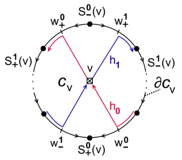
Figure 2.1: Traversing a face vertex $v$ by a ZS-pair $(h_{0},h_{1})$. Note the resulting shapes “Z” of $h_{0}$ (red) and “S” of $h_{1}$ (blue). The paths $h_{\iota}$ may also continue into neighboring faces, beyond $w_{\pm}^{\iota}$, without turning into the face boundary $\partial c$.

In [FiRo16, definitions 2.2 and 5.1] we have introduced formal ZS-pairs and SZS-pairs of paths $(h_{0},h_{1})$ associated to bipolar planar cell complexes and 3-cell templates, respectively. In the following sections we will see how these formal recipes coincide, precisely, with the template table of proposition 2.3, for the traversals of the Sturm paths $(h_{0}^{f},h_{1}^{f})$ through the dynamic cells $c_{v}=W^{u}(v)$ of planar and 3-ball Sturm attractors, in terms of their signed hemisphere decompositions.

More precisely, let us first recall [FiRo16, definition 2.2]; see also [FiRo09]. Let $\mathcal{C}=\bigcup_{v\in\mathcal{E}}c_{v}\subseteq\mathbb{R}^{2}$ be a finite regular planar cell complex with boundary bipolar orientation of the 1-skeleton $\mathcal{C}^{1}$. Let $v$ indicate any source, i.e. the barycenter of a 2-cell face $c_{v}$ in $\mathcal{C}$. By planarity of $\mathcal{C}$ it turns out that the bipolar orientation of $\mathcal{C}^{1}$ defines unique orientation extrema on the boundary circle $\partial c_{v}$ of the 2-cell $c_{v}$. Let $w_{-}^{0}$ be the barycenter on $\partial c_{v}$ of the edge to the right of the minimum, and $w_{+}^{0}$ the edge barycenter to the left of the maximum. Similarly, let $w_{-}^{1}$ be the edge barycenter to the left of the minimum, and $w_{+}^{1}$ to the right of the maximum. See fig. 2.1.

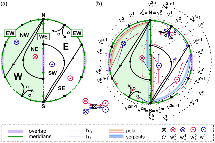
Figure 2.2: The SZS-pair $(h_{0},h_{1})$ in a 3-cell template $\mathcal{C}$, with poles $\mathbf{N},\mathbf{S}$, hemispheres $\mathbf{W},\mathbf{E}$ and meridians $\mathbf{EW},\mathbf{WE}$. Left, (a): schematics of the 3-cell template, as in fig. 1.4. Right, (b): schematics of the SZS-pair. Dashed lines indicate the $h_{\iota}$-ordering of vertices in the closed hemisphere, when $\mathcal{O}$ and the other hemisphere are ignored, according to definition 2.5(i). The actual paths $h_{\iota}$ tunnel, from $w_{-}^{\iota}\in\mathbf{W}$ through the 3-cell barycenter $\mathcal{O}$, and re-emerge at $w_{+}^{\iota}\in\mathbf{E}$, respectively. Note the boundary overlap of the faces $\mathbf{NW},\mathbf{SE}$ of $w_{-}^{1},w_{+}^{0}$ from $v_{-}^{\mu-1}$ to $v_{-}^{\mu^{\prime}+1}$ on the $\mathbf{EW}$ meridian. Similarly, the boundaries of the faces $\mathbf{NE},\mathbf{SW}$ of $w_{-}^{0},w_{+}^{1}$ overlap from $v_{+}^{\nu-1}$ to $v_{+}^{\nu^{\prime}+1}$ along $\mathbf{WE}$.

Definition 2.4.

The paths of labeling bijections $h_{0},h_{1}$: $\{1,\ldots,N\}\rightarrow\mathcal{E}$ are called a ZS-pair $(h_{0},h_{1})$ in the finite, regular, planar and bipolar cell complex $\mathcal{C}=\bigcup_{v\in\mathcal{E}}c_{v}$ if the following three conditions all hold true:

• $h_{0}$ traverses any face $c_{v}$ as $\ldots w_{-}^{0}vw_{+}^{0}\ldots$

• $h_{1}$ traverses any face $c_{v}$ as $\ldots w_{-}^{1}vw_{+}^{1}\ldots$

• both $h_{\iota}$ follow the bipolar orientation of the 1-skeleton $\mathcal{C}^{1}$, if not already defined by (i), (ii).

We call $(h_{0},h_{1})$ an SZ-pair, if $(h_{1},h_{0})$ is a ZS-pair, i.e. if the roles of $h_{0}$ and $h_{1}$ in the rules (i) and (ii) of the face traversals are reversed.

This definition enters the variant of unique SZS-Pairs $(h_{0},h_{1})$, [FiRo16, definition 5.1], associated to 3-cell templates, as follows. See fig. 2.2 for an illustration.

Definition 2.5.

Let $\mathcal{C}=\bigcup_{v\in\mathcal{E}}c_{v}$ be a 3-cell template with oriented 1-skeleton $\mathcal{C}^{1}$, poles $\mathbf{N},\mathbf{S}$, hemispheres $\mathbf{W},\mathbf{E}$, and meridians $\mathbf{EW}$, $\mathbf{WE}$. A path pair $(h_{0},h_{1})$ of labeling bijections $h_{\iota}$: $\{1,\ldots,N\}\rightarrow\mathcal{E}$ is called the SZS-pair assigned to $\mathcal{C}$ if the following two conditions hold.

• The restrictions of range $h_{\iota}$ to $\text{clos }\mathbf{W}$ form an SZ-pair $(h_{0},h_{1})$, in the closed Western hemisphere. The analogous restrictions form a ZS-pair $(h_{0},h_{1})$ in the closed Eastern hemisphere $\text{clos }\mathbf{E}$. See definition 2.4.

• In the notation of fig. 2.2, and for each $\iota=0,1$, the paths $h_{\iota}$ traverse $\mathcal{O}$ in the orders $\ldots w_{-}^{\iota}\mathcal{O}w_{+}^{\iota}\ldots$, respectively.

In [FiRo16, theorem 5.2] we have show that the permutation

(2.24) $$\sigma\mathrel{\mathop{\mathchar 58\relax}}=h_{0}^{-1}\circ h_{1}$$

associated to the SZS-pair $(h_{0},h_{1})$ of any 3-cell template $\mathcal{C}$ is a Sturm meander, i.e. $\sigma$ is a dissipative Morse meander in the sense of [FiRo96]. In particular there exists a dissipative nonlinearity $f$ with hyperbolic equilibria in (1.1), such that the Sturm permutation $\sigma_{f}$ coincides with the formal permutation $\sigma$ associated to (the SZS-pair $(h_{0},h_{1})$ of) the arbitrarily prescribed 3-cell template $\mathcal{C}$:

(2.25) $$\sigma_{f}=\sigma\,.$$

Moreover, $\sigma_{f}$ comes with the associated Sturm global attractor $\mathcal{A}_{f}$, equilibria $\mathcal{E}_{f}$ and the Thom-Smale regular cell complex $\mathcal{C}_{f}=\bigcup_{v\in\mathcal{E}_{f}}c_{v}$, $c_{v}=W^{u}(v)$; see (1.12).

Roughly speaking our main theorem 1.2 claims

(2.26) $$\mathcal{C}_{f}=\mathcal{C}\,,$$

by a cell preserving homeomorphism (1.15). To refine this statement, in view of the signed hemisphere decompositions (2.3), (2.13) of the equilibria $\mathcal{E}_{f}$ into $\mathcal{E}_{\pm}^{j}(v)$, and of the sphere boundaries $\Sigma^{j}(v)=\partial W^{j+1}(v)$ into signed hemispheres $\Sigma_{\pm}^{j}(v)$, we now define a formal hemisphere decomposition $\mathcal{C}^{s}$ on any 3-cell template $\mathcal{C}$. Let $c_{v}$ denote any cell of $\mathcal{C}$, with dimension $i_{v}=\dim c_{v}>0$. If $i_{v}=3$, i.e. for $v=\mathcal{O}$, we define the formal hemispheres $S_{\pm}^{j}(\mathcal{O})$, $j=0,\ldots,3$, analogously to the hemispheres $\Sigma_{\pm}^{j}(\mathcal{O})$ in the translation table (1.20). If $i_{v}=1$, i.e. for edge saddles $v$, we define $S_{+}^{0}(v)$ as the head vertex and $S_{-}^{0}(v)$ as the tail vertex of the edge $c_{v}$ under the bipolar orientation of the 1-skeleton $\mathcal{C}^{1}$. For $i_{v}=2$ faces, we define $S_{-}^{0}(v)$ as the max and $S_{+}^{0}(v)$ as the min vertex on the circle boundary $\partial c_{v}\subseteq\mathcal{C}^{1}$, under its (downward) bipolar orientation; see fig. 2.1. For face sources $v\in\mathbf{E}=\mathrel{\mathop{\mathchar 58\relax}}S_{+}^{2}(\mathcal{O})$, we define the remaining right part of the boundary $\partial c_{v}$ as $S_{-}^{1}(v)$, and the left part as $S_{+}^{1}(v)$. For $v\in\mathbf{W}=\mathrel{\mathop{\mathchar 58\relax}}S_{-}^{2}(\mathcal{O})$, we flip these sides of $S_{\pm}^{1}(v)$, so that $S_{-}^{1}(v)$ is left and $S_{+}^{1}(v)$ right. In summary, the formal hemisphere decomposition $\mathcal{C}^{s}$ of $\mathcal{C}$ consists of $\mathcal{C}$ itself, together with the sign information on

(2.27) $$c_{w}\subseteq S_{\pm}^{j}(v)\,,\quad\text{for any}\quad c_{w}\subseteq\partial c_{v}\,,\,0\leq j<i_{v}\,.$$

In other words, definition 1.1(ii) of bipolarity and meridians in a 3-cell template $\mathcal{C}$ is equivalent to the definition of a formal hemisphere decomposition $\mathcal{C}^{s}$. The translation table for the hemispheres $S_{\pm}^{j}(\mathcal{O})$ is completely analogous to (1.20) with the identification

(2.28) $$S_{\pm}^{j}(\mathcal{O})=\Sigma_{\pm}^{j}(\mathcal{O})\,,$$

$0\leq j\leq 2$. In particular [FiRo16, theorem 4.1] has already identified the dynamic Sturm complex $\mathcal{C}_{f}$ associated to any signed 2-hemisphere template $\mathcal{E}_{\pm}^{j}(v)$, $v\in\mathcal{E}_{f}$, as a 3-cell template $\mathcal{C}^{s}$ with formal hemisphere decomposition $S_{\pm}^{j}(v)$ given by bipolarity, the meridians, and the identification (2.28). The following theorem addresses the converse of this construction.

Theorem 2.6.

Let $\mathcal{C}^{s}=\bigcup_{v\in\mathcal{E}}$ be a 3-cell template with associated formal hemisphere decomposition $S_{\pm}^{j}(v)$ as in (2.27) above. Let $\mathcal{C}_{f}$ be the Sturm dynamic complex (1.12) associated to $\mathcal{C}^{s}$, by the above construction (2.24), (2.25) of an SZS-pair $(h_{0},h_{1})$. Let $\Sigma_{\pm}^{j}(v)$, $v\in\mathcal{E}_{f}$, $0\leq j<i(v)$ be the signed hemisphere decomposition (2.8) on $\mathcal{C}_{f}$.

Then there exists a cell-preserving homeomorphism

(2.29) $$\Phi^{s}\mathrel{\mathop{\mathchar 58\relax}}\qquad\mathcal{C}^{s}=\bigcup\limits_{v\in\mathcal{E}}c_{v}\quad\longrightarrow\quad\bigcup\limits_{v\in\mathcal{E}_{f}}W^{u}(v)=\mathcal{C}_{f}^{s}=\mathcal{A}_{f}$$

with $\Phi^{s}(c_{v})=W^{u}(\Phi^{s}(v))$. Moreover $\Phi^{s}$ is signed, i.e. $\Phi^{s}$ also preserves the signed hemisphere structure

(2.30) $$\Phi^{s}\left(S_{\delta}^{j}(v)\right)=\Sigma_{\delta}^{j}\left(\Phi^{s}(v)\right)\,,$$

for all $v\in\mathcal{E}$, $0\leq j<i_{v}$, and $\delta=\pm$.

In short the SZS-pair $(h_{0},h_{1})$ designs a Sturm global attractor $\mathcal{A}_{f}$ such that the Thom-Smale complex $\mathcal{C}_{f}^{s}$ coincides with the given 3-cell template $\mathcal{C}^{s}$, including the signed hemisphere structure.

Along the proof of the signed realization theorem 2.6, we can also settle the longstanding puzzle on different, not even conjugate, Sturm permutations $\sigma_{f},\sigma_{g}$ with apparently equivalent Sturm attractors $\mathcal{A}_{f}=\mathcal{A}_{g}$ – at least for Sturm 3-balls, and hence also for planar attractors.

Theorem 2.7.

Let $\mathcal{C}_{f}$ and $\mathcal{C}_{g}$ be two Sturm 3-ball dynamic complexes, alias 3-cell templates. Assume there exists a cell-preserving homeomorphism

(2.31) $$\Phi^{s}\mathrel{\mathop{\mathchar 58\relax}}\qquad\mathcal{A}_{f}=\mathcal{C}_{f}^{s}=\bigcup\limits_{v\in\mathcal{E}_{f}}W_{f}^{u}(v)\quad\longrightarrow\quad\bigcup\limits_{v\in\mathcal{E}_{g}}W_{g}^{u}(v)=\mathcal{C}_{g}^{s}=\mathcal{A}_{g}\,,$$

with $\Phi^{s}(W_{f}^{u}(v))=W_{g}^{u}(\Phi^{s}(v))$. Assume $\Phi^{s}$ is signed, i.e. $\Phi^{s}$ also preserves the signed hemisphere decompositions

(2.32) $$\Phi^{s}\left(\Sigma_{\delta}^{j}(v)\right)=\Sigma_{\delta}^{j}\left(\Phi^{s}(v)\right)\,,$$

for all $v\in\mathcal{E}_{f}$, $0\leq j<i(v)$, and $\delta=\pm$.

Then the Sturm permutations of $f$ and $g$ coincide:

(2.33) $$\sigma_{f}=\sigma_{g}\,.$$

Moreover, $\Phi^{s}$ can be chosen to respect all fast unstable manifolds,

(2.34) $$\Phi^{s}\left(W_{f}^{j+1}(v)\right)=W_{g}^{j+1}\left(\Phi^{s}(v)\right)\,,$$

$0\leq j<i(v)$, together with their signed versions.

For an example we refer to [FiRo16, (5.6) and fig. 5.2]. Any cell-preserving homeomorphism $\Phi$, in that example, would have to interchange the respective 2-hemispheres of $\mathcal{O}$,

(2.35) $$\Phi\mathrel{\mathop{\mathchar 58\relax}}\quad\Sigma_{f,\pm}^{2}(\mathcal{O}_{f})\quad\longrightarrow\quad\Sigma_{g,\mp}^{2}(\mathcal{O}_{g})\,.$$

This accounts for different Sturm permutations $\sigma_{f}\neq\sigma_{g}$, which are not trivially conjugate either. See also [FiRo17, fig. 4.6].

3 Planar Sturm attractors

As a prelude to the proof of theorem 2.6 for 3-ball Sturm global attractors we recall the case of planar disks, in theorem 3.1. See [FiRo16, section 2] for details. A central construction, in definition 2.4 above, assigns a ZS-Hamiltonian pair of paths $h_{0},h_{1}$: $\{1,\ldots,N\}\rightarrow\mathcal{E}$ through the vertices $v\in\mathcal{E}$ of the cells $c_{v}$ of a prescribed planar bipolar cell complex $\mathcal{C}$. The construction of $h_{0},h_{1}$ ensures that the permutation $\sigma$:= $h_{0}^{-1}\circ h_{1}\in S_{N}$ is Sturm, $\sigma=\sigma_{f}$ and hence defines a Sturm meander $\mathcal{M}_{f}$. Moreover, the associated Sturm global attractor $\mathcal{A}_{f}$ is planar with Thom-Smale cell complex $\mathcal{C}_{f}$ as prescribed by $\mathcal{C}$. See theorem 3.1. We then refine the analysis of the cell complex equality $\mathcal{C}_{f}=\mathcal{C}$, in the planar case. In fact $\mathcal{C}_{f}=\mathcal{C}$ is understood in terms of a cell-to-cell homeomorphism $\Phi$: $\mathcal{C}\rightarrow\mathcal{C}_{f}$. We refine this to a signed homeomorphism $\Phi^{s}$: $\mathcal{C}^{s}\rightarrow\mathcal{C}_{f}^{s}$ between signed cell complexes. In other words, $\Phi^{s}(S_{\delta}^{j}(v))=\Sigma_{\delta}^{j}(\Phi^{s}(v))$ maps corresponding hemispheres of $\mathcal{C}^{s}$ and $\mathcal{C}_{f}^{s}$ onto each other, for all equilibria $v$, signs $\delta=\pm$, and dimensions $0\leq j<i(v)$; see (3.2) and corollary 3.2. In particular we show how the disk orientations of the planar embedding $\mathcal{C}\subseteq\mathbb{R}^{2}$, together with the bipolar orientation of the 1-skeleton $\mathcal{C}^{1}$, already fix a signed hemisphere structure of $\mathcal{C}^{s}$, and hence determine the boundary orders $h_{\iota}^{f}=h_{\iota}$ and the Sturm permutation $\sigma_{f}=h_{0}^{-1}h_{1}$ uniquely. See (3.9)–(3.13). For a topological disk $\mathcal{C}$, we recall how the remaining freedom of sign choices when passing to $\mathcal{C}^{s}$ amounts to trivially equivalent global attractors $\mathcal{A}_{f}=\mathcal{C}_{f}$, under $x\mapsto 1-x$ and $u\mapsto-u$, once the target sink equilibria of the one-dimensional fast unstable manifolds $W^{1}(v)$ have been fixed, for all $i=2$ source equilibria $v$.

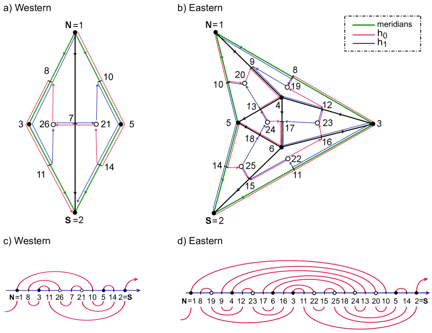
Figure 3.1: The closed hemisphere Thom-Smale complexes, alias topological disk attractors, of the 3-cell octahedron from fig. 1.3. Western hemisphere (a), and Eastern hemisphere (b). See (c), (d) for the associated meanders, respectively. Vertex annotations, viz. equilibrium labels, correspond to fig.1.3.

We first consider planar Sturm global attractors $\mathcal{A}_{f}$ and complexes $\mathcal{C}$ which are topological disks. By this we mean that $\mathcal{A}_{f}$, $\mathcal{C}$ are allowed to contain several sources of Morse index $i=2$, alias faces, but $\mathcal{A}_{f}$, $\mathcal{C}$ are homeomorphic to the standard closed disk. We recall definition 2.1 of the signed hemisphere template $\mathcal{E}_{\pm}^{j}(v)$ of $\mathcal{A}_{f}$, according to equilibria in the hemisphere decomposition $\Sigma_{\pm}^{j}(v)$ of $\partial W^{u}(v)$, for all equilibria $v\in\mathcal{E}_{f}$ and $0\leq j<i(v)$. In [FiRo16, theorem 2.4] we proved the following theorem.

Theorem 3.1.

• linebreak

• Let $(h_{0},h_{1})$ be the ZS-pair of a given planar bipolar topological disk complex $\mathcal{C}\subseteq\mathbb{R}^{2}$ with poles $\mathbf{N}$, $\mathbf{S}$ on the circular boundary of $\mathcal{C}$. Then the Sturm permutation $\sigma_{f}=\sigma$:= $h_{0}^{-1}h_{1}$ defines a topological disk Sturm global attractor $\mathcal{A}_{f}$ with dynamic complex $\mathcal{C}_{f}=\mathcal{C}$, and hence a unique signed hemisphere template $\mathcal{E}_{\pm}^{j}(v)$.

• Conversely, let $\mathcal{E}_{\pm}^{j}(v)$ be the signed hemisphere template of a given planar Sturm global attractor $\mathcal{A}_{f}$. Then $\mathcal{E}_{\pm}^{j}(v)$ defines a unique bipolar orientation of the planar Thom-Smale complex $\mathcal{C}_{f}$ of $\mathcal{A}_{f}$, and hence a unique ZS-pair $h_{\iota}$:= $h_{\iota}^{f}$, $\iota=0,1$.

See fig. 3.1(b) for an illustration of theorem 3.1, featuring the ZS-pair $(h_{0},h_{1})$ for the given orientation of the Eastern hemisphere part of the solid octahedron from fig. 1.3. In fig. 3.1(a) the SZ-pair $(h_{0},h_{1})$ is illustrated for the Western hemisphere of the same example.

Since theorem 3.1 will play a central role in our proof of theorems 2.6 and 2.7, let us comment on the precise interpretation of the equality $\mathcal{C}=\mathcal{C}_{f}$ here; see [FiRo08] for further details. As in the 3-ball case of theorem 2.6, equality is understood in the sense of a cell preserving homeomorphism

(3.1) $$\Phi^{s}\mathrel{\mathop{\mathchar 58\relax}}\qquad\mathcal{C}=\bigcup\limits_{v\in\mathcal{E}}c_{v}\quad\longrightarrow\quad\bigcup\limits_{v\in\mathcal{E}_{f}}W^{u}(v)=\mathcal{C}_{f}=\mathcal{A}_{f}$$

with $\Phi^{s}(c_{v})=W^{u}(v)$, which also preserves the signed hemisphere structure

(3.2) $$\Phi^{s}\left(S_{\delta}^{j}(v)\right)=\Sigma_{\delta}^{j}\left(\Phi^{s}(v)\right)\,,$$

for all $v\in\mathcal{E}$, $0\leq j<i_{v}$, and $\delta=\pm$. First, this requires a bijective identification

(3.3) $$\Phi^{s}\mathrel{\mathop{\mathchar 58\relax}}\qquad\mathcal{E}\quad\longrightarrow\quad\mathcal{E}_{f}\,,$$

for the restriction of $\Phi^{s}$ to the barycenters $v\in\mathcal{E}$ of the cells $c_{v}\in\mathcal{C}$. Recalling [FiRo08, lemma 5.2], this identification is defined by the ZS-pair $(h_{0},h_{1})$ in $\mathcal{E}$ and the boundary orders $(h_{0}^{f},h_{1}^{f})$ in $\mathcal{E}_{f}$ as

(3.4) $$\Phi^{s}\mathrel{\mathop{\mathchar 58\relax}}=h_{\iota}^{f}\circ h_{\iota}^{-1}\,.$$

Since $h_{0}^{-1}\circ h_{1}=\sigma=\sigma_{f}=(h_{0}^{f})^{-1}\circ h_{1}^{f}$, the two choices $\iota=0,1$ define the same bijection $\Phi^{s}$ in (3.3), (3.4). We therefore use the same symbol $v$ to denote $v\in\mathcal{E}$ and $\Phi^{s}(v)\in\mathcal{E}_{f}$. With this convention we obtain

(3.5) $$h_{\iota}=h_{\iota}^{f}$$

for $\iota=0,1$.

In [FiRo08, lemma 5.3] we have shown that the vertex identification (3.3), (3.4) between $\mathcal{C}$ and $\mathcal{C}_{f}$ already defines an isomorphism between the filled graph $G_{2}$ of $\mathcal{C}$ and the (unsigned) connection graph $\mathcal{H}_{f}$ of $\mathcal{C}_{f}$. Here the filled graph $G_{2}$ of $\mathcal{C}$ is augmented by the edges from any face center $v$, of 2-dimensional cells $c_{v}$ in $\mathcal{C}$, to all saddles $w$ of edges $c_{w}\subseteq\partial c_{v}$, in addition to the bipolar 1-skeleton $\mathcal{C}^{1}$. Sometimes $G_{2}$ is called the quadrangulation of $\mathcal{C}^{1}$ to emphasize the partitions of $c_{v}$ into quadrangles. The graph isomorphism preserves orientation on $\mathcal{C}^{1}$. By transitivity and cascading of heteroclinic connectivity in the Sturm attractor $\mathcal{A}_{f}=\mathcal{C}_{f}$ we also conclude

(3.6) $$\dim c_{v}=\dim W^{u}(v)=i(v)=i_{v}\,,$$

i.e. the vertex identification (3.3) preserves cell dimension. More precisely, the graph isomorphism $\Phi^{s}$: $G_{2}\rightarrow\mathcal{H}_{f}$ ensures the left equivalence in

(3.7) $$c_{w}\subseteq\partial c_{v}\quad\Longleftrightarrow\quad v\leadsto w\quad\Longleftrightarrow\quad W^{u}(w)\subseteq\partial W^{u}(v)\,.$$

The right equivalence follows from Morse-Smale transversality in the Thom-Smale complex, as we recall from the introduction. This allows us to define the homeomorphism $\Phi^{s}$ by induction over the cell dimensions $i(v)$ as follows.

The identification of $0$-cells $c_{v}$, alias sink vertices $i(v)=0$, takes care of the case $i(v)=0$. Once the homeomorphism $\Phi^{s}$: $\mathcal{C}^{i-1}\rightarrow\mathcal{C}_{f}^{i-1}$ has been constructed for the $(i-1)$-skeleta, $i\geq 1$, we can define the extension

(3.8) $$\Phi^{s}\mathrel{\mathop{\mathchar 58\relax}}\qquad\mathcal{C}^{i}\quad\longrightarrow\quad\mathcal{C}_{f}^{i}\,,$$

separately on each closed cell $\overline{c}_{v}$ of dimension $i(v)=i$. Indeed, we may simply extend $\Phi^{s}$, already defined on the sphere boundary $S^{i-1}(v)=\partial c_{v}\subseteq\mathcal{C}^{i-1}$ of any regular cell $\overline{c}_{v}\subseteq\mathcal{C}^{i}$, radially inwards towards the cell center $v$.

The construction of a signed homeomophism $\Phi^{s}$, however, requires a little extra care. On 1-cell edges $c_{w}$ of the bipolar 1-skeleton $\mathcal{C}^{1}$ we observe how the graph isomorphism $\Phi^{s}$ in (3.3), (3.4) maps tails $S_{-}^{0}(w)$ and heads $S_{+}^{0}(w)$ of the bipolar orientation to the signed hemi“sphere” boundaries $\Sigma_{-}^{0}(w)$ and $\Sigma_{+}^{0}(w)$ of the edge $W^{u}(w)$, respectively. See our definition of $S_{\pm}^{j}$ above (2.27). Indeed, we first note that both $h_{\iota}^{f}$ traverse the sink equilibrium $\Sigma_{-}^{0}(w)$ before $\Sigma_{+}^{0}(w)>w>\Sigma_{-}^{0}(w)$, simply because both $h_{\iota}^{f}$ proceed according to the boundary order at $x=\iota=0,1$.

We show next how each of the paths $h_{\iota}$ in $\mathcal{C}$, likewise, traverses the tail vertex $S_{-}^{0}(w)$ before the head vertex $S_{+}^{0}(w)$. Indeed the ZS-rules of definition 2.4 for the ZS-pair $(h_{0},h_{1})$ of Hamiltonian paths in $G_{2}$ ensure that both $h_{\iota}$ traverse the vertex $S_{-}^{0}(w)$ before $S_{+}^{0}(w)$. In fact, each $h_{\iota}$ defines an extension of the partial bipolar order on $\mathcal{C}^{1}\cap\mathcal{E}$ to a total order of all vertices $\mathcal{E}$ of $G_{2}$. To see this we just observe that each $h_{\iota}$ defines a polar Jordan curve from $\mathbf{N}$ to $\mathbf{S}$ in the planar complex $\mathcal{C}$; see also fig. 2.1. Therefore $\Phi^{s}$ is signed, automatically, on the 1-skeleta $\mathcal{C}^{1}$ and $\mathcal{C}_{f}^{1}$.

It remains to understand why $\Phi^{s}$ is also signed on each face closure $\overline{c}_{v}\rightarrow\text{clos }W^{u}(v)$, for $i=2$ sources $v$. Again we note how both $h_{\iota}^{f}$ traverse $\Sigma_{-}^{0}(v)$ before, and $\Sigma_{+}^{0}(v)$ after, any other equilibrium in $\text{clos }W^{u}(v)$. The same holds true for the paths $h_{\iota}$ in the closed 2-cell $\overline{c}_{v}$, with respect to the boundary minimum $S_{-}^{0}(v)$ and the boundary maximum $S_{+}^{0}(v)$, respectively, under the bipolar orientation of the 1-skeleton $\mathcal{C}^{1}$. Therefore $\Phi^{s}$ maps the vertices $S_{\delta}^{0}(v)$ to the equilibria $\Sigma_{\delta}^{0}(v)$, respectively, for $\delta=\pm$.

Our choice of the ZS-pair $(h_{0},h_{1})$ for the labeling maps $h_{\iota}$, in the cell complex $\mathcal{C}$, and the identification $h_{\iota}=h_{\iota}^{f}$ in (3.4), (3.5) further imply

(3.9) $$\Phi^{s}\left(S_{\delta}^{1}(v)\right)=\Sigma_{\delta}^{1}(v)\,,$$

for any $i=2$ source $v$ and any $\delta=\pm$. Indeed, the boundary order $h_{0}^{f}$ traverses $w(+-)$, and hence all equilibria in $\Sigma_{-}^{1}(v)$, before the face center $v$; see proposition 2.3. Similarly, $h_{0}^{f}$ traverses $w(-+)$, as well as all other equilibria in $\Sigma_{+}^{1}(v)$, after $v$. In the exact same way, the abstract path $h_{0}$ traverses all vertices in the right boundary $S_{-}^{1}(v)$ of the face $c_{v}$ before, and the left boundary $S_{+}^{1}(v)$ after, the face center $v$ itself. This proves (3.9). It also shows that the homeomorphism $\Phi^{s}$, defined by radial extension above, is already a signed homeomorphism, i.e. $\Phi^{s}$: $\mathcal{C}\rightarrow\mathcal{C}_{f}$ preserves the signed hemisphere decompositions of $\mathcal{C}$ and $\mathcal{C}_{f}$. It is useful to rethink the above observations, based on $h_{1}=h_{1}^{f}$ instead $h_{0}=h_{0}^{f}$ – with identical results.

Next consider two planar Sturm attractors $\mathcal{A}_{f}$ and $\mathcal{A}_{g}$ which are topological disks. Suppose $\mathcal{A}_{f}$ and $\mathcal{A}_{g}$ possess the same signed hemisphere decompositions $\Sigma_{f,\pm}^{j}(v)$, $\Sigma_{g,\pm}^{j}(v)$ of their Sturm complexes $\mathcal{C}_{f}$ and $\mathcal{C}_{g}$. By this we mean a bijection $\mathcal{E}_{f}\rightarrow\mathcal{E}_{g}$ of equilibria $v_{f}\mapsto v_{g}$, with isomorpic connection graphs $\mathcal{H}_{f}\cong\mathcal{H}_{g}$, such that the signed zero numbers coincide,

(3.10) $$z(w_{f}-v_{f})=z(w_{g}-v_{g})\,,$$

whenever $v_{f}\leadsto w_{f}$, alias $v_{g}\leadsto w_{g}$. By the above arguments, we then have a signed homeomorphism

(3.11) $$\Phi^{s}\mathrel{\mathop{\mathchar 58\relax}} \mathcal{C}_{f}^{s}\longrightarrow\mathcal{C}_{g}^{s}$$

$$\Phi^{s}\mathrel{\mathop{\mathchar 58\relax}}= \Phi_{g}^{s}\circ\left(\Phi_{f}^{s}\right)^{-1}$$

of their signed Sturm complexes, which preserves the respective signed hemisphere decompositions:

(3.12) $$\Phi^{s}\left(\Sigma_{f,\pm}^{j}(v_{f})\right)=\Sigma_{g,\pm}^{j}(v_{g})\,.$$

Moreover, (3.5) implies $h_{\iota}^{f}=h_{\iota}^{g}$, for $\iota=0,1$, and hence the Sturm permutations $\sigma=h_{0}^{-1}\circ h_{1}$ coincide,

(3.13) $$\sigma_{f}=\sigma_{g}\,.$$

In this sense, theorems 2.6 and 2.7 hold true for planar Sturm attractors which are topological disks.

Let us add a word about orientation. Suppose we had chosen an SZ-pair $(h_{0},h_{1})$ in the planar topological disk $\mathcal{C}$, instead of a ZS-pair. Then we should define the left, rather than the right, boundary of all faces $c_{v}$ to be $S_{-}^{1}(v)$. The right boundaries would then become $S_{+}^{1}(v)$, instead. By the above arguments, the homeomorphism $\Phi^{s}$ would then remain signed. Effectively this amounts to a homeomorphic description of the Sturm complex $\mathcal{C}_{f}$ by a planar complex of the opposite orientation. Comparing the separated Western and Eastern hemispheres of the solid octahedron in fig. 1.3, as depicted in fig. 3.1(a), (b), the hemisphere descriptions differ by precisely this orientation reversal. This is due to the fact that we present both hemispheres $\Sigma_{\pm}^{2}(\mathcal{O})$ of $\Sigma^{2}(\mathcal{O})$ in the same coordinate frame. Note however, how the identified meridians $\mathbf{WE}=\Sigma_{+}^{1}(\mathcal{O})$ and $\mathbf{EW}=\Sigma_{-}^{1}(\mathcal{O})$ of fig. 1.3 and table (1.20) entirely consist of edges in $\Sigma_{+}^{1}(v)$ and $\Sigma_{-}^{1}(v)$, respectively, in either planar orientation. In [FiRo16, fig. 5.2], we have presented an example of orientation reversal in a Sturm 3-ball.

We can now extend theorem 3.1 to general planar Sturm attractors $\mathcal{A}_{f}$ which are not topological disks. Such attractors consists of a linear chain of a number $d\geq 0$ of topological disks with intermediate one-dimensional chains, glued on. This possibly includes a prepended and/or appended one-dimensional spike. The chains consist of alternating sinks and saddles, each chain with a first and, possibly identical, last sink.

For a single topological disk, the orientation reversal of the planar embedding of a single 2-cell face reverses the orientation of all other cells. For several disk components, $d>1$, we may choose the orientation of each cell, individually. In general, this will lead to cell-homeomorphic planar Sturm attractors $\mathcal{A}_{f}$ with different Sturm permutations $\sigma_{f}$. Fixing the signed hemisphere decomposition, alias the ZS-rule for face traversing pairs $(h_{0},h_{1})$, alias the right/left rule for $S_{\pm}^{1}(v)$ in cell faces, will still determine the signed Sturm complex $\mathcal{C}_{f}^{1}(v)$ and the Sturm permutation $\sigma_{f}$ uniquely.

These remarks prove the following variant of theorem 3.1, in terms of signed planar cell complexes.

Corollary 3.2.

• linebreak

• Let $(h_{0},h_{1})$ be the ZS-pair of any given planar bipolar complex $\mathcal{C}^{s}\subseteq\mathbb{R}^{2}$ with poles $\mathbf{N}$, $\mathbf{S}$ on the boundary of $\mathcal{C}_{f}$. This identifies $\mathcal{C}$ as a signed complex $\mathcal{C}^{s}$; see (2.27). Then the Sturm permutation $\sigma_{f}=\sigma$:= $h_{0}^{-1}h_{1}$ defines a unique signed Sturm complex

  (3.14) $$\mathcal{C}_{f}^{s}=\mathcal{C}^{s}\,,$$

  in the sense of (2.3), (2.14). Equality in (3.14) is understood by a signed homeomorphism $\Phi^{s}$ as in (3.1), (3.2) above.

• Conversely, let $\mathcal{C}_{f}^{s}$ be the signed Sturm complex of a given planar Sturm attractor $\mathcal{A}_{f}$. Then the signed hemisphere decomposition $\mathcal{C}_{f}^{s}$ defines a planar embedding of $\mathcal{C}_{f}^{s}$, with unique orientation of each disk component of $\mathcal{C}_{f}^{s}$, such that the boundary orders $h_{\iota}$:= $h_{\iota}^{f}$, $\iota=0,1$ are a ZS-pair.

We conclude this section by recalling the role of the fast unstable manifolds $W^{uu}(v)=W^{1}(v)$ of $i=2$ sources $v$ in 2-cells $c_{v}=W^{u}(v)$. Their role is usually ignored in the study of Thom-Smale dynamic complexes. Our goal is to clarify the extent to which these fast unstable manifolds already determine the sign information in the signed Sturm complex $\mathcal{C}_{f}^{s}$, given just the Sturm complex $\mathcal{C}_{f}$ itself. Since $z(\cdot-v)=0_{\pm}$ on $W^{1}(v)\smallsetminus\{v\}$, these manifolds are heteroclinic orbits

(3.15) $$v\leadsto\Sigma_{\pm}^{0}(v)\,;$$

see proposition 2.2(iii). In particular their targets identify the bipolar extrema $\Sigma_{\pm}^{0}(v)$ in the circular cell boundary $\partial W^{u}(v)=\partial c_{v}$, up to sign. Flipping this sign in one single 2-cell flips all signs, in unison. This defines the bipolar orientation on the 1-skeleton $\mathcal{C}_{f}^{1}$, up to global sign reversal.

In a planar Sturm attractor it only remains to determine the 1-hemispheres $\Sigma_{\pm}^{1}(v)$, for a complete specification of the signed Sturm complex $\mathcal{C}_{f}^{s}$. For the case $d=1$ of a single topological disk, only, this follows globally from the bipolar orientation, up to a global simultaneous swap of all $\Sigma_{+}^{1}(v)$ with their respective counterparts $\Sigma_{-}^{1}(v)$.

Both the global reversal of the bipolar orientation and the global orientation flip of the planar embedding can be achieved by the trivial equivalences $x\mapsto 1-x$, $u\mapsto-u$; see the introduction and [FiRo16, corollary 2.5]. In conclusion, the Sturm complex $\mathcal{C}_{f}$ determines its signed version $\mathcal{C}_{f}^{s}$ uniquely, up to trivial equivalences, for the case $d=1$ of a single topological disk. By corollary 3.2, this determines the realizing Sturm permutation $\sigma=\sigma_{f}$ of the prescribed (unsigned) Sturm complex $\mathcal{C}=\mathcal{C}_{f}$ uniquely, up to a flip conjugation $k\sigma k$ and taking inverses, once the target equilibria of the fast unstable manifolds $W^{1}(v)$ are specified.

This planar result neither extends to the case $d\geq 2$ of planar Sturm attractors $\mathcal{A}_{f}$ with multiple topological disk components, nor to 3-ball Sturm attractors.

4 Noses and scoops

In this section we study noses $\{v_{1},v_{2}\}\in\mathcal{E}$ of concrete and abstract Sturm permutations $\sigma_{f}=\sigma$. Abstractly, let $h_{\iota}$: $\{1,\ldots,N\}\rightarrow\mathcal{E}$ be labeling maps such that $\sigma$:= $h_{0}^{-1}h_{1}$ is Sturm. Then we call the pair $\{v_{1},v_{2}\}$ a nose if the elements $v_{j}$ are adjacently labeled by both maps $h_{\iota}$, i.e.

(4.1) $$|h_{\iota}^{-1}(v_{1})-h_{\iota}^{-1}(v_{2})|=1\,,$$

for $\iota=0,1$.

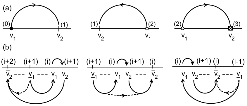
Figure 4.1: Upper arc noses $\{v_{1},v_{2}\}$, such that $h_{0}^{-1}(v_{2})=h_{0}^{-1}(v_{1})+1$. (a) All cases with Morse numbers $i_{v_{j}}\leq 3$ (in parentheses). Note how the meander $\mathcal{M}$ crosses the horizontal $h_{1}$-axis upwards, at even Morse numbers $(i_{v_{1}})$, and downwards at odd $(i_{v_{2}})$. (b) Configurations with $i(v_{2})=i(v_{1})+1$, including $h_{0}$-predecessors $\underline{v}_{1}$ of $v_{1}$ and successors $\overline{v}_{2}$ of $v_{2}$. Lower shortcut arcs in $\check{\mathcal{M}}$, from $\underline{v}_{1}$ to $\overline{v}_{2}$ after retraction of the nose $\{v_{1},v_{2}\}$ are dashed.

We exclude the polar cases of $h_{\iota}^{-1}(v_{1})$ or $h_{\iota}^{-1}(v_{2})$ in $\{1,N\}$ just for simplicity of notation in the nose retractions below. The naming comes from the resulting arc configuration in the meander $\mathcal{M}$ associated to $\sigma$. See also [FiRo99]. See fig. 4.1 for the list of upper nose examples, i.e. $\mathcal{M}$-arcs above the horizontal $h_{1}$-axis, with Morse numbers $i\leq 3$. Without loss of generality we fix

(4.2) $$h_{0}^{-1}(v_{2})=h_{0}^{-1}(v_{1})+1\,.$$

By (1.25), (1.26) the More numbers $i_{v_{j}}$ are also adjacent,

(4.3) $$|i(v_{1})-i(v_{2})|=1\,,$$

and of the opposite even/odd parity compared to either label $h_{\iota}^{-1}(v_{j})$. The meander itself crosses the horizontal $h_{1}$-axis upwards, at odd labels, and downwards, at even labels.

A nose retraction passes from $h_{\iota},\sigma$ to $\check{h}_{\iota},\check{\sigma}$, simply skipping a nose $\{v_{1},v_{2}\}$ and its labels. Thus $\check{h}_{\iota}$: $\{1,\ldots,N-2\}\rightarrow\check{\mathcal{E}}$:= $\mathcal{E}\smallsetminus\{v_{1},v_{2}\}$ and

(4.4) $$\check{\sigma}\mathrel{\mathop{\mathchar 58\relax}}=\check{h}_{0}^{-1}\circ\check{h}_{1}\,.$$

The associated meander $\check{\mathcal{M}}$ of $\check{\sigma}$ connects the intersection $\underline{v}_{1}$:= $h_{0}(h_{0}^{-1}(v_{1})-1)$ of the $v_{1}$-predecessor to the $v_{2}$-successor $\overline{v}_{2}$:= $h_{0}(h_{0}^{-1}(v_{2})+1)$ by a direct arc of $\check{\mathcal{M}}$, in the half plane opposite to the arc $v_{1}v_{2}$. The shortcut $\check{h}_{0}$: $\ldots\underline{v}_{1}\overline{v}_{2}\ldots$ is dashed in fig. 4.1(b).

In proposition 4.1 below we show that nose retractions do not affect the Sturm property, Morse indices, or signed zero numbers of the remaining elements. We caution the reader, however, that the remaining heteroclinic orbits of the connection graph $\mathcal{H}$ may well be affected. In definition 4.2 we introduce certain sequences of successive nose retractions, called scoops. In proposition 4.3, these scoops reduce permutations $\sigma$ of 3-meander templates to Sturm permutations $\sigma_{\pm}$ of planar Sturm attractors $\mathcal{A}_{\pm}$. In section 5, we will identify $\mathcal{A}_{\pm}$ as the closed hemispheres of the Sturm 3-ball attractor of $\sigma$ itself.

Proposition 4.1.

Let $\sigma\in S_{N}$ be any Sturm permutation, and let $\check{\sigma}\in S_{N-2}$ arise by nose retraction of $\{v_{1},v_{2}\}$ from $\sigma$; see (4.4).

Then $\check{\sigma}$ is again a Sturm permutation. The Morse indices $i_{v}$ and the signed zero numbers $z_{wv}$ of $v\neq w$ are all inherited from $\sigma$, without any change, for $v,w\in\check{\mathcal{E}}$:= $\mathcal{E}\smallsetminus\{v_{1},v_{2}\}$.

Proof..

Without loss of generality, and to simplify language, suppose $\{v_{1},v_{2}\}$ is an upper arc nose. Else apply the trivial equivalence $u\mapsto-u$, which rotates all Sturm meanders by $180^{\circ}$. By the labeling (4.2) this implies $i$:= $i_{v_{1}}$ is even and $i_{v_{2}}=i_{v_{1}}\pm 1$ is odd.

We first show how $\check{\sigma},\check{\mathcal{M}}$ define a meander. In the meander $\mathcal{M}$ associated to $\sigma$ we only consider the case of a right oriented, and hence right turning, upper nose arc from $v_{1}$ to $v_{2}$. Then $i_{v_{2}}=i_{v_{1}}+1$. The other case, $i_{v_{2}}=i_{v_{1}}-1$, is analogous and will be omitted. See fig. 4.1(b) for the resulting arc configurations and the Morse numbers of $h_{0}$: $\ldots\underline{v}_{1}v_{1}v_{2}\overline{v}_{2}\ldots$. The nose vertices $v_{1}$ and $v_{2}=h_{1}(h_{1}^{-1}(v_{1})+1)$ are also $h_{1}$-adjacent, by definition (4.1). The dashed lower arc shortcuts $\check{h}_{0}$: $\ldots\underline{v}_{1}\overline{v}_{2}\ldots$ which skip the retracted nose $\{v_{1},v_{2}\}$, therefore define a meander $\check{M}$. In particular the permutation $\check{\sigma}$ defined by $\check{\mathcal{M}}$ is a meander. Moreover $\check{\sigma}$ is dissipative by our exclusion of polar noses $\{v_{1},v_{2}\}$.

To show preservation of Morse numbers under nose retraction we again consult the three cases of fig. 4.1(b), only. We compare the recursion (1.25) for the passage from $i_{\overline{v}_{1}}$ to $i_{\overline{v}_{2}}$ before and after nose retraction of $\{v_{1},v_{2}\}$. By induction from $j=0$ to $j_{1}=h_{0}^{-1}(\overline{v}_{1})$, the Morse numbers $i_{\overline{v}_{1}}$ coincide. By inspection of fig. 4.1(b), the resulting Morse numbers $i_{\overline{v}_{2}}=i_{h_{0}(j_{1}+3)}=i_{\check{h}_{0}(j_{1}+1)}$ coincide in all cases. This proves preservation of Morse numbers. In particular $\check{\sigma}$ is Morse, as $\sigma$ is, which proves $\check{\sigma}$ is Sturm.

We prove preservation of the signed zero numbers $\check{z}_{vw}=z_{vw}$ under nose retraction of $\{v_{1},v_{2}\}$, next. Since nose retraction does not alter the $h_{0}$-order $<_{0}$ of the remaining vertices in $\check{\mathcal{E}}$, it is sufficient to prove preservation of the unsigned zero numbers. In view of the explicit recursions (2.5) and preservation of Morse numbers, it is sufficient to prove

(4.5) $$\check{z}_{\overline{v}_{2}w}-\check{z}_{\underline{v}_{1}w}=z_{\overline{v}_{2}w}-z_{\underline{v}_{1}w}$$

for $h_{0}$: $\ldots\underline{v}_{1}v_{1}v_{2}\overline{v}_{2}\ldots$ and any $w<_{0}v_{1}$. Here $\check{z}$ refers to $\check{h}_{\iota}$, $\check{\sigma}$ after nose retraction of $\{v_{1},v_{2}\}$. With the notation $k,j_{1}$ for $h_{0}^{-1}(w)$, $h_{0}^{-1}(v_{1})$, and the abbreviations $\zeta_{j},\check{\zeta}_{j}$ and $s_{j}$ for unsigned $z_{h_{0}(j)h_{0}(k)}$, $\check{z}_{h_{0}(j)h_{0}(k)}$, and $\tfrac{1}{2}\text{sign}(\sigma^{-1}(j)-\sigma^{-1}(k))$, respectively, claim (4.5) reads

(4.6) $$\check{\zeta}_{j_{1}}-\check{\zeta}_{j_{1}-1}=\zeta_{j_{1}+2}-\zeta_{j_{1}-1}\,.$$

To prove claim (4.6), we first note that recursion (2.5) asserts

(4.7) $$\zeta_{j+1}-\zeta_{j}=(-1)^{j+1}\left(s_{j+1}-s_{j}\right)\,.$$

Note $s_{j_{1}+1}=s_{j_{1}}$ for the adjacent nose equilibria $v_{2}=h_{0}(j_{1}+1)$ and $v_{1}=h_{0}(j_{1})$. Summing (4.7) from $j=j_{1}-1$ to $j=j_{1}+1$ therefore implies

(4.8) $$\zeta_{j_{1}+2}-\zeta_{j_{1}-1}=$$

$$\quad=(-1)^{j_{1}}\left(s_{j_{1}}-s_{j_{1}-1}\right)+(-1)^{j_{1}+1}\left(s_{j_{1}+1}-s_{j_{1}}\right)+(-1)^{j_{1}+2}\left(s_{j_{1}+2}-s_{j_{1}+1}\right)=$$

$$\quad=(-1)^{j_{1}}\left(-s_{j_{1}-1}+2s_{j_{1}}-2s_{j_{1}+1}+s_{j_{1}+2}\right)=$$

$$\quad=(-1)^{j_{1}}\left(s_{j_{1}+2}-s_{j_{1}-1}\right)=$$

$$\quad=\check{\zeta}_{j_{1}}-\check{\zeta}_{j_{1}-1}\,.$$

Here we have used $\check{s}_{j_{1}-1}=s_{j_{1}-1}$ and $\check{s}_{j_{1}}=s_{j_{1}+2}$ in the last equality. This proves signed invariance of signed zero numbers under nose retraction, and also proves the proposition. ∎

From now on, and for the remaining paper, we return to a 3-meander template $\mathcal{M}$ with associated Sturm permutation $\sigma_{f}=\sigma$, Sturm attractor $\mathcal{A}_{f}$, Sturm complex $\mathcal{C}_{f}$, and boundary orders $h_{\iota}^{f}$ at $x=\iota=0,1$. See definition 1.3. Our first task is to work towards identifying $\mathcal{A}_{f}$ as a Sturm 3-ball, in theorem 5.1 below. As candidates ${\mathcal{E}^{\prime}}_{\pm}^{j}$ for the equilibrium sets $\mathcal{E}_{\pm}^{j}$ in the signed hemisphere decomposition $\Sigma_{\pm}^{j}$ of the 2-sphere $\partial W^{u}(\mathcal{O})$, we define the following sets of vertices $\mathcal{E}$, alias equilibria $\mathcal{E}_{f}$:

(4.9) $${\mathcal{E}^{\prime}_{-}}^{0} \mathrel{\mathop{\mathchar 58\relax}}=\{h_{\iota}^{f}(1)\}\,,\quad{\mathcal{E}^{\prime}_{+}}^{0}\mathrel{\mathop{\mathchar 58\relax}}=\{h_{\iota}^{f}(N)\}\,;$$

$${\mathcal{E}^{\prime}_{-}}^{1} \mathrel{\mathop{\mathchar 58\relax}}=\{v_{-}^{1},v_{-}^{2},\ldots,v_{-}^{2m-1}\}\,,\quad{\mathcal{E}^{\prime}_{+}}^{1}\mathrel{\mathop{\mathchar 58\relax}}=\{v_{+}^{1},v_{+}^{2},\ldots,v_{+}^{2n-1}\}\,;$$

$${\mathcal{E}^{\prime}}^{j} \mathrel{\mathop{\mathchar 58\relax}}=\bigcup\limits_{k\leq j,\,\delta=\pm}{\mathcal{E}^{\prime}_{\delta}}^{k}\,,\quad\text{clos }{\mathcal{E}^{\prime}_{\delta}}^{j}\mathrel{\mathop{\mathchar 58\relax}}={\mathcal{E}^{\prime}_{\delta}}^{j}\cup{\mathcal{E}^{\prime}}^{j-1}\,;$$

$${\mathcal{E}^{\prime}_{\delta}}^{2} \mathrel{\mathop{\mathchar 58\relax}}=\{v\in\mathcal{E}\smallsetminus{\mathcal{E}^{\prime}}^{1}\,|\,v\neq\mathcal{O}\,,\,\,\delta\mathcal{O}<\delta v\ \text{ at }\ x=1\}\,.$$

Here $j=0,1,2$ and $\delta=\pm$.

Definition 4.2.

We define the East scoop $\mathcal{M}_{-}$ with scooped Sturm permutation $\sigma_{-}$:= $(\check{h}_{0})^{-1}\circ\check{h}_{1}$ as the result of the removal of $\mathcal{O}\cup{\mathcal{E}^{\prime}_{+}}^{2}$, by successive nose retraction. This leads to the replacement of the meander part

(4.10) $$h_{0} \mathrel{\mathop{\mathchar 58\relax}}\quad v_{-}^{0}\ldots v_{-}^{\mu}\ldots v_{-}^{\mu^{\prime}}w_{-}^{1}\ldots v_{-}^{2m-1}\ldots w_{-}^{0}\mathcal{O}w_{+}^{0}\ldots v_{+}^{2n-1}\ldots w_{+}^{1}v_{+}^{\nu^{\prime}}\ldots v_{+}^{\nu}\ldots v_{+}^{0}$$

by

$$\check{h}_{0} \mathrel{\mathop{\mathchar 58\relax}}\quad v_{-}^{0}\ldots v_{-}^{\mu}\ldots v_{-}^{\mu^{\prime}}w_{-}^{1}\ldots v_{-}^{2m-1}\ldots w_{-}^{0}v_{+}^{2n-1}\ldots v_{+}^{\nu^{\prime}}\ldots v_{+}^{\nu}\ldots v_{+}^{0}\,.$$

Similarly $\check{h}_{1}$ just skips the vertices $\mathcal{O}\cup{\mathcal{E}^{\prime}_{+}}^{2}$. Here $\check{h}_{0}$ and $\check{h}_{1}$ terminate along a full $\mathbf{S}$-polar $h_{0}$-serpent.

Analogously, the West scoop $\mathcal{M}_{+}$, $\sigma_{+}$:= $(\check{h}_{0})^{-1}\circ\check{h}_{1}$ removes $\mathcal{O}\cup{\mathcal{E}^{\prime}_{-}}^{2}$ by successive nose retraction. This replaces

(4.11) $$h_{0} \mathrel{\mathop{\mathchar 58\relax}}\quad v_{-}^{0}\ldots v_{-}^{\mu}\ldots v_{-}^{\mu^{\prime}}w_{-}^{1}\ldots v_{-}^{2m-1}\ldots w_{-}^{0}\mathcal{O}w_{+}^{0}\ldots v_{+}^{2n-1}\ldots w_{+}^{1}v_{+}^{\nu^{\prime}}\ldots v_{+}^{\nu}\ldots v_{+}^{0}$$

by

$$\check{h}_{0} \mathrel{\mathop{\mathchar 58\relax}}\quad v_{-}^{0}\ldots v_{-}^{\mu}\ldots v_{-}^{\mu^{\prime}}\ldots v_{-}^{2m-1}w_{+}^{0}\ldots v_{+}^{2n-1}\ldots w_{+}^{1}v_{+}^{\nu^{\prime}}\ldots v_{+}^{\nu}\ldots v_{+}^{0}\,.$$

Similarly $\check{h}_{1}$ just skips the vertices $\mathcal{O}\cup{\mathcal{E}^{\prime}_{-}}^{2}$. Here $\check{h}_{0}$ and $\check{h}_{1}$ start along a full $\mathbf{N}$-polar $h_{1}$-serpent.

To see how, say, the East scoop is actually feasible by successive nose retraction, let us consider fig. 1.5 of a 3-meander template again. We first note that all vertices of ${\mathcal{E}^{\prime}_{+}}^{2}$ are located (nonstrictly) between $w_{+}^{1}$ and $w_{+}^{0}$ along the $h_{1}$-axis, excepting the vertices of type $v_{-}^{j}$:

(4.12) $${\mathcal{E}^{\prime}_{+}}^{2}=\{w\in\mathcal{E}\,|\,w_{+}^{1}\leq_{1}w\leq_{1}w_{+}^{0}\}\smallsetminus{\mathcal{E}^{\prime}_{-}}^{1}\,.$$

Here and below $<_{\iota}$ denotes the ordering at $x=\iota$, or by $h_{\iota}$, for $\iota=0,1$. The reason for (4.12) is the overlap of the polar serpents, by definition 1.3(ii), together with extremality of $w_{\pm}^{\iota}$. By successive nose retractions under the upper arcs of $v_{-}^{2}v_{-}^{3},\ldots,v_{-}^{\mu-1}v_{-}^{\mu}$ we can achieve $\mu=1$. In other words, $v_{-}^{1}$ is the immediate $h_{1}$-successor of $w_{+}^{0}$. We can then eliminate all vertices from $\mathcal{O}$ to $w_{+}^{0}$ by lower nose retraction, to arrive at the situation of definition 4.2. Analogous arguments justify the West scoop of

(4.13) $${\mathcal{E}^{\prime}_{-}}^{2}=\{w\in\mathcal{E}\,|\,w_{-}^{0}\leq_{1}w\leq w_{+}^{1}\}\smallsetminus{\mathcal{E}^{\prime}_{+}}^{1}\,.$$

Proposition 4.3.

The scoops $\sigma_{f_{\pm}}=\sigma_{\pm}$ of definition 4.2 are Sturm permutations of planar Sturm attractors $\mathcal{A}_{\pm}$:= $\mathcal{A}_{f_{\pm}}$. In particular equilibria $v\neq w$ in $\mathcal{E}_{f}$ satisfy

(4.14) $$v,w\in\text{clos }{\mathcal{E}^{\prime}_{\delta}}^{1}\quad\Longrightarrow\quad i(v)\leq 1,\,z(v-w)=0$$

(4.15) $$v,w\in\text{clos }{\mathcal{E}^{\prime}_{\delta}}^{2}\quad\Longrightarrow\quad i(v)\leq 2,\,z(v-w)\leq 1$$

for $\delta=\pm$, in the notation of (4.9).

Proof..

By definition 4.2, the permutations $\sigma_{\pm}$ arise via successive nose reduction. By proposition 4.1, the permutations are therefore Sturm. Let $\sigma_{f_{\pm}}=\sigma_{\pm}$ with associated Sturm attractors $\mathcal{A}_{\pm}$. By proposition 4.1 again, all Morse numbers and zero numbers of $\sigma$ are inherited by $\sigma_{\pm}$. By definition 1.3(i) and the scooping of $\mathcal{O}$, the resulting Morse numbers $i_{v}=i(v)$ cannot exceed 2. Therefore $\mathcal{A}_{\pm}$ are planar Sturm attractors. In particular (4.15) holds on $\mathcal{A}_{+}$ and on $\mathcal{A}_{-}$, respectively; this observation goes back as far as [Br90]. This proves claim (4.15) on ${\mathcal{E}^{\prime}_{\delta}}^{2}\subseteq\mathcal{A}_{g}$.

To prove claim (4.14) we note that ${\mathcal{E}^{\prime}_{-}}^{1}$ is part of the full $\mathbf{S}$-polar serpents $\check{h}_{\iota}$ after the West scoop. By definition, (4.14) holds along polar serpents. The argument for ${\mathcal{E}^{\prime}_{+}}^{1}$ is analogous. This proves the proposition. ∎

5 Sturm 3-balls from 3-meander templates

We continue our analysis of the global attractor $\mathcal{A}_{f}$ associated to the Sturm permutation $\sigma_{f}=\sigma$ of the general 3-meander template $\mathcal{M},\sigma$ from definition 1.3 and fig. 1.5. In theorem 5.1 we state that $\mathcal{A}_{f}$ is a Sturm 3-ball. In other words,

(5.1) $$\mathcal{A}_{f}=\text{clos }W^{u}(\mathcal{O})$$

is the closure of the unstable manifold of the single equilibrium $\mathcal{O}$, at which the meander $\mathcal{M}$ crosses the horizontal $h_{1}$-axis with maximal Morse number $i_{\mathcal{O}}=3$; see definition 1.3(i). Our proof only requires to show the existence of heteroclinic orbits

(5.2) $$\mathcal{O}\leadsto v\,,$$

for all equilibria $v\in\mathcal{E}_{f}\smallsetminus\{\mathcal{O}\}$. In lemma 5.2 we therefore recall the Wolfrum version of heteroclinicity in Sturm attractors, based on zero number. The required input is collected in proposition 5.3, so that we can conclude this section with the proof of theorem 5.1.

Theorem 5.1.

Any 3-meander template $\mathcal{M},\sigma$ defines a Sturm 3-ball attractor $\mathcal{A}_{f}$ with Sturm permutation $\sigma_{f}=\sigma$ and meander $\mathcal{M}$.

The notion of $k$-adjacency is central for Wolfrum’s reformulation, in [Wo02], of the heteroclinicity results in [FiRo96, FiRo99]. We say two distinct equilibria $v_{1},v_{2}$ are $k$-adjacenct if there does not exist a third equilibrium $w$ between them, say at $x=0$, such that the signed zero numbers

(5.3) $$z\left(w-v_{1}\right)=k_{\pm}=z\left(v_{2}-w\right)$$

coincide with either $k_{+}$ or $k_{-}$, depending on the sign in $\pm(v_{2}(0)-v_{1}(0))>0$.

Lemma 5.2 ([Wo02]).

Let $\mathcal{A}_{f}$ be a Sturm global attractor with distinct equilibria $v_{1},v_{2}\in\mathcal{E}_{f}$. Then $v_{1}\leadsto v_{2}$ if, and only if, $i(v_{1})>i(v_{2})$ and $v_{1},v_{2}$ are $z(v_{2}-v_{1})$-adjacent.

We comment on the proof of this lemma in the appendix. Suffice it here to recall how violation of $k$-adjacency, i.e. the existence of an in-between equilibrium $w$ with (5.3), blocks the existence of a heteroclinic orbit $u(t,\cdot)$ between $v_{1}$ and $v_{2}$. Indeed the zero number $z(u(t,\cdot)-w)$ would have to drop strictly, when the boundary values of $u(t,\cdot)$ and $w$ cross each other at $x=0$ or at $x=1$. For $t\rightarrow\pm\infty$, on the other hand, that zero number has to coincide with $k$. For $k=0$, we have already encountered such a blocking argument in the proof of proposition 2.3. See also [BrFi89].

Based on the decomposition (4.9) of the equilibrium set

(5.4) $$\mathcal{E}_{f}\smallsetminus\mathcal{O}=\bigcup\limits_{j\leq 2,\,\delta=\pm}{\mathcal{E}^{\prime}_{\delta}}^{j}\,,$$

in the Sturm attractor $\mathcal{A}_{f}$ of the 3-meander template $\mathcal{M}$ with $\sigma=\sigma_{f}$, we now collect information on the zero numbers on these sets. This information coincides, verbatim, with the corresponding statements of [FiRo16, proposition 3.1] on the hemisphere decomposition

(5.5) $$\mathcal{E}_{f}\smallsetminus\mathcal{O}=\bigcup\limits_{j\leq 2,\,\delta=\pm}\mathcal{E}_{\delta}^{j}$$

by the equilibrium sets $\mathcal{E}_{\delta}^{j}=\mathcal{E}_{f}\cap\Sigma_{\delta}^{j}$. A posteriori, i.e. after theorem 5.1 is proved and $\mathcal{A}_{f}$ is identified as a Sturm 3-ball, indeed, we will have arrived at the identification

(5.6) $${\mathcal{E^{\prime}}}_{\delta}^{j}=\mathcal{E}_{\delta}^{j}$$

for all $0\leq j\leq 2$ and both signs $\delta=\pm$. For the moment, however, [FiRo16, proposition 3.1] cannot be invoked and we must prove the following version, independently. See fig. 5.1 for an illustration of this result, but not its proof.

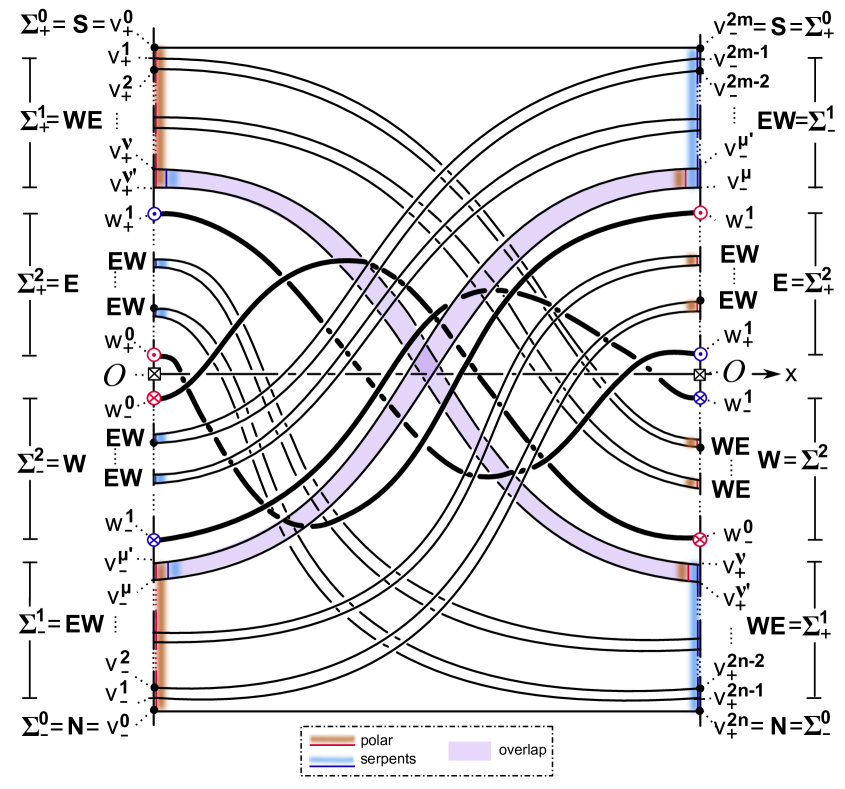
Figure 5.1: An impressionist sketch of the spatial profiles $v(x)$, for all equilibria $v\in\mathcal{E}_{f}$ of a general Sturm 3-meander template. The drawing illustrates the results of proposition 5.3, as well as certain aspects of definition 1.3. For the specific case of a solid octahedron see also fig. 1.1.

Proposition 5.3.

In the above setting and with the notation (4.9) for the equilibrium sets ${\mathcal{E}^{\prime}}_{\pm}^{j}$, the following statements hold true for all $0\leq j\leq 2$ and $\delta=\pm$.

(i) $$v\in{\mathcal{E}^{\prime}}^{j}\quad \Longrightarrow\quad i(v)\leq j$$

(ii) $$v\in\text{clos }{\mathcal{E}^{\prime}}^{j}\quad \Longrightarrow\quad z(v-\mathcal{O})\leq j$$

(iii) $$v\in{\mathcal{E}^{\prime}}_{\pm}^{j}\quad \Longrightarrow\quad z(v-\mathcal{O})=j_{\pm}$$

(iv) $$v_{1},v_{2}\in\text{clos }{\mathcal{E}^{\prime}_{\delta}}^{j}\quad \Longrightarrow\quad z(v_{1}-v_{2})<j\,.$$

Proof..

Claim (iv) is void for $j=0$. For $j=1,2$, claims (i),(iv) have already been proved in proposition 4.3. Claims (i), (iii) for $j=0$ just reiterate $i_{v}=0$ for $v\in\{h_{\iota}^{f}(1),\,h_{\iota}^{f}(N)\}$, by dissipativeness; see (1.25), (1.26), (2.5). Claim (ii) follows from claim (iii), by definition (4.9) of the sets $\text{clos }{\mathcal{E}^{\prime}}^{j}$.

Therefore it only remains to prove claim (iii). Although it is possible to invoke scoops, except for the last nose retraction involving $\mathcal{O}$ itself, we proceed more directly this time. With the abbreviations $\zeta_{j}$:= $z(h_{0}(j)-\mathcal{O})$, for the unsigned zero numbers, and with $s_{j}$:= $\tfrac{1}{2}\text{sign}(\sigma^{-1}(j)-h_{1}^{-1}(\mathcal{O}))$, the explicit recursion (2.5) reads

(5.7) $$\zeta_{j+1}-\zeta_{j}=(-1)^{j+1}(s_{j+1}-s_{j})\,;$$

see also (4.7). Here $1\leq j<k$ and $k=h_{0}^{-1}(\mathcal{O})$ in (2.5). Note that $h_{1}^{-1}(\mathcal{O})=h_{1}^{-1}h_{0}(k)=\sigma^{-1}(k)$. We omit sub- and superscripts $f$ in this proof. We only prove claim (iii) for ${\mathcal{E}^{\prime}_{-}}^{j}$; the cases of ${\mathcal{E}^{\prime}_{+}}^{j}$ are analogous by the trivial equivalence $u\mapsto-u$.

The recursion (5.7) is initialized with

(5.8) $$\zeta_{1}=0\,,\quad s_{1}=-1/2\,,\quad h_{0}(1)<_{0}\mathcal{O}\,,$$

by dissipativeness. This proves claim (iii) for the pole $\mathbf{N}=h_{\iota}(1)$ and settles $j=0$.

We follow the meander path of $h_{0}$ along the $\mathbf{N}$-polar $h_{0}$-serpent

(5.9) $$h_{0}\mathrel{\mathop{\mathchar 58\relax}}\qquad\mathbf{N}\ v_{-}^{1}v_{-}^{2}\ldots v_{-}^{\mu}\ldots v_{-}^{\mu^{\prime}}\ldots$$

up to $v_{-}^{\mu^{\prime}}$, next. By definition 1.3(iii), we have

(5.10) $$\mathbf{N}=h_{0}(1)<_{1}\mathcal{O}<_{1}v_{-}^{1}<_{1}v_{-}^{2}<_{1}\ldots<_{1}v_{-}^{\mu}<_{1}\ldots<_{1}v_{-}^{\mu^{\prime}}$$

along that serpent. See also fig. 1.5. Since $v_{-}^{j}=h_{0}(j+1)$, for $0\leq j\leq\mu^{\prime}$, this implies

(5.11) $$s_{2}=\ldots s_{\mu+1}=\ldots s_{\mu^{\prime}+1}=1/2\,.$$

With recursion (5.7) and initialization (5.8) this proves

(5.12) $$\zeta_{2}=\ldots=\zeta_{\mu+1}=\ldots\zeta_{\mu^{\prime}+1}=1\,.$$

Figure 5.2: The trapping region interior$(\Gamma)$, in a West scoop, and the types of trapped equilibria of a 3-meander template; see the proof of proposition 5.3, (5.14)–(5.16).

By definition 1.3(iv), the $\mathbf{N}$-polar $h_{0}$-serpent is terminated by $w_{-}^{1}$ or $w_{+}^{1}$. In fact $\mathcal{O}\leadsto w_{\pm}^{\iota}$, because $h_{\iota}$-neighbors cannot be blocked. Hence $i(\mathcal{O})=3$ implies $i(w_{\pm}^{\iota})=2$ and, by (2.5),

(5.13) $$z\left(w_{\pm}^{\iota}-\mathcal{O}\right)=2_{\pm}\,.$$

This proves that the $h_{0}$-successor of the serpent termination $v_{-}^{\mu^{\prime}}$ is $w_{-}^{1}$, rather than $w_{+}^{1}$; see fig. 1.5 again. Similarly, the $h_{0}$-predecessor $w_{-}^{0}$ of $\mathcal{O}$ terminates the $\mathbf{N}$-polar $h_{1}$-serpent $v_{+}^{2n}\ldots v_{+}^{\nu}$ along the $h_{1}$-axis. By the Jordan curve property, this traps the meander segment $\mathcal{M}$, from the entry $w_{-}^{1}$ to the exit $w_{-}^{0}$, inside the trapping region defined by the Jordan curve

(5.14) $$\Gamma\mathrel{\mathop{\mathchar 58\relax}}\qquad v_{-}^{\mu^{\prime}}w_{-}^{1}\ \mathcal{O}\ w_{-}^{0}v_{+}^{\nu}\ldots v_{+}^{2}v_{+}^{1}\ \mathbf{S}\,.$$

See fig. 5.2. Here $\Gamma$ consists of $h_{0}$- and $h_{1}$-arcs, alternatingly, and terminates with the part $v_{+}^{\nu}\ldots\mathbf{S}$ of the $\mathbf{S}$-polar $h_{0}$-serpent. The Jordan curve $\Gamma$ is not closed. We consider the remaining part

(5.15) $$v_{-}^{\mu^{\prime}+1}\ldots v_{-}^{2m-1}$$

of the $\mathbf{S}$-polar $h_{1}$-serpent to still be inside the trapping region $\Gamma$ of our meander $\mathcal{M}$ segment from $w_{-}^{1}$ to $w_{-}^{0}$.

Equilibrium vertices $v=h_{0}(j)$ inside $\Gamma$ consist of two types:

(5.16) $$\text{type }1 \mathrel{\mathop{\mathchar 58\relax}}\qquad w_{-}^{0}\leq_{1}v\leq_{1}w_{-}^{1}<_{1}\mathcal{O}\,,\quad\text{and}$$

$$\text{type }2 \mathrel{\mathop{\mathchar 58\relax}}\qquad v\in\{v_{-}^{\mu^{\prime}+1}\ ,\ldots,\,v_{-}^{2m-1}\}>_{1}\mathcal{O}\,.$$

Suppose the meander path $h_{0}$ changes type along the $\mathcal{M}$-arc from $h_{0}(j)$ to $h_{0}(j+1)$. We claim $j$ must be even. Indeed, the trapping region $\Gamma$ ensures that a change of type can only occur via a lower $h_{0}$-arc of the meander $\mathcal{M}$. Therefore the meander must cross the $h_{1}$-axis downward at $v_{j}$:= $h_{0}(j)$, upward at $v_{j+1}=h_{0}(j+1)$, and $j$ must be even.

The types distinguish the signs of $s_{j}$ to be

(5.17) $$s_{j}=\left\{\begin{aligned} &-1/2\quad\text{for}\quad h_{0}(j)\text{ of type }1\,;\\ &+1/2\quad\text{for}\quad h_{0}(j)\text{ of type }2\,.\end{aligned}\right.$$

Indeed the relative ordering of $\sigma^{-1}(j)=h_{1}^{-1}(v_{j})$ and $h_{1}^{-1}(\mathcal{O})$ distinguishes the type of $v_{j}=h_{0}(j)$. In particular, the recursion (5.7) determines the values $\zeta_{j}$ inside the trapping region, with the initialization $\zeta=2$ at $w_{-}^{1}$, to be

(5.18) $$\zeta_{j}=\left\{\begin{aligned} &2\quad\text{for}\quad h_{0}(j)\text{ of type }1\,;\\ &1\quad\text{for}\quad h_{0}(j)\text{ of type }2\,.\end{aligned}\right.$$

Here we have used that $j$ is even at any type change from $v_{j}=h_{0}(j)$ to $v_{j+1}=h_{0}(j+1)$. Hence (5.17) implies a decrease of $\zeta_{j}$ by 1, upon passage from type 1 to type 2, and an increase by 1 upon return. Without change of type, both $s_{j}$ and $\zeta_{j}$ remain unchanged.

By definition (4.9) of ${\mathcal{E}^{\prime}_{\delta}}^{2}$, we see how (5.18) proves claim (iii) for ${\mathcal{E}^{\prime}_{-}}^{2}$. Type 2, together with our previous observation (5.12) proves claim (iii) for ${\mathcal{E}^{\prime}_{-}}^{1}$ and completes the proof of the proposition. ∎

Proof of theorem 5.1..

It is sufficient to establish heteroclinic orbits $\mathcal{O}\leadsto v$ from the unique $i_{\mathcal{O}}=3$ equilibrium to any other equilibrium $\mathcal{O}\neq v\in\mathcal{E}_{f}$. By the Wolfrum lemma 5.2 this is equivalent to showing that

(5.19) $$\mathcal{O},v\ \text{are}\ z(v-\mathcal{O})\text{-adjacent}\,.$$

Note $i_{v}\leq 2$. The relevant information on zero numbers $z$ is listed in proposition 5.3, for the decomposition

(5.20) $$v\ \in\ \mathcal{E}_{f}\smallsetminus\{\mathcal{O}\}\ =\ \bigcup\limits_{j=0,1,2}\left({\mathcal{E}^{\prime}_{-}}^{j}\cup{\mathcal{E}^{\prime}_{+}}^{j}\right)\,;$$

see (4.9), (5.4). Let $v\in{\mathcal{E}^{\prime}_{\delta}}^{j}$, $\delta=\pm$. By proposition 5.3(iii) this is equivalent to $z(v-\mathcal{O})=j_{\delta}$. To show $j$-adjacency of $\mathcal{O},v$, as required by (5.19), we proceed indirectly. Suppose there exists $w\in\mathcal{E}_{f}\smallsetminus\{\mathcal{O},v\}$ such that

(5.21) $$z(w-\mathcal{O})=j_{\delta}=z(v-w)\,;$$

see (5.3). Then the left equality and proposition 5.3(iii) imply $w\in{\mathcal{E}^{\prime}_{\delta}}^{j}$. Hence $v,w$ are both in ${\mathcal{E}^{\prime}_{\delta}}^{j}$, and proposition 5.3(iv) implies

(5.22) $$z(v-w)<j\,.$$

This contradicts the right equality in (5.21), proves (5.19), establishes $\mathcal{O}\leadsto v$, and hence proves theorem 5.1. ∎

6 Signed homeomorphisms for Sturm 3-balls

In this section we prove theorems 2.6 and 2.7. Theorem 2.6 establishes signed homeomorphisms $\Phi^{s}$ between abstract signed 3-cell templates $\mathcal{C}$ and the signed hemisphere decompositions of the Thom-Smale dynamic complex $\mathcal{C}_{f}^{s}$ of the associated Sturm global attractor $\mathcal{A}_{f}$. Theorem 1.2 is the unsigned corollary.

In theorem 2.6 we pass from an abstract signed 3-cell template $\mathcal{C}^{s}$ of cells $c_{v},\ v\in\mathcal{E}$, with a formally prescribed hemisphere decomposition $S_{\pm}^{j}(v)$, to a concrete signed Sturm complex $\mathcal{C}_{f}^{s}$ of unstable manifolds $W^{u}(v),\ v\in\mathcal{E}_{f}$, with hemisphere decomposition $\Sigma_{\pm}^{j}(v)$ such that the signed dynamic complex $\mathcal{C}_{f}^{s}=\mathcal{C}^{s}$ realizes the prescribed signed 3-cell template $\mathcal{C}^{s}$. More precisely, we have to construct a cell preserving homeomorphism

(6.1) $$\Phi^{s}\mathrel{\mathop{\mathchar 58\relax}}\quad\mathcal{C}^{s}\longrightarrow\mathcal{C}_{f}^{s}$$

such that the restrictions define bijections

(6.2) $$\Phi^{s}\mathrel{\mathop{\mathchar 58\relax}} \quad\mathcal{E}\longrightarrow\mathcal{E}_{f}\,;$$

(6.3) $$\Phi^{s}\mathrel{\mathop{\mathchar 58\relax}} \quad c_{v}\longrightarrow W^{u}\left(\Phi^{s}(v)\right)\,;$$

(6.4) $$\Phi^{s}\mathrel{\mathop{\mathchar 58\relax}} \quad S_{\delta}^{j}(v)\longrightarrow\Sigma_{\delta}^{j}\left(\Phi^{s}(v)\right)\,;$$

for all $v\in\mathcal{E}$ and $\delta=\pm$. This is based on the specific construction of the SZS-pair of bijections

(6.5) $$h_{\iota}\mathrel{\mathop{\mathchar 58\relax}}\quad\{1,\ldots,N\}\longrightarrow\mathcal{E}\,,$$

$\iota=0,1$, which is associated to the signed 3-cell template $\mathcal{C}^{s}$ by definition 2.5. As a consequence,

(6.6) $$\sigma\mathrel{\mathop{\mathchar 58\relax}}=h_{0}^{-1}\circ h_{1}$$

is associated to a 3-meander template. See [FiRo16, theorem 5.2]. In theorem 5.1 above we have established that any 3-meander template $\mathcal{M},\sigma$ in fact defines, not just some Sturm attractor but, a Sturm 3-ball $\mathcal{A}_{f}$ via

(6.7) $$\sigma_{f}\mathrel{\mathop{\mathchar 58\relax}}=\sigma\,.$$

In particular $\mathcal{A}_{f}$ comes with boundary orders

(6.8) $$h_{\iota}^{f}\mathrel{\mathop{\mathchar 58\relax}}\quad\{1,\ldots,N\}\longrightarrow\mathcal{E}_{f}$$

of the equilibria $v(x)$ at $x=\iota=0,1$ and defines the Sturm 3-cell template $\mathcal{C}_{f}^{s}$.

Theorem 2.7 then shows, conversely, that any two nonlinearities $f,g$ which satisfy (6.1)–(6.4) for respective signed homeomorphisms $\Phi_{f}^{s},\Phi_{g}^{s}$, possess identical Sturm permutations

(6.9) $$\sigma_{f}=\sigma_{g}\,.$$

In particular their global attractors $\mathcal{A}_{f},\mathcal{A}_{g}$ are $C^{0}$ orbit-equivalent; see [FiRo00]. The homeomorphism

(6.10) $$\Phi_{g}^{s}\circ\left(\Phi_{f}^{s}\right)^{-1}\mathrel{\mathop{\mathchar 58\relax}}\quad\mathcal{C}_{f}^{s}\longrightarrow\mathcal{C}_{g}^{s}$$

can be required to respect decompositions into fast unstable manifolds, as well.

Proof of theorem 2.6..

We establish a signed homeomorphism $\Phi^{s}$: $\mathcal{C}^{s}\rightarrow\mathcal{C}_{f}^{s}$ as in (6.1)–(6.4), by successive extension. Our basic strategy is similar to the planar case discussed in section 3; see in particular the proof of corollary 3.2. As in (3.4) we start from the identical bijections

(6.11) $$\Phi^{s}\mathrel{\mathop{\mathchar 58\relax}}=h_{\iota}^{f}\circ h_{\iota}^{-1}\mathrel{\mathop{\mathchar 58\relax}}\qquad\mathcal{E}\longrightarrow\mathcal{E}_{f}\,,$$

for $\iota=0,1$. Indeed this map does not depend on $\iota$ because $h_{0}^{-1}\circ h_{1}=\sigma=\sigma_{f}=(h_{0}^{f})^{-1}\circ h_{1}^{f}$. This proves claim (6.2). To simplify notation we will use (6.11) to identify barycenter vertices $v\in\mathcal{E}$ of the cells $c_{v}\in\mathcal{C}^{s}$, i.e. intersections of the meander $\mathcal{M}$ of $\sigma$ with the horizontal $h_{1}$-axis, with the equilibria $\Phi^{s}(v)\in\mathcal{E}_{f}$, i.e. with the corresponding intersection of $\mathcal{M}_{f}$ viewed as an equilibrium via the shooting curve of $f$. In particular $\mathcal{E}_{f}=\mathcal{E}$ and

(6.12) $$h_{\iota}^{f}=h_{\iota}\,.$$

In the remaining proof we will first invoke corollary 3.2(i), on planar Sturm attractors, to establish signed homeomorphisms between the two closed hemispheres

(6.13) $$\Phi_{\delta}^{s}\mathrel{\mathop{\mathchar 58\relax}}\qquad\text{clos }S_{\delta}^{2}(\mathcal{O})\longrightarrow\text{clos }\Sigma_{\delta}^{2}(\mathcal{O})\,,$$

for $\delta=\pm$. We will then show how $\Phi_{\pm}^{s}$ can be assumed to coincide on the intersection meridian circle

(6.14) $$S^{1}(\mathcal{O})=\text{clos }S_{+}^{2}(\mathcal{O})\cap\text{clos }S_{-}^{2}(\mathcal{O})\,.$$

In our final step we extend $\Phi_{\pm}^{s}$ to the interior of the unique 3-cell $c_{\mathcal{O}}$.

We have to show how $\Sigma_{-}^{2}(\mathcal{O})=\mathbf{W}_{f}$ and $\Sigma_{+}^{2}(\mathcal{O})=\mathbf{E}_{f}$, in the signed 3-cell template $\mathcal{C}_{f}^{s}$, coincide with the hemispheres $\mathbf{W}$ and $\mathbf{E}$ of the prescribed 3-cell template $\mathcal{C}^{s}$, respectively, via hemisphere homeomorphisms $\Phi_{\pm}^{s}$ as in (6.12). We construct $\Phi_{+}^{s}$ for the closure $\text{clos }\mathbf{E}_{f}=\text{clos }\Sigma_{+}^{2}(\mathcal{O})$ of the eastern hemisphere by a West scoop; the East scoop for $\text{clos }\mathbf{W}_{f}=\text{clos }\Sigma_{-}^{2}(\mathcal{O})$ works analogously. See definition 4.2. The construction of the signed homeomorphism

(6.15) $$\Phi_{+}^{s}\mathrel{\mathop{\mathchar 58\relax}}\qquad\text{clos }\mathbf{E}=\text{clos }S_{+}^{2}(\mathcal{O})\longrightarrow\text{clos }\Sigma_{+}^{2}(\mathcal{O})=\text{clos }\mathbf{E}_{f}$$

for the planar Sturm attractor $\mathcal{A}_{+}$ of the scooped meander $\mathcal{M}_{+},\sigma_{+}$ simply invokes corollary 3.2(i); see (3.14) in particular.

This step requires to show the following claim. Let $(h_{0}^{+},h_{1}^{+})$ be the ZS-pair of the complex

(6.16) $$\mathcal{C}_{+}^{s}\mathrel{\mathop{\mathchar 58\relax}}=\text{clos }\mathbf{E}=\text{clos }S_{+}^{2}(\mathcal{O})\,,$$

viewed as a planar bipolar, and hence signed, complex. Then the West scooped meander permutation $\sigma_{+}$ coincides with the Sturm permutation defined by $h_{\iota}^{+}$:

(6.17) $$\sigma_{+}=\left(h_{0}^{+}\right)^{-1}\circ h_{1}^{+}\,.$$

We will show this claim in lemma 6.1 below.

In lemma 6.2 we will then show how the signed Sturm dynamic complex $\mathcal{A}_{+}=\mathcal{C}_{f_{+}}^{s}$ of $f_{+}$, with $\sigma_{f_{+}}=\sigma_{+}$, coincides with the restriction $(\mathcal{C}_{f}^{s})_{+}$ of the signed Sturm dynamic complex $\mathcal{A}=\mathcal{C}_{f}^{s}$ to the closed hemisphere $\text{clos }\Sigma_{+}^{2}(\mathcal{O})$:

(6.18) $$\mathcal{C}_{f_{+}}^{s}=(\mathcal{C}_{f}^{s})_{+}$$

Combined, (6.16) and (6.18) construct the homeomorphism (6.14) on $\text{clos }\mathbf{E}$.

The construction for $\text{clos }\mathbf{W}$ is analogous, but might differ on the shared boundary meridian $S^{1}(\mathcal{O})$, see (6.13). To remedy this point, let us recall the precise construction of the signed homeomorphisms $\Phi_{\pm}^{s}$ in the planar case. By (3.8) we first extend $\Phi_{\pm}^{s}$ to the 1-skeleta $\mathcal{C}_{\pm}^{1}$ before extending to faces. The faces of $\mathcal{C}_{\pm}^{s}$ are disjoint. On the shared boundary meridian $S^{1}(\mathcal{O})$, it is sufficient to construct $\Phi_{+}^{s}$ and then define $\Phi_{-}^{s}$:= $\Phi_{+}^{s}$, there.

This completes the construction of $\Phi^{s}$ as a signed homeomorphism on the 2-sphere

(6.19) $$\Phi^{s}\mathrel{\mathop{\mathchar 58\relax}}\quad\begin{aligned} S^{2}(\mathcal{O})&=\text{clos }S_{-}^{2}(\mathcal{O})\cup\text{clos }S_{+}^{2}(\mathcal{O})\longrightarrow\\ \longrightarrow\Sigma^{2}(\mathcal{O})&=\text{clos }\Sigma_{-}^{2}(\mathcal{O})\cup\text{clos }\Sigma_{+}^{2}(\mathcal{O})\,.\end{aligned}$$

The radial extension to the respective interiors $c_{\mathcal{O}}\rightarrow W^{u}(\mathcal{O})$ is now obvious and completes the proof of theorem 2.6, up to the next two lemmas 6.1 and 6.2. ∎

Lemma 6.1.

Let $(h_{0}^{+},h_{1}^{+})$ be the ZS-pair of the planar signed complex $\mathcal{C}_{+}^{s}$ defined by the restriction of the 3-cell template $\mathcal{C}^{s}$ to the closed Eastern hemisphere $\text{clos }\mathbf{E}=\text{clos }S_{+}^{2}(\mathcal{O})$. Let $\check{h}_{\iota}$ denote the West scooped paths $h_{\iota}$ of the SZS-pair $(h_{0},h_{1})$ for $\mathcal{C}^{s}$.

Then the paths $h_{\iota}^{+}$ and $\check{h}_{\iota}$ coincide,

(6.20) $$\check{h}_{\iota}=h_{\iota}^{+}\,,$$

for $\iota=0,1$. In particular, consider the Sturm permutation

(6.21) $$\sigma_{*}\mathrel{\mathop{\mathchar 58\relax}}=\left(h_{0}^{+}\right)^{-1}\circ h_{1}^{+}$$

of the planar complex $\mathcal{C}_{+}^{s}$. Then $\sigma_{*}$ coincides with the scooped meander permutation $\sigma_{+}$ of definition 4.2, i.e.

(6.22) $$\sigma_{+}=\sigma_{*}\,,$$

as claimed in (6.17).

The analogous statements hold for the SZ-pair $(h_{0}^{-},h_{1}^{-})$ on $\text{clos }\mathbf{W}=\text{clos }S_{-}^{2}(\mathcal{O})$ and the East scooped paths $\check{h}_{\iota}$.

Proof..

Since the ZS-pair $(h_{0}^{+},h_{1}^{+})$ is unique, we only have to show that the West scooped pair $(\check{h}_{0},\check{h}_{1})$ of definition 4.2, (4.11) forms a ZS-pair in the closed hemisphere $\text{clos }\mathbf{E}$, according to definition 1.1. Let $(h_{0},h_{1})$ denote the original SZS-pair of the 3-cell template $\mathcal{C}^{s}$, prior to the West scoop. By construction, the Hamiltonian paths $h_{\iota}$ form a ZS-pair in $\text{clos }\mathbf{E}$, from their respective first emergence vertex $w_{+}^{\iota}\in\mathbf{E}$ onwards. Before, $h_{0}$ and $h_{1}$ follow the meridians $\mathbf{N}\cup\mathbf{EW}$ and $\mathbf{N}\cup\mathbf{WE}$, respectively, in bipolar order and with interspersed excursions into $\mathbf{W}$. See figs. 1.4 and 2.2. Omitting precisely these Western excursions, in the scooped pair $(\check{h}_{0},\check{h}_{1})$, generates the full $\mathbf{N}$-polar serpents

(6.23) $$\check{h}_{0} \mathrel{\mathop{\mathchar 58\relax}}\qquad\mathbf{N}=v_{-}^{0}v_{-}^{1}\ldots v_{-}^{2m-1}w_{+}^{0}\ldots$$

$$\check{h}_{1} \mathrel{\mathop{\mathchar 58\relax}}\qquad\mathbf{N}=v_{+}^{2n}v_{+}^{2n-1}\ldots v_{+}^{1}w_{+}^{1}\ldots$$

By [FiRo16, lemma 2.7], the $\mathbf{N}$-polar serpents $h_{\iota}^{+}$ of the ZS-pair $(h_{0}^{+},h_{1}^{+})$ in the East hemisphere $\text{clos }\mathbf{E}$ are also full. Hence the scooped paths $\check{h}_{\iota}$ and the ZS paths $h_{\iota}$ coincide everywhere, $\check{h}_{\iota}=h_{\iota}$, as claimed in (6.20). Indeed these paths coincide, both, in their initial $\mathbf{N}$-polar serpent parts before $w_{+}^{\iota}$, and from $w_{+}^{\iota}$ onwards, for $\iota=0,1$. Since $\sigma_{+}=\check{h}_{0}^{-1}\circ\check{h}_{1}$, by definition, (6.20) proves (6.22) and the lemma. ∎

Lemma 6.2.

As claimed in (6.18), the signed Sturm dynamic complex $\mathcal{A}_{+}=\mathcal{C}_{f_{+}}^{s}$ of the West scoop $\sigma_{f_{+}}=\sigma_{+}$ of $\sigma_{f}=\sigma$ coincides with the restriction $(\mathcal{C}_{f}^{s})_{+}$ of the signed Sturm dynamic complex $\mathcal{C}_{f}^{s}$ to the closed Eastern hemisphere $\text{clos }\Sigma_{+}^{s}(\mathcal{O})$.

The analogous statement holds for $\mathcal{A}_{-}=\mathcal{C}_{f_{-}}^{s}$ of the East scoop $\sigma_{f_{-}}=\sigma_{-}$ and the Western restriction $(\mathcal{C}_{f}^{s})_{-}=\text{clos }\Sigma_{-}^{s}(\mathcal{O})$.

Proof..

Consider the Eastern restriction $(\mathcal{C}_{f}^{s})_{+}$ as a given abstract planar signed complex,

(6.24) $$\mathcal{C}_{+}^{s}\mathrel{\mathop{\mathchar 58\relax}}=(\mathcal{C}_{f}^{s})_{+}\,.$$

We then have to show that the planar signed Sturm complex $\mathcal{A}_{+}=\mathcal{A}_{f_{+}}=\mathcal{C}_{f_{+}}^{s}$ of $f_{+}$ with $\sigma_{f_{+}}=\sigma_{+}$ coincides with the abstract planar complex $\mathcal{C}_{+}^{s}$:

(6.25) $$\mathcal{C}_{f_{+}}^{s}=\mathcal{C}_{+}^{2}\,.$$

But in lemma 6.1 we have already observed how the defining scoop paths $(\check{h}_{0},\check{h}_{1})$ of $\sigma_{f_{+}}=\sigma_{+}$ coincide with the ZS-pair $(h_{0}^{+},h_{1}^{+})$ of the prescribed planar complex $\mathcal{C}_{+}^{s}$. Therefore corollary 3.2(i), (3.14) proves claim (6.25) and the lemma. ∎

With the above two lemmas, the proof of theorem 2.6 is now also complete.

Proof of theorem 2.7..

By assumptions (2.31), (2.32) we have a signed homeomorphism $\Phi^{s}$ which identifies the signed versions $\mathcal{C}_{f}^{s},\ \mathcal{C}_{g}^{s}$ of two Sturm 3-ball dynamic complexes $\mathcal{C}_{f},\ \mathcal{C}_{g}$. In short,

(6.26) $$\mathcal{C}_{f}^{s}=\mathcal{C}_{g}^{s}\,.$$

We have to show that the Sturm permutations $\sigma_{f}$ and $\sigma_{g}$ coincide; see (2.33). Moreover, we have to show how $\Phi^{s}$ can be chosen to preserve the fast unstable manifolds; see (2.34).

To show the first claim, $\sigma_{f}=\sigma_{g}$, we only have to show that the boundary orders $h_{\iota}^{f},\ h_{\iota}^{g}$ of the equilibria in $\mathcal{E}_{f},\ \mathcal{E}_{g}$ at $x=\iota=0,1$ coincide. Identifying $\mathcal{E}_{f},\ \mathcal{E}_{g}$ via $\Phi^{s}$, we can write this claim as

(6.27) $$h_{\iota}^{f}=h_{\iota}^{g}\,,$$

for $\iota=0,1$. Indeed (6.27) implies (2.33) by

(6.28) $$\sigma_{f}=(h_{0}^{f})^{-1}\circ h_{1}^{f}=(h_{0}^{g})^{-1}\circ h_{1}^{g}=\sigma_{g}\,.$$

To prove claim (6.27) we invoke proposition 2.3. The signed homeomorphism $\Phi^{s}$: $\mathcal{C}_{f}^{s}\rightarrow\mathcal{C}_{g}^{s}$ identifies the equilibria $\mathcal{E}_{f}$ with $\mathcal{E}_{g}$, and all $\mathcal{E}_{f,\pm}^{j}(v)=\mathcal{E}_{f}\cap\Sigma_{f,\pm}^{j}(v)$ with their counterparts $\mathcal{E}_{g,\pm}^{j}(v)=\mathcal{E}_{g}\cap\Sigma_{g,\pm}^{j}(v)$. In particular, $\Phi^{s}$ identifies all $f$-equilibria $w_{f}(\mathbf{s})$ with their $g$-counterparts $w_{g}(\mathbf{s})$, for identical sign sequences $\mathbf{s}=s_{0}\ldots s_{n-1},\ s_{k}\in\{\pm\}$. By the table of proposition 2.3, this shows that the boundary orders $h_{\iota}^{f},\ h_{\iota}^{g}$ of the respective equilibria coincide, as claimed in (6.27).

We show next how the signed homeomorphism $\Phi^{s}$ can be chosen to respect fast unstable manifolds $W^{j+1}(v)$, as claimed in (2.34). Let $\Phi_{f}^{s}$: $\mathcal{C}^{s}\rightarrow\mathcal{C}_{f}^{s}$ denote the signed homeomorphism which describes $\mathcal{C}_{f}^{s}$ as an abstract 3-cell template $\mathcal{C}^{s}=\mathcal{C}_{f}^{s}=\mathcal{C}_{g}^{s}$. See (6.1). We only have to recall how $\Phi_{f}^{s}$ was constructed by ascending dimensions $i_{v}=i(v)$ of Thom-Smale cells $c_{v}\rightarrow W^{u}(v)$. On the closed ball $\overline{c}_{v}$ with barycenter $v$ we extended $\Phi_{f}^{s}$ radially inwards from the boundary,

(6.29) $$\Phi_{f}^{s}\mathrel{\mathop{\mathchar 58\relax}}\quad\partial c_{v}\longrightarrow\partial W_{f}^{u}(v)=\Sigma_{f}^{i(v)-1}(v)\,.$$

The fast unstable manifolds $W_{f}^{j+1}$, likewise, possess sphere boundaries and, by induction on cell dimension, we may assume

(6.30) $$\Phi_{f}^{s}\mathrel{\mathop{\mathchar 58\relax}}\quad S^{j}(v)\longrightarrow\partial W_{f}^{j+1}(v)=\Sigma_{f}^{j}(v)\,,$$

for $0\leq j<i(v)$. Since $\Phi_{f}^{s}$ is a signed homeomorphism, and passing to the notation of signed hemispheres, we have,

(6.31) $$\Phi_{f}^{s}\mathrel{\mathop{\mathchar 58\relax}}\quad S_{\delta}^{j}(v)\longrightarrow\Sigma_{\delta}^{j}(v)\,,$$

for $\delta=\pm$. The Schoenflies result [FiRo15] provided extensions of (6.31), to the interior balls $B^{j+1}(v)$, such that the standard eigenspaces $E^{j+1}$ mapped to $W_{f}^{j+1}(v)$. Similarly, positive and negative half spaces are mapped to the signed versions of $W_{f}^{j+1}(v)$, separated by $W_{f}^{j}(v)$, for $0\leq j<i(v)$. Replacing radial extensions by this more refined construction of $\Phi_{f}^{s}$ we see how standard (half) eigenspaces just get mapped to (signed) fast unstable manifolds. Since the same statement holds for $\Phi_{g}^{s}$: $\mathcal{C}^{s}\rightarrow\mathcal{C}_{g}^{s}$, on the same 3-cell template complex $\mathcal{C}^{s}$, the combined signed homeomorphism

(6.32) $$\Phi^{s}=\Phi_{g}^{s}\circ\left(\Phi_{f}^{s}\right)^{-1}\mathrel{\mathop{\mathchar 58\relax}}\quad\mathcal{C}_{f}^{s}\longrightarrow\mathcal{C}_{g}^{s}$$

respects signed fast unstable manifolds. This completes the proof of claim (2.34), and the proof of theorem 2.7. ∎

7 Appendix: Wolfrum’s lemma

In this technical appendix we comment on, and repair, a gap in the original proof of Wolfrum’s lemma 5.2.

In [Wo02, theorem 2.1] the lemma has first been formulated in the present form. The gap in the proof arises, formally, by an overinterpretation of realization results in [FiRo99] to provide templates for arbitrary sequences of saddle-node bifurcations. This is not what had been proved there. The relevant result is [FiRo99, lemma 3.1]. Already in the simplest case it is based, first, on a “short arc” nose retraction, via a saddle-node bifurcation. Second, the resulting nose in the meander $\mathcal{M}$ has to be retracted counterclockwise towards the lower, reduced, number of equilibria. See [FiRo99, fig. 3]. This brings the relevant Sturm shooting meanders $\mathcal{M}$ into canonical form, as specified in [FiRo99]. The counterclockwise restriction in the second step has not been addressed in [Wo02].

In fact, the results in [FiRo99] do allow a nose removal by a saddle-node bifurcation which pushes its “short arc” of $\mathcal{M}$ nearly vertically through the horizontal axis. This addresses the first step, locally. Neither before, nor after, such a local sadlle-node bifurcation, however, would the resulting meander be in canonical form, globally.

Therefore it remains crucial to lift the clockwise restriction in the second step, towards canonical meanders. We use the global rigidity of Sturm attractors proved in [FiRo00]: global Sturm attractors $\mathcal{A}_{f}$ and $\mathcal{A}_{g}$ with identical Sturm permutations $\sigma_{f}=\sigma_{g}$ are $C^{0}$ orbit equivalent. In view of that global rigidity, the Sturm permutations on either side of the local saddle-node bifurcation can therefore be realized by shooting curves, again, which are canonical meanders. As a caveat we add that it is still unknown to us whether that second step can be achieved by a global parameter homotopy of Sturm nonlinearities $f$, within the PDE class (1.1). Instead, the rigidity proof in [FiRo00] used a discretization, and subsequent dimensional augmentation, to provide parameter homotopies in the potentially much wider ODE class of finite-dimensional Jacobi systems. At any rate, this remedies both gaps in the proof of [Wo02, theorem 2.1].

The proof of Wolfrum’s lemma is independent of a Conley index argument in [FiRo96] which led to a weaker result. See [Wo02, remark 4.1]. Above we have indicated how arguments of [FiRo99, FiRo00] enter, instead.

References

- [An86] S. Angenent. The Morse-Smale property for a semi-linear parabolic equation. J. Diff. Eqns. 62 (1986), 427–442.
- [An88] S. Angenent. The zero set of a solution of a parabolic equation. J. Reine Angew. Math. 390 (1988), 79–96.
- [Ar88] V.I. Arnold. A branched covering , hyperbolicity and projective topology. Sib. Math. J. 29 (1988) 717–726.
- [ArVi89] V.I. Arnold, M.I. Vishik et al. Some solved and unsolved problems in the theory of differential equations and mathematical physics. Russ. Math. Surv. 44 (1989) 157–171.
- [BaVi92] A.V. Babin and M.I. Vishik. Attractors of Evolution Equations. North Holland, Amsterdam, 1992.
- [BiZh92] J.-M. Bismut and W. Zhang. An extension of a theorem by Cheeger and Müller. With an appendix by François Laudenbach. Astérisque 205, Soc. Math. de France, 1992.
- [Bo88] R. Bott. Morse theory indomitable. Public. Math. I.H.É.S. 68 (1988), 99–114.
- [Br90] P. Brunovský. The attractor of the scalar reaction diffusion equation is a smooth graph. J. Dyn. Diff. Eqns. 2 (1990), 293–323.
- [BrFi86] P. Brunovský and B. Fiedler. Numbers of zeros on invariant manifolds in reaction-diffusion equations. Nonlin.Analysis, TMA 10 (1986), 179–193.
- [BrFi88] P. Brunovský and B. Fiedler. Connecting orbits in scalar reaction diffusion equations. Dynamics Reported 1 (1988), 57–89.
- [BrFi89] P. Brunovský and B. Fiedler. Connecting orbits in scalar reaction diffusion equations II: The complete solution. J. Diff. Eqns. 81 (1989), 106–135.
- [ChVi02] V.V. Chepyzhov and M.I. Vishik. Attractors for Equations of Mathematical Physics. Colloq. AMS, Providence, 2002.
- [Edetal94] A. Eden, C. Foias, B. Nicolaenko, R. Temam. Exponential Attractors for Dissipative Evolution Equations. Wiley, Chichester, 1994.
- [Fi02] B. Fiedler (ed.) Handbook of Dynamical Systems 2, Elsevier, Amsterdam, 2002.
- [FiRo96] B. Fiedler and C. Rocha. Heteroclinic orbits of semilinear parabolic equations. J. Diff. Eqns. 125 (1996), 239–281.
- [FiRo99] B. Fiedler and C. Rocha. Realization of meander permutations by boundary value problems. J. Diff. Eqns. 156 (1999), 282–308.
- [FiRo00] B. Fiedler and C. Rocha. Orbit equivalence of global attractors of semilinear parabolic differential equations. Trans. Amer. Math. Soc. 352 (2000), 257–284.
- [FiRo08] B. Fiedler and C. Rocha. Connectivity and design of planar global attractors of Sturm type, II: Connection graphs. J. Diff. Eqns. 244 (2008), 1255–1286.
- [FiRo09] B. Fiedler and C. Rocha. Connectivity and design of planar global attractors of Sturm type, I: Bipolar orientations and Hamiltonian paths. J. Reine Angew. Math. 635 (2009), 71–96.
- [FiRo10] B. Fiedler and C. Rocha. Connectivity and design of planar global attractors of Sturm type, III: Small and Platonic examples. J. Dyn. Diff. Eqns. 22 (2010), 121–162.
- [FiRo14] B. Fiedler and C. Rocha. Nonlinear Sturm global attractors: unstable manifold decompositions as regular CW-complexes. Discr. Cont. Dyn. Sys. 34 (2014), 5099-5122.
- [FiRo15] B. Fiedler and C. Rocha. Schoenflies spheres as boundaries of bounded unstable manifolds in gradient Sturm systems. J. Dyn. Diff. Eqns. 27 (2015), 597–626.
- [FiRo16] B. Fiedler and C. Rocha. Sturm 3-balls and global attractors 1: Dynamic complexes and meanders. arXiv:1611.02003 [math.DS], 2016.
- [FiRo17] B. Fiedler and C. Rocha. Sturm 3-balls and global attractors 3: Examples. In preparation, 2017.
- [FiSc03] B. Fiedler and A. Scheel. Spatio-temporal dynamics of reaction-diffusion patterns. In Trends in Nonlinear Analysis, M. Kirkilionis et al. (eds.), Springer-Verlag, Berlin 2003, 23–152.
- [Fietal14] B. Fiedler, C. Grotta-Ragazzo and C. Rocha. An explicit Lyapunov function for reflection symmetric parabolic differential equations on the circle. Russ. Math. Surveys. 69 (2014), 419–433.
- [Fr79] J.M. Franks. Morse-Smale flows and homotopy theory. Topology 18 (1979), 199–215.
- [FrPi90] R. Fritsch and R.A. Piccinini. Cellular Structures in Topology. Cambridge University Press, 1990.
- [FuOl88] G. Fusco and W. Oliva. Jacobi matrices and transversality. Proc. Royal Soc. Edinburgh A 109 (1988) 231–243.
- [FuRo91] G. Fusco and C. Rocha. A permutation related to the dynamics of a scalar parabolic PDE. J. Diff. Eqns. 91 (1991), 75–94.
- [Ga04] V.A. Galaktionov. Geometric Sturmian Theory of Nonlinear Parabolic Equations and Applications. Chapman & Hall, Boca Raton, 2004.
- [Ha88] J.K. Hale. Asymptotic Behavior of Dissipative Systems. Math. Surv. 25. AMS, Providence, 1988.
- [Haetal02] J.K. Hale, L.T. Magalhães, and W.M. Oliva. Dynamics in Infinite Dimensions. Springer-Verlag, New York, 2002.
- [He81] D. Henry. Geometric Theory of Semilinear Parabolic Equations. Lect. Notes Math. 804, Springer-Verlag, New York, 1981.
- [He85] D. Henry. Some infinite dimensional Morse-Smale systems defined by parabolic differential equations. J. Diff. Eqns. 59 (1985), 165–205.
- [Hu11] B. Hu. Blow-up Theories for Semilinear Parabolic Equations. Lect. Notes Math. 2018, Springer-Verlag, Berlin, 2011.
- [Jo89] M.S. Jolly. Explicit construction of an inertial manifold for a reaction diffusion equation. J. Diff. Eqns. 78 (1989), 220–261.
- [La91] O.A. Ladyzhenskaya. Attractors for Semigroups and Evolution Equations. Cambridge University Press, 1991.
- [Ma78] H. Matano. Convergence of solutions of one-dimensional semilinear parabolic equations. J. Math. Kyoto Univ. 18 (1978), 221–227.
- [Ma82] H. Matano. Nonincrease of the lap-number of a solution for a one-dimensional semi-linear parabolic equation. J. Fac. Sci. Univ. Tokyo Sec. IA 29 (1982), 401–441.
- [MaNa97] H. Matano and K.-I. Nakamura. The global attractor of semilinear parabolic equations on . Discr. Cont. Dyn. Sys. 3 (1997), 1–24.
- [MP88] J. Mallet-Paret. Morse decompositions for delay-differential equations. J. Diff. Eqns. 72 (1988), 270–315.
- [PaMe82] J. Palis and W. de Melo. Geometric Theory of Dynamical Systems. An Introduction. Springer-Verlag, New York, 1982.
- [PaSm70] J. Palis and S. Smale. Structural stability theorems. Global Analysis. Proc. Simp. in Pure Math. AMS, Providence, 1970.
- [Pa83] A. Pazy. Semigroups of Linear Operators and Applications to Partial Differential Equations. Springer-Verlag, New York, 1983.
- [Ra02] G. Raugel. Global attractors. In [Fi02], 2002, 885–982.
- [Ro91] C. Rocha. Properties of the attractor of a scalar parabolic PDE. J. Dyn. Diff. Eqns. 3 (1991), 575-591.
- [SeYo02] G.R. Sell, Y. You. Dynamics of Evolutionary Equations. Springer-Verlag, New York, 2002.
- [St1836] C. Sturm. Sur une classe d’équations à différences partielles. J. Math. Pure Appl. 1 (1836), 373–444.
- [Ta79] H. Tanabe. Equations of Evolution. Pitman, Boston, 1979.
- [Te88] R. Temam. Infinite-Dimensional Dynamical Systems in Mechanics and Physics. Springer-Verlag, New York, 1988.
- [Wo02] M. Wolfrum. Geometry of heteroclinic cascades in scalar parabolic differential equations. J. Dyn. Diff. Eqns. 14 (2002), 207–241.
- [Ze68] T.I. Zelenyak. Stabilization of solutions of boundary value problems for a second order parabolic equation with one space variable. Diff. Eqns. 4 (1968), 17–22.