Risk-averse model predictive control
Abstract
Risk-averse model predictive control (MPC) offers a control framework that allows one to account for ambiguity in the knowledge of the underlying probability distribution and unifies stochastic and worst-case MPC. In this paper we study risk-averse MPC problems for constrained nonlinear Markovian switching systems using generic cost functions, and derive Lyapunov-type risk-averse stability conditions by leveraging the properties of risk-averse dynamic programming operators. We propose a controller design procedure to design risk-averse stabilizing terminal conditions for constrained nonlinear Markovian switching systems. Lastly, we cast the resulting risk-averse optimal control problem in a favorable form which can be solved efficiently and thus deems risk-averse MPC suitable for applications.
keywords:
Risk measures; Nonlinear Markovian switching systems; Model predictive control.,,,
1 Introduction
1.1 Background and Contributions
There exist two main ways to deal with uncertainty in model predictive control (MPC), namely, the robust and the stochastic approaches. In robust MPC, modeling errors or disturbances are modeled as unknown-but-bounded quantities and the performance index is minimized with respect to the worst-case realization (min-max approach) [18]. However, such worst-case events are unlikely to occur in practice and render robust MPC severely conservative since all statistical information, typically available from past measurements, is ignored.
On the other hand, in stochastic MPC we assume that the underlying uncertainty is a random vector following some probability distribution [14] and minimize the expectation of a performance index; such formulations are significantly less conservative. The driving random process is often taken to be normally and independently identically distributed [12] or it is assumed that it is a finite Markov process [17] and in scenario-based MPC, filtered probability distributions are estimated from data [11]. However, not always can we accurately estimate a distribution from available data, nor does it remain constant in time. Stochastic MPC will guarantee mean-square stability of the closed-loop system only with respect to the nominal probability distribution, therefore, errors in the estimation of that distribution may lead to bad performance or even instability.
The theory of risk measures [26] allows to interpolate between these two extreme cases. Roughly speaking, risk measures quantify the importance and effect of the right tail of a distribution of losses, that is, the impact of the occurrence of extreme events. As such they offer a mathematically elegant tool to tackle problems where we seek to avoid high effect low probability (HELP) events and can be readily used in various applications.
The first steps to risk-averse formulations can be traced back to linear-exponential-quadratic Gaussian control [13] and the study of stochastic control problems under inexact knowledge of the underlying probability distribution which is often termed distributionally robust [10]. Distributionally robust control methodologies have been proposed for linear systems with probabilistic constraints assuming knowledge of some moments of the distribution [27]. The same problem was also recently addressed for Markov decision processes with uncertain transition probabilities [28].
Risk-averse MPC formulations for Markov jump linear systems (MJLS) are studied in [7, 6]. In [6] the authors formulate an MPC optimization problem employing a coherent risk measure of an uncertain cost as an objective function and give conditions under which the MPC control law is stabilizing, albeit for a system with no state-input constraints. This is extended in [7] assuming ellipsoidal state-input constraints. Building up on these results, we further improve on the state of the art by studying nonlinear systems and proposing a computationally favorable formulation for risk-averse optimization problems which leads to low computation times.
In the optimization and operations research communities, the solution of multistage risk-averse optimal control problems has been considered prohibitive as only bundle and cutting-plane methods are currently used [2, 8, 5]. Reported results are limited to short prediction horizons and linear stage cost functions. An alternative solution approach solves the dynamic programming (DP) problem using multiparametric piecewise quadratic programming [16], but its applicability is limited to systems with few states and small prediction horizons [15]. In a 2017 paper, Rockafellar proposed an algorithmic scheme for solving multistage problems using a non-composite (not nested) risk measure recognizing the difficulty of solving problems with nested risk mappings [19]. Indeed, the difficulty lies in that the cost function is written as a series of compositions of typically nonsmooth operators. In Section 5 we present a computationally tractable approach for the solution of multistage risk-averse problems by disentangling this series of compositions. This formulation renders risk-averse MPC suitable for embedded applications.
In this paper we formulate multistage risk-averse optimal control problems using Markov risk measures in a DP setting and derive Lyapunov-type risk-averse stability conditions. We study risk-averse MPC formulations for nonlinear Markovian switching systems under generally nonconvex joint state-input constraints and propose a controller design procedure for nonlinear systems with smooth dynamics and Lipschitz-continuous gradient. Lastly, we provide simulation examples to demonstrate the applicability of the proposed approach.
1.2 Notation
Let be the set of extended-real numbers, the integers in , for let (where the max is taken element-wise). We denote by the vector in with all coordinates equal to . We denote the sets of -by- symmetric positive definite (semidefinite) matrices as (). For two -by- symmetric matrices , means that . We denote the transpose of a matrix by and the identity matrix by . For a , its Jacobian matrix is the mapping defined as , provided that the partial derivatives exist. For we define . For a set , we define its indicator function as if and otherwise. The domain of an extended-real-valued function is . An extended-real-valued function is called proper if its domain is nonempty; it is called lower semi-continuous (lsc) if its lower level sets are closed. An is called level bounded in locally uniformly in if for each and , there is a neighborhood of along with a bounded set such that for all . The effective domain of a set-valued mapping is defined as . For a nonempty set and a finite set we define .
2 Risk-averse optimal control
2.1 Measuring risk
Let be a discrete sample space. A probability measure thereon can be identified by a probability vector with , for . Let be a real-valued random variable on which represents a random cost; for let . The vector identifies the random variable .
The expectation of a random variable with respect to the probability vector is defined as
| (1) |
The notation is to emphasize that the expectation is taken with respect to .
A risk measure on is a mapping . It is called coherent if it satisfies the following properties [26, Sec. 6.3] for , ,
-
A1.
Convexity. ,
-
A2.
Monotonicity. whenever ,
-
A3.
Translation equivariance. ,
-
A4.
Positive homogeneity. .
Trivially, the expectation is a coherent risk measure and so is the essential maximum . A popular risk measure is the average value-at-risk, also known as conditional value-at-risk or expected shortfall, which is defined as
As a result of assumptions A1–A4, coherent risk measures can be written in the following dual form [26, Thm. 6.5]
| (2) |
where is a compact convex set of probability vectors containing which we shall call the ambiguity set of . We may think of a coherent risk measure as the worst-case expectation with respect to a probability distribution taken from a set of probability vectors. We call a polytopic risk measure if is a polytope, i.e., it can be described by for some and . The expectation, the essential maximum and are polytopic risk measures. The ambiguity set of for is the polytope The ambiguity set is the whole probability simplex. Apparently is a polytopic risk measure. interpolates between the risk-neutral expectation operator (, with ) and the worst-case essential maximum ().
2.2 Markovian switching systems
In this work we consider Markovian switching systems
| (3) |
driven by the random parameter which is a time-homogeneous Markov chain with values in a finite set with transition matrix , that is [9]. We call the states of this Markov chain, the modes of (3). We denote the cover of each mode by . We assume that at time we measure the full state and the value of . As the probabilistic information available up to time is fully described by the pair , the control actions may be decided by a causal control law . This formulation aligns with that of the classic textbook [9], but there exist formulations where is not known at time and the control law is a function of only [7].
2.3 Markov risk measures
Consider the space of pairs in equipped with the -algebra and the probability measure . The conditional probability conditioned by the knowledge of can be identified with the probability vector — the -th row of . For a random variable , the conditional expectation of conditioned by , denoted as , is a random variable on , that is , with
| (5) |
We may extend this definition to define conditional variants of risk measures. Following (5), we give the following definition
Definition \thethm (Markov risk measure).
Given a coherent risk measure with ambiguity set and a probability transition matrix of a Markov chain, we define the Markov risk measure as
| (6) |
for all random variables .
This definition falls into the general framework of [21]. This way, with every we associate the coherent risk measure . As with the expectation, the notation is to emphasize that the risk is computed with respect to .
2.4 Risk-averse optimal control and dynamic programming
Consider a stage cost function and a terminal cost . Functions are extended-real-valued, therefore, they can encode constraints such as (4) by taking , . Likewise, can encode constraints on the terminal state of the form by taking , , where contain the origin in their interiors. We may now introduce the following finite-horizon risk-averse optimal control problem
| (7) |
where , for all . As it will become evident in what follows, each one of the infima at stage in (2.4) is parametric in and , that is, the minimization takes place over causal control laws . Note that under assumptions A1 and A2, we may interchange the Markov risk measures with the infima [26, Prop. 6.60] leading to risk-averse multistage formulations discussed in [26, Sec. 6.8.4].
Problem (2.4) can be described by a DP recursion. Inspired by [26, Sec. 6.8], for a we define the DP operator so that
Let be the corresponding set of minimizers for the optimization problem involved in the definition of . This defines the following DP recursion
| (8a) | ||||
| (8b) | ||||
for with , . For with we define the mode-dependent predecessor operator with . Next, we present some fundamental properties of the DP operator .
Proposition \thethm.
We may easily verify the monotonicity property following [4]. An observation that will prove useful in what follows is that if , then . The above risk-averse optimal control problem leads naturally to the statement of a risk-averse MPC problem where control actions are computed by a control law . In Section 3 we state an appropriate risk-based notion of stability and provide conditions on for the MPC-controlled system to be stable.
3 Risk-averse stability
Consider the following Markovian switching system which is controlled by some control law
| (9) |
subject to the constraints . For convenience, we introduce the notation , for . Let denote an admissible path of length of the Markov chain , that is, for . For a given initial state , the solution of (9) at time is denoted as .
In order to be able to define risk-based notions of stability, we must first introduce an appropriate notion of invariance for Markovian switching systems [17].
Definition \thethm (Uniform invariance).
Let be a collection of nonempty closed subsets of and . is called uniformly invariant (UI) for (9) subject to constraints if whenever for all .
For the controlled system (9), the predecessor operator is now defined as . We have that is UI if and only if for all [17].
Given a coherent risk measure and a random variable , let and recursively define , that is [26, Sec. 6.8.2].
We may now give the following stability notion [6].
Definition \thethm (Risk-square exponential stability).
We say that the origin is risk-square exponentially stable (RSES) for system (9) over a set if is UI and for
for all , for some , .
RSES entails that the origin is exponentially mean-square stable for system (9) not only for the nominal probability distribution, but also for those probability distributions in the ambiguity set of the risk measure. In the unconstrained case, RSES corresponds to the notion of uniform global risk-sensitive exponential stability which is defined using the notion of dynamic risk measures [6]. If the underlying risk measure is the expectation operator, then RSES reduces to mean-square exponential stability, whereas, if it is the essential supremum operator, it yields the definition of robust exponential stability. Additionally, since all coherent risk measures are lower bounded by the expectation, RSES is a stronger notion of stability compared to mean-square stability. The following lemma provides Lyapunov-type stability conditions for RSES.
Lemma 1 (RSES conditions).
Suppose there is a , proper, lsc function such that
-
(i)
is a UI set
-
(ii)
, for some for all .
Then, is uniformly bounded in for . If, additionally,
-
(iii)
for all , , for some ,
then, the origin is RSES for system (9) over . {pf} The proof can be found in the appendix.
The uniform boundedness condition in Lemma 1 is reminiscent of the notion of stochastic stability in [9, Sec. 3.3.1]. In fact, if the risk measure in Lemma 1 is the expectation operator, then the uniform boundedness condition is equivalent to mean-square stability [9, Thm. 3.9(6)].
We call a function which satisfies all requirements of Lemma 1, a (mode-dependent) risk-averse Lyapunov function. We may now state conditions on the stage cost and the terminal cost which entail RSES for the risk-averse MPC-controlled system.
4 Risk-averse MPC
4.1 Risk-averse MPC stability
Theorem 2 (RSES of MPC).
Suppose that (i) for some for all , (ii) for some for all , (iii) contain the origin in their interiors (iv) is locally bounded over its domain, that is, for every compact set , there is an so that for all and
| (10) |
Then, the origin is RSES for the risk-averse MPC-controlled system over all compact uniformly invariant subsets of . {pf}The proof can be found in the appendix.
In Thm. 2 we show that is a mode-dependent risk-averse Lyapunov function over compact uniformly invariant subsets of . We shall use this result in the following sections to design risk-averse stabilizing MPC controllers for MJLS as well as nonlinear Markovian switching systems. Note that Condition (iv) in Thm. 2 holds if the following assumption is satisfied (see [18, Prop. 2.15])
Assumption 3 (Local boundedness of ).
For all , functions and are continuous on their domains, and the sets are compact and bounded uniformly in .
4.2 Risk-averse MPC design for MJLS
Here we provide RSES conditions and design guidelines for risk-averse MPC of MJLS [9], that is , using a quadratic stage cost with , and are polytopes with the origin in their interiors. The terminal cost function is taken to be with and . We shall derive conditions on and so that the stabilizing conditions of Thm. 2 are satisfied. Condition is equivalent to
| (11a) | |||
| (11b) | |||
where and the minimization in (11a) is over the space of admissible causal control laws so that . An upper bound to the left hand side of (11a) is obtained by parametrizing We introduce the shorthand notation and , for . Condition (11b) means that is a UI set for the system under the prescribed constraints. Such a set can be determined by the fixed-point iteration with . If this iteration converges in a finite number of iterations — a sufficient condition for which is given in [17, Lem. 21] — to a set , this is a polytopic UI set.
Assuming that is a polytopic Markov risk measure with ambiguity set and using its dual representation, condition (11a) becomes for all and . This condition can be cast as a linear matrix inequality (LMI) by a change of variables , , and :
| (12) |
for all and . The left hand side of (12) is a symmetric matrix, therefore, we show only its upper block triangular part and replaced the lower block triangular part by asterisks () to simplify the notation. Solving this LMI for and yields the linear gains and the cost matrices . LMI (12) has to be solved once offline to determine matrices .
4.3 Risk-averse MPC design for nonlinear Markovian switching systems
For nonlinear systems, an obvious choice for the terminal cost function would be — meaning, for — but that would lead to a very conservative design. Here we exploit the system linearization at the origin to determine a terminal cost function and terminal constraints which render the MPC-controlled system RSES. We shall first draw the following assumption for the nonlinear dynamics:
Assumption 4.
For each , is differentiable with -Lipschitz Jacobian.
We use a parametric controller of the form and define the associated closed-loop function , . Function can be written as a composition of with the linear mapping , therefore, its Jacobian matrix will be Lipschitz-continuous with Lipschitz constant which is bounded above by
| (13) |
The linearization of the nonlinear system at the origin is an MJLS with and given by the Jacobian matrices, with respect to and respectively, of at the origin. That is, , . For notational convenience, we define the following quantities
The objective is to design the terminal cost and terminal constraints for the risk-averse MPC problem using to yield an LMI. While our design will be based on the linearized dynamics, we need to account for the linearization error. To this end, we shall derive a quadratic upper bound for in a neighborhood of the origin.
Theorem 5.
Suppose that Assumptions 3 and 4 hold and
| (14) |
for , , , and satisfy the requirements of Thm. 2 with for some for all ,
| (15) |
and . If is a UI set for (9), then the origin is RSES for the MPC-controlled system over the compact UI subsets of .
The proof can be found in the appendix.
According to Thm. 5, one first needs to select for each such that (14) holds true. In the most common case where and are quadratic functions, this is precisely an LMI of the form (12) with in place of solving which we obtain matrices and and determine the constants and find so that (15) holds. The last step is to determine a UI set for the nonlinear system . We may cast the nonlinear system as a linear one with bounded additive disturbance — indeed, as we show in the proof of Thm. 5, . We may follow the approach of [25] in order to determine a polytopic robustly invariant set.
5 Computationally tractable formulation of risk-averse optimal control problems
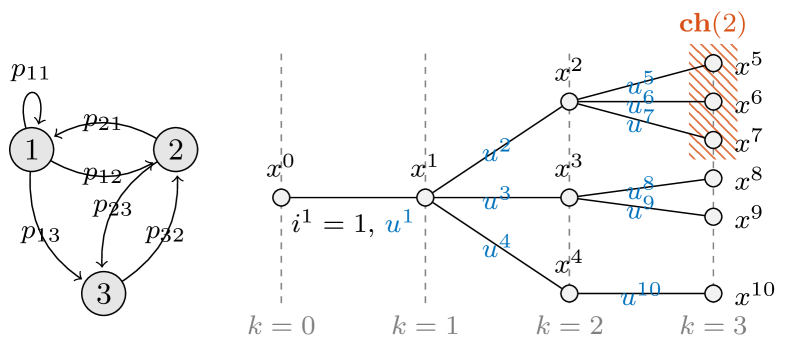
Starting from an initial state and initial mode and computing control actions according to a causal control law , the future states of the Markovian system, up to some future time , span a scenario tree — a tree-like structure such as the one shown in Fig. 1. Note that the state at a node , the input and mode leading to that node are denoted as , and respectively.
The possible realizations of the system state at time define the nodes of the tree. The set of all nodes at stage defines the set . The set of nodes in which are reachable from a node is called the set of children of and is denoted by which is a subset of . The space becomes a probability space with for . As illustrated in Fig. 1, the system dynamics on the scenario tree is described by , for and , .
On the scenario tree, we define a process as follows: for we define . Moreover, . When the underlying risk measure is polytopic with with , then
where in the first equation we interchanged with using [3, Prop. 2.6.4] using the fact that the level sets of the mapping are bounded because is compact. The last equality is because of LP duality. Traversing indices from back to , we define , which boils down to
for . This formulation allows us to deconvolve the nested Markov risk measures. Indeed, is the optimal value of the following minimization problem
Note that this formulation does not require the enumeration of the vertices of which, for instance, in the case of increases exponentially with the number of modes. The above optimization problem is solved at every time instant with , being the current state and mode of the system. Solving this problem yields the optimal control actions at each node of the scenario tree. The first value, , defines the risk-averse MPC controller . Note that in the particular case of an MJLS where stage-wise and terminal costs are quadratic and the constraints are polyhedral and/or ellipsoidal, we obtain a quadratically constrained quadratic program (QCQP) which can be solved very efficiently online as we show in Section 6. The above reformulation can be applied to risk measures whose ambiguity set is described by a set of conic inequalities (using conic duality) such as the entropic value-at-risk [1].
6 Illustrative example
Here we demonstrate the design of stabilizing risk-averse MPC controllers for a nonlinear system. We consider the following nonlinear Markovian switching system with three modes:
| (16) |
The system matrices are
and parameters , , . Stage-wise cost matrices are and for The nominal and actual transition matrices are given by
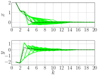
The nonlinear system is constrained to be inside the box for all three modes. Using we compute the controller design parameters of Thm. 5 which are shown in Table 1. We take the terminal sets to be ellipsoidal . Finally, we simulate the system for different values of parameter of after we formulate the problem as described in Section 2.4, with initial condition and . Resulting system trajectories are reported in Fig. 2. The proposed methodology successfully stabilizes the nonlinear system in the presence of uncertainty in the Markov transition matrix.
| 1 | 0.4421 | 0.2407 | 0.1783 | 0.1563 |
|---|---|---|---|---|
| 2 | 0.2210 | 0.3775 | 0.4121 | 0.3556 |
| 3 | 0.6631 | 0.1668 | 0.1130 | 0.0973 |
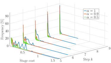
A similar effect is observed when inspecting the distribution of for three MPC controllers. MPC controllers with higher (closer to stochastic MPC) allow for higher costs, albeit with low probability. On the other hand, the risk-averse controller with (closer to minimax MPC) tends to produce cost distributions with shorter right tails. Interestingly, the point is not feasible for the worst case controller (). The cost distributions are shown in Fig. 3.

7 Conclusions
We proposed a control methodology for constrained nonlinear Markovian switching systems. The proposed stability analysis framework hinges on dynamic programming and leads to the formulation of risk-based Lyapunov-type conditions. These conditions can be translated into an LMI when the dynamics is linear, while, when the system is nonlinear a design methodology was proposed. In the case of MJLS, the resulting optimization problem can be formulated as a QCQP and can be solved efficiently online enabling its use in embedded applications.
We believe that risk-averse problems possess a favorable structure which can be further exploited to lead to parallelizable implementations akin to ones already developed for stochastic optimal control problems [24, 23, 22]. We plan to investigate risk-constrained formulations where we impose acceptable risk of violating the constraints instead of hard state/input constraints. This has a potential to make the overall design much less conservative.
This work was supported by the EU-funded H2020 project DISIRE, grant agreement No. 636834, the KU Leuven Research Council under BOF/STG-15-043, the Ford-KU Leuven Research Alliance under project No. KUL0023 and by Research Foundation Flanders, FWO, under project No. G086318N.
References
- [1] A. Ahmadi-Javid. Entropic value-at-risk: A new coherent risk measure. J. Optimiz. Theory App., 155(3):1105–1123, 2012.
- [2] T. Asamov and A. Ruszczyński. Time-con-sistent approximations of risk-averse multistage stochastic optimization problems. Math. Prog., 153(2):459–493, 2015.
- [3] D. Bertsekas, A. Nedić, and A. Ozdaglar. Convex analysis and optimization. Athena Scientific, 2003.
- [4] D.P. Bertsekas. Dynamic Programming and Optimal Control, volume II. Athena Scientific, 4th edition, 2012.
- [5] S. Bruno, S. Ahmed, A. Shapiro, and S. Stree. Risk neutral and risk averse approaches to multistage renewable investment planning under uncertainty. Eur. J. Oper. Res., 250(3):979 – 989, 2016.
- [6] Y.-L. Chow and M. Pavone. A framework for time-consistent, risk-averse model predictive control: Theory and algorithms. In ACC, pages 4204 – 4211, Portland, USA, 2014.
- [7] Y.-L. Chow, S. Singh, A. Majumdar, and M. Pavone. A framework for time-consistent, risk-averse model predictive control: Theory and algorithms. arXiv preprint arXiv:1703.01029v1, 2017.
- [8] R.A. Collado, D. Papp, and A. Ruszczyński. Scenario decomposition of risk-averse multistage stochastic programming problems. Ann. Oper. Res., 200:147–170, 2012.
- [9] O.L.V. Costa, M.D. Fragoso, and R.P. Marques. Discrete-time Markov Jump Linear Systems. Springer, 2005.
- [10] J. Goh and M. Sim. Distributionally robust optimization and its tractable approximations. Oper. Res., 58(4-part-1):902–917, Aug 2010.
- [11] C.A. Hans, P. Sopasakis, A. Bemporad, J. Raisch, and C. Reincke-Collon. Scenario-based model predictive operation control of islanded microgrids. In IEEE CDC, Osaka, Japan, Dec 2015.
- [12] P. Hokayem, E. Cinquemani, D. Chatterjee, F. Ramponi, and J. Lygeros. Stochastic receding horizon control with output feedback and bounded controls. Automatica, 48(1):77–88, 2012.
- [13] D.H. Jacobson. Optimal stochastic linear systems with exponential performance criteria and their relation to deterministic differential games. IEEE Trans. Aut. Control, 18(2):124–131, 1973.
- [14] A. Mesbah. Stochastic model predictive control: An overview and perspectives for future research. IEEE CSM, 36(6):30–44, Dec 2016.
- [15] P. Patrinos and H. Sarimveis. An explicit optimal control approach for mean-risk dynamic portfolio allocation. In ECC, pages 3364–3370, Jul 2007.
- [16] P. Patrinos and H. Sarimveis. Convex parametric piecewise quadratic optimization: theory and algorithms. Automatica, 47(8):1770–1777, 2011.
- [17] P. Patrinos, P. Sopasakis, H. Sarimveis, and A. Bemporad. Stochastic model predictive control for constrained discrete-time Markovian switching systems. Automatica, 50(10):2504–2514, Oct 2014.
- [18] J.B. Rawlings and D.Q. Mayne. Model Predictive Control: Theory and Design. Nob Hill Publishing, Madison, 2009.
- [19] R.T. Rockafellar. Solving stochastic programming problems with risk measures by progressive hedging. Set-Valued and Variational Analysis, Jul 2017.
- [20] R.T. Rockafellar and Roger J.-B. Wets. Variational analysis, volume 317. Springer, 2011.
- [21] A. Ruszczyński. Risk-averse dynamic programming for Markov decision processes. Math. Progr., 125(2):235–261, Oct 2010.
- [22] A.K. Sampathirao, P. Sopasakis, A. Bemporad, and P. Patrinos. Distributed solution of stochastic optimal control problems on GPUs. In IEEE CDC, Osaka, Japan, Dec 2015.
- [23] A.K. Sampathirao, P. Sopasakis, A. Bemporad, and P. Patrinos. Proximal quasi-Newton methods for scenario-based stochastic optimal control. In IFAC WC, 2017.
- [24] A.K. Sampathirao, P. Sopasakis, A. Bemporad, and P. Patrinos. GPU-accelerated stochastic predictive control of drinking water networks. IEEE TCST, 26(2), 2018.
- [25] R.M. Schaich and M. Cannon. Robust positively invariant sets for state dependent and scaled disturbances. In IEEE CDC, pages 7560–7565, Dec 2015.
- [26] A. Shapiro, D. Dentcheva, and Ruszczyński. Lectures on stochastic programming: modeling and theory. SIAM, 2014.
- [27] B.P. Van Parys, D. Kuhn, P.J. Goulart, and M. Morari. Distributionally robust control of constrained stochastic systems. IEEE TAC, 61(2):430–442, 2016.
- [28] P. Yu and H. Xu. Distributionally robust counterpart in Markov decision processes. IEEE TAC, 61(9):2538–2543, 2016.
Appendix A Appendix
Proof of Lemma 1. Define and, for fixed let . We have
| (17) |
where the inequality is because of the subadditivity of (A1 and A4) and the last equality is because is independent of . In light of Cond. (ii) and given that and because of (A) and property A2 we have that . Using properties A3 and A4, which proves the first part of Lemma 1.
By Cond. (ii), for some , so with . We have and , so . Then, and recursively
| (18) |
By the left hand side of Cond. (iii), and applying and using (18) and, subsequently the right hand side of Cond. (iii), .
Proof of Theorem 2. Let be a compact UI set. By (8), Then, for ,
The first inequality is because and property A2. We have that for all . Because of Cond. (iii), we may find such that , for . By Cond. (iv), there is an . Then, for all , . Because of Cond. (i) and the definition of , we have that for all for . The proof is complete since satisfies all conditions of Lemma 1.