Spectroscopic signatures of different symmetries of the superconducting order parameter in metal-decorated graphene

Abstract

Motivated by the recent experiments indicating superconductivity in metal-decorated graphene sheets, we investigate their quasi-particle structure within the framework of an effective tight-binding Hamiltonian augmented by appropriate BCS-like pairing terms for p-type order parameter. The normal state band structure of graphene is modified not only through interaction with adsorbed metal atoms, but also due to the folding of bands at Brillouin zone boundaries resulting from a $\sqrt{3}\times\sqrt{3}R30^{\circ}$ reconstruction. Several different types of pairing symmetries are analyzed utilizing Nambu-Gorkov Green’s function techniques to show that $p+ip$-symmetric nearest-neighbor pairing yields the most enhanced superconducting gap. The character of the order parameter depends on the nature of the atomic orbitals involved in the pairing process and exhibits interesting angular and radial asymmetries. Finally, we suggest a method to distinguish between singlet and triplet type superconductivity in the presence of magnetic substitutional impurities using scanning tunneling spectroscopy.

Keywords: metal decorated graphene, superconductivity, electronic structure, spectroscopy

1 Introduction

Since its discovery, graphene has fascinated the scientific community with its remarkable electronic properties, such as high electron mobility and the anomalous quantum Hall effect. [1, 2, 3] Although pristine graphene seems to lack superconductivity (SC), it can be induced via the proximity effect[4]. More notably, SC state has been found in intercalated graphite structures, especially CaC₆, where metal atoms reside in the space between the loosely interacting graphene layers [5, 6, 7, 8, 9, 10]. Intriguingly, from the point of view of their electronic structure, intercalated graphite structures have also provided a promising platform for developing high capacity rechargeable batteries [11]. The findings of SC in these materials have motivated recent experiments, which indicate that metal decoration might also induce SC in a single graphene sheet [9, 8], although the nature of SC remains unclear.

An early theoretical study of metal-decorated graphene by Uchoa and Castro Neto [12] considered various pairing symmetries in the presence of band folding effects of a $\sqrt{3}\times\sqrt{3}R30^{\circ}$ reconstruction. That study discusses electron-phonon and electron-plasmon mediated SC, and suggests that the extended s-wave or p+ip -wave pairing with nearest neighbor matrix elements is more feasible than s-wave pairing with onsite matrix elements. Although Ref. [12] emphasizes the electron-plasmon mechanism, the possibility of phonon mediated SC has attracted attention in intercalated graphene [10] where ab initio electron-phonon coupling computations rule out multigap SC, but support anisotropic pairing between electrons [13].

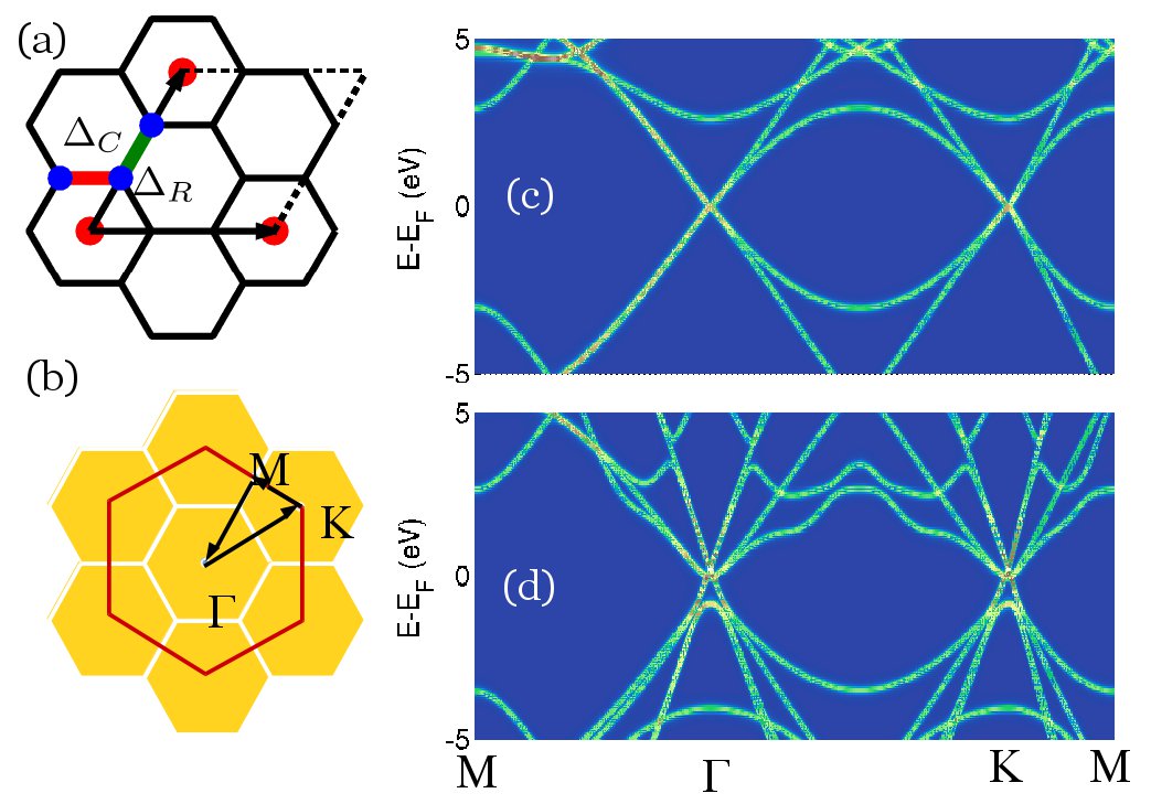
Figure 1: (Color online) (a) Geometry of the $\sqrt{3}\times\sqrt{3}R30^{\circ}$ structure of CaC${}_{6}.$ The primitive cell is indicated as a parallellepiped. The range and direction of the anomalous Hamiltonian matrix elements $\Delta_{R}$ and $\Delta_{C}$ are indicated as green and red lines between nearest neighbor sites, respectively. (b) Reciprocal space of the $\sqrt{3}\times\sqrt{3}R30^{\circ}$ structure, along with the first Brillouin zone of pristine graphene (red hexagon). (c) Folded band structure of pristine graphene along high symmetry directions marked in (b). (d) Folded band structure of metal-decorated graphene.

The purpose of this study is to examine spectroscopic signatures of different symmetries of the superconducting order parameter (OP) in metal-decorated graphene. We take CaC₆ as an exemplar system, and focus on the quasiparticle (QP) and scanning tunneling spectra (STS) associated with specific OPs. We do not attempt to assess the nature of the mechanism mediating pairing, but rather seek to unfold the fingerprints of different symmetries of OPs in QP dispersions and the related local densities of states. While the emphasis is on variations of $s$- and $p+ip$-symmetric singlet superconductivity, we also distinguish between singlet- and triplet-type pairing by introducing a magnetic impurity into the system. Our analysis is carried out within the framework of an effective tight-binding (TB) Hamiltonian, which we augment with appropriate pairing matrix elements to model various OPs. The Hamiltonian is fitted to DFT calculations in order to correctly capture the low-energy states and their orbital characters. The realistic gap widths are of the order of $6-11meV$ (see, e.g., [5]), but we exaggerate the amplitudes of the anomalous terms in order to highlight pairing effects on the electronic structure. This allows us to focus on the behavior of the salient consequences of different superconducting order parameters.

2 Methodology

Our model Hamiltonian involves one $s$-orbital and three $p$-orbitals for each atom. The electron, hole and spin degrees of freedom are incorporated as follows:

$$\hat{H}=\sum_{\alpha\beta\sigma}(\varepsilon_{\alpha}c^{\dagger}_{\alpha\sigma}c_{\alpha\sigma}+V_{\alpha\beta}c^{\dagger}_{\alpha\sigma}c_{\beta\sigma})+\hat{H}_{\textrm{SC}}+\hat{H}_{\textrm{MAG}}.$$ (1)

Here $c^{\dagger}_{\alpha\sigma}$ ($c_{\alpha\sigma}$) is the real-space creation (annihilation) operator, $\alpha$ is a composite index which encodes both the site and orbital information, and $\sigma$ is the spin index. The on-site orbital energy ($\varepsilon_{\alpha}$) and the hopping integral between orbitals $\alpha$ and $\beta$ ($V_{\alpha\beta}$) are obtained within the Slater-Koster formalism [14, 15]. All parameters in the normal state part of the TB Hamiltonian are fitted to the low-energy DFT band structure of CaC₆ obtained using the Quantum Espresso [16, 17] package. Fig. 1(a) and 1(b) depict the real space structure of the system indicating the structures for pristine honeycomb lattice and the lattice with the reduced symmetry. Fig. 1(c) Shows the folded band structure for the pristine graphene and, for comparison, 1(d) shows the effect of Ca decoration. A more detailed analysis of the band structure is given in Appendix A.

For the SC part of the Hamiltonian, $\hat{H}_{SC}$, different OPs (anomalous matrix elements of the Hamiltonian) $\Delta_{\alpha\sigma\beta\sigma^{\prime}}(\lambda)$ are modeled through the choices of atomic orbitals, spin degrees of freedom, and the pairing symmetries (labeled $\lambda$, see also Appendix B). However, in all cases, we have artificially enhanced the amplitudes of OP matrix elements to better identify and highlight the gaps in QP dispersions and local densities of states (LDOSs). Thus, we write the SC part of the Hamiltonian as

$$\hat{H}_{SC}=\sum_{\alpha\beta\sigma}(\Delta_{\alpha\sigma\beta\sigma^{\prime}}(\lambda)c^{\dagger}_{\alpha\sigma}c^{\dagger}_{\beta-\sigma}+\Delta_{\beta\sigma^{\prime}\alpha\sigma}^{\dagger}(\lambda)c_{\beta-\sigma}c_{\alpha\sigma}).$$ (2)

It is important to distinguish between the symmetry of the order parameter $\lambda$ and the character of the involved atomic orbitals $\alpha$ and $\beta$. For example, if the matrix element $\Delta_{\alpha\beta}(\lambda)$ has $p+ip$-symmetry, its complex phase is the same as the phase of $x_{\alpha\beta}+iy_{\alpha\beta}$, where $x$ and $y$ refer to the relative coordinates of the atoms with orbitals $\alpha$ and $\beta.$ To put it simple, we mainly use the symmetry choices of Ref. [12] where, in addition to spherically symmetric onsite matrix elements of s-wave order parameter, there are also nearest neighbour matrix elements which can expanded to follow $\propto k_{x}+ik_{y}$ (see also Refs. [18, 19]). The main novelty here is that in Ref. [12] the basis consists of $p_{z}$ orbitals of carbon, but in our cases the basis is significantly larger (See also appendices A and C).

We will find that the QP-dispersion of SC singlet and triplet pairings are indistinguishable unless a spin-dependent perturbation is present. With this in mind, we allow the possibility of introducing a substitutional magnetic impurity into the Hamiltonian (1) via the term

$$\hat{H}_{MAG}=Um_{\gamma}(c^{\dagger}_{\gamma\uparrow}c_{\gamma\uparrow}-c^{\dagger}_{\gamma\downarrow}c_{\gamma\downarrow}).$$ (3)

Here $\gamma$ refers to the index of the orbital contributing to local magnetic moment. The impurity is modeled by replacing one metal atom with a model atom (see Fig. 4(a) insert), where the two spin states are split via differences in their on-site energies. In order to create a visible effect, we have taken $Um_{\gamma}=\pm 1.0eV$ for the spin-up and spin-down $p$-orbitals of the impurity atom, respectively.

We analyze the electronic structure generated by the Hamiltonian by utilizing Bogoliubov-de Gennes equations and the associated tensor (Nambu-Gorkov) Green’s function ${\cal G}$[20, 21]:

$${\cal G}={\cal G}^{0}+{\cal G}\mathbb{\cal D}{\cal G}^{0},$$ (4)

where ${\cal G}^{0}$ is the Nambu-Gorkov Green’s function without electron-hole interaction,

$${\cal G}=\left(\begin{array}[]{cc}G_{e}&F\\ F^{\dagger}&G_{h}\end{array}\right)~{}\textrm{with}~{}{\boldmath c}_{\alpha}=\left(\begin{array}[]{c}c_{\alpha\uparrow}\\ c_{\alpha\downarrow}\\ c^{\dagger}_{\alpha\uparrow}\\ c^{\dagger}_{\alpha\downarrow}\end{array}\right)$$

and

$$\mathbb{\cal D}=\left(\begin{array}[]{cc}0&\tau\\ \tau^{\dagger}&0\end{array}\right)$$

Here, $G_{e}$ and $G_{h}$ denote the spin-resolved Green’s functions for electrons and holes, respectively, and the matrix elements of the operator $\tau$ represent the interaction terms of the Hamiltonian of Eq. 1. As in Refs. [22, 23], the elements of Nambu-Gorkov Green’s function provide us the local density of states

$$\rho_{\alpha\sigma,\beta\sigma^{\prime}}=-\frac{1}{2\pi i}\left(\cal G^{+}_{\alpha\sigma,\beta\sigma^{\prime}}-\cal G^{-}_{\beta\sigma^{\prime},\alpha\sigma}\right)$$ (5)

and the electron-hole pairing amplitude is

$$\rho_{eh}=\textrm{Tr}(FF^{\dagger}).$$ (6)

The preceding equations allow us to obtain contributions to various quantities from different orbitals, as well as from the electron, hole, or spin degrees of freedom. The foremost use of the density matrix is different presentations of energy states as a function of different degrees of freedom. For example the QP dispersion can be expressed as $\rho(E,k)$-diagram, which is essentially the band diagram. Furthermore, one can take a trace of $\rho(E,k)$ over the electron part of the basis as is done in most of the QP dispersions presented in this work, or to consider the anomalous electron-hole terms as in Fig. 3. (c-f) (see also Ref. [23]).

Another use of the density matrix is simulations of scanning tunneling microscopy/spectroscopy (STM/STS), where we apply the Todorov-Pendry approach [24] (see also Ref. [25]) in which the differential conductance $\sigma$ between orbitals of the tip ($t,t^{\prime}$) and the sample ($s,s^{\prime}$) is given by[26, 23]

$$\sigma=\frac{dI}{dV}=\frac{2\pi e^{2}}{\hbar}\sum_{tt^{\prime}ss^{\prime}}\rho_{tt^{\prime}}(E_{F})V_{t^{\prime}s}\rho_{ss^{\prime}}(E_{F}+eV)V_{s^{\prime}t}^{\dagger}.$$ (7)

We will see that structural variations in the SC gap do not lead to variations in the LDOS, which are pronounced enough to allow identification of the underlying coupling mechanism via regular dI/dV-spectroscopy. We consider therefore the effect of a local magnetic impurity to determine how this perturbation will be seen in STM/STS under various pairing symmetries. In addition to the regular STM topographic maps, we compute current polarization maps in constant current mode where the regular dI/dV spectrum is scaled by the normal state spectrum and the polarized differential conductance spectrum, Here, current polarization, following Ref. [27], is defined as:

$$P_{I}=\frac{I_{\uparrow}-I_{\downarrow}}{I_{\uparrow}+I_{\downarrow}}$$ (8)

where current can be obtained with numerical integration of equation 7. Still following [27], the differential conductance polarization is

$$P_{\sigma}=\frac{\frac{dI}{dV}_{\uparrow}-\frac{dI}{dV}_{\downarrow}}{\frac{dI}{dV}_{\uparrow}+\frac{dI}{dV}_{\downarrow}}.$$ (9)

Note that these expressions refer to the case where components of spin are perpendicular to the sample surface, although practical spin-resolved STM often involves filtering components parallel to the surface [27, 28]. The modeling of the more complicated case of spin-filtering in the presence of horizontal spin components will be considered elsewhere.

3 Results

The following discussion will emphasize three main points: (1) Since the singlet p+ip-wave symmetry of the OP $\Delta(\lambda)$ seems to be the most effective route toward forming the SC gap, we will focus on different orbital combinations for creating a p+ip-wave OP. (2) Concerning the normal-state band structure, the metal atoms lead to a Kekulé-type folding [29, 30] of the $\pi^{*}$-band with a gap and, in addition, new conical non-folded bands appear due to rehybridization of the p-orbitals of carbon and metal atoms, see Appendix A for details. To determine how these folded and conical bands contribute to SC and the OP, we consider OP matrix elements between the relevant atomic orbitals in two scenarios: (a) Use $p_{z}$ orbitals of neighboring carbon atoms to construct $\pi$-type OP or (b) use horizontal p-orbitals of carbon to construct $\sigma$- or $\pi$-type OP. In this connection, we discuss the possibility of non-equivalent $\Delta_{R}$ (radial) and $\Delta_{C}$ (angular) terms. (3) Finally, although we focus on singlet $p+ip$ superconductivity, we consider the possibility to experimentally distinguish between singlet and triplet cases in the presence of magnetic impurity.

3.1 SC state: $\sigma$ vs. $\pi$-type order parameter

We start by considering the effect on SC of different types of OPs with $p_{x}+ip_{y}$ symmetry in terms of contributing atomic orbitals. As the first case, we scrutinize Hamiltonian matrix elements $\Delta_{\alpha\beta}(\lambda)$, where $\alpha$ and $\beta$ are the $p_{z}$ orbitals of the two neighboring carbon atoms. This can be characterized as p-type coupling with a $\pi$-type orbital-orbital character. Such a matrix element opens up a gap with coherence peaks for the $\pi^{*}$ bands under electron or hole doping, see Fig. 2(a), which is similar to the observations in intercalated bulk CaC₆ in Ref. [7]. Since these matrix elements directly couple only with the $p_{z}(C)$-orbitals, they have little effect on the conical bands and, as a result, they remain essentially intact.

These interlayer bands (IL) (see Appendix A) with a Dirac point mainly involve $p_{x/y}$(C) character, and therefore, we must also consider the p-wave matrix elements $\Delta_{\alpha\beta}(\lambda)$, where $\alpha$ and $\beta$ are linear combinations of the $p_{x}$ and $p_{y}$ orbitals of two neighbouring carbon atoms. There are two possibilities: the orbitals can be combined to make a $\sigma$-type combination, where the hybridized p-orbitals point along the bond between the two carbon atoms or a $\pi$-type combination, where the orbital is oriented in the perpendicular direction. Both these $\pi$ and $\sigma$-type matrix elements open up an SC gap uniformly at $\Gamma$ when the Fermi-energy lies outside the gap of the folded $\pi^{*}$ band, see Fig. 2(b); when $E_{F}$ lies within the gap, the SC gap opens only due to the $\sigma$- but not the $\pi$-type matrix element. This directional dependence is likely dependent on the hybridization of the horizontal $p$-orbitals with $p_{z}$(C)-orbitals, which contribute to the conical bands only within the gap of the $\pi^{*}$ band (See discussion of orbital contributions in Appendix A).

The distinction between the two kinds of orbital contributions can also be seen in Fig. 2(c), where an inspection of the $p_{z}$(C) contribution to the partial density of states (PDOS) shows the presence of a clear SC gap. If the horizontal p-orbital contribution is taken into account as well, the PDOS projected onto $p_{x/y}$(C) also shows an SC gap (see Fig. 2(d)), but the intensity is an order of magnitude smaller.

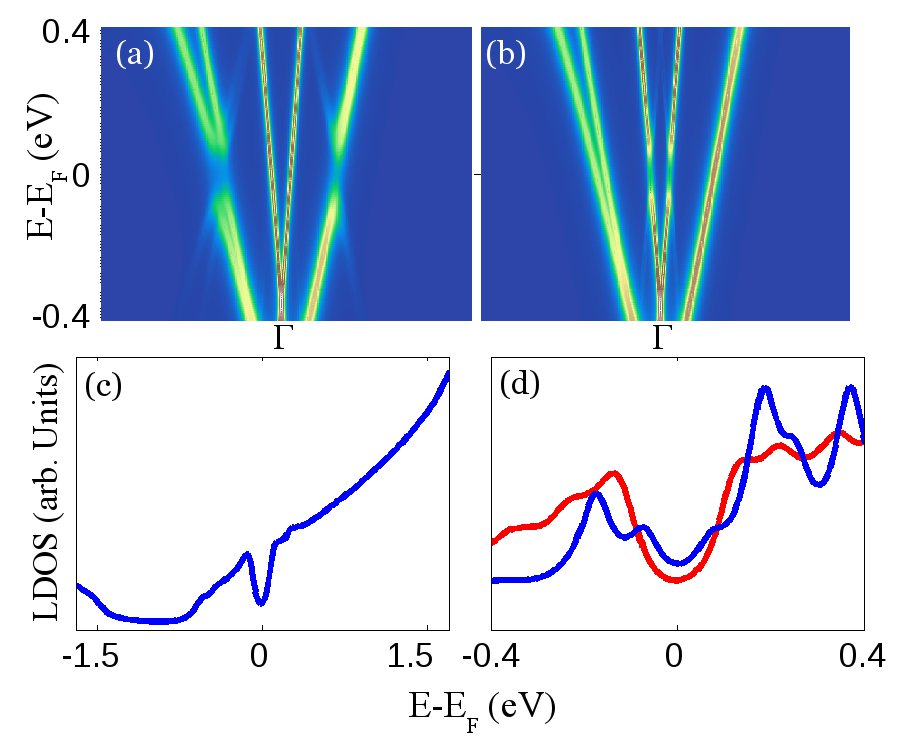
Figure 2: (Color online) QP dispersion for electron doped CaC₆ when the matrix elements of $\Delta$ are between (a) $p_{z}$-orbitals and (b) $p_{x/y}$-orbitals of neighbouring C atoms. (c) Contribution from $p_{z}$(C) to the density of states corresponding to the parabolic bands in (a). (d) PDOS from p_z(C) (red) and p_x(C)+p_y(C) in the region near $E_{F}$ (blue line is multiplied by a factor of 10).

3.2 Anisotropy of order parameter $\Delta$: radial vs. angular bonds

In constructing SC matrix elements, it is useful to make a distinction between the radial bonds [$\Delta_{R}$, Fig. 1(a)], which connect the two carbon atoms between the neighboring metal atoms, and what may be called angular bonds [$\Delta_{C}$, Fig. 1(a)], which connect phenyl-ring-like hexagons around the metal atoms.

Our calculations indicate that the angular matrix element, $\Delta_{C}$, contributes strongly to gap formation, see Figs. 3 (a) and (b), and that the radial matrix element alone is not sufficient for opening an SC gap in the electronic spectrum. The E-k-dispersion in Fig. 3 further indicates that the anomalous amplitudes $|F|^{2}$ lead to some QP-hybridization via both types of matrix elements, but the angular symmetry plays a dominant role. Interestingly, however, there is little difference between the amplitudes of the resulting outgoing radial and angular matrix elements of the anomalous Green’s function, $|F_{C}|^{2}$ and $|F_{R}|^{2}.$ Since the OP $\Delta$ would be coupled self-consistently with $F$ [20, 21], the directional homogeneity of the anomalous Green’s function would indicate connections between the symmetry of the OP and the bosonic mechanism underlying SC. In particular, a directionally anisotropic OP can only be obtained if the related bosonic modes are directionally anisotropic.

3.3 STM/STS and pairing mechanism in the presence of a magnetic impurity: singlet vs. triplet pairing

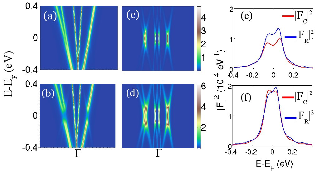
Figure 3: (Color online) QP dispersion for electron doped CaC₆ when only (a) the radial and (b) the angular matrix elements of $\Delta$ are included for all $p$-orbitals. (c) and (d) Energy-momentum dispersion of electron-hole pairing amplitudes corresponding to (a) and (b), respectively. (e) and (f) Matrix elements $|F_{R}|^{2}$ (blue curves) and $|F_{C}|^{2}$ (red curves) of electron-hole pairing amplitudes, where (e) and (f) correspond to (a) and (b), respectively.

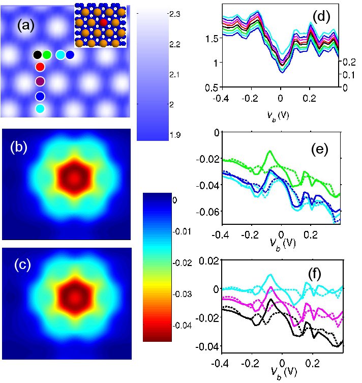
Figure 4: (Color online) (a) Simulated STM topographic map for CaC₆ in the presence of a magnetic impurity. Colored dots indicate the real space positions where the corresponding computed STS spectra are shown in (d). The inset shows the simulated primitive cell with C (blue) and Ca (yellow) atoms along with the impurity atom (red). (b) and (c) Spin-polarized topographic map for the system in (a) for singlet- and triplet-type pairing, respectively. (d) dI/dV spectra for the SC state scaled by the normal state spectra at positions indicated in (a). Lines with various colors correspond to tip positions given by the dots of the same color in (a). All spectra have been scaled by the corresponding normal state spectra. (e) Spin-polarized dI/dV-spectra computed at three different points along the horizontal line joining the impurity atom in the inset in (a) with Ca. Results for singlet pairing (solid lines) and triplet pairing (dashed lines) are shown. (f) Spin-polarized dI/dV-spectra computed at three different points along the vertical line joining the two Ca atoms. Results for singlet pairing (solid lines) and triplet pairing (dashed lines)

are shown.

As noted already, we expect little difference between the STS/STM spectra of CaC₆ for singlet and triplet pairing. However, since a singlet Cooper pair has total spin $S=0$, and triplet has $S=1$, a difference could be induced via a magnetic perturbation. Accordingly, we consider the effects of substituting a Ca atom with a magnetic impurity. Note that the STM corrugation map of Fig 4(a) shows the metal atoms as bright spheres, and gives no hint of the magnetic perturbation. Similarly, scaled dI/dV spectra in Fig. 4(d) computed at various positions (see colored dots in Fig. 4(a)) show little variation with position. Qualitatively, the same kind of scaled set of spectra are obtained for both the singlet and the triplet case. We thus adduce that a regular STM/STS measurement will not detect the presence of a magnetic impurity.

Fig. 4(b) shows that when we consider a map of polarized current, $P_{I}$-map (Eq. 8), the magnetic impurity at the center of the figure is clearly detected, with the perturbation extending essentially only to the neighboring Ca atoms. The polarization is seen to be the strongest on the six carbon atoms surrounding the impurity, being nearly as strong as it is on the impurity atom. A hexagonal pattern of slightly lower (ferromagnetic) polarization is seen in the neighborhood of the six Ca atoms with the magnetic effect rapidly dying out as we move further away from the impurity. Note that this map is practically identical for both singlet- and triplet-case (Fig. 4(b) and (c)). This indicates that the $P_{I}$-map also cannot be used to distinguish between singlet and triplet pairing, even though this map clearly shows the magnetic perturbation.

Figures 4(e) and (f) finally consider polarized differential conductance, $P_{\sigma}$, see Eq. (9). The spectra are now seen to distinguish between singlet (solid lines) and triplet (dashed line) pairing around the magnetic impurity. For the singlet case, polarization changes abruptly around the coherence peaks and varies roughly linearly in the gap region. In sharp contrast, in the triplet case, we see a minimum at the coherence peak energies, and a maximum at energies between these peaks. These fingerprints of singlet and triplet pairing should be observable in spin-polarized dI/dV-spectra, and allow thus a handle on the underlying pairing mechanism.

4 Summary and Conclusions

We consider p+ip -wave singlet superconductivity in metal-decorated graphene within the framework of a tight-binding Hamiltonian based on first-principles normal state band structure, and discuss the characteristic spectroscopic fingerprints of different superconducting order parameters.

Both the in-plane $p_{x/y}$(C)-orbitals and the out-of-the-plane $p_{z}$(C)-orbitals are needed to open up a superconducting gap. Anomalous matrix elements between the $p_{z}$-orbitals open a gap between the $\pi^{*}$-bands whereas matrix elements between the $p_{x/y}$-orbitals are required to open the gap in the conical interlayer bands. Therefore, ARPES experiments with sufficiently high resolution could distinguish between superconducting gaps in different bands, and could thus be used to identify the atomic orbitals involved in the underlying pairing mechanism. On the other hand, although a few meV gap expected in intercalated graphite [5] could be observed via STM/STS experiments as indicated by the results of Fig. 2(c), one would not be able to distinguish between different pairing symmetries from the measured spectra.

Due to the Kekulé structure induced by metal decoration, the order parameter is anisotropic. As a result, the superconducting gap forms mainly due to the angular matrix elements, which reflect the couplings between the neighboring carbons circling a metal atom. Unfortunately, there is no direct way to experimentally detect directional anisotropy in the order parameter. One could speculate about the possibility of obtaining the anomalous QP spectrum through a measurement using a superconducting STM tip, where the directional anisotropy might be reflected in the quasiparticle interference (QPI) patterns.

Our analysis shows that the character of the SC gap depends on the nature of the atomic orbitals at the Fermi energy involved in the pairing process, which drive interesting angular and radial asymmetries in the SC order parameter. The computed STM/STS spectra with and without a magnetic impurity indicate that a magnetic impurity will essentially be invisible in a standard (spin-unresolved) spectrum. This, however, is not the case in a spin-resolved STM/STS spectrum, where the polarization around the impurity can be seen clearly, and singlet vs. triplet pairing can be distinguished in the polarized differential conductance spectrum of Eq. 9. Our study indicates that spin-polarized measurements would provide new insight into the nature of the order parameter and its symmetry in metal-decorated graphene systems. An interesting prospect is, if superconductivity of graphene could be tuned with modulations in metal decoration. Based on the calculated effects of magnetic impurity, as well as the dependence of the order parameter on the folded bands vs. decoration induced conical band, we suggest STM/STS experiments on metal decoration with magnetic and non-magnetic substitutional impurities.

Acknowledgments This work benefited from the resources of Institute of Advanced Computing, Tampere. T.S. is grateful to Väisälä Foundation for financial support. The work at Northeastern University was supported by the US Department of Energy (DOE), Office of Science, Basic Energy Sciences grant number DE-FG02-07ER46352 (core research), and benefited from Northeastern University’s Advanced Scientific Computation Center (ASCC), the NERSC supercomputing center through DOE grant number DE-AC02-05CH11231, and support (applications to layered materials) from the DOE EFRC: Center for the Computational Design of Functional Layered Materials (CCDM) under DE-SC0012575. Conversations with Esa Räsänen and Sami Paavilainen are gratefully acknowledged.

Appendix A Geometric and electronic structure and normal state band characters

Figs. 1(a) and (b) show how the $\sqrt{3}\times\sqrt{3}R30^{\circ}$ reconstruction reduces lattice symmetry. As a result, bands fold at the two inequivalent $K$-points of the large BZ of pristine graphene to the $\Gamma$-point of the small BZ of the metal-decorated graphene sheet. The new lattice of C atoms can also be viewed as a Kekulé-distorted graphene lattice (see Refs. [29, 30]). This distortion opens a gap at the Dirac point of the $\pi^{*}$-type bands, which is clearly seen in the band structures of Fig. 1(c) and (d). As is well known [12, 10, 6], in addition to the $\pi^{*}$-bands, “hourglass”-like bands are formed from the $sp^{2}$-hybridized horizontal $p$-orbitals of C atoms and orbitals of the metal atoms. We refer to these two types of bands as $\pi^{*}$- and interlayer-bands (IL-bands). This nomenclature, however, is not followed consistently in the literature, and for this reason, we comment further on this point.

Since the gapped or Kekulé-distorted bands are doubly degenerate (in addition to spin degeneracy), they are folded from the graphene $K$-points. The LDOS decomposition in Fig. 5 shows that these bands possess a strong p_z(C)-character especially in the vicinity of the gap; the Ca orbitals mix with these bands at higher energies. The conical IL-band, on the other hand, merely possesses the spin-degeneracy and it is, therefore, a genuine decoration-induced feature at the $\Gamma$-point. An analysis of the wavefunction shows that IL-band is dominated by p_x/y(C) orbitals, which originate from $sp^{2}$-hybridization. Since orbitals of Ca atoms overlap weakly with the horizontal p(C)-orbitals, Kekulé-distortion does not open a gap in these bands.

Figure 5: (Color online) Contribution of various orbitals in the band structure of Fig. 1(d) for decorated CaC₆: (a) Horizontal p-orbitals of C; (b) Folded $\pi^{*}$ orbitals of C; (c) Horizontal $p$-orbitals of Ca; (d) $p_{z}$-orbitals of Ca.

Appendix B Implementation of singlet and triplet superconductivity in the tight binding Hamiltonian

Here we consider anomalous matrix elements of the Hamiltonian in using the basis set: $(|\alpha\uparrow\rangle,|\beta\uparrow\rangle,|\alpha\downarrow\rangle,|\beta\downarrow\rangle).$ For a singlet configuration ($s=0$), antisymmetric two-particle states with $m_{s}=0$ are of the form $|\alpha\uparrow\beta\downarrow\rangle-|\alpha\downarrow\beta\uparrow\rangle.$ For a triplet ($s=1$), the state is symmetric with respect to spin flip, and hence $|\alpha\uparrow\beta\downarrow\rangle+|\alpha\downarrow\beta\uparrow\rangle$ corresponds to $m_{s}=1$, whereas $|\alpha\uparrow\beta\uparrow\rangle$ and $|\alpha\downarrow\beta\downarrow\rangle$ stands for cases $m_{s}=1$ and $-1$, respectively. Construction of the order parameters then follow the derivation given in Refs. [33, 34] for topological superconductors.

In constructing the order parameters, we assume that the combined angular momentum is $J=0$, which couples orbital and spin quantum numbers as: $m_{l}+m_{s}=0$, i.e., $m_{l}=-m_{s}.$ For the singlet state we need an s-wave order parameter $\Delta(s)$ and a sub-Hamiltonian for the four orbitals given by:

$$\left(\begin{array}[]{cccc}0&0&0&\Delta(s)\\ 0&0&\Delta(s)&0\\ 0&-\Delta(s)&0&0\\ -\Delta(s)&0&0&0\end{array}\right)$$

since spin-flip changes the sign of the matrix element.

In addition to the symmetry with respect to the orbital/spin permutations, one must also account for the directional dependence of the order parameter $\Delta.$ Define $x_{\alpha\beta}=x_{\alpha}-x_{\beta}$, and likewise for the other coordinates, the form apart from an amplitude prefactor is as follows [$\Delta(s)$ is just a complex number (totally symmetric)]:

$$\Delta(z)\propto\frac{z_{\alpha\beta}}{r_{\alpha\beta}}=\cos{(\theta_{\alpha\beta})}$$

and

$$\Delta(\pm)\propto\frac{(x_{\alpha\beta}\pm iy_{\alpha\beta})}{r_{\alpha\beta}}=\sin{(\theta_{\alpha\beta})}e^{(\pm i\varphi_{\alpha\beta})}.$$

Hence, this scaling takes into account the dimensionality of the system by introducing the appropriate rotational angles.

In the triplet case, we need a spatially antisymmetric wave function, i.e., we need p-symmetric matrix elements. If we first look at the case $m_{s}=0$, we need a $p_{z}$-symmetric matrix element $\Delta(z).$ Since switching the order of the orbitals in the two-particle state changes the sign, the sub-Hamiltonian goes into the form:

$$\left(\begin{array}[]{cccc}0&0&0&\Delta(z)\\ 0&0&-\Delta(z)&0\\ 0&\Delta(z)&0&0\\ -\Delta(z)&0&0&0\end{array}\right).$$

For $m_{s}=\pm 1$, the symmetry of the matrix element is $p_{\mp}=p_{x}\mp ip_{y}.$ Following the anticommutation arguments for matrix elements $\Delta(\mp)$, we end up with the following sub-Hamiltonian:

$$\left(\begin{array}[]{cccc}0&\Delta(-)&0&0\\ -\Delta(-)&0&0&0\\ 0&0&0&\Delta(+)\\ 0&0&-\Delta(+)&0\\ \end{array}\right).$$

Hence, these matrix elements consist of up-up and down-down terms. Finally, the total electron-hole block will be:

$$\left(\begin{array}[]{cccc}0&\Delta(-)&0&\Delta(s)+\Delta(z)\\ -\Delta(-)&0&\Delta(s)-\Delta(z)&0\\ 0&-\Delta(s)+\Delta(z)&0&\Delta(+)\\ -\Delta(s)-\Delta(z)&0&-\Delta(+)&0\\ \end{array}\right).$$

Appendix C Parametrization of the Hamiltonian.

We utilize the Slater-Koster tables [14, 15] to determine the distance and directional dependence of the Hamiltonian matrix elements, but their amplitudes are fitted to QE calculated band structures especially at low energies. The amplitudes for the matrix elements and the onsite terms are as follows:

Table 1: Amplitudes of the Slater-Koster terms.

overlap	amplitude
$ss\sigma$	-0.80
$sp\sigma$	0.24
$pp\sigma$	3.24
$pp\pi$	-0.81

Table 2: Onsites and cut-off lenghts.

$\varepsilon_{s}(C)$	$\varepsilon_{p}(C)$	$\varepsilon_{s}(Ca)$	$\varepsilon_{p}(Ca)$	$r_{C-C}$	$r_{Ca-Ca}$	$r_{C-Ca}$
$-13.6eV$	$-0.610eV$	$6.89$	$7.39eV$	$1.48\AA$	$4.30\AA$	$2.52\AA$

References

References

- [1] A. H. Castro Neto, F. Guinea, N. M. R. Peres, K. S. Novoselov, and A. K. Geim Rev. Mod. Phys. 81, 109(2009).
- [2] L. Banszerus, M. Schmitz, S. Engels, J. Dauber, M. Oellers, F. Haupt, K. Watanabe, T. Taniguchi, B. Beschoten and C. Stampfer, Sci. Adv. 1, 6 (2015).
- [3] P. M. Ostrovsky, I. V. Gornyi, and A. D. Mirlin, Phys. Rev. B 77, 195430 (2008).
- [4] H.B. Heersche et al., Nature (London) 446, 56 (2007).
- [5] T. E. Weller, M. Ellerby, S. S. Saxena, R. P. Smith and N. T. Skipper, Nature Physics 1, 39 - 41 (2005).
- [6] S.-L. Yang et al, Nature Comm 5, 3493 (2014).
- [7] N. Bergeal, V. Dubost, Y. Noat, W. Sacks, D. Roditchev, N. Emery, C. Herold, J-F. Mareche, P. Lagrange, and G. Loupias, Phys. Rev. Lett. 97, 077003 (2006).
- [8] J. Chapman et al., Scientific Reports, 6, 23254(2016).
- [9] B. M. Ludbrook et al, PNAS 112, 38 (2015).
- [10] G. Profeta et al, Nature Physics 8, 131-134 (2012).
- [11] E. J. Yoo, J. Kim, E. Hosono, H.-S Zhou, T. Kudo and I. Honma, Nano Lett., 8,2277-2282 (2008).
- [12] B. Uchoa, and A. H. Castro Neto, Phys. Rev. Lett. 98, 146801(2007).
- [13] A. Sanna, G. Profeta, A. Floris, A. Marini, E. K. U. Gross, and S. Massidda Phys. Rev. B 75, 020511(R) (2007).
- [14] J. C. Slater and G. F. Koster, Simplified LCAO method for the periodic potential problem. Phys. Rev. 94, 1498 (1954).
- [15] W.A. Harrison, Electronic Structure and the properties of solids - The Physics of The Chemical Bond, (Dover Publications, New York, 1989).
- [16] P. Giannozzi, S. Baroni, N. Bonini, M. Calandra, R. Car, C. Cavazzoni, D. Ceresoli, G. L. Chiarotti, M. Cococcioni, I. Dabo, A. Dal Corso, S. Fabris, G. Fratesi, S. de Gironcoli, R. Gebauer, U. Gerstmann, C. Gougoussis, A. Kokalj, M. Lazzeri, L. Martin-Samos, N. Marzari, F. Mauri, R. Mazzarello, S. Paolini, A. Pasquarello, L. Paulatto, C. Sbraccia, S. Scandolo, G. Sclauzero, A. P. Seitsonen, A. Smogunov, P. Umari, R. M. Wentzcovitch, J.Phys.:Condens.Matter 21, 395502 (2009), http://arxiv.org/abs/0906.2569
- [17] We used the pseudopotentials C.pbe-rrjkus.UPF and Ca.pz-n-vbc.UPF from http://www.quantum-espresso.org.
- [18] Jacob Linder,Annica M. Black-Schaffer, Takehito Yokoyama, Sebastian Doniach, and Asle Sudbo, Phys. Rev. B90, 80, 094522 (2009).
- [19] Annica M. Black-Schaffer and Sebastian Doniach Phys. Rev. B 75, 134512 (2007).
- [20] A.A. Abrikosov, L.P.Gorkov, and I.E. Dzyaloshinski. Methods of Quantum Field Theory in Statistical Physics. Dover, New York, 1975.
- [21] A.L. Fetter and J.D. Walecka, Quantum Theory of Many-Particle Systems. Dover (2003).
- [22] M. Paulsson and M. Brandbyge Phys. Rev. B 76, 115117(2007).
- [23] J. Nieminen, I. Suominen, R.S. Markiewicz, H. Lin, and A. Bansil, Phys. Rev. B80, 134509 (2009).
- [24] T.N. Todorov, G.A.D. Briggs and A.P. Sutton, J.Phys.: Condens. Matter 5, 2389 (1993); J.B. Pendry, A.B. Prêtre and B.C.H. Krutzen, ibid., 3, 4313 (1991).
- [25] J. Tersoff and D.R. Hamann, Phys. Rev. B 31, 805 (1985).
- [26] J. Nieminen, H. Lin, R.S. Markiewicz, and A. Bansil, Phys. Rev. Lett. 102, 037001 (2009).
- [27] D. Wortmann, S. Heinze, Ph. Kurz, G. Bihlmayer, and S. Blügel, Phys. Rev. Lett 86, 4132(2001).
- [28] R Wiesendanger Reviews of Modern Physics 81 (4), 1495(2009).
- [29] Gomes, K. K., Mar, W., Ko, W., Guinea, F. & Manoharan, H. C. Designer Dirac fermions and topological phases in molecular graphene. Nature 483, 306310 (2012).
- [30] Paavilainen, S. Ropo, M, Nieminen, J., Akola, J., Räsänen, E. Coexisting Honeycomb and Kagome Characteristics in the Electronic Band Structure of Molecular Graphene. Nano Letters, 16, 3519-3523(2016).
- [31] C. Chamon, Phys. Rev. B 62, 2806 (2000).
- [32] F. Reinert and S. Hüfner, Photoemission Spectroscopy with Very High Energy Resolution: Studying the Influence of Electronic Correlations on the Millielectronvolt Scale, edited by S. Hüfner (Springer, 2007).
- [33] Xiao-Liang Qi and Shou-Cheng Zhang Rev. Mod. Phys. 83, 1057 (2011).
- [34] Topological Insulators and Topological Superconductors, B. A. Bernevig and T. L. Hughes, Princeton University Press, Princeton, 2013.