Abstract

In conformal quantum mechanics with the vacuum of a real scaling dimension and with a complete orthonormal set of energy eigenstates which is preferable under the unitary evolution, the dilatation expectation value between energy eigenstates monotonically decreases along the flow from the UV to the IR. In such conformal quantum mechanics there exist bounds on scaling dimensions of the physical states and the gauge operators.

1 Introduction

A space-time symmetry is of great importance in defining theories to describe the laws of nature. By reconciling quantum mechanics with the Poincaré symmetry group, one obtains relativistic quantum field theory in which fields are classified by the Casimir operators of the Poincaré group as quantum numbers, i.e. the spin and the mass. In conformal field theory, operators are classified by the Casimir operators of the conformal group. Since the mass cannot be invariant under the conformal group as it is a dimensional parameter, it is replaced by the scaling dimension. The main subject in the study of conformal field theory is the operators which have a definite spin and scaling dimension. By virtue of symmetry properties of the correlation functions, even if we have no Lagrangian description, we can study conformal field theory from consistency conditions, via the conformal bootstrap method [1, 2, 3], which leads to a certain spectrum of the allowed scaling dimensions of the theory.

In this work we investigate conformal quantum mechanics, which is obtained by the incorporation of the $SL(2,\mathbb{R})$ conformal symmetry of time into quantum mechanics. In conformal quantum mechanics, the Casimir operators of the conformal group $SL(2,\mathbb{R})$ is just associated with the scaling dimensions. The important fact is that while in the analysis of the spectrum for conformal field theory the dilatation is identified with the Hamiltonian in the radial quantization, in conformal quantum mechanics they should be distinguished. Therefore conformal quantum mechanics would be a theoretically appropriate playground to study the relationship between the energy and the scaling dimension.

Here we aim to address two main issues in conformal quantum mechanics that admits the vacuum and the primary operators by examining its correlation functions.

The first question is the irreversibility of the RG flow in quantum mechanical system. The RG transformation is associated to the scaling process from the UV to the IR. The information in the UV of the theory is expected to be lost in the IR since correlation functions in field theory are valid only at scales smaller than the cutoff by integrating out higher momentum degrees of freedom. Zamolodchikov’s $c$-theorem [4] proves the irreversibility of the RG flow in two dimensional field theories by establishing the existence of a $c$-function, a function of coupling constant and energy scale that decreases along the RG flow and is stationary at the RG fixed points, where its value equals the crucial parameter in the theory, i.e. central charge. For even $d$-dimensional conformal field theory (CFT_d), Cardy [5] proposes a $c$-function as the quantity appearing in the trace anomaly given by the one point function of the trace of the energy momentum tensor on the sphere; $c\sim\langle T^{\mu}_{\mu}\rangle_{S^{d}}$. There have been various proposals in higher dimensional extensions of a $c$-function; $d=3$ [6, 7, 8], $d=4$ [9] and $d=6$ [10, 11]. An exploration of a $c$-function in conformal quantum mechanics is attractive since it may provide a direct explanation of the irreversibility as the theory distinguishes the energy and the scaling dimension. We observe that the trace part of the energy momentum tensor is related to the conserved current of the dilatation $D$ and we show that the expectation value of the dilatation between preferable energy eigenstates under the unitary evolution, which we will call a $D$-function $D(E)\sim\langle E|D|E\rangle$ possesses similar properties as a $c$-function.

In the second part, we present a pair of simple no-go theorems. In relativistic quantum field theory, interaction of massless particles with spins is highly constrained due to the Lorentz symmetry. For higher spin massless particles the negative energy state and negative probability occur. Even though they are mathematically well-defined, they would not appear in experimental results. The Weinberg-Witten theorem [12] claims that a theory with the Lorentzian covariant conserved current $J^{\mu}$ does not admit the spin $s>\frac{1}{2}$ massless charged particles and that a theory with the Lorentzian covariant energy momentum tensor $T^{\mu\nu}$ does not involve spin $s>1$ massless particles. The theorem is proven by investigating the matrix elements of the charge operators between one massless particle states of spin and momenta. In this work we apply a similar method to matrix elements in conformal quantum mechanics. We derive new types of the no-go theorems which impose constraints on scaling dimensions of the physical states constructed in terms of the primary operators and the preferred vacua under the unitary evolution as $-\frac{1}{2}\leq d+\Delta\leq\frac{1}{2}$. This admits the free bosonic scalar with $d+\Delta=-\frac{1}{2}$, the free fermion with $d+\Delta=0$ and the bosonic auxiliary field with $d+\Delta=\frac{1}{2}$. We also find a bound on scaling dimension of the gauge operators which may couple to physical states with the scaling dimensions $d+\Delta$ as $0<\delta_{Q}\leq 2$. While bosonic scalar of $d+\Delta=-\frac{1}{2}$ may couple to the gauge fields of $\delta_{Q}=2$, the fermion of $d+\Delta=0$ can interact with those of $\delta_{Q}=1$.

The organization of this paper is as follows. In section 2 we review the $SL(2,\mathbb{R})$ conformal symmetry of time. In section 3 we discuss the vacuum state $|\Omega\rangle$ which can be labeled by the scaling dimension $d$. It characterizes the theory under consideration. In section 4 we study the energy eigenstate $|E\rangle$ and introduce the $D$-function as the dilatation expectation value between the energy eigenstates. We see that the $D$-function behaves as a $c$-function. In section 5 we derive the no-go theorems. They provide bounds on scaling dimensions of the vacuum, of the primary operator and of the gauge operator as well as constraints. In section 6 we conclude with some open questions and future directions.

2 Conformal Symmetry of Time

In general a conformal group is the group of space-time transformations that preserve angles locally between two distinct points, whose definition contains a metric tensor. Such definition does not seem to be suitable for one-dimension since there are neither angle nor metric tensor. In addition, if we follow the definition, we find a diffeomorphism group $\mathrm{Diff}(\mathbb{R})$, which requires a gravity coupling. It does not seem realistic to consider the quantum mechanical system which is invariant under the $\mathrm{Diff}(\mathbb{R})$, that is the topological quantum mechanics. In this work we are interested in the conformal symmetry transformation of time which consists of the translation, the scaling transformation and the conformal boost. The corresponding generators are the Hamiltonian $H=i\partial_{t}$, the dilatation $D=it\partial_{t}$ and the special conformal transformation $K=it^{2}\partial_{t}$ respectively. Let

$$G =uH+vD+wK$$ (2.1)

be a linear combination of the three generators where $u$, $v$, $w\in\mathbb{C}$ are constant parameters. It then turns out that

$$G =i\frac{d}{d\tau},$$ (2.2)

$$d\tau =\frac{dt}{u+vt+wt^{2}}.$$ (2.3)

Hence the $G$ can be viewed as the new Hamiltonian of the new time coordinate $\tau$. From (2.3) the new time coordinate $\tau$ can be represented as

$$\tau =\int d\tau=\int_{t_{0}}^{t}\frac{dt^{\prime}}{u+vt^{\prime}+wt^{{}^{\prime}2}}+\tau_{0}$$ (2.4)

where $\tau_{0}=\tau(t_{0})$. For simplicity we set $\tau_{0}=0$. For example, the new time coordinates $\tau$ generated by $H$, $D$ and $K$ are as follows:

1. time evolution

   An evolution of the original coordinate $t$ is generated by the Hamiltonian $H$. The corresponding new time coordinate (2.4) is

   $$\tau =\int^{t}_{t_{0}}dt^{\prime}=t-t_{0}.$$ (2.5)

   The finite transformation of the original time coordinate is

   $$t =t_{0}+\tau$$ (2.6)

   and the infinitesimal transformation is

   $$\delta t =t-t_{0}=\tau.$$ (2.7)

2. global time dilation

   The new time coordinate (2.4) whose evolution is generated by the dilatation $D$ is

   $$\tau =\int_{t_{0}}^{t}\frac{dt^{\prime}}{t^{\prime}}=\log\frac{t}{t_{0}}.$$ (2.8)

   The finite transformation of the original time coordinate is

   $$t =t_{0}e^{\tau}$$ (2.9)

   and the dilatation $D$ rescales the time coordinate. It can be viewed as a global time dilation for the original time coordinate $t_{0}$ with a constant scale factor $e^{\tau}$. Its infinitesimal transformation is

   $$\delta t =t-t_{0}\approx\tau t_{0}.$$ (2.10)

3. local time dilation

   The new time coordinate (2.4) whose evolution is generated by the special conformal transformation $K$ is

   $$\tau =\int_{t_{0}}^{t}\frac{dt^{\prime}}{t^{{}^{\prime}2}}=\frac{1}{t_{0}}-\frac{1}{t}.$$ (2.11)

   The finite transformation of the original time coordinate is

   $$t =\frac{t_{0}}{1-\tau t_{0}}$$ (2.12)

   and the generator $K$ is responsible for the local scale transformation. It corresponds to the local time dilation with the scale factor $\frac{1}{1-\tau t_{0}}$ depending on the time coordinate $t_{0}$.　 The infinitesimal transformation is

   $$\delta t =t-t_{0}\approx\tau t_{0}^{2}.$$ (2.13)

A sequence of three finite transformations (2.6), (2.9) and (2.12) can be expressed by

$$t \rightarrow t^{\prime}=f(t)=\frac{at+b}{ct+d}, A=\left(\begin{array}[]{cc}a&b\\ c&d\\ \end{array}\right)\in SL(2,\mathbb{R}).$$ (2.16)

The infinitesimal transformations (2.7), (2.10) and (2.13) are summarized as

$$\delta t =\epsilon_{1}+\epsilon_{2}t+\epsilon_{3}t^{2}$$ (2.17)

where $\epsilon_{1}$, $\epsilon_{2}$ and $\epsilon_{3}$ are the infinitesimal parameters of the Hamiltonian $H$, the dilatation $D$ and the special conformal transformation $K$ respectively. The conformal generators obey the commutation relations

$$[H,D] =iH, [K,D] =-iK, [H,K] =2iD,$$ (2.18)

which form the $\mathfrak{sl}(2,\mathbb{R})$ algebra. In terms of the conformal generators, the Casimir operator $\mathcal{C}_{2}$ of the $\mathfrak{sl}(2,\mathbb{R})$ conformal algebra is written as

$$\mathcal{C}_{2} =\frac{1}{2}(HK+KH)-D^{2}=KH+iD-D^{2}.$$ (2.19)

We claim that this expression specifies a choice of basis and its dual of the conformal algebra in terms of the Hamiltonian, the dilatation and the special conformal transformation of time coordinate $t$ although one can obtain an alternative quantum mechanical description with different time coordinate $t^{\prime}=f(t)$ from (2.16) and its Hamiltonian $H^{\prime}$. For instance, for the DFF-model [13] with the action (3.15), one can find the theory with different Lagrangian

$$\mathcal{L}^{\prime} =\frac{1}{2}\left(\dot{x}^{2}-\frac{g}{x^{2}}-\frac{x^{2}}{4}\right)$$ (2.20)

containing the harmonic potential by changing the original time coordinate $t$ into a new time coordinate

$$t^{\prime} =2\tan^{-1}t$$ (2.21)

whose Hamiltonian is

$$H^{\prime} =\frac{1}{2}(H+K).$$ (2.22)

This achieves the discrete energy spectrum and the normalizable ground state. However, this is different theory from the original one and the generators $H$, $D$ and $K$ should still be identified as the conformal generators in time coordinate $t$. Therefore the relation (2.19) would intrinsically characterize the conjugation and scalar product in the state space of conformal quantum mechanics in time coordinate $t$.

One might worry that the system with time coordinate $t$ has neither discrete energy spectrum nor normalizable vacuum state, as observed in [13]. However, it would not imply that the physical system with time coordinate $t$ is unreasonable but rather that the quantization needs a subtle treatment due to the existing constraints on the canonical variables [14]. In other words, such undesirable properties for the physical description originate from a naive assumption in the quantization problem that all the canonical variables are the observables in the Hilbert space. In fact, for the DFF-model, the constraint $x>0$ should be taken seriously to proceed the consistent quantization so that some operators and states would not belong to the algebra of the observables and the physical states respectively . As a consequence, the non-normalizable vacuum state may be harmless so that one obtains descriptions of some physical systems .

In this work, instead of considering the detailed quantization prescription that provides a way to embed the observable algebra into a larger algebra of the canonical variables in a specific model, we wish to extract universal features of conformal quantum mechanics by restricting our attention just to the universal relation (2.19).

3 Vacuum State

Let us consider the vacuum state $|\Omega\rangle$ which has zero energy

$$H|\Omega\rangle =0, \langle\Omega|\Omega\rangle =1.$$ (3.1)

Here ket $|\cdot\rangle$ is the vector which belongs to a vector space $V$. The corresponding bra $\langle\cdot|$ is the linear map from $V$ to $\mathbb{C}$ which belongs to the space $V^{*}$ dual to $V$. Here we have assumed that the restrictions or boundary conditions of the wavefunctions in a particular region due to the constraints on the canonical variables admit the satisfactory normalizable wavefunctions for the vacuum states. Now that the states in quantum mechanics follow the $SL(2,\mathbb{R})$ conformal symmetry of time, one needs to select out consistent bra $\langle\cdot|$ belonging to the dual space $V^{*}$ in such a way that the matrix element $\langle\cdot|\mathcal{C}_{2}|\cdot\rangle$ of the Casimir operator (2.19) gives the $c$-number. This leads to additional constraints on the bra-ket. From the expression (2.19) of the Casimir operator the ket $H|\cdot\rangle$ has the dual bra $\langle\cdot|K$ so that $\langle\cdot|KH|\cdot\rangle$ gives a $c$-number. For the vacuum state (3.1) one can choose the corresponding bra as

$$\langle\Omega|K =0.$$ (3.2)

It follows from the $\mathfrak{sl}(2,\mathbb{R})$ algebra (2.18) that the state

$$|\Omega^{\prime}\rangle :=D|\Omega\rangle$$ (3.3)

is also the vacuum state $H|\Omega^{\prime}\rangle=0$. According to the Casimir (2.19), the ket $|\Omega^{\prime}\rangle$ entails the bra

$$\langle\Omega^{\prime}| \propto i\langle\Omega|,$$ (3.4)

which is proportional to $\langle\Omega|$. The bra-ket pairs from (3.3) and (3.4) mean that an application of $D$ to $|\Omega\rangle$ does not result in a state vector with a distinct basis but just give a proportionality constant. Namely the vacuum state is the eigenstate of the dilatation $D$

$$D|\Omega\rangle =id|\Omega\rangle$$ (3.5)

where $d$ is the eigenvalue characterizing the scaling dimension of the vacuum $|\Omega\rangle$. In this work we will concentrate on the case with a real scaling dimension $d\in\mathbb{R}$ . From (2.19) the dual bra of the ket $D|\Omega\rangle$ is proportional to both $i\langle\Omega|$ and $\langle\Omega|D$. The proportionality constant is fixed by taking the bra-ket pairs from (3.4) and (3.5). So we have

$$\langle\Omega|D =id\langle\Omega|.$$ (3.6)

Note that the dilatation generator is anti-hermitian and it is not the observable that is measured by a probability distribution. The diagonalization (3.5) means that $|\Omega^{\prime}\rangle$ is proportional to $|\Omega\rangle$ and there is a single basis $|\Omega\rangle$ of the vacuum state. From (3.5) and (3.6) one finds inner products

$$\langle\Omega|D|\Omega\rangle =id,$$ (3.7)

$$\langle\Omega|D^{2}|\Omega\rangle =-(d+\mathcal{C}_{2})=-d^{2}.$$ (3.8)

It follows from (3.8) that the scaling dimension $d$ of the vacuum is fixed by the Casimir $\mathcal{C}_{2}$

$$d =\frac{1\pm\sqrt{1+4\mathcal{C}_{2}}}{2}.$$ (3.9)

Alternatively, the Casimir is expressed as

$$\mathcal{C}_{2} =d(d-1).$$ (3.10)

Let us act $K$ on the vacuum and define

$$|\Omega^{\prime\prime}\rangle :=K|\Omega\rangle.$$ (3.11)

From the $\mathfrak{sl}(2,\mathbb{R})$ algebra (2.18) and the diagonalization (3.5) we see that it satisfies the relations

$$H|\Omega^{\prime\prime}\rangle =-2d|\Omega\rangle,$$ (3.12)

$$D|\Omega^{\prime\prime}\rangle =i(d+1)|\Omega^{\prime\prime}\rangle.$$ (3.13)

(3.13) means that $K$ increases the eigenvalue of $|\Omega\rangle$ for $D$ by $i$. For a further application of $K$ on the vacuum we find

$$D\left(K^{2}|\Omega\rangle\right) =i(d+2)\left(K^{2}|\Omega\rangle.\right)$$ (3.14)

This implies that $K^{2}$ increases the eigenvalue of $|\Omega\rangle$ for $D$ by $2i$.

As a simple example, let us consider the DFF-model [13] whose action is given by

$$S =\frac{1}{2}\int dt\left(\dot{x}^{2}-\frac{g}{x^{2}}\right)$$ (3.15)

where $g$ is a dimensionless coupling constant parameter. The action (3.15) is invariant under the conformal transformations (2.16) and $\delta x=x/(ct+d)$. Using the Noether method, one can deduce the conformal generators

$$H =\frac{p^{2}}{2}+\frac{g}{2x^{2}}, D =-\frac{1}{4}\{x,p\}, K =\frac{1}{2}x^{2}$$ (3.16)

and the Casimir operator

$$\mathcal{C}_{2} =d(d-1)=\frac{g}{4}-\frac{3}{16}.$$ (3.17)

Therefore if the vacuum state exists in the DFF-model, the coupling constant $g$ determines the scaling dimension of the vacuum

$$d =\frac{1\pm\sqrt{g+\frac{1}{4}}}{2}.$$ (3.18)

For example, the Heisenberg picture vacuum is realized when $g=\frac{3}{4}$.

4 $D$-function

Consider an energy eigenstate $|E\rangle$

$$H|E\rangle =E|E\rangle$$ (4.1)

with energy eigenvalue $E\in\mathbb{R}$. Taking into account the hermiticity of the Hamiltonian $H$ and the expression (2.19) of the Casimir operator we can take the corresponding bra for the state (4.1) as

$$\langle E|K =\langle E|E$$ (4.2)

where $\langle E|$ is the dual bra of the energy eigenstate $|E\rangle$. Let us apply $D$ and $K$ to the energy eigenstate and define

$$|E^{\prime}\rangle :=D|E\rangle, |E^{\prime\prime}\rangle :=K|E\rangle.$$ (4.3)

Then we have

$$H|E^{\prime}\rangle =E|E^{\prime}\rangle+iE|E\rangle,$$ (4.4)

$$H|E^{\prime\prime}\rangle =E|E^{\prime\prime}\rangle+2i|E^{\prime}\rangle.$$ (4.5)

From (4.4) the state $|E^{\prime}\rangle$ is not the energy eigenstate due to the term $iE|E\rangle$. The energy eigenstate $|E\rangle$ is unchanged under the scale transformation generated by $D$ only when $|E\rangle$ is the vacuum state $|\Omega\rangle$ .

Similarly according to (4.5), $|E^{\prime\prime}\rangle$ is not the energy eigenstate because of the term $2i|E^{\prime}\rangle$. The energy eigenstate can be realized under the conformal boost generated by $K$ as the energy eigenstate only when $|E^{\prime}\rangle$ vanishes, i.e. $d=0$ and $E=0$. In this case (4.5) requires that $|E^{\prime\prime}\rangle$ is the vacuum state. Then (4.3) implies that $|E^{\prime\prime}\rangle$ is the eigenstate of $K$

$$K|\Omega\rangle =k|\Omega\rangle$$ (4.6)

with eigenvalue $k$. Therefore only the vacuum state obeying (4.6) and

$$H|\Omega\rangle =D|\Omega\rangle=0$$ (4.7)

keeps the same energy eigenvalue under the conformal transformations. In particular the conformally invariant vacuum is realized only when the vacuum satisfies

$$H|\Omega\rangle =D|\Omega\rangle=K|\Omega\rangle=0.$$ (4.8)

In this case the vacuum state admits the Heisenberg picture in which the state has no time dependence.

Employing the Baker-Campbell-Hausdorff formula, we find that

$$e^{H}De^{-H} =D+iH, e^{H}Ke^{-H} =K+2iD-H,$$ (4.9)

$$e^{aD}He^{-aD} =e^{-ia}H, e^{aD}Ke^{-aD} =e^{ia}K.$$ (4.10)

Using the relation (4.10), one can show that

$$H\left(e^{i\alpha D}|E\rangle\right) =e^{-\alpha}E\left(e^{i\alpha D}|E\rangle\right).$$ (4.11)

Taking $\alpha$ as a continuous parameter, the energy spectrum can be continuous. Hence the continuous energy spectrum is a universal feature in conformal quantum mechanics. However, such undesirable feature can be cured by selecting the observables out of the canonical operators. Thus it does not conclude that one should discard the system with time coordinate $t$ as the physical system.

Now consider a matrix element

$$D(E):=\frac{1}{i}\langle E|D|E\rangle.$$ (4.12)

This describes the quantum scaling dimension of the energy eigenstate $|E\rangle$ and it is a real function of the energy eigenvalue $E$. The overall factor in (4.12) eliminates the imaginary unit due to the anti-hermiticity of the dilatation generator $D$.

We assume that the energy eigenstate $|E\rangle$ forms a complete orthonormal set

$$1 =\int dE|E\rangle\langle E|, \langle E_{1}|E_{2}\rangle =\delta(E_{1}-E_{2}).$$ (4.14)

Making use of (2.19), (4.1), (4.2) and (4.14), we find the quadratic equation

$$D(E)^{2}-D(E)-(\mathcal{C}_{2}-E^{2}) =0,$$ (4.15)

whose solution is given by

$$D(E) =\frac{1\pm\sqrt{1+4(\mathcal{C}_{2}-E^{2})}}{2}.$$ (4.16)

To make all predictions in quantum mechanics work correctly, we shall associate some energy eigenstate $|E\rangle$ of the energy $E$ with the unitary group to describe time evolution, i.e. the unitary evolution. However, as the quantity $D(E)$ measures the averaged scaling dimension of the energy eigenstate $|E\rangle$, the energy eigenstate $|E\rangle$ would behave as $t^{D(E)}$. So it is preferable to have $D(E)=0$. To achieve this, we will need to take the minus sign in (4.16) and we have

$$D(E) =\frac{1-\sqrt{1+4(\mathcal{C}_{2}-E^{2})}}{2},$$ (4.17)

which we will call a $D$-function.

Now let us make a connection to the AdS/CFT correspondence. It tells [18, 19] that the bulk mass $m$ of a scalar field in AdS₂ space is related to the dimension $\Delta_{m}$ of the corresponding operator on the boundary as

$$\Delta_{m}(\Delta_{m}-1) =m^{2}$$ (4.18)

and there are two solutions

$$\Delta_{m}^{\pm} =\frac{1\pm\sqrt{1+4m^{2}}}{2}.$$ (4.19)

For $\frac{3}{4}<m^{2}$ only the boundary conditions with $\Delta_{m}^{+}$ lead to the normalizable solution [20, 21, 22] as $z^{\Delta_{m}^{+}}$ near $z=0$ for a free scalar of mass $m$ in the AdS₂ space whose metric is given by

$$ds^{2} =\frac{1}{z^{2}}(dz^{2}+dt^{2}).$$ (4.20)

Since (4.17) corresponds to $\Delta_{m}^{-}$, it is unlikely that the dual conformal quantum mechanics appears when $\frac{3}{4}<m^{2}$. Meanwhile there can be two possible boundary conditions with $\Delta_{m}^{+}$ and $\Delta_{m}^{-}$ when [20, 21, 22]

$$-\frac{1}{4}<m^{2}<\frac{3}{4}$$ (4.21)

where the lower bound is the Breitenlohner-Freedman bound . Comparing (4.16) with (4.19) for $\Delta_{m}^{-}$, the mass range leads to $E^{2}-\frac{1}{4}\leq\mathcal{C}_{2}\leq E^{2}+\frac{3}{4}$. The existence of the vacuum state requires that the Casimir is bounded above and below; $-\frac{1}{4}\leq\mathcal{C}_{2}\leq\frac{3}{4}$ and that the scaling dimension $d$ of the vacuum has a bound $-\frac{1}{2}\leq d\leq\frac{1}{2}$. The resulting function (4.17) is shown in Figure 1. As the energy eigenvalue $E$ takes real values, the energy squared is bounded above and below; $0\leq E^{2}\leq\mathcal{C}_{2}+\frac{1}{4}$. Correspondingly, $D(E)$ is also bounded above and below

$$d\leq D(E)\leq\frac{1}{2}$$ (4.22)

where $d$ is the scaling dimension (3.9) of the vacuum state. The normalizability of the energy eigenstate under the evolution operator can be kept when $E^{2}=\mathcal{C}_{2}$.

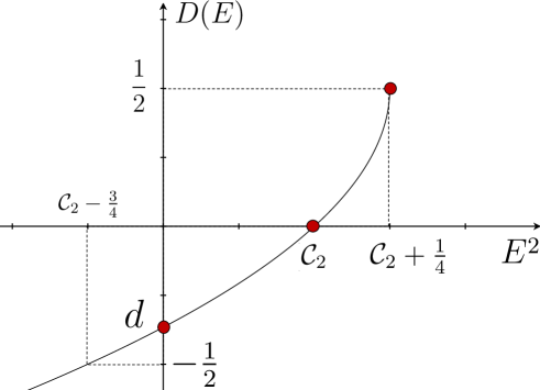
Figure 1: The $D$-function. It is defined in the range $0\leq E^{2}\leq\mathcal{C}_{2}+\frac{1}{4}$ and decreasing monotonically from the UV to the IR.

To summarize, if conformal quantum mechanics dual to the AdS₂ has the vacuum $|\Omega\rangle$ and a complete orthonormal set of energy eigenstates $|E\rangle$ with the averaged scaling dimension (4.17), the energy eigenstate will realize well-behaved unitary evolution at $E^{2}=\mathcal{C}_{2}$ for $-\frac{1}{4}<\mathcal{C}_{2}<\frac{3}{4}$.

Here we would like to argue the physical implications of the $D$-function. It involves two important physical quantities, scaling dimension and energy. In quantum field theory change of scale is described by the RG transformation and the number of degrees of freedom in a physical system decreases along the RG flows from high energy to lower energy. In CFT₂ this can be quantitatively measured by defining a $c$-function [4] which has the following properties:

1. It is a real function of coupling constant $g$ and energy scale $E$ which is defined on the space of theories.

2. It monotonically decreases along the RG flow.

3. It is stationary at the RG fixed point where its value equals the crucial parameter in the CFT.

It is proposed [5] that for even dimensional CFT_d, the Euler characteristic appearing in the trace anomaly provides a $c$-function, which can be evaluated as the expectation value of the trace of the energy-momentum tensor on the sphere $S^{d}$

$$c\sim\int_{S^{d}}\langle T_{\mu}^{\mu}\rangle.$$ (4.23)

We remark that the trace $T^{\mu}_{\mu}$ of the energy momentum tensor is related to the conserved current of the dilatation $D$ as the scale invariance is achieved when the trace of the energy momentum tensor vanishes [24]. This leads us to expect that in conformal quantum mechanics the expectation value $\langle D\rangle$ of the dilatation, which depends on the energy scale $E$, can play a role of a $c$-function. In fact, we see that the $D$-function has the above properties of a $c$-function:

1. The $D$-function is defined on the space of theory as it depends on the Casimir which may involve the coupling constants of the theories considered. For instance, in the DFF-model (3.15) the Casimir invariant is given by the coupling constant $g$ as in (3.18) and the $D$-function is represented by

   $$D(E) =\frac{1-\sqrt{g-4E^{2}+\frac{1}{4}}}{2}.$$ (4.24)

   Since the dimensionless coupling constant $g$ parameterizes the theories, the $D$-function is defined on the space of the theories.

2. Along the flow from the UV to the IR, the energy scale decreases and the $D$-function decreases monotonically with the energy scale $E$

   $$\frac{dD(E)}{dE} =\frac{2E}{\sqrt{1+4(\mathcal{C}_{2}-E^{2})}}\geq 0.$$ (4.25)

   This shows the monotonic flow for the $D$-function.

3. At the fixed point $E=0$ of the flow, it is stationary with its value

   $$D(E=0) =d=\frac{1-\sqrt{1+4\mathcal{C}_{2}}}{2}.$$ (4.26)

   This is the crucial parameter in conformal quantum mechanics, that is the scaling dimension (3.15) of the vacuum state.

Therefore the $D$-function exhibits analogous properties as a $c$-function. It supports the irreversibility of the flow from the UV to the IR in conformal quantum mechanics. At the fixed point it becomes the scaling dimension $d$ of the vacuum that encodes the theory considered. As dimension conceptually measures certain properties of an object that is independent from other objects, the $D$-function as an averaged scaling dimension of energy eigenstates, including the scaling dimension $d$ of the vacuum counts the number of degrees of freedom in a similar way as a $c$-function.

5 Bounds on Scaling Dimensions

Now we want to consider a dynamical realization of conformal group in quantum mechanics. We shall postulate the existence of primary operators transforming as representations of the conformal algebra

$$\left(T(g)\mathcal{O}\right)_{\alpha}(t) =S_{\alpha\beta}(g,t)\mathcal{O}_{\beta}(g^{-1}t)$$ (5.1)

where $g$ acts on time coordinate $t$ as (2.16) and $T(g)$ is the representation matrix. It follows from (5.1) that $S_{\alpha\beta}(g,0)$ should be a representation of the stability subgroup at time $t=0$. According to the infinitesimal transformation (2.17) this subgroup is given by the dilatation and special conformal transformation. The commutation relation (2.18) reduces to

$$[K,D] =-iK.$$ (5.2)

Every element of the $\mathfrak{sl}(2,\mathbb{R})$ conformal algebra can be constructed by ascribing the time dependence to the generators. From (4.9) we have

$$D(t) =e^{iHt}De^{-iHt}=D-tH,$$ (5.3)

$$K(t) =e^{iHt}Ke^{-iHt}=K-2tD+t^{2}H$$ (5.4)

Assume that

$$H\mathcal{O}(0) =i\dot{\mathcal{O}}(0),$$ (5.5)

$$D\mathcal{O}(0) =i\Delta\mathcal{O}(0),$$ (5.6)

$$K\mathcal{O}(0) =0$$ (5.7)

with $\Delta\in\mathbb{R}$. (5.6) says that the operator $\mathcal{O}(0)$ enjoys a real scaling dimension $\Delta$. According to (5.3) and (5.4) we find that

$$H\mathcal{O}_{\Delta}(t) =i\dot{\mathcal{O}}_{\Delta}(t),$$ (5.8)

$$D\mathcal{O}_{\Delta}(t) =i\left(-t\frac{\partial}{\partial t}+\Delta\right)\mathcal{O}_{\Delta}(t),$$ (5.9)

$$K\mathcal{O}_{\Delta}(t) =i\left(t^{2}\frac{\partial}{\partial t}-2t\Delta\right)\mathcal{O}_{\Delta}(t).$$ (5.10)

Equivalently one can define the primary operators $\mathcal{O}_{\Delta}(t)$ which obey (5.8)-(5.10) by the transformation law

$$\mathcal{O}_{\Delta}(t) \rightarrow\left(\frac{\partial t^{\prime}}{\partial t}\right)^{\Delta}\mathcal{O}_{\Delta}(t^{\prime})=\frac{1}{(ct+d)^{2\Delta}}\mathcal{O}_{\Delta}(t^{\prime})$$ (5.11)

under the finite transformation (2.16).

We will formulate conformal quantum mechanics in terms of the primary operators $\mathcal{O}_{\Delta}(t)$ acting on the vacuum state $|\Omega\rangle$. We assume that each state in the Hilbert space is represented by

$$|\mathrm{state}\rangle =F(G)|\mathcal{O}_{\Delta_{1}}(t_{1})\cdots\mathcal{O}_{\Delta_{n}}(t_{n})\rangle$$ (5.12)

where

$$|\mathcal{O}_{\Delta_{1}}(t_{1})\cdots\mathcal{O}_{\Delta_{n}}(t_{n})\rangle =\mathcal{O}_{\Delta_{1}}(t_{1})\cdots\mathcal{O}_{\Delta_{n}}(t_{n})|\Omega\rangle$$ (5.13)

with $F(G)$ being some function of $G=uH+vD+wK$. Let us examine the expectation values $\langle\mathrm{state}A|\mathrm{state}B\rangle$ constructed as overlaps of the two states $|\mathrm{state}A\rangle$ and $|\mathrm{state}B\rangle$ with the form of (5.12) in the Hilbert space. In this work we will explore the expectation value involving the time-independent primary operators $\mathcal{O}_{\Delta}:=\mathcal{O}_{\Delta}(0)$ and take the conventional choice of the overall constant one which fixes the normalization of $\mathcal{O}_{\Delta}$ as

$$\langle\mathcal{O}_{\Delta}|\mathcal{O}_{\Delta}\rangle =1.$$ (5.14)

Now we would like to extract constraints on the description of the unitary evolution for a certain physical system. To achieve this, one needs to fix its time coordinate $t$ and construct all the physical states in such a way that they fall into the representations of the $\mathfrak{sl}(2,\mathbb{R})$ conformal algebra specified by the vacuum with the eigenvalue of the Casimir invariant $\mathcal{C}_{2}$, i.e. the scaling dimension $d$. Given the normalized primary operators (5.14), this corresponds to the condition

$$\langle\mathcal{O}_{\Delta}|\mathcal{C}_{2}|\mathcal{O}_{\Delta}\rangle =\mathcal{C}_{2}=d(d-1),$$ (5.15)

which ensures the unitary evolution of the states by fixing the eigenvalue of the Casimir invariant. Alternatively, we can write the expectation value (5.15) as

$$\langle\mathcal{O}_{\Delta}|HK-iD-D^{2}|\mathcal{O}_{\Delta}\rangle =\langle\mathcal{O}_{\Delta}|HK|\mathcal{O}_{\Delta}\rangle+(d+\Delta)(d+\Delta+1).$$ (5.16)

Unitarity implies the positivity of the inner product in the Hilbert space. Demanding that $\langle\mathcal{O}_{\Delta}|HK|\mathcal{O}_{\Delta}\rangle=|K|\mathcal{O}_{\Delta}\rangle|^{2}$ is positive definite and combining (5.15) with (5.16), we find a condition

$$(\Delta+2d)(\Delta+1)\leq 0.$$ (5.17)

Together with the preferred range (4.22) under the unitary evolution probed by the $D$-function, we obtain the bounds on scaling dimension of the primary operator and of the vacuum

$$-1 \leq\Delta\leq-2d,$$ (5.18)

$$-\frac{1}{2} \leq d\leq\frac{1}{2}.$$ (5.19)

Similarly we can extract further constraints by rewriting (5.15) as

$$\langle\mathcal{O}_{\Delta}|KH+iD-D^{2}|\mathcal{O}_{\Delta}\rangle =\langle\mathcal{O}_{\Delta}|KH|\mathcal{O}_{\Delta}\rangle+(d+\Delta)(d+\Delta-1).$$ (5.20)

Since $\langle\mathcal{O}_{\Delta}|KH|\mathcal{O}_{\Delta}\rangle=|H|\mathcal{O}_{\Delta}\rangle|^{2}$ is positive definite, we get a condition

$$\Delta(\Delta+2d-1) \leq 0,$$ (5.21)

which gives the additional constraint

$$0\leq\Delta\leq-2d+1.$$ (5.22)

The result is depicted in Figure 2.

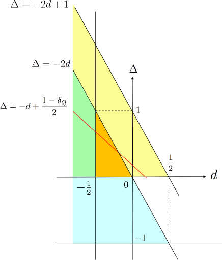
Figure 2: The bound on $(d,\Delta)$ in conformal quantum mechanics. In the orange region the primary operators with the dimension $\Delta$ and the vacuum states with the dimension $d$ are allowed and the red line characterizes the charged physical states coupled to the gauge operators of $\delta_{Q}$. Without the favored condition (5.19) for the unitary evolution of the states, the green region is also allowed.

The primary operators and the vacuum states can exist in the orange region. As a consequence, the allowed range of the scaling dimensions of the physical states $|\mathcal{O}_{\Delta}\rangle$ which are constructed in terms of the vacua and the primary operators is

$$-\frac{1}{2}\leq d+\Delta\leq\frac{1}{2}.$$ (5.23)

It supports the existence of the bosonic scalar with scaling dimension $-\frac{1}{2}$, the fermion with the scaling dimension $0$ and the bosonic auxiliary field with scaling dimension $\frac{1}{2}$ in conformal quantum mechanics, as argued and constructed in the Lagrangian theory. If we relax the condition (5.19) for the favored energy eigenstates $|E\rangle$ under the unitary evolution, which is examined by the $D$-function, the states are allowed in the green region.

Suppose that a theory allows the construction of a conserved charge. In what follows, we will not rely on the Lagrangian, but rather describe a charge as the operator that acts on the state (5.12) and the primary operator (5.11). Let $Q$ be the corresponding charge operator that obeys

$$Q\mathcal{O}_{\Delta} =q\mathcal{O}_{\Delta},$$ (5.24)

$$Q|\Omega\rangle =0,$$ (5.25)

$$[H,Q] =0,$$ (5.26)

$$[D,Q] =i\delta_{Q}Q$$ (5.27)

with $q\in\mathbb{R}$. (5.24) and (5.25) assign the charges such that the primary operator $\mathcal{O}_{\Delta}$ has charge $q$ whereas the vacuum state has no charge. (5.26) implies that the charge operator $Q$ is not dynamical. In the Lagrangian description it would have no kinetic term, so it can be eliminated by its algebraic equation of motion as an auxiliary field. (5.27) gives the scaling dimension $\delta_{Q}$ of the charge operator $Q$. In the following we will focus on the case $\delta_{Q}\geq 0$.

The corresponding symmetry transformation is a global transformation if $\delta_{Q}=0$ because every charge at $t$ is transformed in the same way so that $q$ is a constant charge, which we will call a global charge. For the continuous symmetry an operator can be realized by exponentiating the corresponding global charge. When the theory is generalized by including a $d-1$-dimensional space $M_{d-1}$ separated from time, one may further define higher-form global symmetries and higher-form global charges $Q(M_{d-1})$ [25] by furnishing the scaling dimensions stemming from $M_{d-1}$.

On the other hand, for $\delta_{Q}>0$ we view the symmetry transformation as a local transformation because the charge is a function of time; $q(t)$. In this case $Q$ can enter the Lagrangian and its elimination by the equation of motion and the gauge fixing would gives the Gauss constraint. In the Lagrangian description of quantum mechanics, it is nothing but an auxiliary gauge field. In quantum mechanics, it is the Gauss law operator. Note that the Gauss law constraint is not the identity between operators obeying the canonical commutation relation $[\cdot,\cdot]$ but rather it holds only when acting on the physical states. In fact, it is well known that the Gauss law constraint is incompatible with the canonical commutation relation . Therefore we should not require the Jacobi identity for a canonical commutation relation operation by including the Gauss law operator $Q$. When the theory is generalized by adding a $d-1$-dimensional space $M_{d-1}$, this operator behaves as a vector- or tensor-like operator since it has the non-vanishing scaling dimension. If a theory follows the action principle, it naturally appears in the covariant derivative as a gauge field to make the symmetry manifest. We will refer to the charge operator with $\delta_{Q}>0$ as a gauge operator.

Consider a matrix element

$$\langle\mathcal{O}_{\Delta}|[K,Q]H|\mathcal{O}_{\Delta}\rangle.$$ (5.30)

Since $[K,Q]H=(KH)Q-Q(KH)$ and the both actions of $Q$ on the ket $|\mathcal{O}_{\Delta}\rangle$ and on the bra $\langle\mathcal{O}_{\Delta}|$ produce the same charge $q\in\mathbb{R}$, this should vanish. On the other hand, using the commutation relations (2.18) and (5.24)-(5.27), we find

$$[K,Q]H =2i\delta_{Q}QD-\delta_{Q}^{2}Q+\delta_{Q}Q.$$ (5.31)

Plugging this into (5.30) we get

$$q\delta_{Q}\left(\delta_{Q}-1+2(d+\Delta)\right) =0.$$ (5.32)

For the global charge operator with $\delta_{Q}=0$ the above condition holds and there is no constraint on the primary operator. However, for the gauge operator with $\delta_{Q}>0$ the scaling dimension of the charged primary operator is determined by

$$d+\Delta =\frac{1-\delta_{Q}}{2}.$$ (5.33)

The resulting constrained scaling dimension is illustrated in Figure 2. The red line characterizes the gauge operator. Within the regions (5.23) and (5.19), there exists a bound on the scaling dimension of the gauge operator

$$0<\delta_{Q}\leq 2.$$ (5.34)

This admits the presence of the gauge operators with $\delta_{Q}=1$, which would realize massless spin $s=1$ gauge fields involving photon and gluon, coupled to the physical states with $d+\Delta=0$, i.e. free fermions. Also it is compatible with the gauge operators with $\delta_{Q}=2$, which would show up as massless spin $s=2$ fields involving graviton, coupled to the physical states with $d+\Delta=-\frac{1}{2}$, i.e. free bosonic scalars. On the other hand, the bosonic auxiliary field with $d+\Delta=\frac{1}{2}$ may not couple to the gauge operators.

6 Discussion

In this work we have studied conformal quantum mechanics with the vacuum state and the primary operators. We have shown that a matrix element of the dilatation operator between two energy eigenstates may define a conformal quantum mechanical counterpart of a $c$-function, which we call a $D$-function. Its monotonic decrease from the UV to the IR along the flow supports the universal irreversibility of the RG flow in higher dimensional field theories. At the fixed point of the flow it becomes a crucial parameter $d$, that is the scaling dimension of the vacuum, which specifies the theory, analogous to the central charge in two-dimensional conformal field theories. In addition, we have found new no-go theorems which impose constraints and bounds on scaling dimensions of the primary operator, the vacuum and the gauge operators.

Our results in conformal quantum mechanics should have implications for two-dimensional gravity and black holes via holography. It would be nice to find further applications of our proposed $D$-function in a holographic framework of the RG flow as in higher dimensional conformal field theories in the context of the AdS/CFT correspondence [26, 27]. Also our result may be substantiated by the dS/CFT correspondence [28]. As the radial direction corresponds to time evolution in an asymptotically de Sitter space-time [28, 29], time evolution would be dual to the RG flow. It is discussed [30] that the RG flow may correspond to the instability of the space due to the Hawking emission [31]. When time goes on, the black hole mass would decrease due to the Hawking radiation. Nevertheless, Bianchi and Serlak [32, 33] have recently derived a formula that relates the energy flux and the von Neumann entropy of the Hawking radiation for a two-dimensional black hole, which predicts the possibility of the increase of black hole mass due to the negative energy flux, whereas Abdolrahimi and Page [34] have pointed out some inadequacies in the Bianchi-Smerlak formula. We would like to address these issues via the holographic method in the future work.

Although we have investigated several properties of conformal quantum mechanics, there would be other conformal quantum mechanical models which are beyond the scope of this work. Firstly one can construct other conformal quantum mechanics by considering topological quantum mechanics, which may not obey the unitary evolution for energy eigenstates in our argument. Such theories may have zero Hamiltonian, however, they can appears in the study of topological or BPS protected sector for physical system. For example superconductor and fractional Quantum Hall systems are studied by topological Chern-Simons quantum mechanics [35, 36, 37] and a certain BPS protected sectors are examined by superconformal quantum mechanics [38] (see also [39, 40, 41] and references therein). By relaxing the unitary evolution of physical energy eigenstates, which is taken as the physically preferable conditions in this work, one may find other conformal quantum mechanics which can be used as a physical description.

Meanwhile, even if we focus on the $SL(2,\mathbb{R})$ conformal quantum mechanics, there may exist some quantum mechanical models which are not studied in this work. One possibility is to construct conformal quantum mechanics which does not rely on the existence of vacuum state and of the primary operators. In fact, Chamon, Jackiw, Pi and Santos [42, 17] argue that in the DFF model the unexpected non-primary operator and the non-conformally invariant state conspire with each other to construct the consistent correlation functions.

For many applications of the conformal quantum mechanics, it would be important to proceed with the analysis of correlation functions and to explore stronger constraints by considering additional physical requirement or the presence of additional operators characterizing symmetries in the theory.

Acknowledgements

The author would like to thank C. Cardona, R. Jackiw, G. Dimitrios, D. S. Gupta, K. Hosomichi, S. Kawamoto, Y. Matsuo, S. Pal, D. J. Smith and S. Yamaguchi for useful discussions and comments. The author also thanks the organizers of the Workshop on String and M-theory in Okinawa in Okinawa for providing a stimulating environment during the completion of the work. The author is supported by MOST under the Grant No.105-2811-066.

References

- [1] S. Ferrara, A. F. Grillo, and R. Gatto, “Tensor representations of conformal algebra and conformally covariant operator product expansion,” Annals Phys. 76 (1973) 161–188.
- [2] A. M. Polyakov, “Nonhamiltonian approach to conformal quantum field theory,” Zh. Eksp. Teor. Fiz. 66 (1974) 23–42.
- [3] G. Mack, “Duality in quantum field theory,” Nucl. Phys. B118 (1977) 445–457.
- [4] A. B. Zamolodchikov, “Irreversibility of the Flux of the Renormalization Group in a 2D Field Theory,” JETP Lett. 43 (1986) 730–732. [Pisma Zh. Eksp. Teor. Fiz.43,565(1986)].
- [5] J. L. Cardy, “Is There a c Theorem in Four-Dimensions?,” Phys. Lett. B215 (1988) 749–752.
- [6] R. C. Myers and A. Sinha, “Holographic c-theorems in arbitrary dimensions,” JHEP 01 (2011) 125, 1011.5819.
- [7] D. L. Jafferis, “The Exact Superconformal R-Symmetry Extremizes Z,” JHEP 05 (2012) 159, 1012.3210.
- [8] H. Casini, M. Huerta, and R. C. Myers, “Towards a derivation of holographic entanglement entropy,” JHEP 05 (2011) 036, 1102.0440.
- [9] Z. Komargodski and A. Schwimmer, “On Renormalization Group Flows in Four Dimensions,” JHEP 12 (2011) 099, 1107.3987.
- [10] H. Elvang, D. Z. Freedman, L.-Y. Hung, M. Kiermaier, R. C. Myers, and S. Theisen, “On renormalization group flows and the a-theorem in 6d,” JHEP 10 (2012) 011, 1205.3994.
- [11] B. Grinstein, D. Stone, A. Stergiou, and M. Zhong, “Challenge to the Theorem in Six Dimensions,” Phys. Rev. Lett. 113 (2014), no. 23 231602, 1406.3626.
- [12] S. Weinberg and E. Witten, “Limits on Massless Particles,” Phys. Lett. B96 (1980) 59–62.
- [13] V. de Alfaro, S. Fubini, and G. Furlan, “Conformal Invariance in Quantum Mechanics,” Nuovo Cim. A34 (1976) 569.
- [14] F. Strocchi, “Gauge Invariance and Weyl-polymer Quantization,” Lect. Notes Phys. 904 (2016) 1–97.
- [15] T. Okazaki, “Whittaker vector, Wheeler-DeWitt equation, and the gravity dual of conformal quantum mechanics,” Phys. Rev. D92 (2015), no. 12 126010, 1510.04759.
- [16] S. Pal and B. Grinstein, “Weyl Consistency Conditions in Non-Relativistic Quantum Field Theory,” JHEP 12 (2016) 012, 1605.02748.
- [17] R. Jackiw and S. Y. Pi, “Conformal Blocks for the 4-Point Function in Conformal Quantum Mechanics,” Phys. Rev. D86 (2012) 045017, 1205.0443. [Erratum: Phys. Rev.D86,089905(2012)].
- [18] S. Gubser, I. R. Klebanov, and A. M. Polyakov, “Gauge theory correlators from noncritical string theory,” Phys.Lett. B428 (1998) 105–114, hep-th/9802109.
- [19] E. Witten, “Anti-de Sitter space and holography,” Adv.Theor.Math.Phys. 2 (1998) 253–291, hep-th/9802150.
- [20] P. Breitenlohner and D. Z. Freedman, “Positive Energy in anti-De Sitter Backgrounds and Gauged Extended Supergravity,” Phys. Lett. B115 (1982) 197–201.
- [21] P. Breitenlohner and D. Z. Freedman, “Stability in Gauged Extended Supergravity,” Annals Phys. 144 (1982) 249.
- [22] L. Mezincescu and P. K. Townsend, “Stability at a Local Maximum in Higher Dimensional Anti-de Sitter Space and Applications to Supergravity,” Annals Phys. 160 (1985) 406.
- [23] B. Pioline and J. Troost, “Schwinger pair production in AdS2,” JHEP 03 (2005) 043, hep-th/0501169.
- [24] S. R. Coleman and R. Jackiw, “Why dilatation generators do not generate dilatations?,” Annals Phys. 67 (1971) 552–598.
- [25] D. Gaiotto, A. Kapustin, N. Seiberg, and B. Willett, “Generalized Global Symmetries,” JHEP 02 (2015) 172, 1412.5148.
- [26] D. Z. Freedman, S. S. Gubser, K. Pilch, and N. P. Warner, “Renormalization group flows from holography supersymmetry and a c theorem,” Adv. Theor. Math. Phys. 3 (1999) 363–417, hep-th/9904017.
- [27] R. C. Myers and A. Sinha, “Seeing a c-theorem with holography,” Phys. Rev. D82 (2010) 046006, 1006.1263.
- [28] A. Strominger, “The dS/CFT correspondence,” JHEP 10 (2001) 034, hep-th/0106113.
- [29] V. Balasubramanian, J. de Boer, and D. Minic, “Notes on de Sitter space and holography,” Class. Quant. Grav. 19 (2002) 5655–5700, hep-th/0207245. [Annals Phys.303,59(2003)].
- [30] E. Halyo, “On the Cardy-Verlinde formula and the de Sitter/CFT correspondence,” JHEP 03 (2002) 009, hep-th/0112093.
- [31] S. W. Hawking, “Particle Creation by Black Holes,” Commun. Math. Phys. 43 (1975) 199–220. [,167(1975)].
- [32] E. Bianchi and M. Smerlak, “Entanglement entropy and negative energy in two dimensions,” Phys. Rev. D90 (2014), no. 4 041904, 1404.0602.
- [33] E. Bianchi and M. Smerlak, “Last gasp of a black hole: unitary evaporation implies non-monotonic mass loss,” Gen. Rel. Grav. 46 (2014), no. 10 1809, 1405.5235.
- [34] S. Abdolrahimi and D. N. Page, “Hawking Radiation Energy and Entropy from a Bianchi-Smerlak Semiclassical Black Hole,” Phys. Rev. D92 (2015), no. 8 083005, 1506.01018.
- [35] N. S. Manton, “First order vortex dynamics,” Annals Phys. 256 (1997) 114–131, hep-th/9701027.
- [36] A. P. Polychronakos, “Quantum Hall states as matrix Chern-Simons theory,” JHEP 04 (2001) 011, hep-th/0103013.
- [37] N. Dorey, D. Tong, and C. Turner, “Matrix model for non-Abelian quantum Hall states,” Phys. Rev. B94 (2016), no. 8 085114, 1603.09688.
- [38] S. Fubini and E. Rabinovici, “SUPERCONFORMAL QUANTUM MECHANICS,” Nucl.Phys. B245 (1984) 17.
- [39] R. Britto-Pacumio, J. Michelson, A. Strominger, and A. Volovich, “Lectures on superconformal quantum mechanics and multiblack hole moduli spaces,” hep-th/9911066.
- [40] S. Fedoruk, E. Ivanov, and O. Lechtenfeld, “Superconformal Mechanics,” J. Phys. A45 (2012) 173001, 1112.1947.
- [41] T. Okazaki, Superconformal Quantum Mechanics from M2-branes. PhD thesis, Caltech, 2015. 1503.03906.
- [42] C. Chamon, R. Jackiw, S.-Y. Pi, and L. Santos, “Conformal quantum mechanics as the CFT1 dual to AdS2,” Phys. Lett. B701 (2011) 503–507, 1106.0726.