Discontinuous motions of limit sets

Abstract.

We characterise completely when limit sets, as parametrised by Cannon-Thurston maps, move discontinuously for a sequence of algebraically convergent quasi-Fuchsian groups.

1. Introduction

In [Question 14] of [Thu82], Thurston raised a question about continuous motions of limit sets under algebraic deformations of Kleinian groups. This problem was formulated more precisely in [MS13, MS17] taking into account topologies of convergence of Kleinian groups and a parametrisation of limit sets using Cannon-Thurston maps [CT07, Mj14a]. The questions can be stated as follows.

Question 1.1.

[Thu82, MS13, MS17]

1. If a sequence of isomorphic Kleinian groups $(G_{n})$ converges to $G_{\infty}$ algebraically then do the corresponding Cannon-Thurston maps converge pointwise?

2. If $(G_{n})$ converges to $G_{\infty}$ strongly then do the corresponding Cannon-Thurston maps converge uniformly?

It was established, in [MS17] and [Mj17a] (crucially using technology developed in [Mj14a], [Mj17b]) that the second question has an affirmative answer. The answer to the first question has turned out to be considerably subtler. Indeed, interesting examples of both continuity and discontinuity occur naturally:

1. In [MS13], it was shown that if the geometric limit $\Gamma$ of $(G_{n})$ is geometrically finite, then the answer to Question 1.1 (1) is affirmative. In particular, this is true for the examples given by Kerckhoff-Thurston in [KT90].

2. On the other hand, it was shown in [MS17], that for certain examples of quasi-Fuchsian groups converging to geometrically infinite groups constructed by Brock [Bro01], the answer to Question 1.1 (1) is negative.

In this paper, we shall complete the answer to Question 1.1 (1) for sequences of quasi-Fuchsian groups by characterising precisely when limit sets move discontinuously, i.e. we isolate the fairly delicate conditions that ensure the discontinuity phenomena illustrated in [MS17] for Brock’s examples. In order to do this, we need to understand possible geometric limits of sequences of Kleinian surface groups. The necessary technology was developed in [OS] and [Ohs]. In particular, it was shown there that there exists an embedding of any such geometric limit into $S\times(-1,1)$. In the following, we shall mainly refer to [Ohs], where a simplified proof for convergent sequences is given, rather than to [OS].

Let $(\rho_{n}:\pi_{1}(S)\rightarrow\operatorname{PSL}_{2}\mathbb{C})$ be a sequence of quasi-Fuchsian groups converging algebraically to $\rho_{\infty}:\pi_{1}(S)\rightarrow\operatorname{PSL}_{2}\mathbb{C}$, where $S$ is a hyperbolic surface of finite area. We set $G_{n}=\rho_{n}(\pi_{1}(S))$ and $G_{\infty}=\rho_{\infty}(\pi_{1}(S))$. Suppose that $(G_{n})$ converges geometrically to a Kleinian group $\Gamma$. In what follows, we need to consider ends of the non-cuspidal part $({\mathbb{H}}^{3}/G_{\infty})_{0}$ (resp. $({\mathbb{H}}^{3}/\Gamma)_{0}$) of the algebraic (resp. geometric) limit. For an end $e$ of either $({\mathbb{H}}^{3}/G_{\infty})_{0}$ or $({\mathbb{H}}^{3}/\Gamma)_{0}$, if there is a $\mathbb{Z}$-cusp neighbourhood whose boundary $A$ has an end tending to $e$, we say that $A$ (or the corresponding $\mathbb{Z}$-cusp neighbourhood) abuts on $e$. Abusing terminology, we also say that for a neighbourhood $E$ of $e$ the annulus $A$ or the corresponding cusp neighbourhood abuts on $E$ in this situation. Before stating the main theorem of this paper, we shall introduce some terminology.

We first explain what it means for a simply degenerate end $e$ of $({\mathbb{H}}^{3}/G_{\infty})_{0}$ to be coupled. See figure below. We shall describe this condition more precisely in §2.7, and we just give a sketch here. Let $E$ be a neighbourhood of $e$ homeomorphic to $\Sigma\times\mathbb{R}$ for an essential subsurface $\Sigma$ of $S$. The neighbourhood $E$ can be taken to project homeomorphically to a neighbourhood $\bar{E}$ of an end $\bar{e}$ of $({\mathbb{H}}^{3}/\Gamma)_{0}$, the non-cuspidal part of the geometric limit. The end $\bar{e}$ is required to satisfy the following. There is another end $\bar{e}^{\prime}$ of $({\mathbb{H}}^{3}/\Gamma)_{0}$, simply degenerate or wild, called a partner of $\bar{e}$. The ends $\bar{e}^{\prime}$ and $\bar{e}$ are related as follows. The end $\bar{e}^{\prime}$ has a neighbourhood $\bar{E}^{\prime}$ such that if we pull back $\bar{E}$ and $\bar{E}^{\prime}$ by approximate isometries to ${\mathbb{H}}^{3}/G_{n}$ for large $n$, then their images are both contained in a submanifold of the form $\Sigma\times(0,1)$, where $\operatorname{Fr}\Sigma\times(0,1)$ lies on the boundaries of Margulis tubes, and $\Sigma\times\{t\}$ is incompressible. Fig. 1 is a schematic representation of ${\mathbb{H}}^{3}/G_{n}$ and the second is a schematic representation of the limit $({\mathbb{H}}^{3}/\Gamma)_{0}$. Note that $\bar{E}^{\prime}$ is not required to be homeomorphic to $\Sigma\times\mathbb{R}$, as indicated by the semicircular bump in the middle of $\bar{E}^{\prime}$ in Fig. 2. In fact $\bar{E}^{\prime}$ may only be homeomorphic to $\Sigma^{\prime}\times\mathbb{R}$ for some essential subsurface $\Sigma^{\prime}$ of $S$, which shares a boundary component with $\Sigma$.

Figure 1. Schematic representation of ${\mathbb{H}}^{3}/G_{n}$

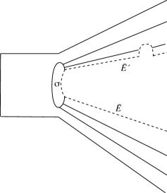
Figure 2. Schematic representation of coupled ends $\bar{E},\bar{E}^{\prime}$ in $({\mathbb{H}}^{3}/\Gamma)_{0}$ with conjoining cusp corresponding to $\sigma$

A $\mathbb{Z}$-cusp corresponding to a parabolic curve $\sigma$, abutting on both an end $\bar{E}$ and its partner $\bar{E}^{\prime}$ is said to conjoin $\bar{E}$ and $\bar{E}^{\prime}$ or $e,e^{\prime}$. Such a cusp will sometimes be referred to simply as a conjoining cusp (see Fig. 2). Such a conjoining cusp is called untwisted if the Dehn twist parameters of the Margulis tubes corresponding to the $\mathbb{Z}$-cusp are bounded uniformly all along the sequence $(\rho_{n})$.

Let $\mu$ be the ending lamination of the end $\bar{e}$. A crown domain for $(\mu,\sigma)$ is said to be well-approximated if it is realised in $\bar{E}^{\prime}$ (with respect to the marking determined by approximate isometries). See §2.7 for a more precise definition. We now state the main theorem of this paper.

Theorem 1.2.

Let $c_{n}:S^{1}(=\Lambda_{\pi_{1}(S)})\rightarrow\Lambda_{\rho_{n}(\pi_{1}(S))}$ denote the Cannon-Thurston maps for the quasi-Fuchsian representations $\rho_{n}\ (n=1,\cdots,\infty)$. Then $(c_{n})$ does not converge pointwise to $c_{\infty}$ if and only if all of Conditions (1)-(3) below are satisfied.

1. The algebraic limit has a coupled end $e$ with a partner $e^{\prime}$.

2. There is an untwisted cusp $\mathbb{Z}$-cusp corresponding to a parabolic curve $\sigma$, conjoining $e,e^{\prime}$.

3. Let $\mu$ be the ending lamination of the end $\bar{e}$. There exists a well-approximated crown domain for $(\mu,\sigma)$.

Remark 1.3.

Condition 1 is concerned with the type of geometric limit. However, Conditions 2 and 3 deal with the manner in which the sequence converges geometrically.

In fact Theorem 1.2 shows that we can construct examples of two sequences of quasi-Fuchsian groups having the same geometric limit and also the same algebraic limit; however, the sequence of Cannon-Thurston maps have radically different behaviour. For one sequence, the Cannon-Thurston maps converge pointwise, for the other they fail to do so.

It is this subtlety that is captured by the somewhat technical nature of the statement of Theorem 1.2 above.

We shall also characterise the points where this discontinuity occurs (see Theorem 2.17). These turn out to be exactly the tips of crown domains as in [MS17].

Theorem 1.4.

In the setting of Theorem 1.2, suppose that

1. $({\mathbb{H}}^{3}/G_{\infty})_{0}$ has a coupled simply degenerate end $e$ with ending lamination $\lambda$,

2. an untwisted $\mathbb{Z}$-cusp corresponding to a parabolic curve $s$ abutting on the image of $e$ in $({\mathbb{H}}^{3}/\Gamma)_{0}$,

3. there exists a well approximated crown domain for $(\lambda,s)$.

Then for $\zeta\in S^{1}$, the images $c_{n}(\zeta)$ do not converge to $c_{\infty}(\zeta)$ if and only if $\zeta$ is a tip of a crown domain $C$ for $(\mu,\sigma)$, where

1. $\mu\cup\sigma$ is contained in either the union of the lower parabolic curves and the lower ending laminations (denoted by $\lambda_{-}$), or the union of the upper parabolic curves and the upper ending laminations, (denoted by $\lambda_{+}$);

2. the crown domain $C$ is well approximated;

3. the simple closed curve $\sigma$ corresponds to an untwisted conjoining cusp abutting on the projection of the end in $({\mathbb{H}}^{3}/\Gamma)_{0}$ for which $\mu$ is the ending lamination.

2. Preliminaries

2.1. Some basic material for hyperbolic 3-manifolds

Let $(S,m)$ be a complete hyperbolic surface of finite area, possibly with cusps. A geodesic lamination on $(S,m)$ is a closed subset of $S$ which is a disjoint union of simple geodesics. The notion of geodesic lamination depends on the hyperbolic metric $m$. However, given any geodesic lamination $\lambda$ on $(S,m)$ and any complete hyperbolic metric $m^{\prime}$ on $S$, there is a unique geodesic lamination $\lambda^{\prime}$ on $(S,m^{\prime})$ which is ambient isotopic to $\lambda$.

For a surface $S$ as above and a hyperbolic 3-manifold $M$, a continuous $f\colon S\to M$ is said to be a pleated surface if there is a complete hyperbolic metric $m$ on $S$ and a geodesic lamination $\lambda$ on $(S,m)$ such that $f$ maps each leaf of $\lambda$ to a geodesic, and each component of $S\setminus\lambda$ totally geodesically. The geodesic lamination $\lambda$ is called the pleating locus of the pleated surface $f\colon S\to M$. A geodesic lamination $\lambda$ on $S$ (with some fixed complete hyperbolic metric) is said to be realised by a pleated surface $f\colon S\to M$ if $\lambda$ is ambient isotopic to the pleating locus of the pleated surface $f\colon S\to M$.

2.2. Relative hyperbolicity and electrocution

We refer the reader to [Far98] and [Bow12] for generalities on relative hyperbolicity and to [Mj11] and [Mj14a] for the notions of electrocution and electro-ambient paths. We shall briefly recall the notion of electro-ambient quasi-geodesics, c.f. [Mj14a]. Let $(X,d_{X})$ be a $\delta$-hyperbolic metric space. Bowditch showed in [Bow12] that if there are constants $C,D$ and a family $\mathcal{K}$ of $D$-separated, $C$-quasi-convex sets in $X$, then $X$ is (weakly) hyperbolic relative to $\mathcal{K}$. Now let $\mathcal{H}$ be a collection of $C$-quasi-convex sets in $(X,d_{X})$, without assuming the $D$-separated condition. Let ${{\mathcal{E}}(X,{\mathcal{H}})}$ denote the space obtained by electrocuting the elements of $\mathcal{H}$ in $X$: this space is a union of $X$ and $\sqcup_{H\in\mathcal{H}}H\times[0,1/2]$, where $H\times\{0\}$ is identified with $H$ in $X$, each $\{h\}\times[0,1/2]$ is isometric to $[0,1/2]$, and $H\times\{1/2\}$ is equipped with the zero metric. Since $\{H\times\{1/2\}\}$ is $1$-separated, we can apply Bowditch’s result, and see that ${{\mathcal{E}}(X,{\mathcal{H}})}$ is Gromov hyperbolic.

Let $\alpha=[a,b]$ be a geodesic in $(X,d_{X})$, and $\beta$ an electric quasi-geodesic without backtracking joining $a,b$ in ${{\mathcal{E}}(X,{\mathcal{H}})}$, i.e. an electric quasi-geodesic which does not return to an element $H\in{\mathcal{H}}$ after leaving it. We further assume that the intersection of $\beta$ and $H\times(0,1/2)$ is either empty or a disjoint union of open arcs of the form $\{h\}\times(0,1/2)$. We parametrise $\beta$, and consider the maximal subsegments of $\beta$ contained entirely in some $H\times\{1/2\}$ (for some $H\in\mathcal{H}$). We extend each such maximal subsegment by adjoining ‘vertical’ subsegments (of the form $h\times[0,1/2])$ in $\beta$ at its endpoints to obtain a path of the form $\{p\}\times[0,1/2]\cup[p,q]\times\{1/2\}\cup\{q\}\times[0,1/2]$. We call these subpaths of $\beta$ extended maximal subsegments. We replace each extended maximal subsegment in $\beta$ by a geodesic path in $(X,d_{X})$ joining the same endpoints.

The resulting path $\beta_{q}$ is called an electro-ambient representative of $\beta$ in $X$. Also, if $\beta$ is an electric $P$-quasi-geodesic without backtracking (in ${\mathcal{E}}(X,{\mathcal{H}})$), then $\beta_{q}$ is called an electro-ambient $P$-quasi-geodesic. If $\beta$ is an electric geodesic without backtracking, then $\beta_{q}$ is simply called an electro-ambient quasi-geodesic. The following lemma says that hyperbolic geodesics do not go far from electro-ambient quasi-geodesic realisations.

Lemma 2.1.

([Kla99, Proposition 4.3], [Mj11, Lemma 3.10] and [Mj14a, Lemma 2.5]) For given non-negative numbers $\delta$, $C$ and $P$, there exists $R$ such that the following holds:
Let $(X,d_{X})$ be a $\delta$-hyperbolic metric space and $\mathcal{H}$ a family of $C$-quasi-convex subsets of $X$. Let $({\mathcal{E}}(X,{\mathcal{H}}),d_{e})$ denote the electric space obtained by electrocuting the elements of $\mathcal{H}$. Then, $({\mathcal{E}}(X,{\mathcal{H}}),d_{e})$ is Gromov hyperbolic, and if $\alpha,\beta_{q}$ denote respectively a geodesic arc with respect to $d_{X}$, and an electro-ambient $P$-quasi-geodesic with the same endpoints in $X$, then $\alpha$ lies in the $R$-neighbourhood of $\beta_{q}$ with respect to $d_{X}$.

2.3. Cannon-Thurston Maps

We shall review known facts about Cannon-Thurston maps focusing on the case of interest in this paper. Let $(Y,{d_{Y}})$ be a Cayley graph of $\pi_{1}(S)$ for $S$ a closed surface of genus at least 2 with respect to some finite generating system, and set $X={\mathbb{H}}^{3}$. By adjoining the Gromov boundaries $\partial{X}(=S^{2})$ and $\partial{Y}(=S^{1})$ to $X$ and $Y$ respectively, we obtain their compactifications $\widehat{X}$ and $\widehat{Y}$ respectively.

Suppose that $\pi_{1}(S)$ acts on ${\mathbb{H}}^{3}$ by isometries as a Kleinian group $G$ via an isomorphism $\rho\colon\pi_{1}(S)\to G$, and let $i:Y\rightarrow X$ be a $\pi_{1}(S)$-equivariant injection.

Definition 2.2.

A Cannon-Thurston map $\hat{i}$ (for $\rho$) from $\widehat{Y}$ to $\widehat{X}$ is a continuous extension of $i$.

The image of $\hat{i}$ restricted to $\partial Y$ coincides with the limit set of $G$. It is easy to see if a Cannon-Thurston map exists, it is unique. The notion of Cannon-Thurston map can be easily extended to the case where $S$ is a hyperbolic surface of finite area. In this situation, it is a $\pi_{1}(S)$-equivariant continuous map from the relative (or Bowditch) boundary relative to the cusp subgroups, $\partial_{\infty}\widetilde{S}=\partial_{\infty}{\mathbb{H}}^{2}=S^{1}$, onto the limit set in $S^{2}$. The first author [Mj14b] showed that for any Kleinian group isomorphic to a surface group (possibly with punctures), a Cannon-Thurston map always exists, and gave the following characterisation of non-injective points. Recall that an isomorphism from a Kleinian group to another Kleinian group is said to be weakly type-preserving when every parabolic element is sent to a parabolic element.

Theorem 2.3.

[Mj14b] Let $S={\mathbb{H}}^{2}/F$ be a (possibly punctured) hyperbolic surface of finite area. Let $\rho:F\rightarrow\operatorname{PSL}_{2}\mathbb{C}$ be a weakly type-preserving discrete faithful representation with image $G$. Let $\lambda_{1}$ be the union of parabolic curves and ending laminations for upper ends and $\lambda_{2}$ that of the lower ends, one (or both) of which might be empty. We regard $\lambda_{1}$ and $\lambda_{2}$ as geodesic laminations on $S$.

For $k=1,2$, let ${\mathcal{R}}_{k}$ denote the relation on $\partial_{\infty}{\mathbb{H}}^{2}$ defined as follows: $\xi{\mathcal{R}}_{k}\eta$ if and only if $\xi$ and $\eta$ are either ideal endpoints of the same leaf of $\tilde{\lambda}_{k}$, or ideal boundary points of a complementary ideal polygon of $\tilde{\lambda}_{k}$, where $\tilde{\lambda}_{k}$ is the preimage of $\lambda_{k}$ in ${\mathbb{H}}^{2}$. Denote the transitive closure of ${\mathcal{R}}_{1}\cup{\mathcal{R}}_{2}$ by ${\mathcal{R}}$. Let $\hat{i}_{\rho}:\partial{F}\to\Lambda_{G}$ be the Cannon-Thurston-map for $\rho$. Then $\hat{i}(\xi)=\hat{i}(\eta)$ for $\xi,\eta\in\partial_{\infty}{\mathbb{H}}^{2}$ if and only if $\xi{\mathcal{R}}\eta$.

Remark 2.4.

When $S$ has punctures, ${\mathcal{R}}$ is strictly larger than ${\mathcal{R}}_{1}\cup{\mathcal{R}}_{2}$. In fact, a vertex of a complementary ideal polygon of $\tilde{\lambda}_{1}$ containing a lift $p$ of a puncture is related by ${\mathcal{R}}$, but not by ${\mathcal{R}}_{1}\cup{\mathcal{R}}_{2}$, to any vertex of a complementary ideal polygon of $\tilde{\lambda}_{2}$ containing $p$.

2.4. Algebraic and Geometric Limits

Let $(\rho_{n}:G\rightarrow\operatorname{PSL}_{2}\mathbb{C})$ be a sequence of weakly type-preserving, discrete, faithful representations of a fixed finitely generated torsion-free group $G$ converging to a discrete, faithful representation $\rho_{\infty}\colon G\rightarrow\operatorname{PSL}_{2}\mathbb{C}$. Also assume that $(\rho_{n}(G))$ converges to a Kleinian group $\Gamma$ as a sequence of closed subsets of $\operatorname{PSL}_{2}\mathbb{C}$ in the Hausdorff topology. Then $\rho_{\infty}(G)$ is called the algebraic limit of the sequence and $\Gamma$ the geometric limit of the sequence $(\rho_{n}(G))$. If $\rho_{\infty}(G)=\Gamma$, we say that the limit is strong. We note that throughout this paper, when we talk about algebraic and geometric limits, we consider a sequence of representation, and not a sequence of conjugacy classes of representations.

There is a more geometric way to think of geometric limits (see [Thu80] and [CEG87]). A sequence of manifolds with basepoints $\{(N_{i},x_{i})\}$ is said to converge geometrically to a manifold with basepoint $(N,x_{\infty})$ if for any $R>0$ and $K>1$, there exist $i_{0}(R,K)>0$ and compact submanifolds $C_{i}\subset N_{i}$ and $C\subset N$ containing $R$-balls around $x_{i}$ and $x_{\infty}$ respectively, such that there exist $K$-bi-Lipschitz maps $h_{i}\colon C_{i}\to C$ for all $i\geq i_{0}(R)$. A sequence of Kleinian groups $(G_{n})$ converges geometrically to $\Gamma$ if and only if for a fixed basepoint $x\in{\mathbb{H}}^{3}$ and its projections $x_{n}$ and $x_{\infty}$ in ${\mathbb{H}}^{3}/G_{n}$ and ${\mathbb{H}}^{3}/\Gamma$, the sequence $\{({\mathbb{H}}^{3}/G_{n},x_{n})\}$ converges geometrically to $({\mathbb{H}}^{3}/\Gamma,x_{\infty})$.

2.5. Criteria for Uniform/Pointwise convergence

We recall some material from [MS13, MS17]. Let $G$ be a fixed finitely generated Kleinian group, and $(\rho_{n}(G)=G_{n})$ a weakly type-preserving sequence of Kleinian groups converging algebraically to $G_{\infty}=\rho_{\infty}(G)$. Also fix a basepoint $o_{{\mathbb{H}}^{3}}\in{\mathbb{H}}^{3}$. Let $d_{G}$ denote the distance in a Cayley graph of $G$ and $d$ the distance in ${\mathbb{H}}^{3}$. Also $[g,h]$ denotes a geodesic in $G$ joining $g$ with $h$, and $[\rho_{n}(g)(o_{{\mathbb{H}}^{3}}),\rho_{n}(h)(o_{{\mathbb{H}}^{3}})]$ denotes a geodesic in ${\mathbb{H}}^{3}$ joining $\rho_{n}(g)(o_{{\mathbb{H}}^{3}})$ with $\rho_{n}(h)(o_{{\mathbb{H}}^{3}})$.

Definition 2.5.

The sequence $(\rho_{n})$ is said to have the Uniform Embedding of Points property (UEP for short) if there exists a non-negative function $f(N)$, with $f(N)\rightarrow\infty$ as $N\rightarrow\infty$, such that for all $g\in\Gamma$, $d_{\Gamma}(1,g)\geq N$ implies $d(\rho_{n}(g)(o_{{\mathbb{H}}^{3}}),o_{{\mathbb{H}}^{3}})\geq f(N)$ for all $n=1,\cdots,\infty$.

The sequence $(\rho_{n})$ is said to have the Uniform Embedding of Pairs of Points property (UEPP for short) if there exists a non-negative function $f(N)$, with $f(N)\rightarrow\infty$ as $N\rightarrow\infty$, such that for all $g,h\in\Gamma$, $d_{\Gamma}(1,[g,h])\geq N$ implies $d([\rho_{n}(g)(o_{{\mathbb{H}}^{3}}),\rho_{n}(h)(o_{{\mathbb{H}}^{3}})],o_{{\mathbb{H}}^{3}})\geq f(N)$ for all $n=1,\ldots,\infty$.

The property UEP is used in [MS13] to give a sufficient criterion to ensure that algebraic convergence is also geometric. The property UEPP is used to give the following criterion for proving uniform convergence of Cannon-Thurston maps.

Proposition 2.6 ([MS13]).

Let $\Gamma$ be a geometrically finite Kleinian group and let $\rho_{n}:\Gamma\to G_{n}$ be weakly type-preserving isomorphisms to Kleinian groups. Suppose that $(\rho_{n})$ converges algebraically to a representation $\rho_{\infty}$. If $(\rho_{n})$ satisfies UEPP, the corresponding Cannon-Thurston maps converge uniformly.

Notation: We shall henceforth fix a complete hyperbolic structure of finite area on $S$ and a Fuchsian group $G$ corresponding to the hyperbolic structure. The limit set $\Lambda_{G}$ is homeomorphic to $S^{1}$. Similarly, $\Lambda_{G_{n}}$ will denote the limit set of $G_{n}$ setting $G_{n}=\rho_{n}(G)$. For each $G_{n}$ $(n\in\mathbb{N}\text{ or }n=\infty)$, we shall denote the corresponding Cannon-Thurston map by $c_{n}:S^{1}=\Lambda_{G}\rightarrow\Lambda_{G_{n}}$.

For pointwise convergence of Kleinian surface groups, a weaker condition called EPP is sufficient. This condition depends on points of $\Lambda_{G}$.

Proposition 2.7 ([MS13]).

Let $G\cong\pi_{1}(S)$ be a Fuchsian group corresponding to a hyperbolic surface $S$ of finite area. Take $\xi\in\Lambda_{G}=S^{1}_{\infty}$ and let $[o_{{\mathbb{H}}^{2}},\xi)$ be a geodesic ray in ${\mathbb{H}}^{2}$ from a fixed basepoint $o_{{\mathbb{H}}^{2}}$ to $\xi$. Let $o_{{\mathbb{H}}^{3}}\in{\mathbb{H}}^{3}$ be a fixed basepoint in ${\mathbb{H}}^{3}$.

1. Suppose that $(\rho_{n}:G\rightarrow\operatorname{PSL}_{2}\mathbb{C})$ is a sequence of weakly type-preserving discrete faithful representations converging algebraically to $\rho_{\infty}:G\rightarrow\operatorname{PSL}_{2}\mathbb{C}$. Set $G_{n}=\rho_{n}(G),n=1,\cdots,\infty$ and $M_{n}={\mathbb{H}}^{3}/G_{n}$.

2. Let $\phi_{n}:S\to M_{n}$ be an incompressible embedding inducing $\rho_{n}$ at the level of fundamental groups. Let $\Phi_{n}:{\mathbb{H}}^{2}\to{\mathbb{H}}^{3}$ be a lift of $\phi_{n}$ (in particular, $\Phi_{n}$ is an embedding).

Then the Cannon-Thurston maps for the $\rho_{n}$ converge to the Cannon-Thurston map for $\rho_{\infty}$ at $\xi$ if
EPP: There exists a proper function $g:{\mathbb{N}}\to{\mathbb{N}}$ such that for any geodesic subsegment $[a,b]$ of the ray $[o_{{\mathbb{H}}^{2}},\xi)\subset{\mathbb{H}}^{2}$ lying outside $B_{N}(o_{{\mathbb{H}}^{2}})$ (the $N$-ball in ${\mathbb{H}}^{2}$ about $o_{{\mathbb{H}}^{2}}$), the geodesic in ${\mathbb{H}}^{3}$ joining $\Phi_{n}(a)$ with $\Phi_{n}(b)$ lies outside $B_{g(N)}(o_{{\mathbb{H}}^{3}})$, (the $g(N)$-ball about $o_{{\mathbb{H}}^{3}}\in{\mathbb{H}}^{3}$).

2.6. Models of Ends of Geometric Limits of Surface Groups

We recall some material from [Ohs], where a simplified analysis of geometric limits of algebraically convergent quasi-Fuchsian groups is given. This is a special case of a more general result in [OS], but will suffice for our purposes.

Let $(\rho_{n})$ be a sequence of quasi-Fuchsian representations of $\pi_{1}(S)$ converging to $\rho_{\infty}$ algebraically. Set $G_{n}=\rho_{n}(\pi_{1}(S))$ and $G_{\infty}=\rho_{\infty}(\pi_{1}(S))$. Further, (after passing to a subsequence if necessary) assume that $(G_{n})$ converges geometrically to $\Gamma$. Let $({\mathbb{H}}^{3}/\Gamma)_{0}$ denote the complement of the $\epsilon_{0}$-cuspidal part in ${\mathbb{H}}^{3}/\Gamma$ for a constant $\epsilon_{0}$ less than the three-dimensional Margulis constant. We call $({\mathbb{H}}^{3}/\Gamma)_{0}$ the non-cuspidal part of ${\mathbb{H}}^{3}/\Gamma$.

In Theorem 4.2 (1) of [Ohs] (a special case of a result in [OS] dealing also with divergent sequences) it was shown that there exists a bi-Lipschitz model manifold $\mathbf{M}_{\Gamma}^{0}$ of $({\mathbb{H}}^{3}/\Gamma)_{0}$ admitting an embedding into $S\times(0,1)$. Denote by $f_{\Gamma}:\mathbf{M}_{\Gamma}^{0}\to({\mathbb{H}}^{3}/\Gamma)_{0}$ the bi-Lipschitz model map. As was shown there, this model manifold and the model map can respectively be taken to be the non-cuspidal part of a geometric limit $\mathbf{M}_{\Gamma}$ of Minsky’s model manifolds $\mathbf{M}_{n}$ of ${\mathbb{H}}^{3}/G_{n}$, and the restriction to the non-cuspidal part of the limit of Minsky’s model maps $f_{n}\colon\mathbf{M}_{n}\to{\mathbb{H}}^{3}/G_{n}$ as $n\rightarrow\infty$. We identify the model manifold $\mathbf{M}_{\Gamma}^{0}$ with its embedding into $S\times(0,1)$, and we regard $f_{\Gamma}^{-1}$ as an embedding of $({\mathbb{H}}^{3}/\Gamma)_{0}$ into $S\times(0,1)$. Since $\mathbf{M}_{\Gamma}$ is the union of $\mathbf{M}_{\Gamma}^{0}$ and cusp neighbourhoods, the embedding can be extended to $\mathbf{M}_{\Gamma}$.

The embedding of the model manifold $\mathbf{M}_{\Gamma}^{0}$ and the model map $f_{\Gamma}$ can be taken to have the following properties. (See Section 4 of [Ohs].)

1. Each end $e$ of $({\mathbb{H}}^{3}/\Gamma)_{0}$ corresponds under $f_{\Gamma}^{-1}$ to a level surface $\Sigma\times\{t\}$ for some essential subsurface $\Sigma$ of $S$. More precisely, $\Sigma\times\{t\}$ lies in the frontier of the image of $f_{\Gamma}^{-1}$.

2. Every geometrically finite end is sent into $S\times\{0,1\}$ by $f_{\Gamma}^{-1}$.

3. There is an incompressible immersion $\phi$ of $S$ into $({\mathbb{H}}^{3}/\Gamma)_{0}$ such that the covering of ${\mathbb{H}}^{3}/\Gamma$ corresponding to $\phi_{\ast}\pi_{1}(S)$ coincides with ${\mathbb{H}}^{3}/G_{\infty}$.

4. The image under $f_{\Gamma}^{-1}$ of the frontier of $({\mathbb{H}}^{3}/\Gamma)_{0}$ consists of disjoint incompressible tori and open annuli built out of horizontal and vertical annuli. Here we say that an (incompressible) annulus is horizontal when it is embedded in $S\times\{t\}$ for some $t$, and vertical when it has the form $a\times[s,t]$ for some essential simple closed curve $a$. Each torus component consists of two horizontal annuli and two vertical ones. Each open annulus component consists of either one horizontal annulus and two vertical annuli or two horizontal annuli and three vertical annuli.

An embedding $f_{\Gamma}^{-1}$ and the corresponding model map $f_{\Gamma}$ satisfying the above conditions is said to be adapted to the product structure.

A covering associated with the inclusion $G_{\infty}\subset\Gamma$ of $\mathbf{M}_{\Gamma}$ is homeomorphic to ${\mathbb{H}}^{3}/G_{\infty}$, and hence to $S\times(0,1)$. Its core surface projects to an immersion of $S$ into $\mathbf{M}_{\Gamma}^{0}$, such that the immersion is homotopic to $f_{\Gamma}^{-1}\circ\phi$ with $\phi$ as in Property (3) above. We call such an immersion of $S$ into $\mathbf{M}_{\Gamma}^{0}$ an algebraic locus. An algebraic locus need not be isotopic to a surface of the form $S\times\{t\}$, i.e. it need not be horizontal. In such a case, an algebraic locus wraps around torus boundary components of $\mathbf{M}_{\Gamma}^{0}$. (See Lemma 4.3 of [Ohs] to see that this is the only possibility.) We sometimes also refer to the immersion $\phi$ in Property (3) as an algebraic locus.

If an end $e$ of $({\mathbb{H}}^{3}/\Gamma)_{0}$ corresponds to a level surface $\Sigma\times\{t\}$ for some proper subsurface $\Sigma$ of $S$, then the boundary $\operatorname{Fr}\Sigma$ represents a parabolic element of $\Gamma$ contained in a maximal parabolic group isomorphic to either ${\mathbb{Z}}$ or ${\mathbb{Z}}\times{\mathbb{Z}}$.

2.6.1. Brick Manifolds

For later use, we shall give a more precise version of the discussion above in the form of Theorem 2.8 below. A brick $B$ is a 3-manifold homeomorphic to $F\times J$, where $F$ is an essential subsurface of $S$ and $J$ is either a closed or a half-open interval. A brick manifold is a union of countably many bricks $F_{n}\times J_{n}$ glued to each other along essential connected subsurfaces of their horizontal boundaries $F_{n}\times\partial J_{n}$. We note that the vertical boundary of a brick lies on the boundary of the brick manifold. (See Section 4.1 of [Ohs] for a more detailed explanation.)

With any end of a half-open brick in a brick manifold $\mathbf{M}$, we equip either a conformal structure at infinity or an ending lamination. In the first case, the brick is called geometrically finite and in the latter case, it is called simply degenerate. Accordingly, each half-open end of a brick is called a geometrically finite or simply degenerate end of $\mathbf{M}$. The equipped ending lamination or conformal structure is called the end invariant. The union of ideal boundaries corresponding to the geometrically finite ends thus carries a union of conformal structures and is called the boundary at infinity of $\mathbf{M}$. Denote the boundary at infinity by $\partial_{\infty}\mathbf{M}$. A brick manifold equipped with end invariants is called a labelled brick manifold.

A labelled brick manifold is said to admit a block decomposition if the manifold can be decomposed into Minsky blocks [Min10] and solid tori such that

1. Each block has horizontal and vertical directions coinciding with those of bricks.

2. The block decomposition for a half-open brick agrees with a Minsky model corresponding to its end invariant.

3. Blocks have standard metrics (as in [Min10]) and gluing maps are isometries.

4. Solid tori are given the structure of Margulis tubes with coefficients determined by the block decomposition (as in [Min10]).

The resulting metric on the labelled brick manifold is called a model metric. The next theorem, which is a combination of Theorem 4.2 and Proposition 4.12 in [Ohs] gives the existence of a model manifold corresponding to a geometric limit of Kleinian surface groups.

Theorem 2.8.

(Theorem 4.2 and Proposition 4.12 in [Ohs].) Let $S$ be a hyperbolic surface of finite area. Let $(\rho_{n}:\pi_{1}(S)\to\operatorname{PSL}_{2}\mathbb{C})$ be a sequence of weakly type-preserving representations, converging geometrically to $\Gamma$. Set $N={\mathbb{H}}^{3}/\Gamma$, and let $N_{0}$ denote the non-cuspidal part of $N$. Then there exists a labelled brick manifold $\mathbf{M}^{0}_{\Gamma}$ admitting a block decomposition and a $K$-bi-Lipschitz homeomorphism to $N_{0}$ such that the following hold:

1. The constant $K$ depends only on $\chi(S)$.

2. Each component of $\partial\mathbf{M}^{0}_{\Gamma}$ is either a torus or an open annulus.

3. $\mathbf{M}^{0}_{\Gamma}$ has only countably many ends, and no two distinct ends lie on the same level surface $\Sigma\times\{t\}$.

4. There is no properly embedded incompressible annulus in $\mathbf{M}^{0}_{\Gamma}$ whose boundary components lie on distinct boundary components.

5. If there is an embedded, incompressible half-open annulus $S^{1}\times[0,\infty)$ in $\mathbf{M}^{0}_{\Gamma}$ such that $S^{1}\times\{t\}$ tends to a wild end $e$ of $\mathbf{M}^{0}_{\Gamma}$ as $t\rightarrow\infty$ (see Remark 2.9 below), then its core curve is freely homotopic into an open annulus component of $\partial\mathbf{M}^{0}_{\Gamma}$ tending to $e$.

6. The manifold $\mathbf{M}^{0}_{\Gamma}$ is (not necessarily properly) embedded in $S\times(0,1)$ in such a way that each brick has the form $F\times J$ where $F$ is an essential subsurface of $S$ and $J\subset(0,1)$ is an interval. Also the product structure of $F\times J$ is compatible with that of $S\times(0,1)$. The ends of geometrically finite bricks lie in $S\times\{0,1\}$. Further, for a brick $F\times J$ equipped with a (topological) product structure, the vertical boundary $(\partial F)\times J$ is necessarily contained in the boundary $\partial\mathbf{M}^{0}_{\Gamma}$ of $\mathbf{M}^{0}_{\Gamma}$.

The labelled brick manifold $\mathbf{M}^{0}_{\Gamma}$ of Theorem 2.8 is called a model manifold for $N_{0}$ – the non-cuspidal part of the geometric limit. As was explained in the previous section, the model manifold of $\mathbf{M}_{\Gamma}$ is obtained as a geometric limit of the model manifolds $\mathbf{M}_{n}$ of ${\mathbb{H}}^{3}/\rho_{n}(\pi_{1}(S))$. By removing cusp neighbourhoods from $\mathbf{M}_{\Gamma}$, we get $\mathbf{M}^{0}_{\Gamma}$.

Remark 2.9.

In general, when $\pi_{1}(N)$ is infinitely generated, the non-cuspidal part of a geometric limit $N$ as in Theorem 2.8 may contain an end all of whose open neighbourhoods contain infinitely many distinct relative ends. We call such an end wild. In this case we have a sequence of relative ends accumulating (under the model map $f_{\Gamma}$) to some $\Sigma\times\{t\}$, where $\Sigma$ is an essential subsurface of $S$.

Remark 2.10.

In [OS], the authors further show that given a family of end-invariants on a labelled brick manifold satisfying the conclusions of Theorem 2.8 above, there exists a model manifold with those end-invariants provided only that there are no two homotopic parabolic curves or two homotopic ending laminations. Further, such a manifold is unique up to bi-Lipschitz homeomorphism.

2.7. Special Conditions on Ends

Recall that we have fixed a Fuchsian group $G$ with limit set $\Lambda_{G}$ homeomorphic to $S^{1}$. Equivalently, if $S$ is closed then $\partial_{\infty}G=S^{1}$ and if $S$ is non-compact, then the relative hyperbolic boundary $\partial_{h}G=S^{1}$. Suppose that a sequence of quasi-Fuchsian groups $(G_{n}=\rho_{n}(G))$ converges geometrically to the geometric limit $\Gamma$. We denote by $\Lambda_{G_{n}}$ the limit set of $G_{n}$, and by $c_{n}:S^{1}=\Lambda_{G}\rightarrow\Lambda_{G_{n}}$ the corresponding Cannon-Thurston map. We assume that $(\rho_{n})$ converges to $\rho_{\infty}$ algebraically, and set $G_{\infty}=\rho_{\infty}(G)$. Recall that we have a model manifold $\mathbf{M}_{\Gamma}$ with a model map $f_{\Gamma}\colon\mathbf{M}_{\Gamma}\to{\mathbb{H}}^{3}/\Gamma$ which are geometric limits of the model manifolds $\mathbf{M}_{n}$ of ${\mathbb{H}}^{3}/G_{n}$ and $f_{n}\colon\mathbf{M}_{n}\to{\mathbb{H}}^{3}/G_{n}$. We regard its non-cuspidal part $\mathbf{M}_{\Gamma}^{0}$ as being embedded in $S\times(0,1)$. Since $(\mathbf{M}_{n})$ converges to $\mathbf{M}_{\Gamma}$ geometrically, there exist $K_{n}$-bi-Lipschitz homeomorphisms $\mathbf{h}_{n}\colon B_{R_{n}}(\mathbf{M}_{n},\mathbf{x}_{n})\rightarrow B_{K_{n}R_{n}}(\mathbf{M}_{\Gamma},\mathbf{x}_{\infty})$, where $R_{n}\rightarrow\infty$ and $K_{n}\to 1$. We can also assume that $\mathbf{x}_{\infty}$ lies in the algebraic locus (i.e. an immersion of $S$ into the geometric limit whose fundamental group corresponds to the algebraic limit, see §2.6). In the same way, corresponding to the geometric convergence of $(G_{n})$ to $\Gamma$, there exist $K_{n}$-bi-Lipschitz homeomorphisms $h_{n}\colon B_{R_{n}}({\mathbb{H}}^{3}/G_{n},x_{n})\to B_{K_{n}R_{n}}({\mathbb{H}}^{3}/\Gamma,x_{\infty})$ with $x_{\infty}$ lying on the algebraic locus.

We shall now describe the conditions that appear in the main theorem.

Coupled ends. Let $e$ be a simply degenerate end of $({\mathbb{H}}^{3}/\Gamma)_{0}$. Then there is a neighbourhood $E$ of $f_{\Gamma}^{-1}(e)$ of the form $\Sigma\times(t_{1},t_{2})$ where $\Sigma$ is an essential subsurface of $S$, and either $\Sigma\times\{t_{1}\}$ or $\Sigma\times\{t_{2}\}$ corresponds to $e$.

Alternatively, let $e$ be wild. Then there is a neighbourhood $E$ homeomorphic to the complement of countably many pairwise disjoint neighbourhoods of (simply degenerate or wild) ends $\Sigma_{k}\times[s_{k},s^{\prime}_{k}]$ in $\Sigma\times(t_{1},t_{2})$, where $e$ corresponds to either $\Sigma\times\{t_{1}\}$ or $\Sigma\times\{t_{2}\}$. Here $\Sigma_{k}$ is an essential subsurface of $\Sigma$ and $t_{1}<s_{k}<s^{\prime}_{k}<t_{2}$. If $e$ corresponds to $\Sigma\times\{t_{1}\}$, then both $(s_{k})$ and $(s_{k}^{\prime})$ accumulates to $t_{1}$ from below; similarly if $\Sigma\times\{t_{2}\}$ corresponds to $e$, they accumulate from above.

Definition 2.11.

Suppose that an end $e$ of $({\mathbb{H}}^{3}/\Gamma)_{0}$ corresponds (under $f_{\Gamma}^{-1}$) to $\Sigma\times\{t\}$ in $\mathbf{M}_{\Gamma}^{0}$ for some $t\in(0,1)$ and an essential subsurface $\Sigma$ of $S$.

1. We say that an end of $(\mathbb{H}^{3}/\Gamma)_{0}$ is algebraic if it has a neighbourhood which is a homeomorphic image of a neighbourhood of an end of $(\mathbb{H}^{3}/G_{\infty})_{0}$ under the covering projection $q\colon\mathbb{H}^{3}/G_{\infty}\to{\mathbb{H}}^{3}/\Gamma$ associated with the inclusion of $G_{\infty}$ into $\Gamma$.

2. We call the end $e$ upward if $f_{\Gamma}^{-1}(e)$ corresponds to $\Sigma\times\{t\}$ and $\Sigma\times(t-\epsilon,t)$ intersects $\mathbf{M}_{\Gamma}^{0}$ for every small $\epsilon>0$, else it is called downward.

3. When $e$ is simply degenerate and upward, we say that it is coupled if there is a downward end $e^{\prime}$ of $({\mathbb{H}}^{3}/\Gamma)_{0}$ such that the following hold if we choose an embedding of $\mathbf{M}_{\Gamma}^{0}$ into $S\times(0,1)$ appropriately.

   1. $f_{\Gamma}^{-1}(e^{\prime})$ corresponds to $\Sigma^{\prime}\times\{t^{\prime}\}$ with $t^{\prime}>t$ and an essential subsurface $\Sigma^{\prime}$ of $S$.

   2. There is a boundary component $A$ of $\mathbf{M}_{\Gamma}^{0}$ which abuts both on $f_{\Gamma}^{-1}(e)$ and $f_{\Gamma}^{-1}(e^{\prime})$. (We defined the term ’abutting’ for $({\mathbb{H}}^{3}/\Gamma)_{0}$, but abuse the term also for the model manifold $\mathbf{M}_{\Gamma}^{0}$.)

   3. There is an essential subsurface $\Sigma^{\prime}_{+}$ of $\Sigma^{\prime}\times\{t^{\prime}+\epsilon^{\prime}\}$ which intersects $A$ at its boundary, such that the surface $\mathbf{h}_{n}^{-1}(\Sigma^{\prime}_{+})$ is ‘parallel into’ $\mathbf{h}_{n}^{-1}(\Sigma\times\{t-\epsilon\})$ in $\mathbf{M}_{n}$ for sufficiently large $n$, i.e. by moving $\mathbf{h}_{n}^{-1}(\Sigma_{+}^{\prime})$ vertically, it can be isotoped into $\mathbf{h}_{n}^{-1}(\Sigma\times\{t-\epsilon\})$.

   Similarly when $e$ is downward, we call it coupled if there is an upward ends $e^{\prime}$ satisfying analogous conditions to the upward case.

4. $e^{\prime}$ above is called a partner of $e$.

5. We say that a simply degenerate end of the (non-cuspidal) algebraic limit $({\mathbb{H}}^{3}/G_{\infty})_{0}$ is coupled when the corresponding algebraic end of $({\mathbb{H}}^{3}/\Gamma)_{0}$ is coupled.

We note that we can change the embedding of $\mathbf{M}_{\Gamma}^{0}$ into $S\times(0,1)$ preserving the algebraic locus to another one adapted to the product structure without changing the combinatorial structure of the brick decomposition so that in condition (3) above, the surface $\Sigma^{\prime}_{+}$ may be taken to be a subsurface of $\Sigma$. We also note that a coupled end may have more than one partner.

Now, suppose that $e$ is algebraic, and let $\tilde{e}$ be a coupled end of $({\mathbb{H}}^{3}/G_{\infty})_{0}$ which is projected down to $e$ by $q$. Let $A$ be an open annulus boundary component of $({\mathbb{H}}^{3}/\Gamma)_{0}$ such that one of its ends abuts on $e$ whereas the other end abuts on its partner $e^{\prime}$. The $\mathbb{Z}$-cusp corresponding to such an open annulus, as also the annulus itself, are called conjoining. A conjoining $\mathbb{Z}$-cusp lifts, in $({\mathbb{H}}^{3}/G_{\infty})_{0}$, to a $\mathbb{Z}$-cusp $U$ abutting on $\tilde{e}$. The cusp $U$ corresponds to an annular neighbourhood $A$ of a parabolic curve on $S$, and $A$ has two sides on the surface $S$. Let $e_{0}$ be an end of $({\mathbb{H}}^{3}/G_{\infty})_{0}$ which lies on the other side of $U$. (A priori $e_{0}$ may coincide with $\tilde{e}$ itself if $A$ is non-separating). If $e_{0}$ is geometrically infinite (i.e. simply degenerate), then, by the covering theorem [Thu80, Can96, Ohs92], this end also has a neighbourhood embedded homeomorphically in $({\mathbb{H}}^{3}/\Gamma)_{0}$ under the covering projection $q$. In particular the projection $q(\operatorname{Fr}U)$ of the open annulus $\operatorname{Fr}U$ must abut on an algebraic end. This contradicts the assumption that $q(\operatorname{Fr}U)$ abuts on $e^{\prime}$, which cannot be algebraic. Hence, $e_{0}$ must be geometrically finite; in particular, $e_{0}$ is distinct from $\tilde{e}$. We call a $\mathbb{Z}$-cusp of $({\mathbb{H}}^{3}/G_{\infty})_{0}$ separating a geometrically finite end from a geometrically infinite end finite-separating. What we have just shown can be stated as follows.

Lemma 2.12.

Any conjoining cusp in $({\mathbb{H}}^{3}/\Gamma)_{0}$ lifts to a finite-separating cusp in $({\mathbb{H}}^{3}/G_{\infty})_{0}$.

Twisted and Untwisted cusps. The $\mathbb{Z}$-cusps of ${\mathbb{H}}^{3}/\Gamma$ not corresponding to cusps of $S$ are classified into two types: twisted and untwisted. We shall describe these now. Let $P$ be a $\mathbb{Z}$-cusp neighbourhood of ${\mathbb{H}}^{3}/\Gamma$ corresponding to a maximal parabolic group generated by $\gamma\in\Gamma$, and not coming from a cusp of $S$.

Then, there is a sequence of loxodromic elements $(\gamma_{n}\in G_{n})$ converging to $\gamma$ by the definition of geometric limits. Let $U_{n}$ be a Margulis tube of ${\mathbb{H}}^{3}/G_{n}$ whose core curve is represented by $\gamma_{n}$. We can choose $U_{n}$ so that they converge to $P$ geometrically as ${\mathbb{H}}^{3}/G_{n}$ converges geometrically to ${\mathbb{H}}^{3}/\Gamma$. Take an annular core $A$ of $\partial P$, and pull it back to an annulus $A_{n}$ on $\partial U_{n}$ by $h_{n}^{-1}$. Now, consider a meridian $m_{n}$ on $\partial U_{n}$ (i.e. $m_{n}$ is an essential simple closed curve on $\partial U_{n}$ bounding a disc in $U_{n}$) and a longitude $l_{n}$, i.e. a core curve of $A_{n}$ generating $\pi_{1}(\partial U_{n})$. Let $s_{n}$ be a simple closed curve whose length with respect to the induced metric on $\partial U_{n}$ is shortest among the simple closed curves intersecting $l_{n}$ at one point. Then in $\pi_{1}(U_{n})$, we can express $[s_{n}]$ as $[m_{n}]+\alpha_{n}[l_{n}]$ for some $\alpha_{n}\in\mathbb{Z}$. If $\alpha_{n}$ is bounded as $n\rightarrow\infty$, we say that the cusp $P$ is untwisted; else it is said to be twisted.

A description of twisted and untwisted cusps may also be given using the hierarchy machinery of Masur-Minsky [MM00]. Let $H_{n}$ be a hierarchy of tight geodesics in the curve complex of $S$ corresponding to the quasi-Fuchsian group $G_{n}$ having $\rho_{n}$ as a marking. Then the cusp $P$ is twisted if and only if $H_{n}$ contains a geodesic $g_{n}$ supported on an annulus whose core curve is freely homotopic to $\gamma_{n}$ and whose length goes to $\infty$ as $n\rightarrow\infty$.

Crown domains and crown-tips. Let $e$ be a simply degenerate end of $({\mathbb{H}}^{3}/G_{\infty})_{0}$ with ending lamination $\lambda$. Let $\Sigma$ be the minimal supporting surface of $\lambda$, i.e. an essential subsurface of $S$ containing $\lambda$ and minimal with respect to inclusion (up to isotopy). Let $\sigma$ be a component of $\operatorname{Fr}\Sigma$. Fixing a hyperbolic metric on $S$, we can assume that both $\sigma$ and $\lambda$ are geodesic on $S$. We consider their pre-images $\tilde{\sigma}$ and $\tilde{\lambda}$ in ${\mathbb{H}}^{2}$. A crown domain $C$ for $(\lambda,\sigma)$ is an ideal polygon in ${\mathbb{H}}^{2}\setminus(\tilde{\sigma}\cup\tilde{\lambda})$ with countably many vertices bounded by a component $\sigma_{0}$ of $\tilde{\sigma}$ and countably many leaves of $\tilde{\lambda}$. A vertex of $C$ which is not an endpoint of $\sigma_{0}$ is called a tip of the crown domain $C$ or simply a crown-tip (for $(\lambda,\sigma)$).

Well-approximated crown domains in ending laminations. To state a sufficient condition for pointwise convergence, we need to introduce a subtle condition concerning geometric convergence to coupled geometrically infinite ends as follows. Let $e$ be a coupled simply degenerate end of $({\mathbb{H}}^{3}/G_{\infty})_{0}$. We assume that $e$ is an upward end. As mentioned earlier, $e$ has a neighbourhood projecting homeomorphically to a neighbourhood of a simply degenerate end $\bar{e}$ of $({\mathbb{H}}^{3}/\Gamma)_{0}$. We can define the same property when $e$ is a lower end by turning everything upside down.

Recall that we have an embedding $f_{\Gamma}^{-1}\colon({\mathbb{H}}^{3}/\Gamma)_{0}\rightarrow S\times(0,1)$ adapted to the product structure as described above, and the end $f_{\Gamma}^{-1}(\bar{e})$ corresponds to a level surface $\Sigma\times\{t\}$ for some essential subsurface $\Sigma$ of $S$. Since $e$ is assumed to be coupled, there exists $t^{\prime}>t$ such that $\Sigma^{\prime}\times\{t^{\prime}\}$ corresponds to a downward end $e^{\prime}$ of $(\mathbb{H}^{3}/\Gamma)_{0}$ which is either simply degenerate or wild. There is at least one conjoining annulus $A$ abutting on $\bar{e}$ as well as $e^{\prime}$.

Now, as in the definition of a coupled end, pick a surface $\Sigma_{-}=\Sigma\times\{t-\epsilon\}$ in $\mathbf{M}_{\Gamma}^{0}$ for some small $\epsilon>0$. Take a surface $\Sigma^{\prime}_{+}$ lying on $\Sigma^{\prime}\times\{t^{\prime}+\epsilon^{\prime}\}$ as in the condition (3)-(c) in Definition 2.11, which is assumed to intersect $A$ at its boundary. Let us denote by $k_{n}$ an embedding of $\mathbf{h}_{n}^{-1}(\Sigma^{\prime}_{+})$ into $\mathbf{h}_{n}^{-1}(\Sigma_{-})$ realising the parallelism given in the condition (3)-(c). Then, $\mathbf{h}_{n}\circ k_{n}\circ\mathbf{h}_{n}^{-1}|\Sigma^{\prime}_{+}$ gives an embedding of $\Sigma^{\prime}_{+}$ into $\Sigma_{-}$. Denote this embedding by $\Psi_{n}$. Fix a complete hyperbolic structure on $\Sigma_{-}$ making each component of $\operatorname{Fr}\Sigma_{-}$ a cusp, and isotope $k_{n}$ so that each frontier component of $\Psi_{n}(\Sigma^{\prime}_{+})$ that is not contained in $\operatorname{Fr}\Sigma_{-}$ is a closed geodesic in $\Sigma_{-}$.

Let $\lambda$ be the ending lamination of $e$. Then $\Sigma_{-}$ is regarded as the minimal supporting surface of $\lambda$. Let $\sigma$ be a frontier component of $\Sigma_{-}$ in $S$. Then $\rho_{\infty}(\sigma)$ represents a parabolic curve. Let $P$ be a cusp in ${\mathbb{H}}^{3}/\Gamma$ corresponding to $\rho_{\infty}(\sigma)$, where $G_{\infty}$ is regarded as a subgroup of $\Gamma$. Suppose that the annulus $A$ which abuts on both $e$ and $e^{\prime}$ as above is the boundary of $P$. Realise $\sigma$ and $\lambda$ as geodesics in $S$ (with respect to a fixed hyperbolic metric) and consider their lifts $\tilde{\sigma}$ and $\tilde{\lambda}$ to ${\mathbb{H}}^{2}$. Let $C$ be a crown domain of $(\lambda,\sigma)$. Its projection $p(C)$ into $S$ is an annulus having finitely many frontier components one of which is the closed geodesic $\sigma$ and the others are bi-infinite geodesics. Let $\lambda_{C}$ denote the union of the boundary leaves of $p(C)$ other than $\sigma$. We isotope $k_{n}$ fixing the boundary of $\Sigma^{\prime}_{+}$ so that $\Psi^{-1}_{n}(\lambda_{C})$ is geodesic.

We say that the crown domain $C$ is well approximated for $(\rho_{n})$ if the closure of the union of the geodesics homotopic to $(\Psi_{n}^{-1}(\lambda_{C}))$ converges in the Hausdorff topology to a geodesic lamination which can be realised on a pleated subsurface in a neighbourhood of a partner $e^{\prime}$ of $e$ conjoined by the boundary $A$ of $P$ as above. The pleated subsurface in question is thought of as a map from $\Sigma^{\prime}$ homotopic to the restriction of the model map $f_{\Gamma}$ to $\Sigma^{\prime}\times\{t^{\prime}\}$.

If $e^{\prime}$ is simply degenerate, this condition is equivalent to saying that $(\Psi_{n}^{-1}(\lambda_{C}))$ does not converge to leaves of the ending lamination of $e^{\prime}$. In particular, in the simply degenerate case, the choice of $\Sigma^{\prime}_{+}$ or $\epsilon^{\prime}$ is irrelevant since all such surfaces are part of $\Sigma^{\prime}\times\{t^{\prime}+\epsilon^{\prime}\}$ which are parallel to each other in a neighbourhood of $e^{\prime}$. The choice is however relevant if $e^{\prime}$ is wild. In this case, we say that $C$ is well approximated if we can choose $\Sigma^{\prime}_{+}$ or $\epsilon^{\prime}$ so that the above condition holds.

Remark 2.13.

In the above definition, we assumed that the geodesic lamination which is a limit of $(\Psi_{n}^{-1}(\lambda_{C}))$ is realisable. In practice, it suffices to assume that for at least one leaf $\ell$ of $\lambda_{C}$, the limit geodesic of $(\Psi_{n}^{-1}(\ell))$ is realisable. Indeed, if a leaf $\ell_{0}$ of the limit lamination of $(\Psi_{n}^{-1}(\lambda_{C}))$ is not realisable, it is a leaf of an ending lamination of some simply degenerate end of $({\mathbb{H}}^{3}/\Gamma)_{0}$. If $\ell_{1}$ is the limit geodesic of $(\Psi_{n}^{-1}(\ell^{\prime}))$ where $\ell^{\prime}$ is a geodesic in $\lambda_{C}$ adjacent to $\ell_{0}$, then $\ell_{1}$ is asymptotic to $\ell_{0}$. Hence it is also a leaf of the ending lamination. Inductively, no geodesics in the limit of $(\Psi_{n}^{-1}(\lambda_{C}))$ are realisable.

Remark 2.14.

In the study of Brock’s examples [Bro01] carried out in [MS17], $e$ has only one partner $e^{\prime}$, which is simply degenerate, and $\Sigma^{\prime}$ is homeomorphic to $\Sigma$. Further, the natural embedding of $\mathbf{M}_{\Gamma}$ into $S\times(0,1)$ ensures that the ending lamination of $e^{\prime}$ is not homotopic to the ending lamination $\lambda$ of $e$ in $S\times(0,1)$. We can further take $\Psi_{n}$ to be a pseudo-Anosov map on $\Sigma$ which fixes $\lambda$ if we identify $\Sigma$ and $\Sigma^{\prime}$ by a parallelism in $S\times(0,1)$. For a crown domain $C$ of $(\lambda,\sigma)$, any leaf of $\lambda_{C}$ is a leaf of $\lambda$ and is therefore dense in the latter. Since $\lambda$ can be realised by a pleated surface homotopic to the inclusion map into a neighbourhood of $e^{\prime}$, the crown domain $C$ is well approximated. Thus Brock’s examples satisfy the well-approximation condition.

Remark 2.15.

In the definition of well-approximation, we considered the union of boundary leaves of a crown domain $\lambda_{C}$ rather than the entire ending lamination $\lambda$. Therefore, the homeomorphism $\Psi_{n}^{-1}$ need not be defined on the entire $\Sigma$, and $\Sigma^{\prime}$ can be a proper subsurface of $\Sigma$.

2.8. Statements and scheme

With the background and terminology above, we can restate Theorems 1.2 and 1.4 more precisely.

Theorem 2.16.

Let $S={\mathbb{H}}^{2}/G$ be a hyperbolic surface of finite area, and let $(\rho_{n}:\pi_{1}(S)\rightarrow\operatorname{PSL}_{2}\mathbb{C})$ be a sequence of quasi-Fuchsian groups (obtained as quasi-conformal deformations of $G$) converging algebraically to $\rho_{\infty}:\pi_{1}(S)\rightarrow\operatorname{PSL}_{2}\mathbb{C}$. We set $G_{n}=\rho_{n}(\pi_{1}(S))$ and $G_{\infty}=\rho_{\infty}(\pi_{1}(S))$. Suppose that $(G_{n})$ converges geometrically to a Kleinian group $\Gamma$. Then the Cannon-Thurston maps $c_{n}:S^{1}(=\Lambda_{G})\rightarrow\Lambda_{\rho_{n}(\pi_{1}(S))}$ for $\rho_{n}$ do not converge pointwise to the Cannon-Thurston map $c_{\infty}:S^{1}\rightarrow\Lambda_{\rho_{\infty}(\pi_{1}(S))}$ for $\rho_{\infty}$ if and only if all of the following conditions hold:

1. there is a coupled simply degenerate end $e$ of $({\mathbb{H}}^{3}/G_{\infty})_{0}$ with ending lamination $\lambda$,

2. there is an untwisted conjoining cusp $U$ abutting on the projection of $e$ to $({\mathbb{H}}^{3}/\Gamma)_{0}$, such that $U$ corresponds to a parabolic curve $\sigma$,

3. there is a well-approximated crown domain for $(\lambda,\sigma)$.

Theorem 2.17.

In the setting of Theorem 2.16 above, suppose that $({\mathbb{H}}^{3}/G_{\infty})_{0}$ has a coupled simply degenerate end with an untwisted conjoining cusp abutting on it such that the corresponding crown domain is well approximated. Let $\lambda_{+}$ be the union of the upper parabolic curves and the upper ending laminations, and $\lambda_{-}$ the union of the lower parabolic curves and the lower ending laminations for ${\mathbb{H}}^{3}/G_{\infty}$. Then for $\zeta\in\Lambda_{G}=S^{1}$, the sequence $(c_{n}(\zeta))$ does not converge to $c_{\infty}(\zeta)$ if and only if $\zeta$ is a tip of a crown domain $C$ for $(\mu,\sigma)$ where

1. $\mu\cup\sigma$ is contained in either $\lambda_{-}$ or $\lambda_{+}$;

2. $\sigma$ corresponds to an untwisted conjoining cusp abutting on the end for which $\mu$ is the ending lamination; and

3. $C$ is well approximated.

A word of clarification here. The algebraic limit may contain both upper and lower ending laminations corresponding to different subsurfaces. Each of these is a potential source of discontinuity provided they satisfy the second and third conditions. We now briefly describe the scheme we shall follow to prove the above two theorems:

1. In Section 3, we shall show that if there is a coupled geometrically infinite end $({\mathbb{H}}^{3}/G_{\infty})_{0}$ with an untwisted conjoining cusp abutting on it, and the corresponding crown domain is well approximated, then at the corresponding crown-tips, the sequence of Cannon-Thurston maps do not converge.

2. In Section 4, we shall show that at points other than crown-tips, the sequence of Cannon-Thurston maps always converge pointwise.

3. Finally, in Section 5, we shall prove the remaining assertion: if a crown $C$

   • is either not well approximated

   • or does not come from the ending lamination of a simply degenerate end $e$ of $({\mathbb{H}}^{3}/G_{\infty})_{0}$ and a parabolic curve corresponding to an untwisted conjoining cusp abutting on $e$,

   then at the tips of $C$ the sequence of Cannon-Thurston maps do converge pointwise.

3. Necessity of conditions

In this section, we shall prove the ‘only if’ part of Theorem 2.16, and the ‘if’ part of Theorem 2.17. As in the definition of well-approximated crown domains in Section 2.7, we assume that $({\mathbb{H}}^{3}/G_{\infty})_{0}$ has a coupled simply degenerate end $e$ with an untwisted conjoining cusp $P$ abutting on its projection $\bar{e}$ in $({\mathbb{H}}^{3}/\Gamma)_{0}$. Let $\sigma$ be a parabolic curve representing $P$, and $\lambda$ the ending lamination of $e$, both of which we realise as geodesics in $S$. We lift them to ${\mathbb{H}}^{2}$. Consider a crown domain $C$ and let $\zeta$ be a tip of $C$. We assume that $C$ is well approximated. We shall show that $(c_{n}(\zeta))$ does not converge to $c_{\infty}(\zeta)$. This will prove both the ‘only if’ part of Theorem 2.16, and the ‘if’ part of Theorem 2.17 at the same time.

The proof is similar to that of discontinuity for Brock’s example dealt with in [MS17]. Let $\Sigma$ denote the minimal supporting surface of $\lambda$, i.e. an essential subsurface of $S$ containing $\lambda$ and minimal up to isotopy with respect to inclusion. Since $\sigma$ is finite-separating, there exists an essential subsurface $B$ of $S$ such that

1. $\Sigma\cap B=\sigma$

2. $B$ corresponds to an upper geometrically finite end in the algebraic limit $({\mathbb{H}}^{3}/G_{\infty})_{0}$

By assumption, the crown domain $C$ is well approximated. Therefore, there are essential subsurfaces $\Sigma_{-}$ and $\Sigma_{+}$ contained in neighbourhoods of $e$ and its partner $e^{\prime}$ respectively with the following properties. (Here instead of the model manifold $\mathbf{M}_{\Gamma}$ used in §2.7, we use ${\mathbb{H}}^{3}/\Gamma$ itself.) The surface $h_{n}^{-1}(\Sigma_{+}^{\prime})$ is parallel into $h_{n}^{-1}(\Sigma_{-})$ in ${\mathbb{H}}^{3}/G_{n}$. Let $\Psi_{n}$ denote an embedding from $\Sigma_{+}^{\prime}$ to $\Sigma_{-}$ induced by this parallelism in ${\mathbb{H}}^{3}/G_{n}$ via $h_{n}$ as in Section 2.7. The assumption of well-approximated crown domain says that for any geodesic side $\lambda_{C}$ ($\neq\sigma$) of $p(C)$, the geodesic $(\Psi_{n}^{-1}(\lambda_{C}))$ converges in the Hausdorff topology (with respect to a fixed hyperbolic metric) to a geodesic lamination $\mu$ which can be realised by a pleated surface homotopic to the inclusion of $\Sigma_{+}^{\prime}$. Therefore, the realisation of $\lambda_{C}$ by a pleated surface from $S$ to ${\mathbb{H}}^{3}/G_{n}$ inducing $\rho_{n}$ between fundamental groups can be further pushed forward by $h_{n}$ to a quasi-geodesic realisation. The sequence of quasi-geodesic realisations thus obtained converges to a family of geodesics realised in ${\mathbb{H}}^{3}/\Gamma$. We denote the latter by $\mu^{\ast}$.

Now let $(\kappa_{n})$ be a sequence of bi-infinite geodesics in ${\mathbb{H}}^{3}/G_{n}$ asymptotic in one direction to the closed geodesic representing $\rho_{n}(\sigma)$ and in the other to (an end-point of a leaf of) the realisation of $\lambda_{C}$. Lift $\kappa_{n}$ to a geodesic $\tilde{\kappa}_{n}$ in ${\mathbb{H}}^{3}$ asymptotic to a lift of a leaf of $\lambda_{C}$. Also assume that $\tilde{\kappa}_{n}$ contains a basepoint $o_{n}^{\mu}$ lying within a bounded distance of $o_{{\mathbb{H}}^{3}}$. Since $(\Psi_{n}^{-1}(\lambda_{C}))$ converges to $\mu^{\ast}$, $(\tilde{\kappa}_{n})$ converges to a geodesic with distinct endpoints. One of these, $p_{\sigma}$ (say), corresponds to $\sigma$. The other, $p_{\mu}$ (say), is the endpoint of a lift of a leaf of $\mu^{*}$ and lies in the limit set of $\Gamma$.

We note that the basepoints which we need to consider for convergence of Cannon-Thurston maps should lie on the algebraic locus and its pre-image under $h_{n}$. If we try to connect this basepoint to a lift of the realisation of $\lambda_{C}$ by an arc in the right homotopy class, it might land at a point whose distance from $o_{{\mathbb{H}}^{3}}$ goes to $\infty$. This is the point where the assumption that the cusp $P$ corresponding to $\sigma$ is untwisted is relevant. We shall explain this more precisely now.

Recall that the surface $S$ has a subsurface $B$ corresponding to an upper geometrically finite end. We can choose a basepoint $o_{{\mathbb{H}}^{2}}$ in a component $\tilde{B}$ of the pre-image of $B$ in ${\mathbb{H}}^{2}$ so that on the other side of a component of $\operatorname{Fr}\widetilde{B}$, there lies a crown domain $C$ with tip $\zeta$. We can assume, by perturbing $\Phi_{n}$ equivariantly that $\Phi_{n}(o_{{\mathbb{H}}^{2}})=o_{{\mathbb{H}}^{3}}$ for all $n=1,2,\dots,\infty$. Let $\ell$ be a side of $C$ having $\zeta$ as its endpoint at infinity. Thus, $\ell$ is a lift of a component of $\lambda_{C}$. Now $\lambda$ can be realised by a pleated surface, thought of as a map from $S$ to ${\mathbb{H}}^{3}/G_{n}$ inducing $\rho_{n}$ at the level of fundamental groups. Hence there is a realisation $\tilde{\ell}_{n}$ of $\ell$ in ${\mathbb{H}}^{3}$, given by a geodesic connecting the two endpoints of $\Phi_{n}(\ell)$.

Recall that we assumed that $P$ is conjoining and untwisted. Let $P_{n}$ be a Margulis tube in ${\mathbb{H}}^{3}/G_{n}$ converging to $P$ geometrically as $(G_{n})$ converges geometrically to $\Gamma$. Then in the model manifold $\mathbf{M}_{n}$, the vertical annulus forming the part of $\partial P_{n}$ on the $B-$side has bounded height as $n\rightarrow\infty$. This is because its limit is a conjoining annulus. Hence we can connect $o_{{\mathbb{H}}^{3}}$ with $\tilde{\ell}_{n}$ by a path $a^{n}_{\ell}$ ‘bridging over’ a lift $\widetilde{P}_{n}$ of $P_{n}$ (i.e. the path $a^{n}_{\ell}$ travels up the bounded height lift $\widetilde{P}_{n}$ to move from $o_{{\mathbb{H}}^{3}}$ to $\tilde{\ell}_{n}$).

The embedding $\Psi_{n}:\Sigma_{+}^{\prime}\to\Sigma_{-}$ lifts to an embedding $\widetilde{\Psi_{n}}:\widetilde{\Sigma_{+}}\to\widetilde{\Sigma_{-}}$ of universal covers. Both $\widetilde{\Sigma_{+}},\widetilde{\Sigma_{-}}$ may be regarded as embedded in ${\mathbb{H}}^{2}$. Also, $\ell$ lies in $\widetilde{\Sigma_{-}}$. Since $C$ is well approximated (by assumption), $\widetilde{\Psi}_{n}^{-1}(\ell)$ is realised in ${\mathbb{H}}^{3}$ by a limit of the $\widetilde{\ell}_{n}$’s. This implies that the geodesic $\widetilde{\ell}_{n}$ passes at a bounded distance from $\widetilde{P}_{n}$. Furthermore, since $P$ is untwisted, $\widetilde{\ell}_{n}$ cannot move too far from $o_{{\mathbb{H}}^{3}}$ along $\widetilde{P}_{n}$. Therefore we can choose $a^{n}_{\ell}$ to have bounded length as $n\rightarrow\infty$. Thus we are in the situation of the previous paragraph whether or not $\ell$ is contained in $\widetilde{\Psi}_{n}(\widetilde{\Sigma}_{+})$. Since $a^{n}_{\ell}$ has bounded length, by defining its end-point to be the basepoint $o_{\mu}^{n}$ of the last paragraph, we see that $o_{\mu}^{n}$ is at a uniformly bounded distance from $o_{{\mathbb{H}}^{3}}$. Hence the image of $\zeta$ by the Cannon-Thurston map $c_{n}$ converges to an endpoint $p_{\mu}$ of a lift of $\mu^{\ast}$. On the other hand, since $\zeta$ is a crown-tip, $c_{\infty}(\zeta)$ coincides with $p_{\sigma}$ by Theorem 2.3. Since $p_{\mu}\neq p_{\sigma}$ as was shown above, we conclude that $\lim_{n\to\infty}c_{n}(\zeta)\neq c_{\infty}(\zeta),$ establishing the ‘only if’ part of Theorem 2.16, and the ‘if’ part of Theorem 2.17. $\Box$

4. Pointwise convergence for points other than tips of crowns

In this section, we shall prove that for any $\zeta\in S^{1}(=\Lambda_{G})$ that is not a crown-tip, $\{c_{n}(\zeta)\}$ converges to $c_{\infty}(\zeta)$, where the $c_{n}$ and $c_{\infty}$ denote Cannon-Thurston maps as in Theorems 2.16 and 2.17. Our argument follows the broad scheme of [MS17, Section 5.5] but is considerably more involved technically. In particular, we need to deal with several cases which did not arise in [MS17].

We consider the universal covering $p:\widetilde{S}\rightarrow S$, identifying $\widetilde{S}$ with ${\mathbb{H}}^{2}$ and the deck group with $\pi_{1}(S)$ as before. Fix basepoints $o_{{\mathbb{H}}^{2}}\in{\mathbb{H}}^{2}$ and $o_{{\mathbb{H}}^{3}}\in{\mathbb{H}}^{3}$ independent of $n$. Let $\zeta$ be a point in $\Lambda_{G}$ (= $\partial G$ or $\partial_{h}G$ according as $S$ is closed or finite volume non-compact) such that $\zeta$ is not a crown-tip. Let $r_{\zeta}:[0,\infty)\rightarrow{\mathbb{H}}^{2}$ be the geodesic ray from $o_{{\mathbb{H}}^{2}}$ to $\zeta$. The representation $\rho_{n}$ induces a map $\Phi_{n}:{\mathbb{H}}^{2}\rightarrow{\mathbb{H}}^{3}$ such that $\Phi_{n}(\gamma x)=\rho_{n}(\gamma)\Phi_{n}(x)$. By Proposition 2.7, it suffices to show that the EPP condition holds for $r_{\zeta}$.

Let us briefly recall the structure of ends of $({\mathbb{H}}^{3}/G_{\infty})_{0}$. Take a relative compact core $C_{\infty}$ of $({\mathbb{H}}^{3}/G_{\infty})_{0}$. Identify $C_{\infty}$ with $S\times[0,1]$ preserving the orientations. Then $C_{\infty}\cap\operatorname{Fr}({\mathbb{H}}^{3}/G_{\infty})_{0}$ consists of annuli lying on $S\times\{0,1\}$ whose core curves are parabolic curves. Let $\alpha_{1},\dots,\alpha_{p}$ be parabolic curves lying on $S\times\{1\}$. We call these upper parabolic curves. Let $\alpha_{p+1},\dots,\alpha_{p+q}$ be those lying on $S\times\{0\}$. We call these lower parabolic curves. Identifying $S$ with $S\times\{0\}$ and $S\times\{1\}$, we may also regard these as curves on $S$. Recall that each component of $S\times\{1\}\setminus\bigcup_{j=1\cdots p}\alpha_{j}$ faces an upper end of $({\mathbb{H}}^{3}/G_{\infty})$ whereas each component of $S\times\{0\}\setminus\bigcup_{j=p+1\cdots p+q}\alpha_{j}$ faces a lower end. Each of these ends is either geometrically finite or simply degenerate. We let $\tilde{e}_{1},\dots,\tilde{e}_{s}$ be the upper simply degenerate ends and $\tilde{f}_{1},\dots,\tilde{f}_{t}$ be the lower ones.

Take disjoint annular neighbourhoods $A_{1},\dots,A_{p}$ of upper parabolic curves $\alpha_{1},\dots,\alpha_{p}$ on $S\times\{1\}$ identified with $S$, and in the same way, $A_{p+1},\dots,A_{p+q}$ of lower parabolic curves $\alpha_{p+1},\dots,\alpha_{p+q}$ on $S\times\{0\}$ identified with $S$. We number the components of $S\setminus\cup_{j=1}^{p}A_{j}$ and $S\setminus\cup_{j=p+1}^{p+q}A_{j}$ so that components $\Sigma_{1},\dots,\Sigma_{s}$ of $S\setminus\cup_{j=1}^{p}A_{j}$ correspond to simply degenerate ends $\tilde{e}_{1},\dots,\tilde{e}_{s}$ respectively, and in $S\setminus\cup_{j=p+1}^{p+q}A_{j}$, components $\Sigma_{1}^{\prime},\dots,\Sigma^{\prime}_{t}$ correspond to simply degenerate ends $\tilde{f}_{1},\dots,\tilde{f}_{t}$ respectively. Then, each of $\Sigma_{1},\dots,\Sigma_{s};\Sigma^{\prime}_{1},\dots,\Sigma^{\prime}_{t}$ supports the ending lamination of the corresponding simply degenerate end. We denote the components of $S\setminus\cup_{j=1}^{p}A_{j}$ other than $\Sigma_{1},\dots,\Sigma_{s}$ by $T_{1},\dots,T_{u}$, and the components of $S\setminus\cup_{j=p+1}^{p+q}A_{j}$ other than $\Sigma_{1}^{\prime},\dots,\Sigma^{\prime}_{t}$ by $T^{\prime}_{1},\dots,T^{\prime}_{v}$. Each of $T_{1},\dots,T_{u};T_{1}^{\prime},\dots,T^{\prime}_{v}$ corresponds to a component of $\Omega_{G_{\infty}}/G_{\infty}$– the surface at infinity of a geometrically finite end.

Let $q:{\mathbb{H}}^{3}/G_{\infty}\rightarrow{\mathbb{H}}^{3}/\Gamma$ be the covering map induced by the inclusion of $G_{\infty}$ into $\Gamma$. By Thurston’s covering theorem [Thu80, Can96, Ohs92], each simply degenerate end of $({\mathbb{H}}^{3}/G_{\infty})_{0}$ has a neighbourhood that projects homeomorphically down to the geometric limit $({\mathbb{H}}^{3}/\Gamma)_{0}$ under $q$. We denote such neighbourhoods of $\tilde{e}_{1},\dots,\tilde{e}_{s}$ by $\widetilde{E}_{1},\dots,\widetilde{E}_{s}$, and those of $\tilde{f}_{1},\dots,\tilde{f}_{t}$ by $\widetilde{F}_{1},\dots,\widetilde{F}_{t}$. Recall also that ${\mathbb{H}}^{3}/\Gamma$ has a model manifold $\mathbf{M}_{\Gamma}$ which can be embedded in $S\times(0,1)$, and we identify its non-cuspidal part $\mathbf{M}_{\Gamma}^{0}$ with $({\mathbb{H}}^{3}/\Gamma)_{0}$ using the model map $f_{\Gamma}$. The corresponding ends of $({\mathbb{H}}^{3}/\Gamma)_{0}$ in $S\times(0,1)$ and their neighbourhoods are denoted by the same symbols without tildes. By moving the model manifold as in Section 2.6 preserving the combinatorial structure of brick decomposition, we can assume that the model manifold $\mathbf{M}_{\Gamma}^{0}$, which is regarded as a subset in $S\times(0,1)$, and the model map $f_{\Gamma}$ have the following properties:

1. $\mathbf{M}_{\Gamma}^{0}$ is decomposed into ‘bricks’ each of which is defined to be the closure of a maximal family of parallel horizontal surfaces. We call such a decomposition into bricks the standard brick decomposition. In particular each brick has a form $\Sigma\times J$, where $\Sigma$ is an incompressible subsurface of $S$ and $J$ is a closed or half-open interval. Further (Theorem 2.8 (6)), the vertical boundary $\partial{\Sigma}\times J$ of a brick is contained in $\partial\mathbf{M}_{\Gamma}^{0}$.

2. There is a brick containing $S\times\{1/2\}$.

3. The image of the inclusion of $G_{\infty}$ into $\Gamma$ corresponds to the fundamental group carried by an incompressible immersion of $S$ into $\mathbf{M}_{\Gamma}^{0}$: the algebraic locus. The surface consists of horizontal subsurfaces lying on $S\times\{1/2\}$ and annuli wrapping around torus boundary components.

4. We can assume that the brick containing $S\times\{1/2\}$ has the form $S\times[1/3,2/3]$. Corresponding to simply degenerate ends $e_{1},\dots,e_{s}$, there are bricks $\mathbf{E}_{1}=\Sigma_{1}\times[2/3,5/6),\dots,\mathbf{E}_{s}=\Sigma_{s}\times[2/3,5/6)$ containing images of $e_{1},\dots,e_{s}$ under $f_{\Gamma}^{-1}$.

5. We also have bricks $T_{1}\times[2/3,x_{1}],\dots,T_{u}\times[2/3,x_{u}]$ with $x_{1},\dots,x_{u}\geq 5/6$.

6. Similarly, corresponding to simply degenerate ends $f_{1},\dots,f_{t}$, there are bricks $\mathbf{F}_{1}=\Sigma^{\prime}_{1}\times(1/6,1/3],\dots,\mathbf{F}_{t}=\Sigma^{\prime}_{t}\times(1/6,1/3]$, and $T_{1}^{\prime}\times[x^{\prime}_{1},1/3],\dots,T^{\prime}_{v}\times[x^{\prime}_{v},1/3]$ with $x^{\prime}_{1},\dots,x^{\prime}_{v}\leq 1/6$.

7. Every end of $\mathbf{M}_{\Gamma}^{0}$ other than $f_{\Gamma}^{-1}(e_{1}),\dots,f_{\Gamma}^{-1}(e_{s});f_{\Gamma}^{-1}(f_{1}),\dots,f_{\Gamma}^{-1}(f_{t})$ lies at a horizontal level in $(0,1/6]$ or $(5/6,1)$.

8. There are cusp neighbourhoods in $\mathbf{M}_{\Gamma}$ containing $A_{1}\times[2/3,5/6),\dots A_{p}\times[2/3,5/6);A_{p+1}\times(1/6,1/3],\dots,A_{p+q}\times(1/6,1/3]$, which we denote respectively by $U_{1},\dots,U_{p};U_{p+1},\dots,U_{p+q}$.

The proof of the EPP condition which is required in order to establish that $c_{n}(\zeta)\to c_{\infty}(\zeta)$ splits into two cases.

1. The geodesic ray $r_{\zeta}\colon[0,\infty)\to{\mathbb{H}}^{2}$ that connects the basepoint $o_{{\mathbb{H}}^{2}}$ to the point at infinity $\zeta$ is projected down to $S$ as a geodesic ray $\bar{r}_{\zeta}$ which enters and leaves each of the subsurfaces $\Sigma_{i},\Sigma_{i}^{\prime},T_{i},T_{i}^{\prime}$ infinitely often.

2. The geodesic ray $\bar{r}_{\zeta}$ on $S$ eventually lies inside one of the subsurfaces $\Sigma_{i},\Sigma_{i}^{\prime},T_{i},T_{i}^{\prime}$.

4.1. Case I: Infinite Electric Length

We shall first consider Case I above and show that the EPP condition is satisfied. We can assume that at least one of $s,t$ is positive since otherwise $G_{\infty}$ is geometrically finite and this case has already been dealt with in [MS13].

Consider the pre-images $p^{-1}(\Sigma_{1}),\dots,p^{-1}(\Sigma_{s})$ in $\mathbb{H}^{2}$ of $\Sigma_{1},\dots,\Sigma_{s}$. Its union is denoted by $\widetilde{\Sigma}$. In the same way, we denote by $\widetilde{\Sigma}^{\prime}$ the union of the pre-images of $\Sigma^{\prime}_{1},\dots,\Sigma^{\prime}_{t}$. Equip ${\mathbb{H}}^{2}$ with an electric metric $d_{\Sigma}$, by electrocuting the components of $\widetilde{\Sigma}$. Similarly, equip ${\mathbb{H}}^{2}$ with a different electric metric $d_{\Sigma^{\prime}}$, by electrocuting the components of $\widetilde{\Sigma}^{\prime}$. The hypothesis of Case I is equivalent to the following.

Assumption 4.1 (Infinite electric length).

We assume (for the purposes of this subsection) that the lengths of $r_{\zeta}$ with respect to $d_{\Sigma}$ and $d_{\Sigma^{\prime}}$ are both infinite. In this case, we say that $\zeta$ satisfies the IEL condition.

Under Assumption 4.1, our argument is similar to that in §5.3.3 of [MS17]. Due to the IEL condition, $r_{\zeta}$ has infinite length for both $d_{\Sigma}$ and $d_{\Sigma^{\prime}}$. Hence the ray $r_{\zeta}$ goes in and out of components of $\widetilde{\Sigma}$ (as also those of $\widetilde{\Sigma}^{\prime}$) infinitely many times. Since there is a positive constant bounding from below the distance between any two disjoint components of $\widetilde{\Sigma}$ or $\widetilde{\Sigma}^{\prime}$, we have the following. (See §5.5.4 in [MS17].)

Lemma 4.2.

Let $d^{\prime}$ denote either $d_{\Sigma}$ or $d_{\Sigma^{\prime}}$. Then there exists a function $f_{\zeta}:\mathbb{N}\rightarrow\mathbb{N}$ with $f_{\zeta}(n)\rightarrow\infty$ as $n\rightarrow\infty$ such that if $t\geq N$, then $d^{\prime}(r_{\zeta}(0),r_{\zeta}(t))\geq f_{\zeta}(N)$.

To prove the EPP condition in Case I, we need to prove the following.

Proposition 4.3.

Suppose that $r_{\zeta}$ has infinite length in both $d_{\Sigma}$ and $d_{\Sigma^{\prime}}$ as in Assumption 4.1. Then, the EPP condition holds for $\zeta$.

The proof of Proposition 4.3 occupies the rest of this subsection. Recall now that we have a model manifold $\mathbf{M}_{\Gamma}$ for the geometric limit ${\mathbb{H}}^{3}/\Gamma$ with a bi-Lipschitz homeomorphism $f_{\Gamma}^{-1}:{\mathbb{H}}^{3}/\Gamma\to\mathbf{M}_{\Gamma}$, which is the inverse of the model map. Let $\tilde{f}_{\Gamma}^{-1}:{\mathbb{H}}^{3}\to\widetilde{\mathbf{M}}_{\Gamma}$ denote its lift to a map between the universal covers. We denote the lift of the model metric on $\mathbf{M}_{\Gamma}$ to $\widetilde{\mathbf{M}}_{\Gamma}$ by $d_{\mathbf{M}}$. Since $(\rho_{n})$ converges algebraically to $\rho_{\infty}$, we have a $\rho_{\infty}$-equivariant map $\Phi_{\infty}:{\mathbb{H}}^{2}\rightarrow{\mathbb{H}}^{3}$. The ray $\Phi_{\infty}\circ r_{\zeta}$ is projected (under the covering projection) to a ray $r_{\zeta}^{\Gamma}$ in ${\mathbb{H}}^{3}/\Gamma$. Also, by composing $\tilde{f}_{\Gamma}^{-1}$ with $\Phi_{\infty}\circ r_{\zeta}$, we get a ray $r_{\zeta}^{\mathbf{M}}:[0,\infty)\rightarrow\widetilde{\mathbf{M}}_{\Gamma}$.

Idea of proof of Proposition 4.3: To prove Proposition 4.3, we shall consider the behaviour of a ray in $\widetilde{\mathbf{M}}_{\Gamma}$ with respect to a new electric metric. The hypothesis of Proposition 4.3 guarantees that the $d^{\prime}$-diameter of the ray $[o_{{\mathbb{H}}^{2}},\zeta)$ is infinite. It thus enters and leaves lifts of some fixed subsurface $\Sigma$ (defined as in the discussion preceding Assumption 4.1) infinitely often. There is a brick (of the form $\Sigma\times J$) containing $\Sigma$ with boundaries on cusp neighborhoods of $\mathbf{M}_{\Gamma}$. If $\Sigma$ bounds a simply degenerate end, then the brick is simply its product neighbourhood. The boundary cusps corresponding to the boundary curves of $\Sigma$ lifted to the universal cover $\widetilde{\mathbf{M}_{\Gamma}}$ separate $\widetilde{\mathbf{M}_{\Gamma}}$. It would then suffice to show that a geodesic realisation of $[o_{{\mathbb{H}}^{2}},\zeta)$ enters and leaves such bricks infinitely often and does so in a such way that is compatible with the way $[o_{{\mathbb{H}}^{2}},\zeta)$ enters and leaves lifts of $\Sigma$ in ${{\mathbb{H}}^{2}}$. More precisely, following the scheme of [MS17], it suffices to show that the brick (of the form $\Sigma\times J$) has uniformly quasiconvex lifts to the universal cover.

Unfortunately, this is not quite true. One obstruction is the problem of nesting: an end $\mathbf{E}$ that $\Sigma$ faces need not be minimal and a proper subsurface $\Sigma^{\prime}$ of $\Sigma$ might face another end $\mathbf{E}^{\prime}$. This will simply force the brick $\mathbf{E}$ to be non-quasiconvex. To circumvent this difficulty, we first prove quasiconvexity for minimal ends (Lemma 4.4) and then proceed to ‘second (to) minimal’ ends and iterate the argument for minimal ends in Lemma 4.5 after electrocuting the minimal ends. An application of Lemma 2.1 at this stage guarantees the EPP condition needed to complete the proof of Proposition 4.3.

Since the proof of Lemma 4.4, which is the starting point of the above scheme, is itself quite involved, we give a brief idea of its proof here. We prove Lemma 4.4 by pulling back minimal ends in $\mathbf{M}$ to the sequence $\mathbf{M}_{n}$ converging to it. This is a delicate operation as disjoint ends of $\mathbf{M}$ might come together in the approximants $\mathbf{M}_{n}$. The first exercise here is to thus identify the appropriate extension $\mathbf{E}^{\mathrm{ext}}$ of the minimal end $\mathbf{E}$ of $\mathbf{M}$ for which such a phenomenon occurs. We shall first describe the construction of such an extended brick below. However, such bricks do not pull back to bricks in the sequence $\mathbf{M}_{n}$. The problem here is caused by Margulis tubes that bound the pull back of $\mathbf{E}^{\mathrm{ext}}$ (and bricks are necessarily bounded by cusp neighbourhoods). To circumvent this difficulty, we apply the Brock-Bromberg drilling theorem [BB04] and establish a correspondence between bricks of the drilled manifold and those of $\mathbf{M}$. This finally allows us to reduce Lemma 4.4 to proving quasi-convexity of bricks in the drilled manifold. This last step is reasonably standard once we realise that the bricks in the drilled manifold correspond to complements of cusps for a quasi-Fuchsian surface. We now proceed with the details of the above sketch.

Building the extended brick $\widehat{\mathbf{E}}^{\mathrm{ext}}$: Recall that we have bricks $\mathbf{E}_{1},\dots,\mathbf{E}_{s};\mathbf{F}_{1},\dots,\mathbf{F}_{t}$ in the non-cuspidal part $\mathbf{M}_{\Gamma}^{0}$ of the model manifold $\mathbf{M}_{\Gamma}$. We say that a brick $\mathbf{E}$ in $\mathbf{M}_{\Gamma}^{0}$ corresponding to a neighbourhood $E$ of a simply degenerate end $e$ is minimal if there is no other simply degenerate end whose neighbourhood is homotopic into $E$.

Let $\mathbf{E}$ be a brick which is not necessarily minimal, and suppose that $\mathbf{E}$ has the form $\Sigma\times J$ where $J$ is a half-interval. Recall that a cusp neighbourhood $U$ in $\mathbf{M}_{\Gamma}$ is said to abut on $E$ if the vertical boundary of $\mathbf{E}$ intersects $\partial U$. A cusp neighbourhood $U$ is said to be associated with $\mathbf{E}$ if the inverse image of a horizontal curve on $\partial U$ under the approximate isometry is homotopic into the inverse image of $\mathbf{E}$ in $\mathbf{M}_{n}$ for every large $n$. We note that any cusp neighbourhood abutting on $\mathbf{E}$ is also associated with $\mathbf{E}$.

To make our description easier, we now introduce the notion of $\sup$ and $\inf$ for cusp neighbourhoods and bricks. Let $\mathrm{pr}_{h}\colon\mathbf{M}_{\Gamma}\to(0,1)$ be the horizontal projection to $(0,1)$ with $\mathbf{M}_{\Gamma}$ regarded as a subset of $S\times(0,1)$. For a set $K$ in $\mathbf{M}_{\Gamma}$, we define $\sup K$ and $\inf K$ to be $\sup\mathrm{pr}_{h}(K)$ and $\inf\mathrm{pr}_{h}(K)$ respectively.

Suppose that $\mathbf{E}\cong\Sigma\times[2/3,5/6)$ is one of the $\mathbf{E}_{1},\dots\mathbf{E}_{s}$ such that $\mathbf{E}$ is minimal. Let $U_{l_{1}},\dots,U_{l_{\mu}}$ be the cusp neighbourhoods abutting on $\mathbf{E}$. We number all the cusp neighbourhoods associated with $\mathbf{E}$ (there might be infinitely many of them) as $U_{l_{1}},\dots$, by extending $U_{l_{1}},\dots,U_{l_{\mu}}$. We let $\varsigma$ be $\min_{k=1}^{\mu}\sup(U_{l_{k}})$ respectively. We note that $\varsigma\geq 5/6$ so that, in particular, $\mathbf{E}$ is contained in $\Sigma\times[2/3,\varsigma]$.

We renumber the $U_{l_{k}}$ with $k>\mu$ so that $U_{l_{\mu+1}},\dots,U_{l_{\nu}}$ are all of those among the $U_{l_{k}}\ (k>\mu)$ that intersect $\Sigma\times\{\varsigma\}$. (Note that every cusp neighbourhood intersecting $\Sigma\times\{2/3\}$ abuts on $\mathbf{E}$ since we assumed that $\mathbf{E}$ is minimal. Also as was shown in §9.4.2 in [OS], we can assume, by choosing an appropriate embedding of $\mathbf{M}_{\Gamma}$ into $S\times(0,1)$, that every cusp neighbourhood associated with $\mathbf{E}$ whose $\sup$ is greater than $\varsigma$ must intersect $\Sigma\times\{\varsigma\}$.) If $U_{l_{k}}$ is a $\mathbb{Z}$-cusp neighbourhood, we can extend it to a solid torus in $S\times(0,1)$ by adding the products of horizontal annuli and closed or half-open vertical interval lying outside $\mathbf{M}_{\Gamma}$, as depicted as black rectangles in Fig. 3. We denote such an extension by $U_{l_{k}}^{\mathrm{st}}$. Let $\mathbf{M}^{\prime}_{\Gamma}$ be a brick manifold obtained by the standard brick decomposition of $S\times(0,1)\setminus\cup_{k=1}^{\nu}U_{l_{k}}^{\mathrm{st}}$, i.e. the decomposition such that each brick is the closure of maximal union of parallel horizontal subsurfaces as (i) in Section 4. Let ${\mathbf{E}}^{\mathrm{br}}$ be the union of all bricks in $\mathbf{M}^{\prime}_{\Gamma}$ that are homotopic in $S\times(0,1)$ into $\Sigma\times[2/3,\varsigma]$. Then we define $\widehat{\mathbf{E}}^{\mathrm{ext}}$ to be the intersection $\mathbf{M}_{\Gamma}\cap{\mathbf{E}}^{\mathrm{br}}$.

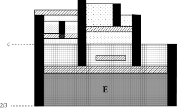
Figure 3. The definition of $\widehat{\mathbf{E}}^{\mathrm{ext}}$. Black rectangles are extended cusp neighbourhoods. The grey transparent region is $\mathbf{E}$. The diagonally lined regions lie outside $\mathbf{M}_{\Gamma}$. The crossed region is $\Sigma\times[2/3,\varsigma]\cap\mathbf{M}_{\Gamma}^{\prime}$. The dotted regions are those that lie outside $\Sigma\times[2/3,\varsigma]$ but need to be added to construct $\widehat{\mathbf{E}}^{\mathrm{ext}}$.

Pulling back the extended brick $\widehat{\mathbf{E}}^{\mathrm{ext}}$ to the sequence $\mathbf{M}_{n}$: Recall that corresponding to the geometric convergence of $\mathbf{M}_{n}$ to $\mathbf{M}_{\Gamma}$, there is an approximate isometry $\mathbf{h}_{n}\colon B_{R_{n}}(\mathbf{M}_{n},\mathbf{x}_{n})\rightarrow B_{K_{n}R_{n}}(\mathbf{M}_{\Gamma},\mathbf{x}_{\infty})$, and that $\mathbf{h}_{n}$ is a $K_{n}$-bi-Lipschitz homeomorphism, where $R_{n}\rightarrow\infty$, $K_{n}\rightarrow 1$, and $\mathbf{x}_{\infty}$ lies on the algebraic locus. We should also recall, as was shown in [Ohs, Lemma 9.2], that the embeddings of $\mathbf{M}_{\Gamma}$ and $\mathbf{M}_{n}$ into $S\times(0,1)$ can be arranged so that the geometric convergence preserves the horizontal levels.

We shall now describe a particular complement $\mathbf{M}_{n}^{\prime}$ of some Margulis tubes in $M_{n}$. Fix a positive constant $\epsilon_{0}$ less than the three-dimensional Margulis constant. Then for large $n$, corresponding to cusp neighbourhoods $U_{l_{1}},\dots,U_{l_{\nu}}$, each $\mathbf{M}_{n}$ has $\epsilon_{0}$-Margulis tubes converging to these cusp neighbourhoods. We define $U^{n}_{l_{k}}$ to be the $\epsilon_{0}$-Margulis tube in $\mathbf{M}_{n}$ corresponding to $U_{l_{k}}$. Then we define $\mathbf{M}_{n}^{\prime}$ to be $\mathbf{M}_{n}\setminus\cup_{k=1}^{\nu}U^{n}_{l_{k}}$. Since there is a homeomorphism between $\mathbf{M}_{n}^{\prime}$ and $\mathbf{M}^{\prime}_{\Gamma}$ preserving the horizontal levels, the union of bricks ${\mathbf{E}}^{\mathrm{br}}$ can be pulled back to a union of bricks in $\mathbf{M}_{n}^{\prime}$, which we define to be $\widehat{\mathbf{E}}_{n}^{\mathrm{ext}}$. We emphasise that $\widehat{\mathbf{E}}_{n}^{\mathrm{ext}}$ is a union of bricks in $\mathbf{M}_{n}^{\prime}$, equipped with the standard brick decomposition, and not in $\mathbf{M}_{n}$. The difference arises precisely from the Margulis tubes $U^{n}_{l_{k}}$.

We take $\epsilon>0$ small enough so that the $\epsilon$-neighbourhoods of $U_{l_{1}},\dots$, which we denote by $U_{l_{1}}(\epsilon),\dots$ respectively, are disjoint. Making $\epsilon$ smaller if necessary, we can assume that, for all $n$, the $\epsilon$-neighbourhoods $U^{n}_{l_{1}}(\epsilon),\dots$ of $U^{n}_{l_{1}},\dots$ are disjoint. Now we define $\mathbf{E}^{\mathrm{ext}}$ to be $\widehat{\mathbf{E}}^{\mathrm{ext}}\setminus\cup_{k=1}^{\nu}U_{l_{k}}(\epsilon)$ and $\mathbf{E}^{\mathrm{ext}}_{n}$ to be $\widehat{\mathbf{E}}_{n}\setminus\cup_{k=1}^{\nu}U^{n}_{l_{k}}(\epsilon)$. Then, by definition, $\{\mathbf{E}^{\mathrm{ext}}_{n}\}$ converges geometrically to $\mathbf{E}^{\mathrm{ext}}$ under the geometric convergence of $\mathbf{M}_{n}$ to $\mathbf{M}_{\Gamma}$. We can define $\mathbf{F}^{\mathrm{ext}}$ and $\mathbf{F}_{n}^{\mathrm{ext}}$ when $\mathbf{F}$ among $\mathbf{F}_{1},\dots,\mathbf{F}_{t}$ is minimal in the same way.

Quasiconvexity of extended bricks $\widehat{\mathbf{E}}^{\mathrm{ext}}$: We shall need the following lemma, which is a generalisation of [DM16, Lemma 2.25].

Lemma 4.4.

Let $\mathbf{E}$ be one of $\mathbf{E}_{1},\dots,\mathbf{E}_{s};\mathbf{F}_{1},\dots,\mathbf{F}_{t}$, and assume that it is minimal. Let $U_{l_{1}},\dots$ be the cusp neighbourhoods associated with $\mathbf{E}$, and suppose that $U_{l_{1}},\dots,U_{l_{\nu}}$ are those specified above. We electrocute $\widetilde{\mathbf{M}}_{\Gamma}$ with respect to the components of the pre-images of $\sqcup_{k=1}^{\nu}U_{l_{k}}$, and obtain a Gromov hyperbolic metric $d^{0}_{\mathbf{M}}$. In the same way, we electrocute $\widetilde{\mathbf{M}}_{n}$ at the components of the preimages of $\sqcup_{k=1}^{\nu}U^{n}_{l_{k}}$. Then, there is a constant $K$ depending only on $\Gamma$ such that each component of the preimage $\widetilde{\mathbf{E}}^{\mathrm{ext}}$ of $\mathbf{E}^{\mathrm{ext}}$ in $(\widetilde{\mathbf{M}}_{\Gamma},d^{0}_{\mathbf{M}})$ and each component of the preimage $\widetilde{\mathbf{E}}^{\mathrm{ext}}_{n}$ of $\mathbf{E}^{\mathrm{ext}}_{n}$ in $(\widetilde{\mathbf{M}}_{n},d^{0}_{n})$ are $K$-quasi-convex.

Proof.

Since $\mathbf{E}^{\mathrm{ext}}$ is the geometric limit of $\mathbf{E}^{\mathrm{ext}}_{n}$ under the geometric convergence of $\mathbf{M}_{n}$ to $\mathbf{M}_{\Gamma}$, it suffices to prove that there exists $K\geq 1$ such that for all $n$, each component of $\widetilde{\mathbf{E}}_{n}^{\mathrm{ext}}$ is $K$-quasi-convex in $\widetilde{\mathbf{M}}_{n}$.

Each horizontal boundary component of $\mathbf{E}^{\mathrm{ext}}_{n}$ corresponds to a horizontal boundary component of $\widehat{\mathbf{E}}^{\mathrm{ext}}$ under $\mathbf{h}_{n}$. Fix a such a horizontal boundary component $F$ of $\widehat{\mathbf{E}}^{\mathrm{ext}}$, and consider the corresponding horizontal boundary component $F^{n}$ of $\mathbf{E}_{n}^{\mathrm{ext}}$ for each $n$. Let $B_{n}$ be the brick in $\mathbf{E}^{\mathrm{ext}}_{n}$ containing $F^{n}$. The geometric limit of $\mathbf{E}^{\mathrm{ext}}_{n}$ with basepoint on $F^{n}$ is a brick in $\mathbf{E}^{\mathrm{ext}}$ containing $F$. We shall only describe the situation in the case when $\mathbf{E}$ is among $\mathbf{E}_{1},\dots,\mathbf{E}_{s}$, and hence $F$ is an upper boundary component. The case when $\mathbf{E}$ is among $\mathbf{F}_{1},\dots,\mathbf{F}_{t}$ and $F$ is a lower boundary component can be dealt with in the same way.

The model manifold $\mathbf{M}_{n}$ contains Margulis tubes which induce a decomposition of $\mathbf{M}_{n}$ into blocks as in Minsky [Min10]. (We are using a slightly non-standard definition of Margulis tube here. We simply fix a constant $\epsilon>0$ and by ‘Margulis tube’, we means a tubular neighbourhood of a closed geodesic whose length is uniformly bounded.) Let $a_{1},\dots,a_{p}$ be core curves of annuli which are the intersection of $F^{n}$ with these Margulis tubes. The lengths of the core curves $a_{1},\dots,a_{p}$ may be greater than the three-dimensional Margulis constant, but are bounded from above by the Bers’ constant depending only the topological type of $S$ [Min10, p. 20]. By taking $\epsilon$ large enough, we can ensure that the curves constitute a pants decomposition of $F^{n}$.

Drilling: We now proceed to drill the Margulis tubes $U^{n}_{l_{1}},\dots,U^{n}_{l_{\nu}}$ of $\mathbf{M}_{n}$, i.e. remove the core geodesics of $U^{n}_{l_{1}},\dots,U^{n}_{l_{\nu}}$ and equip the resulting rank two cusp with a complete hyperbolic metric, while leaving all the end-invariants (ending laminations or conformal structures) of $M_{n}$ unchanged (see [BB04] for details on drilling). Let $M_{n}^{\mathrm{dr}}$ denote the drilled manifold obtained by drilling $M_{n}$.

The drilling theorem of Brock-Bromberg [BB04] shows that there exist positive constants $\delta_{n}$ satisfying the following:

1. $\delta_{n}\to 0$ as $n\to\infty$.

2. $M_{n}$ is $(1+\delta_{n})$-bi-Lipschitz homeomorphic to ${M}_{n}^{\mathrm{dr}}$ away from the Margulis tubes and cusps corresponding to $U^{n}_{l_{1}},\dots,U^{n}_{l_{\nu}}$.

The model manifold ${\mathbf{M}}_{n}^{\mathrm{dr}}$ is a model manifold of the non-cuspidal part of $M_{n}^{\mathrm{dr}}$ and is obtained by replacing the Margulis tubes $U^{n}_{l_{1}},\dots,U^{n}_{l_{\nu}}$ of $\mathbf{M}_{n}$ by their torus boundaries. Topologically, ${\mathbf{M}}_{n}^{\mathrm{dr}}$ is the same as $\mathbf{M}_{n}\setminus\cup_{k=1}^{\nu}U^{n}_{l_{k}}$.

Since the new boundary components of ${\mathbf{M}}_{n}^{\mathrm{dr}}$ are precisely the torus boundaries of $U^{n}_{l_{1}},\dots,U^{n}_{l_{\nu}}$, the brick decomposition of ${\mathbf{M}}_{n}^{\mathrm{dr}}$ can be assumed to coincide with that of $\mathbf{M}_{n}\setminus\cup_{k=1}^{\nu}U^{n}_{l_{k}}$. Recall that $B_{n}$ is the brick in $\mathbf{E}^{\mathrm{ext}}_{n}$ containing $F^{n}$. Thus, there is a brick and a horizontal boundary in ${\mathbf{M}}_{n}^{\mathrm{dr}}$ corresponding to $B_{n}$ and $F^{n}$, which we denote respectively by ${B}_{n}^{\mathrm{dr}}$ and ${F}^{n,\mathrm{dr}}$. It thus suffices to prove the uniform quasi-convexity of ${B}_{n}^{\mathrm{dr}}$.

Quasi-Fuchsian cover of drilled manifold: Recall that $\mathbf{E}\cong\Sigma\times[2/3,5/6)$. Consider the covering $\overline{\mathbf{M}}_{n}$ of ${\mathbf{M}}_{n}^{\mathrm{dr}}$ corresponding to $\pi_{1}(\Sigma)=\pi_{1}({B}_{n}^{\mathrm{dr}})$. Then $\overline{\mathbf{M}}_{n}$ is a (cover corresponding to a) quasi-Fuchsian group of type $\Sigma$, where the boundary components of $\Sigma$ are taken to be parabolics. The shortest pants decomposition of the upper convex core boundary of $\overline{\mathbf{M}}_{n}$ is projected down to ${\mathbf{M}}_{n}^{\mathrm{dr}}$ as a pants decomposition with length bounded independently of $n$. It follows that it is within a uniformly bounded distance from the simplex spanned by $a_{1},\dots,a_{p}$ in the curve complex of $F$. Therefore, if there is no homotopy between the pleated surface realising $a_{1},\dots,a_{p}$ in $\overline{\mathbf{M}}_{n}$ and the upper convex core boundary with uniformly bounded diameter, then there must be a parabolic element in the geometric limit of $\overline{M}_{n}$ which corresponds to a non-peripheral curve of ${F}^{n,\mathrm{dr}}$. This contradicts the assumption that $F$ is an upper boundary component of $\mathbf{E}^{\mathrm{ext}}$ and there is no parabolic curve associated with $\mathbf{E}$ above such a boundary component which is homotopic into $F$. This implies that there does exist such a homotopy with a uniformly bounded diameter (or equivalently, the tracks of points in the homotopy have uniformly bounded diameter).

The lower horizontal boundary component of $\mathbf{E}^{\mathrm{ext}}$, which we denote by $\Sigma_{\Gamma}$, is homeomorphic to $\Sigma$, and if we take the covering of $M_{\Gamma}$ associated with $\pi_{1}(\Sigma)$, this boundary faces a geometrically finite end. This horizontal surface corresponds to the lower boundary component of $\mathbf{E}_{n}^{\mathrm{ext}}$, which we denote by $\Sigma_{n}$ for each $n$. The corresponding lower end of $\overline{M}_{n}$ has a neighbourhood converging geometrically to a neighbourhood of this end. Therefore, by the same argument as above, we see that there is a homotopy between the pleated surface realising the core curve of the Margulis tubes intersecting $\Sigma_{n}$ in $\overline{M}_{n}$ and the lower convex core boundary with a uniformly bounded diameter.

Completing the proof of quasiconvexity, Lemma 4.4: Now, we prove the uniform quasi-convexity of $\widetilde{\mathbf{E}}^{\mathrm{ext}}_{n}$ by contradiction. Suppose that there is a sequence of arcs $a_{n}$ in $\widetilde{\mathbf{E}}^{\mathrm{ext}}_{n}$ such that

1. The geodesic arc $a^{*}_{n}$ is homotopic to $a_{n}$ relative to endpoints.

2. There exists a point $p_{n}$ in $a^{*}_{n}$ whose distance from $\widetilde{\mathbf{E}}^{\mathrm{ext}}_{n}$ with respect to $d^{0}_{n}$ goes to $\infty$ as $n\rightarrow\infty$.

We can assume that $\mathbf{E}_{n}^{\mathrm{ext}}$ and the projection of these arcs $a_{n}$ and $a_{n}^{*}$ into $\mathbf{M}_{n}$ all lie in ${\mathbf{M}}_{n}^{\mathrm{dr}}$ instead of $\mathbf{M}_{n}$ since ${\mathbf{M}}_{n}^{\mathrm{dr}}$ and $\mathbf{M}_{n}$ are uniformly bi-Lipschitz away from cusps and Margulis tubes. We consider the case when $p_{n}$ lies above $\widetilde{\mathbf{E}}^{\mathrm{ext}}_{n}$ with respect to the parametrisation $\widetilde{S}\times(0,1)$, where $\widetilde{S}$ denotes the universal cover of $S$. (When $p_{n}$ lies below $\widetilde{\mathbf{E}}^{\mathrm{ext}}_{n}$, the argument works exactly in the same way by considering $\Sigma$ instead of $F_{1},\dots,F_{1}$ in the argument below.) Let $F_{1},\dots F_{q}$ be the upper horizontal boundary components of $\mathbf{E}^{\mathrm{ext}}_{\Gamma}$, and $F^{n}_{1},\dots,F^{n}_{q}$ the corresponding horizontal boundary components of $\mathbf{E}^{\mathrm{ext}}_{n}$. Then there must be a subarc $b_{n}^{*}$ of the projection of $a_{n}^{*}$ into ${\mathbf{M}}_{n}^{\mathrm{dr}}$ containing the projection $\bar{p}_{n}$ of $p_{n}$, whose endpoints lie on the union of $F^{n}_{1},\dots,F^{n}_{q}$ and $\partial U^{n}_{l_{1}},\dots\partial U^{n}_{l_{\mu}}$ and which is homotopic into $\cup_{k=1}^{q}F^{n}_{k}\cup\cup_{j=1}^{\nu}U^{n}_{l_{j}}(\epsilon)$. (Note that we are now in ${\mathbf{M}}_{n}^{\mathrm{dr}}$, and hence $U^{n}_{l_{1}},\dots,U^{n}_{l_{\nu}}$ are torus cusp neighbourhoods.) See Figure 4.

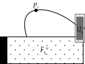
Figure 4. The arc $b^{*}_{n}$ contains the point $p_{n}$, and is homotopic into $\cup_{k=1}^{q}F^{n}_{k}\cup\cup_{j=1}^{\nu}U^{n}_{l_{j}}(\epsilon)$

The distance between $\bar{p}_{n}$ and $\mathbf{E}_{n}^{\mathrm{ext}}$ with respect to $d^{0}_{n}$ goes to $\infty$ by our choice of $p_{n}$. On the other hand, $b_{n}^{*}$ must be contained in a uniformly bounded neighbourhood of the union of the convex cores of $\mathbf{E}_{n}^{\mathrm{ext}}$ and $\cup_{j=1}^{\nu}U^{n}_{l_{j}}$ since $b_{n}^{*}$ must be within a uniformly bounded distance from the corresponding electro-ambient geodesic (see Lemma 2.1) with respect to the electric metric obtained by electrocuting components of the preimages of $\cup_{j=1}^{\nu}U^{n}_{l_{j}}$ in the universal cover $\widetilde{\mathbf{M}}_{n}$. Since there is a homotopy with uniformly bounded diameter between $F^{n}_{k}$ and the corresponding convex core boundary, this is a contradiction. ∎

The induction step: We now explain the induction step mentioned in the outline of the proof of Proposition 4.3 following the statement of Proposition 4.3. This will culminate in Lemma 4.5.

It follows, as was explained in §2.2, that we can electrocute the components of the pre-image $\widetilde{\mathbf{E}}^{\mathrm{ext}}$ of $\mathbf{E}^{\mathrm{ext}}$ in $(\widetilde{\mathbf{M}}_{\Gamma},d_{\mathbf{M}}^{0})$ and get a Gromov hyperbolic (pseudo-)metric on $\widetilde{\mathbf{M}}_{\Gamma}$. We can also electrocute the components of the preimage $\widetilde{\mathbf{E}}_{n}^{\mathrm{ext}}$ of $\mathbf{E}_{n}^{\mathrm{ext}}$ in $(\widetilde{\mathbf{M}}_{n},d_{n}^{0})$ and get a Gromov-hyperbolic space. We denote the new electric metrics by $d^{1}_{\mathbf{M}}$ and $d^{1}_{n}$ respectively, and use $\widetilde{\mathbf{M}}_{\Gamma}^{1}$ and $\widetilde{\mathbf{M}}_{n}^{1}$ as shorthand for $(\widetilde{\mathbf{M}}_{\Gamma},d^{1}_{\mathbf{M}})$ and $(\widetilde{\mathbf{M}}_{n},d^{1}_{n})$. Then $\widetilde{\mathbf{M}}_{n}^{1}$ converges geometrically to $\widetilde{\mathbf{M}}_{\Gamma}^{1}$. In the new metric, geodesic arcs homotopic to subarcs of $r_{\zeta}^{\mathbf{M}}$ going deep into $\widetilde{\mathbf{E}}$ may be conveniently ignored, which is what electrocution allows us to do. However, we need to handle arcs that go deep into the pre-images of the other ends. For this, we need the second electrocution process as follows.

Let $\mathbf{E}^{\prime}$ be one of $\mathbf{E}_{1},\dots,\mathbf{E}_{s};\mathbf{F}_{1},\dots,\mathbf{F}_{t}$ other than the $\mathbf{E}$ we took in Lemma 4.4. We say that $\mathbf{E}^{\prime}=\Sigma^{\prime}\times[2/3,5/6)$ among $\mathbf{E}_{1},\dots,\mathbf{E}_{s}$ is second minimal if there is no $\Sigma_{j}^{\prime}\,(j=1,\dots,t)$ that can be isotoped into $\Sigma$ except for the case when $\mathbf{F}_{j}$ is the $\mathbf{E}$ chosen above. In the same way, we define $\mathbf{E}^{\prime}=\Sigma\times(1/6,1/3]$ among $\mathbf{F}_{1},\dots,\mathbf{F}_{t}$ to be second minimal.

Suppose that $\mathbf{E}^{\prime}$ is second minimal. For simplicity of exposition, we assume that $\mathbf{E}^{\prime}$ is one of $\mathbf{E}_{1},\dots,\mathbf{E}_{s}$. Below we define ${\mathbf{E}^{\prime}}^{\mathrm{ext}}$ and ${\mathbf{E}^{\prime}}_{n}^{\mathrm{ext}}$ in the same way as we defined $\mathbf{E}^{\mathrm{ext}}$ and $\mathbf{E}_{n}^{\mathrm{ext}}$:
By renumbering the $U_{l_{k}}$, let $U_{l_{1}},\dots,U_{l_{w}}$ be the cusp neighbourhoods that abut on $\mathbf{E}^{\prime}$. We consider the brick $\dot{\mathbf{E}}^{\prime}$ in $S\times(0,1)\setminus\cup_{k=1}^{w}U_{l_{k}}$ containing $\mathbf{E}^{\prime}$, let $s^{\prime}$ be $\min\sup_{k=1}^{w}\sup U_{l_{k}}$, and let $U_{l_{w+1}},\dots,U_{l_{x}}$ the cusp neighbourhoods that intersect $\Sigma^{\prime}\times\{s^{\prime}\}$. Then we define $\hat{\mathbf{E}^{\prime}}^{\mathrm{ext}}$ to be the intersection with $\mathbf{M}_{\Gamma}$ of the union of all bricks in $S\times(0,1)\setminus\cup_{k=1}^{x}U_{l_{k}}^{\mathrm{st}}$ that are homotopic into $\Sigma^{\prime}\times[2/3,s^{\prime}]$. By deleting the $\epsilon$-neighbourhoods of $U_{l_{1}},\dots,U_{l_{x}}$, we get ${\mathbf{E}^{\prime}}^{\mathrm{ext}}$. As before, by pulling back ${\mathbf{E}^{\prime}}^{\mathrm{ext}}$ by $\mathbf{h}_{n}$, we get ${\mathbf{E}^{\prime}}^{\mathrm{ext}}_{n}$.

Let $\widetilde{\mathbf{E}^{\prime}}^{\mathrm{ext}}$ and $\widetilde{\mathbf{E}^{\prime}}^{\mathrm{ext}}_{n}$ be the pre-images of ${\mathbf{E}^{\prime}}^{\mathrm{ext}}$ and ${\mathbf{E}^{\prime}}^{\mathrm{ext}}_{n}$ in $\widetilde{\mathbf{M}}_{\Gamma}$ and $\widetilde{\mathbf{M}}_{n}$ respectively. Then by nearly the same argument as in Lemma 4.4, we can show that each component of $\widetilde{\mathbf{E}^{\prime}}^{\mathrm{ext}}$ (resp. $\widetilde{\mathbf{E}^{\prime}}^{\mathrm{ext}}_{n}$) is $K^{\prime}$-quasi-convex in $\widetilde{\mathbf{M}}_{\Gamma}^{1}$ (resp. $\widetilde{\mathbf{M}}_{n}^{1}$) after electrocuting the pre-images of cusp neighbourhoods of those among $U_{l_{1}},\dots,U_{l_{x}}$ (resp. Margulis tubes among $U^{n}_{l_{1}},\dots,U^{n}_{l_{x}}$) that have not been electrocuted in the previous step. Here $K^{\prime}$ is a constant depending only on $\Gamma$.

The part where we need to modify the proof of Lemma 4.4 is the argument to deal with the case when the arc $b^{*}_{n}$ goes out from the lower horizontal boundary $\Sigma_{n}$. In Lemma 4.4 we used the assumption that $\mathbf{E}$ is minimal. In the present setting, it is possible that $\mathbf{E}$ is homotopic into $\mathbf{E}^{\prime}$ in $\mathbf{M}_{\Gamma}$. Still the argument involving the existence of homotopies with uniformly bounded diameters works since we have already electrocuted $\mathbf{E}^{\mathrm{ext}}$ and $\mathbf{E}_{n}^{\mathrm{ext}}$ and we can get homotopies with bounded diameter with respect to electrocuted metrics $d_{n}^{1}$. Therefore (c.f. the discussion in §2.2), we can again electrocute $\widetilde{\mathbf{E}^{\prime}}^{\mathrm{ext}}$ in $(\widetilde{\mathbf{M}}_{\Gamma},d^{1}_{\mathbf{M}})$ and $\widetilde{\mathbf{E}^{\prime}}^{\mathrm{ext}}_{n}$ to get new Gromov hyperbolic metrics denoted by $d^{2}_{\mathbf{M}}$ on $\mathbf{M}_{\Gamma}$ and by $d^{2}_{n}$ on $\mathbf{M}_{n}$ respectively .

We repeat this procedure inductively. Assume that we have defined the electric metrics $d^{m-1}_{\mathbf{M}}$ and $d^{m-1}_{n}$. Then at the next step of induction, we consider an $m$-th minimal $\mathbf{E}$ among $\mathbf{E}_{1},\dots,\mathbf{E}_{s};\mathbf{F}_{1},\dots,\mathbf{F}_{t}$. We construct $\mathbf{E}^{m\mathrm{ext}}$ and $\mathbf{E}^{m\mathrm{ext}}_{n}$ in the same way as we defined $\mathbf{E^{\prime}}^{\mathrm{ext}}$ and ${\mathbf{E}^{\prime}}^{\mathrm{ext}}_{n}$. We define a new electric metric $d^{m}_{\mathbf{M}}$ and $d^{m}_{n}$, by electrocuting the pre-images of $\mathbf{E}^{\mathrm{ext}}$ and ${\mathbf{E}^{\prime}}^{\mathrm{ext}}_{n}$ together with preimages of suitable cusp neighbourhoods or Margulis tubes. The new metrics are again Gromov hyperbolic. Finally, we get hyperbolic electric metrics $d^{s+t}_{\mathbf{M}}$ and $d^{s+t}_{n}$, and denote them by $\bar{d}_{\mathbf{M}}$ and $\bar{d}_{n}$ respectively.

Recall that we have a ray $r_{\zeta}^{\mathbf{M}}:[0,\infty)\rightarrow\widetilde{\mathbf{M}}_{\Gamma}$. For $s_{1},s_{2}\in[0,\infty)$ with $s_{1}<s_{2}$, we denote by $r_{\zeta}^{\mathbf{M}}(s_{1},s_{2})^{*}$ the geodesic arc, parametrised by length, homotopic to $r_{\zeta}^{\mathbf{M}}|[s_{1},s_{2}]$ fixing the endpoints. If we connect $r^{\mathbf{M}}_{\zeta}(s_{1})$ and $r^{\mathbf{M}}_{\zeta}(s_{2})$ by a geodesic arc with respect to $\bar{d}_{\mathbf{M}}$, it fellow-travels $r^{\mathbf{M}}_{\zeta}|[s_{1},s_{2}]$ in $(\widetilde{\mathbf{M}}_{\Gamma},\bar{d}_{\mathbf{M}})$ since all geometrically infinite ends into which the geodesic may escape are electrocuted, along with the cusp neighbourhoods abutting on them. This shows that the electro-ambient quasi-geodesic homotopic to $r_{\zeta}^{\mathbf{M}}|[s_{1},s_{2}]$ fixing the endpoints must pass through the corresponding components of the pre-images of $\mathbf{E}^{\mathrm{ext}}$ for the components of $p^{-1}(\Sigma_{j})\,(j=1,\dots,s)$ and $p^{-1}(\Sigma_{j}^{\prime})\,(j=1,\dots t)$ that $r_{\zeta}([s_{1},s_{2}])$ intersects essentially. Therefore, by Lemma 2.1, we have the following.

Lemma 4.5.

There is a constant $L$ depending only on $\Gamma$ with the following property. Let $\{R_{\alpha}\}_{\alpha}$ be the collection of all components of $p^{-1}(\Sigma_{j})\,(j=1,\dots,s)$ and $p^{-1}(\Sigma_{j}^{\prime})\,(j=1,\dots t)$ that $r_{\zeta}([s_{1},s_{2}])$ intersects essentially (relative to the endpoints). We consider $\mathbf{E}^{\mathrm{ext}}$ for every $\mathbf{E}$ among $\mathbf{E}_{1},\dots,\mathbf{E}_{s};\mathbf{F}_{1},\dots,\mathbf{F}_{t}$, and let $\widetilde{E}_{R_{\alpha}}$ be a component of the pre-image of one of them corresponding to $R_{\alpha}$. Then $r_{\zeta}^{\mathbf{M}}(s_{1},s_{2})^{*}$ is contained in the $L$-neighbourhood of $\cup_{\alpha}\widetilde{E}_{R_{\alpha}}$ with respect to the metric $d_{\mathbf{M}}$.

We also have a $\rho_{n}$-equivariant map $\Phi_{n}\colon{\mathbb{H}}^{2}\rightarrow{\mathbb{H}}^{3}$, and a ray $\Phi_{n}\circ r_{\zeta}$ in ${\mathbb{H}}^{3}$. By pulling back this ray by the lift of the model map $f_{n}$, we get a ray $r^{n}_{\zeta}\colon[0,\infty)\rightarrow\widetilde{\mathbf{M}}_{n}$, where $\widetilde{\mathbf{M}}_{n}$ is the universal cover of $\mathbf{M}_{n}$. For $s_{1}<s_{2}\in[0,\infty)$, we let $r^{n}_{\zeta}(s_{1},s_{2})^{*}$ be the geodesic arc in $\widetilde{\mathbf{M}}_{n}$ connecting $r^{n}_{\zeta}(s_{1})$ and $r^{n}_{\zeta}(s_{2})$. Recall also that each component $R$ of $p^{-1}(\Sigma_{j})$ or $p^{-1}(\Sigma_{j}^{\prime})$ corresponds to a component of the pre-image of $\mathbf{E}_{n}^{\mathrm{ext}}$ for $\mathbf{E}=\mathbf{E}_{j}$ or $\mathbf{E}=\mathbf{F}_{j}$. We denote the component of the preimage of $\mathbf{E}_{n}^{\mathrm{ext}}$ corresponding to $R$ by $\widetilde{E}_{R}^{n}$. Then, using $\mathbf{h}_{n}$ to pull back the components appearing in Lemma 4.5, we get the following.

Lemma 4.6.

There is a constant $L^{\prime}$ independent of $n$ with the following property. Let $\{R_{\alpha}\}_{\alpha}$ be the collection of all components of $p^{-1}(\Sigma_{j})\,(j=1,\dots,s)$ and $p^{-1}(\Sigma_{j}^{\prime})\,(j=1,\dots t)$ that $r_{\zeta}([s_{1},s_{2}])$ intersects essentially (relative to the endpoints) as in Lemma 4.5. Then $r^{n}_{\zeta}(s_{1},s_{2})^{*}$ is contained in the $L^{\prime}$-neighbourhood of $\cup_{\alpha}\widetilde{E}^{n}_{R_{\alpha}}$ with respect to the metric $\bar{d}_{n}$.

Proof of Proposition 4.3:
Since the action of $\pi_{1}(S)$ on ${\mathbb{H}}^{2}$ corresponding to $G$ is properly discontinuous, Assumption 4.1 implies that there is a function $g\colon[0,\infty)\to[0,\infty)$ with $g(x)\to\infty$ as $x\rightarrow\infty$ such that $r_{\zeta}|[s_{1},s_{2}]$ intersects only components of $p^{-1}(\Sigma_{j})$ that are at a distance greater than $g(s_{1})$ from the origin $o_{{\mathbb{H}}^{2}}$. We now fix lifts of the basepoints $\mathbf{o}_{\Gamma}$ in $\widetilde{\mathbf{M}}_{\Gamma}$ and $\mathbf{o}_{n}$ in $\widetilde{\mathbf{M}}_{n}$. These are lifts of $\mathbf{x}_{\infty}$ and $\mathbf{x}_{n}$ respectively. By the IEL assumption of the present Case I and since the electrocution process has been chosen so that two electrocuted pieces are separated by a minimum distance $\epsilon>0$, we see that there is a function $k_{\Gamma}\colon[0,\infty)\rightarrow[0,\infty)$ with $k_{\Gamma}(x)\to\infty$ as $x\to\infty$ such that if $R$ is a component of $p^{-1}(\Sigma_{j})$ that $r_{\zeta}|[s_{1},s_{2}]$ intersects, then $\widetilde{E}_{R}$ is at a distance greater than $k_{\Gamma}(s_{1})$ from $\mathbf{o}_{\Gamma}$. By pulling this back by $\mathbf{h}_{n}$ for large $n$, we see that there is a function $k:[0,\infty)\rightarrow[0,\infty)$ with $k\to\infty$ as $x\to\infty$ such that if $R$ is a component of $p^{-1}(\Sigma_{j})$ that $r_{\zeta}|[s_{1},s_{2}]$ intersects, then $\widetilde{E}^{n}_{R}$ is at the $\bar{d}_{n}$-distance greater than $k(s_{1})$ from $\mathbf{o}_{n}$. By Lemma 4.6, this implies that any point of the geodesic arc $r_{n}(s_{1},s_{2})^{*}$ is at a distance greater than $k(s_{1})-L^{\prime}$ from $\mathbf{o}_{n}$. Since $f_{n}\colon\mathbf{M}_{n}\to{\mathbb{H}}^{3}/G_{n}$ is a bi-Lipschitz map whose Lipschitz constant can be chosen independently of $n$, this concludes the proof of Proposition 4.3. $\Box$

4.2. Case II: $\bar{r}_{\zeta}$ is eventually contained in one subsurface

Now, we turn to Case II, i.e. we suppose that Assumption 4.1 does not hold. Then eventually $r_{\zeta}(t)$ stays in one component $R$ of $p^{-1}(\Sigma_{j})$ or $p^{-1}(\Sigma^{\prime}_{j})$ or $p^{-1}(T_{j})$ or $p^{-1}(T_{j}^{\prime})$. We now assume that $R$ is a component of $p^{-1}(\Sigma_{j})$. We can argue in the same way also for the case when $R$ is a component of $p^{-1}(\Sigma_{j}^{\prime})$ just turning $\mathbf{M}_{\Gamma}$ upside down, whereas for the case when $R$ is a component of $p^{-1}(T_{j})$ or $p^{-1}(T_{j}^{\prime})$ we need a little modification of the argument, which we shall mention at the end of this subsection. We can also assume that if $r_{\zeta}(t)$ is also eventually contained in a component of $p^{-1}(\Sigma^{\prime}_{k})$, then $\Sigma^{\prime}_{k}$ is not contained in $\Sigma_{j}$ up to isotopy, by choosing a minimal element among components containing $r_{\zeta}(t)$ eventually.

4.2.1. Case II A: when $\zeta$ is an endpoint of a lift of a boundary parabolic curve.

We first consider the special case when $\zeta$ is an endpoint of a lift $\tilde{c}$ of a component $c$ of $\operatorname{Fr}\Sigma_{j}$. Then $c_{\infty}(\zeta)$ is a parabolic fixed point of $\rho_{\infty}(\gamma_{c})$, where $\gamma_{c}$ is an element of $G$ corresponding to $c$. We consider the geodesic axis $a_{c}$ of $\rho_{n}(\gamma_{c})$, and let $\mathcal{N}_{n}$ be a neighbourhood in ${\mathbb{H}}^{3}$ given by a lift of the $\epsilon_{0}$-Margulis around the projection of $a_{c}$ to $M_{n}$ for large $n$. Correspondingly, there is a horoball $\mathcal{N}_{\infty}$ stabilised by $\rho_{\infty}(\gamma_{c})$ to which $(\mathcal{N}_{n})$ converges geometrically. Since there is an upper bound for the distance from $\mathcal{N}_{\infty}$ to any point on $\Phi_{\infty}\circ\tilde{c}$, and hence $\Phi_{\infty}\circ r_{\zeta}$, there is an upper bound independent of $n$ for the distance from any point on the image of $\Phi_{n}\circ r_{\zeta}$ to $\mathcal{N}_{n}$.

We define a broken geodesic arc $r_{n}^{+}(s_{1},s_{2})$ consisting of three geodesic arcs as follows. Let $\delta_{s_{1}}^{n}$ and $\delta_{s_{2}}^{n}$ be the shortest geodesic arcs that connect $\Phi_{n}\circ r_{\zeta}(s_{1})$ and $\Phi_{n}\circ r_{\zeta}(s_{2})$ respectively with $\mathcal{N}_{n}$. Let $\delta_{s_{1},s_{2}}^{n}$ be the geodesic arc in $\mathcal{N}_{n}$ connecting the endpoint of $\delta_{s_{1}}$ on $\operatorname{Fr}\mathcal{N}_{n}$ with that of $\delta_{s_{2}}$. We define $r_{n}^{+}(s_{1},s_{2})$ to be the concatenation $\delta^{n}_{s_{1}}*\delta^{n}_{s_{1},s_{2}}*\delta^{n}_{s_{2}}$. Then the observation in the previous paragraph implies that $r_{n}^{+}(s_{1},s_{2})$ is a uniform quasi-geodesic, i.e., there are constants $A,B$ independent of $s_{1},s_{2}$ and $n$ such that $r_{n}^{+}(s_{1},s_{2})$ is an $(A,B)$-quasi-geodesic.

Now, by the convexity of Margulis tubes and the properness of $\Phi_{n}\circ r_{\zeta}$, it is easy to check that there is a function $g^{+}\colon[0,\infty)\to[0,\infty)$ with $g^{+}(u)\to\infty$ as $u\to\infty$ such that any point in $r_{n}^{+}(s_{1},s_{2})$ lies outside the $g^{+}(s_{1})$-ball centred at $o_{{\mathbb{H}}^{3}}$. Since $r_{n}^{+}(s_{1},s_{2})$ is uniformly quasi-geodesic, the geodesic arc connecting $\Phi_{n}\circ r_{\zeta}(s_{1})$ with $\Phi_{n}\circ r_{\zeta}(s_{2})$ is contained in a uniform neighbourhood of $r_{n}^{+}(s_{1},s_{2})$. This shows the EPP condition for $r_{\zeta}$.

4.2.2. Case II B: when $\zeta$ is neither an endpoint of the lift of a boundary parabolic curve nor a crown-tip

Now, we assume that $\zeta$ is neither an endpoint of a lift of a component of $\operatorname{Fr}\Sigma_{j}$ nor a crown-tip. Note that the latter is the standing assumption of this section.

Let $G^{j}$ be a subgroup of $G=\pi_{1}(S)$ corresponding to $\pi_{1}(\Sigma_{j})$, and define $G_{\infty}^{j}$ to be $\rho_{\infty}(G^{j})$. The non-cuspidal part of the hyperbolic 3-manifold ${\mathbb{H}}^{3}/G^{j}_{\infty}$ has a geometrically infinite end $e$ with a neighbourhood homeomorphic to $\Sigma_{j}\times(0,\infty)$.

The proof splits further into subcases.

Subcase II B (i):
We first prove the EPP condition for the following special (sub)case. We say that the geodesic realisation of a geodesic (finite or infinite) in (the intrinsic metric on) $\widetilde{S}(\subset\widetilde{\mathbf{M_{\Gamma}}})$ (resp. ${S}(\subset{\mathbf{M_{\Gamma}}})$) is the geodesic in $\widetilde{\mathbf{M_{\Gamma}}}$ (resp. ${\mathbf{M_{\Gamma}}}$) joining its end points and path-homotopic to it.

Lemma 4.7.

Suppose that there exists a $\Sigma_{k}^{\prime}$ contained in $\Sigma_{j}$ (up to isotopy) and let $\mathbf{F_{k}}$ be the end corresponding to it. If the geodesic realisation $r_{\zeta}^{\mathbf{M}}$ in $\mathbf{M_{\Gamma}}$ is not eventually disjoint from $\mathbf{F_{k}}$, then the EPP condition holds.

Proof.

By our choice of $\Sigma_{j}$, it is impossible that the geodesic realisation of $r^{\mathbf{M}}_{\zeta}$ is eventually contained in one component of the pre-image of $\mathbf{F_{k}}$ in $\widetilde{\mathbf{M}}_{\Gamma}$, as this would imply that $p\circ r_{\zeta}$ is eventually contained in $\Sigma_{k}^{\prime}$ contradicting our choice of $\Sigma_{j}$. Therefore the only possibility under the hypothesis is that $r_{\zeta}^{\mathbf{M}}$ intersects infinitely many components of the pre-image of $\mathbf{F_{k}}$. Then the argument in Section 4.1 goes through to show the EPP condition. ∎

Subcase II B (ii):
Next we consider the subcase when there exists a $T^{\prime}_{k}$ (among $T_{1}^{\prime},\dots,T^{\prime}_{v}$) contained in $\Sigma_{j}$ and $p\circ r_{\zeta}$ is not eventually disjoint from $T_{k}^{\prime}$.

Lemma 4.8.

Suppose that there is a $T_{k}^{\prime}$ contained in $\Sigma_{j}$ up to isotopy. Let $U_{1},\dots,U_{q}$ be the cusps abutting on the geometrically finite end of $({\mathbb{H}}^{3}/\Gamma)_{0}$ corresponding to $T_{k}^{\prime}$. If the geodesic realisation of the ray $r_{\zeta}^{\Gamma}$ is not eventually disjoint from the pre-images of $U_{1}\cup\dots\cup U_{q}$, then the EPP condition holds.

Proof.

Under this assumption, the geodesic realisation of $r_{\zeta}^{\Gamma}$ intersects infinitely many horoballs that are lifts of $U_{1},\dots,U_{q}$ since we are assuming that $\zeta$ is not an endpoint of a lift of a parabolic curve and hence that it is not eventually contained in one among the preimages of $U_{1},\dots,U_{q}$. (Further, since $\zeta$ is not a crown-tip, it cannot be identified with the base-point of such a horoball either.)

We can assume that the same holds for the geodesic realisation of $r_{\zeta}^{\mathbf{M}}$ in the universal cover of the model manifold. (We can properly homotope the ray through a bounded distance if necessary.)

By the approximate isometry $\mathbf{h}_{n}$, these cusps correspond to Margulis tubes $U^{n}_{1},\dots,U_{q}^{n}$. In this situation, we can electrocute $\widetilde{\mathbf{M}}_{\Gamma}$ at the pre-images of $U_{1},\dots,U_{q}$ and $\widetilde{\mathbf{E}}^{\mathrm{ext}}$ together with the pre-images of the cusp neighbourhoods $U_{l_{1}},\dots,U_{l_{\nu}}$ defined in Case 4.1, where $\mathbf{E}$ is defined to be the brick $\mathbf{E}_{j}$. In $\widetilde{\mathbf{M}}_{n}$, we electrocute

1. pre-images of the Margulis tubes $U^{n}_{1},\dots,U_{q}^{n}$,

2. $\mathbf{E}^{\mathrm{ext}}_{n}$ and pre-images of Margulis tubes $U^{n}_{l_{1}},\dots,U^{n}_{l_{\nu}}$.

Then by repeating the argument in Case 4.1, the EPP condition follows. ∎

Subcase II B (iii):
Next we consider the (sub)case when there exists a $\Sigma^{\prime}_{k}$ contained in $\Sigma_{j}$ up to isotopy, but $p\circ r_{\zeta}$ is eventually disjoint from $\Sigma_{k}^{\prime}$, and also there is no $T_{k}^{\prime}$ as in Lemma 4.8.

Lemma 4.9.

Suppose that there exists at least one $\Sigma_{k}^{\prime}$ contained in $\Sigma_{j}$ up to isotopy. Suppose that $p\circ r_{\zeta}$ is eventually disjoint from any $\Sigma_{k}^{\prime}$ that is contained in $\Sigma_{j}$, and that moreover it is not in the situation of Lemma 4.8. Then, there are constants $R$ and $t_{0}$ independent of $n$ such that for all $s_{1},s_{2}\in[0,\infty)$, both greater than $t_{0}$, the geodesic arc $r_{n}(s_{1},s_{2})^{*}$ is contained in the $R$-neighbourhood of $\Phi_{n}(\mathbb{H}^{2})$.

Proof.

Since $p\circ r_{\zeta}$ is eventually disjoint from any $\Sigma_{k}^{\prime}$, there is $t_{0}$ such that $r_{\zeta}(t)$ is contained in a component $F$ of $\Sigma_{j}\setminus(\cup_{k}\Sigma^{\prime}_{k})$ if $t\geq t_{0}$. Let $G^{F}$ be a subgroup of $G$ corresponding to $\pi_{1}(F)$. Let $G_{n}^{F},G_{\infty}^{F}$ be the corresponding subgroups of $G_{n}$ and $G_{\infty}$ respectively. Let $\Gamma_{F}$ be the geometric limit of $(G_{n}^{F})$. Then by the covering theorem [Thu80, Can96, Ohs92], we see that $G^{F}_{\infty}$ is geometrically finite. Further, the only parabolics are those represented by the components of $\operatorname{Fr}\Sigma_{k}^{\prime}$ and those of $\operatorname{Fr}T_{l}^{\prime}$. Since $\Phi_{n}\circ r_{\zeta}$ converges to $r_{\zeta}^{\Gamma}$ under the geometric convergence of $G_{n}$ to $\Gamma$, we can assume that by taking larger $t_{0}$ if necessary, $\Phi_{n}\circ r_{\zeta}(t)$ is contained in the $\epsilon$-neighbourhood of the convex hull of the limit set of $G_{n}^{F}$ for $t\geq t_{0}$. Furthermore, since we are not in the situation of Lemma 4.8, the geodesic realisation of $r_{\zeta}^{\Gamma}$ is eventually disjoint from the horoballs corresponding to parabolic curves lying on $\operatorname{Fr}T_{l}$. This implies that there is a constant $\delta$ such that the geodesic realisation of $r_{\zeta}^{\Gamma}$ is within a bounded distance of the image $q\circ\Phi_{\infty}({\mathbb{H}}^{2})$. Since $\Phi_{n}({\mathbb{H}}^{2})$ converges geometrically to $q\circ\Phi_{\infty}({\mathbb{H}}^{2})$, the geodesic arc connecting two points of $\Phi_{n}\circ r_{\zeta}(s_{1})$ and $\Phi_{n}\circ r_{\zeta}(s_{2})$ with $s_{1},s_{2}\geq t_{0}$ is also within uniformly bounded distance from $\Phi_{n}({\mathbb{H}}^{2})$. ∎

The EPP condition in the situation of Lemma 4.9 is now a replica of the proof of Theorems A, B in [MS13] as we are essentially reduced to the geometrically finite case.

Subcase II B (iv):
We have now come to the remaining subcase. In the discussion so far, we have already dealt with all the cases when the geodesic realisation of $p_{\mathbf{M}}\circ r^{\mathbf{M}}_{\zeta}$ in $\mathbf{M}_{\Gamma}$ can escape farther and farther from $\mathbf{E}$, where $p_{\mathbf{M}}\colon\widetilde{\mathbf{M}}_{\Gamma}\to\mathbf{M}_{\Gamma}$ is the universal covering. Therefore, we can assume that the geodesic realisation of $p_{\mathbf{M}}\circ r^{\mathbf{M}}_{\zeta}$ in $\mathbf{M}_{\Gamma}$ is eventually contained inside a fixed simply degenerate brick $\mathbf{E}$ of $\mathbf{M}_{\Gamma}$.

We assume that $\mathbf{E}$ corresponds to $\Sigma_{j}$. The case when it corresponds to $\Sigma^{\prime}_{k}$ can also be dealt with in the same way. We can then, by moving basepoints, assume that $r_{\zeta}$ is entirely contained in $\Sigma_{j}$. Let $G^{j}$ be the subgroup of $\pi_{1}(S)$ associated with $\pi_{1}(\Sigma_{j})$. We shall use $G_{n}^{j},G_{\infty}^{j}$ respectively for $\rho_{n}(G^{j}),\rho_{\infty}(G^{j})$. Let $\Gamma^{j}$ be a geometric limit of (a subsequence of) $(G_{n}^{j})_{n\in\mathbb{N}}$. Then $\Gamma^{j}$ can be regarded as a subgroup of $\Gamma$.

The geometric limit $\Gamma^{j}$ may be larger than $G_{\infty}^{j}$, but by the covering theorem (see [Can96] and [Ohs92]), there is a neighbourhood $\bar{E}_{j}$ of $\bar{e}_{j}$, that projects homeomorphically to a neighbourhood $\hat{E}_{j}$ of a geometrically infinite end of $({\mathbb{H}}^{3}/\Gamma^{j})_{0}$. Renumbering the parabolic curves on $S$, we assume that $c_{1},\dots,c_{p}$ are the parabolic curves on $\Sigma_{j}$ including those corresponding to components of $\operatorname{Fr}\Sigma_{j}$. Each $c_{k}$ corresponds to either a $\mathbb{Z}$-cusp or a $\mathbb{Z}\times\mathbb{Z}$-cusp in ${\mathbb{H}}^{3}/\Gamma^{j}$. Let $U_{k}$ denote a neighbourhood of $c_{k}$. Recall that by the geometric convergence of ${\mathbb{H}}^{3}/G_{n}^{j}$ to ${\mathbb{H}}^{3}/\Gamma^{j}$, these cusp neighbourhoods correspond to Margulis tubes in ${\mathbb{H}}^{3}/G^{j}_{n}$ for large $n$. We denote the corresponding Margulis tubes in ${\mathbb{H}}^{3}/G_{n}^{j}$ by $U^{n}_{1},\dots,U^{n}_{p}$.

We now electrocute $U_{1},\dots,U_{p}$ in ${\mathbb{H}}^{3}/\Gamma^{j}$ to get a new metric $\bar{d}_{\Gamma^{j}}$, and accordingly we electrocute $U^{n}_{1},\dots,U^{n}_{p}$ in ${\mathbb{H}}^{3}/G_{n}^{j}$ to get a new metric $\bar{d}_{n}$ in such a way that $({\mathbb{H}}^{3}/G_{n}^{j},\bar{d}_{n})$ converges geometrically to $({\mathbb{H}}^{3}/\Gamma^{j},\bar{d}_{\Gamma^{j}})$. Let $r_{\zeta}^{\Gamma}(s_{1},s_{2})^{*}$ be the geodesic arc in ${\mathbb{H}}^{3}$ connecting $r_{\zeta}^{\Gamma}(s_{1})$ with $r_{\zeta}^{\Gamma}(s_{2})$. Also, let $r_{\zeta}^{\Gamma}(s_{1},s_{2})^{\times}$ be the geodesic arc with respect to the electric metric $\bar{d}_{\Gamma^{j}}$. As per our previous terminology, $r_{\zeta}^{\Gamma}(s_{1},s_{2})^{*}$ is the geodesic realisation of $r_{\zeta}^{\Gamma}([s_{1},s_{2}])$. The hypothesis of Subcase II B (iv) can then be restated as follows:

Assumption 4.10.

There is a constant $R^{\prime}$ such that for any $s_{1},s_{2}\in[0,\infty)$, the geodesic realisation $r_{\zeta}^{\Gamma}(s_{1},s_{2})^{*}$ is contained in the $R^{\prime}$-neighbourhood of $\hat{E}_{j}$ with respect to the (electric) metric $\bar{d}_{\Gamma}$.

Under Assumption 4.10, we are reduced to the case where the geodesic realisations $r_{\zeta}^{\Gamma}(s_{1},s_{2})^{*}$ can only go deep into the end $\bar{e}^{j}$. This is exactly the situation dealt with in [Mj14a, Corollary 6.13] or in the proof of [MS17, Theorem A] in Section 4.2.3 of that paper:
We approximate the geodesics $r_{\zeta}^{\Gamma}(s_{1},s_{2})^{*}$ or $r_{\zeta}^{\Gamma}(s_{1},s_{2})^{\times}$ by quasi-geodesics using the construction of model manifolds. Geometric convergence to the end $\mathbf{E}$ of the approximants $\mathbf{E}^{n}$ ensures the geometric convergence of their model manifolds. Corollary 6.13 [Mj14a] now translates to the EPP condition as in the proof of [MS17, Theorem A].

4.2.3. The case when $p\circ r_{\zeta}$ is eventually contained in a geometrically finite $T_{j}$

Recall that $T_{j}$ corresponds to a geometrically finite end. This case is simpler than previous one and we can repeat most of the arguments of the previous cases. If $\zeta$ is an endpoint of a lift of a parabolic curve, the argument in Case II A goes through without modification as we did not use the assumption that $\Sigma_{j}$ corresponds to a simply degenerate end there. For the analogues of Cases II B-(i, ii, iii) too we can argue in the same way as there to show the EPP condition.

In the remaining case, since the end $e$ corresponding to $T_{j}$ is geometrically finite, the geodesic realisation of $r_{\zeta}^{\Gamma}$ cannot escape towards $e$, as in the case of simply degenerate end. Therefore the only possibility is that it lies in a neighbourhood of $q\circ\Phi_{\infty}({\mathbb{H}}^{2})$. Thus, this is the same situation as Case II B (iii).

5. Pointwise convergence for tips of crown domains

We shall now prove what remains in order to complete the proofs of Theorems 2.16 and 2.17:
If $\zeta$ is a tip of a crown domain $C$ for $(\lambda,\sigma)$, where $\sigma$ is a parabolic curve and $\lambda$ is an ending lamination, and either the cusp corresponding to $\sigma$ is not conjoining, or $e$ is not coupled, or $\sigma$ is twisted, or $C$ is not well approximated, then the Cannon-Thurston maps do converge at $\zeta$.

The proof splits into three cases:

1. Either the cusp corresponding to $\sigma$ is not conjoining or $e$ is not coupled. This case will be dealt with in Proposition 5.1 below, and for a special case in Proposition 5.2.

2. $e$ is coupled but the crown domain $C$ is not well approximated. This will be dealt with in Proposition 5.2 below.

3. The cusp corresponding to $\sigma$ is twisted. This will be dealt with in Proposition 5.3 below.

Now we consider the case when either the cusp corresponding to $\sigma$ is not conjoining or $e$ is a simply degenerate end that is not coupled. We shall consider the point-wise convergence of Cannon-Thurston maps at crown-tips $(\lambda,\sigma)$. Without loss of generality, we assume that $e$ is upward as usual. Let $U$ be a $\mathbb{Z}$-cusp neighbourhood of ${\mathbb{H}}^{3}/\Gamma$ corresponding to $\sigma$. Let $A$ be an open annulus bounding $U$. Let $e^{\prime}$ be another end on which $U$ abuts. By assumption, $e^{\prime}$ is not coupled with $e$. Then

1. Either $e^{\prime}$ is also an upward algebraic end (if $U$ is not conjoining this is the only case), or

2. $e^{\prime}$ is downward, but by taking the approximate isometry $h_{n}^{-1}$, a neighbourhood of $e^{\prime}$ does not contain a surface $\Sigma^{\prime}_{+}$ as in (3)-(c) of Definition 2.11 which is parallel into a neighbourhood of $e$.

The proof of the case (b) is deferred and will be dealt with in Proposition 5.2 together with the case when the crown domain $C$ is not well approximated.

We now state the point-wise continuity in the case (a) above.

Proposition 5.1.

Let $e$ be a simply degenerate end of $({\mathbb{H}}^{3}/G_{\infty})_{0}$ corresponding to a subsurface $\Sigma$ of $S$, and let $\sigma$ be a component of $\operatorname{Fr}\Sigma$. Suppose that either $e$ is not coupled or the cusp $U$ of ${\mathbb{H}}^{3}/\Gamma$ corresponding to $\sigma$ is not conjoining. In the former case, we assume moreover that condition (a) above holds. Let $\lambda$ be the ending lamination for $e$, whose minimal supporting surface is $\Sigma$. Let $\zeta$ be a crown-tip of $(\sigma,\lambda)$. Also, let $c_{n}\,(n=1,\cdots,\infty)$ denote the Cannon-Thurston maps for the representations $\rho_{n}\,(n=1,\cdots,\infty)$. Then we have $c_{n}(\zeta)\to c_{\infty}(\zeta)$.

Proof.

The cusp $U$ corresponds to a Margulis tube $U^{n}$ in ${\mathbb{H}}^{3}/G_{n}$ under the approximate isometry $h_{n}^{-1}$ for large $n$. The core curve of $U^{n}$ is freely homotopic to $\rho_{n}(\sigma)$. We denote by $\mathbf{U}$ and $\mathbf{U}^{n}$ their counterparts in the model manifolds $\mathbf{M}_{\Gamma}$ and $\mathbf{M}_{n}$. In the model manifold $\mathbf{M}_{n}$, the Margulis tube $\mathbf{U}^{n}$ is bounded by a torus $\mathbf{T}_{n}$ consisting of two horizontal annuli and two vertical annuli. These in turn correspond to the boundary $T_{n}$ of $U^{n}$. Let $A_{l}^{n},A_{r}^{n}$ be the two vertical annuli in $\mathbf{T}_{n}$, thought of as the left and right vertical annulus respectively. Under condition (a), $\mathbf{T}_{n}$ converges to neither a torus nor a conjoining annulus. Therefore, we see that the moduli of both $A_{l}^{n}$ and $A_{r}^{n}$ go to $\infty$ as $n\to\infty$. Let $\mathbf{E}$ be the brick of $\mathbf{M}_{\Gamma}^{0}$ containing the end $f_{\Gamma}^{-1}(e)$. We denote by $\mathcal{U}$ the union of cusp neighbourhoods of $\mathbf{M}_{\Gamma}$ abutting on $e$, and by $\mathcal{U}^{n}$ the union of Margulis tubes corresponding to $\mathcal{U}$ under the approximate isometry $\mathbf{h}_{n}$. Then, if we regard $\mathbf{M}_{n}\setminus\mathcal{U}^{n}$ as a brick manifold with bricks consisting of maximal sets of parallel horizontal surfaces, there is a brick $\mathbf{E}_{n}$ of $\mathbf{M}_{n}\setminus\mathcal{U}^{n}$ which corresponds to $\mathbf{E}$ under $\mathbf{h}_{n}$. Since $T_{n}$ converges to $A$ geometrically, we see that $\mathbf{E}_{n}$ converges geometrically to $\mathbf{E}$ whenever we choose a basepoint within a bounded distance from the algebraic locus. We denote the counterpart of $\mathbf{E}_{n}$ and $\mathbf{E}$ in ${\mathbb{H}}^{3}/G_{n}$ and ${\mathbb{H}}^{3}/\Gamma$ by $E_{n}$ and $E$ respectively.

Now consider a pleated surface $f_{n}\colon S\to{\mathbb{H}}^{3}/G_{n}$ realising $\lambda$ and inducing $\rho_{n}$ between the fundamental groups. Let $\tilde{f}_{n}\colon{\mathbb{H}}^{2}\to{\mathbb{H}}^{3}$ be its lift. The endpoint at infinity $c_{n}(\zeta)$ is also an endpoint at infinity of a leaf $\ell_{n}$ of the pleating locus of $\tilde{f}_{n}$. It is in fact a lift of a leaf of $\lambda_{C}$. Therefore, the geodesic realisation $r_{\zeta}^{n}$ of $\Phi_{n}\circ r_{\zeta}$ (setting its starting point to be $o_{{\mathbb{H}}^{3}}$) is asymptotic to this leaf $\ell_{n}$. Next note that $(E_{n})$ converges geometrically to $E$. Further, $\lambda_{C}$, which consists of leaves of $\lambda$, is not realisable in $E$. Hence, for any compact set $K$, there exists $n_{0}$ such that for $n\geq n_{0}$, the surface $f_{n}(S)\cap E_{n}$ is disjoint from $h_{n}^{-1}(K)$. Let $\widetilde{U}$ be a lift of $U$ corresponding to a lift of $\sigma$ lying on the boundary of the crown domain $C$ having $\zeta$ as a vertex. Then $\widetilde{U}$ is a horoball touching $S^{2}_{\infty}$ at $c_{\infty}(\zeta)$. The geodesic ray $r_{\zeta}^{n}$ can then be properly homotoped to a quasi-geodesic ray $\bar{r}_{\zeta}^{n}$ consisting of two geodesics; one connecting $o_{{\mathbb{H}}^{3}}$ to the point $z_{n}$ on $\ell_{n}$ nearest to $\widetilde{U}$, and a geodesic ray connecting $z_{n}$ to $c_{n}(\zeta)$ lying in the image of $\tilde{f}_{n}$. Since the moduli of both $A_{l}^{n}$ and $A_{r}^{n}$ go to $\infty$, the exterior angle of the two constituents of $\bar{r}_{\zeta}^{n}$ is bounded away from $\pi$. Hence $(\bar{r}_{\zeta}^{n})$ is uniformly quasi-geodesic. Since the time $\bar{r}_{\zeta}^{n}$ spends in $U^{n}$ goes to $\infty$, the same holds for $r_{\zeta}^{n}$. Finally note that $U^{n}$ converges to $U$ and the latter lifts to a horoball $\widetilde{U}$ touching $S^{2}_{\infty}$ at only one point $c_{\infty}(\zeta)$. Hence $(c_{n}(\zeta))$ converges to $c_{\infty}(\zeta)$. ∎

Now we consider the second case when $P$ is conjoining but $e$ is not coupled or $C$ is not well approximated.

Proposition 5.2.

Let $e$ be a simply degenerate end of $({\mathbb{H}}^{3}/G_{\infty})_{0}$ corresponding to the subsurface $\Sigma$ of $S$. Let $\lambda$ be the ending lamination for $e$ supported on $\Sigma$ and $\sigma$ a parabolic curve whose corresponding cusp abuts on $e$. Suppose that

1. Either $e$ is not coupled and the condition (b) before Proposition 5.1 holds,

2. Or, a crown domain $C$ for $(\lambda,\sigma)$ is not well approximated.

Let $\zeta$ be a tip of $C$. Also, let $c_{n}\,(n=1,\cdots,\infty)$ denote the Cannon-Thurston maps for the representations $\rho_{n}\,(n=1,\cdots,\infty)$. Then $(c_{n}(\zeta))$ converges to $c_{\infty}(\zeta)$.

Proof.

We retain the notation in the proof of Proposition 5.1 and assume that $e$ is upward. We take a pleated surface $f_{n}\colon S\to{\mathbb{H}}^{3}/G_{n}$ realising $\lambda\cup\operatorname{Fr}\Sigma$. Since the pleated surface $f_{n}$ realises $\lambda$, it follows that if $(f_{n}|\Sigma)$ converges geometrically, then after passing to a subsequence, we obtain a pleated surface map from $\Sigma$ to ${\mathbb{H}}^{3}/\Gamma$. This implies, however, that $e$ is coupled and $C$ is well approximated, contradicting the assumption. Therefore, $(f_{n})$ cannot converge geometrically.

Let $m_{n}$ be the hyperbolic structure on $\Sigma$ induced from ${\mathbb{H}}^{3}/G_{n}$ by $f_{n}$. If $(m_{n})$ is bounded in the moduli space then by the compactness of unmarked pleated surfaces, $(f_{n})$ must converge geometrically (after passing to a subsequence) as above. Therefore $(m_{n})$ is unbounded. Hence there is an essential simple closed curve $s_{n}$ in $\Sigma$ such that $\operatorname{length}_{m_{n}}(s_{n})\to 0$. We can choose $s_{n}$ so that for a component $W_{n}$ of $\Sigma\setminus s_{n}$ containing $\sigma$ in its boundary, $(W_{n},m_{n})$ converges geometrically to a complete hyperbolic surface. If there is a limiting pleated surface realising $\lambda_{C}$ in the partner(s) of $e$, then $e$ is coupled and $C$ is well approximated, contradicting our assumption.

It follows that the only possibility is that the distance from the basepoint and $f_{n}(\Sigma)$ goes to $\infty$. By repeating the argument in the proof of Proposition 5.1, we see that $(c_{n}(\zeta))$ converges to $c_{\infty}(\zeta)$. ∎

Now we turn to the last case when the cusp $P$ is twisted although the end is coupled, $P$ is conjoining, and $C$ is well approximated.

Proposition 5.3.

Let $e$ be a coupled simply degenerate end of $({\mathbb{H}}^{3}/G_{\infty})_{0}$ corresponding to the subsurface $\Sigma$ of $S$. Let $\lambda$ be the ending lamination for $E$ supported on $\Sigma$ and let $\sigma$ be a parabolic curve corresponding to a twisted cusp $P$ abutting on $e$. Let $\zeta$ be a tip of a crown domain $C$ of $(\lambda,c)$. We assume that $C$ is well approximated. Let $c_{n}\,(n=1,\cdots,\infty)$ denote the Cannon-Thurston maps for the representations $\rho_{n}$, $n=1,\cdots,\infty$. Then $(c_{n}(\zeta))$ converges to $c_{\infty}(\zeta)$.

Proof.

We shall use notation from §3. In particular, we consider a leaf $\ell$ of the pre-image of $\lambda$ in ${\mathbb{H}}^{2}$, whose endpoint at infinity is $\zeta$. The only difference from the situation in §3 is that the cusp $P$ is twisted now. As in §3, we consider the realisation $\tilde{\ell}_{n}$ of $\ell$ and an arc $a^{n}_{\ell}$ in ${\mathbb{H}}^{3}$ connecting $o_{{\mathbb{H}}^{3}}$ to $\tilde{\ell}_{n}$ that bridges over $\widetilde{P}^{n}$. Then, since $P$ is twisted, the landing point $y_{n}$ of $a^{n}_{\ell}$ has distance from $o_{{\mathbb{H}}^{3}}$ going to $\infty$, and the time it spends in a lift $\widetilde{P}^{n}$ of the Margulis tube $P^{n}$ also goes to $\infty$. Recall that $\widetilde{P}^{n}$ converges to a horoball $\widetilde{P}$ touching $S^{2}_{\infty}$ at $c_{\infty}(\zeta)$. This shows that $c_{n}(\zeta)$, which is the endpoint at infinity of $\ell$, converges to $c_{\infty}(\zeta)$. ∎

References

- [Bow12] B. H. Bowditch. Relatively hyperbolic groups. Internat. J. Algebra and Computation. 22, 1250016, 66pp, 2012.
- [Bro01] J. Brock. Iteration of mapping classes and limits of hyperbolic 3-manifolds. Invent. Math. 143 no 3, 523–570, 2001.
- [BB04] J. Brock and K. Bromberg, On the density of geometrically finite Kleinian groups. Acta Mathematica, 192(1), 33–93, 2004.
- [Can96] R. D. Canary. A covering theorem for hyperbolic 3 manifolds. Topology 35, 751–778, 1996.
- [CEG87] R. D. Canary, D. B. A. Epstein, and P. Green. Notes on Notes of Thurston. In D.B.A. Epstein, editor, Analytical and Geometric Aspects of Hyperbolic Space, LMS Lecture Notes 111, Cambridge Univ. Press., 3–92, 1987.
- [CT07] J. Cannon and W. P. Thurston. Group Invariant Peano Curves. Geom. Topol. 11, 1315–1355, 2007.
- [DM16] S. Das and M. Mj. Semiconjugacies Between Relatively Hyperbolic Boundaries. Groups Geom. Dyn. 10, 733–752, 2016.
- [Far98] B. Farb. Relatively hyperbolic groups. Geom. Funct. Anal. 8, 810–840, 1998.
- [Kla99] E. Klarreich. Semiconjugacies between Kleinian group actions on the Riemann sphere. Amer. J. Math 121, 1031–1078, 1999.
- [KT90] S. Kerckhoff and W. Thurston. Non-continuity of the action of the modular group at the Bers’ boundary of Teichmuller Space. Invent. Math. 100, 25–48, 1990.
- [Min10] Y. N. Minsky. The Classification of Kleinian surface groups I: Models and Bounds. Ann. of Math. 171(1), 1–107, 2010.
- [Mj11] M. Mj. Cannon-Thurston Maps, i-bounded Geometry and a Theorem of McMullen. Actes du séminaire Théorie spectrale et géométrie, Grenoble, vol 28, 2009-10, 63–108, 2011.
- [Mj14a] M. Mj. Cannon-Thurston Maps for Surface Groups. Ann. of Math., 179(1), 1–80, 2014.
- [Mj14b] M. Mj. Ending Laminations and Cannon-Thurston Maps, with an appendix by S. Das and M. Mj. Geom. Funct. Anal. 24, 297–321, 2014.
- [Mj17a] M. Mj. Motions of limit sets: A survey . Proceedings of Workshop on Grothendieck-Teichmuller theories, Chern Institute, Tianjin, July 2016, 2017.
- [Mj17b] M. Mj. Cannon-Thurston Maps for Kleinian Groups. Forum Math. Pi 5, e1, 49 pp., 2017.
- [MM00] H. A. Masur and Y. N. Minsky. Geometry of the complex of curves I: Hierarchical structure. Geom. Funct. Anal. 10, 902–974, 2000.
- [MS13] M. Mj and C. Series. Limits of Limit Sets I. Geom. Dedicata 167, 35–67, 2013.
- [MS17] M. Mj and C. Series. Limits of Limit Sets II: geometrically infinite groups. Geom. Topol. 21, no. 2,647–692, 2017.
- [Ohs] K. Ohshika. Divergence, exotic convergence and self-bumping in quasi-Fuchsian spaces. to appear in Ann. Fac. Sci. Toulouse Math.
- [Ohs92] K. Ohshika. Geometric behaviour of Kleinian groups on boundaries for deformation spaces. Quart. J. Math. Oxford Ser. (2), 43(169):97–111, 1992.
- [OS] K. Ohshika and T. Soma. Geometry and topology of geometric limits I. in In the tradition of Thurston: Geometry and topology Chap. 9, Springer Cham (2020).
- [Thu80] W. P. Thurston. The Geometry and Topology of 3-Manifolds. Princeton University Notes, 1980.
- [Thu82] W. P. Thurston. Three dimensional manifolds, Kleinian groups and hyperbolic geometry. Bull. Amer. Math. Soc., 357–382, 1982.