New and efficient method for solving the eigenvalue problem for the two-center shell model with finite-depth potentials

Abstract

We propose a new method to solve the eigen-value problem with a two-center single-particle potential. This method combines the usual matrix diagonalization with the method of separable representation of a two-center potential, that is, an expansion of the two-center potential with a finite basis set. To this end, we expand the potential on a harmonic oscillator basis, while single-particle wave functions on a combined basis with a harmonic oscillator and eigen-functions of a one-dimensional two-center potential. In order to demonstrate its efficiency, we apply this method to a system with two ¹⁶O nuclei, in which the potential is given as a sum of two Woods-Saxon potentials.

I Introduction

A single-particle motion in a two-center potential GPS94 ; MG72 ; Gherghescu03 is an important ingredient in understanding the dynamics of heavy-ion fusion reactions and nuclear fission GM74 ; SW75 ; IM13 ; Diaz-Torres04 ; Diaz-Torres07 . In particular, a Landau-Zener transition at level crossing points plays an important role in dissipative phenomena in the nuclear dynamics GM74 ; SW75 . Single-particle levels in a two-center potential also provide a basis to calculate the shell correction energy in a potential energy surface for fission ICA14 as well as for fusion to synthesize superheavy elements ZG15 .

In the past, the two-center shell model has been solved with various methods. These are mainly categorized into two approaches. The first approach is to expand single-particle wave functions on some basis and then to obtain eigen-functions by diagonalizing the Hamiltonian matrix. For this purpose, the two-center harmonic oscillator basis HMG69 , a deformed harmonic oscillator basis with single-center IM13 ; ZM76 ; PL77 , and a non-orthogonal two-center basis Hasse74 ; BS74 ; OS75 ; NSP87 have been used. The second approach, on the other hand, is to expand each potential in a two-center potential on some basis and then to shift it with a quantum mechanical shift operator GGR77 ; MR86 . To obtain eigen-functions for the resultant potential, the single-particle Schrödinger equation is transformed to a linear algebraic equation based on the Lippmann-Schwinger equation, and then the eigen-values are sought by checking the solvability condition of the equation as a function of a single-particle energy GGR77 ; MR86 ; GKR79 ; Diaz-Torres05 ; Diaz-Torres08 .

Each approach has both advantages and disadvantages. For the matrix diagonalization method, the method itself is conceptually simple and one can apply it easily even when two single-particle energies are nearly degenerate in energy at a level crossing point. A disadvantage of this method, however, is that it is not easy to obtain an efficient basis to represent single-particle wave functions. The two-center oscillator basis is efficient, but this basis involves confluent hypergeometric functions and thus it may not be easy to construct the basis. The deformed oscillator basis is straightforward to use, but a large number of basis states is required at large separation distances of two potential wells. This problem can be avoided by using the non-orthogonal two-center basis, but calculations with such basis may suffer from a numerical instability at short distances due to the overcompleteness of the basis TRD77 . Moreover, with these basis functions, it is not straightforward to compute matrix elements of a spin-orbit potential in single-particle potentials when they are shifted from the origin.

In contrast, a spin-orbit potential is easily evaluated with the second approach, at least when the potential is spherical, since with this approach one first calculates the matrix elements of a potential centered at the origin. Also, the linear algebraic equations may be solved easily due to its simple structure originated from the separable representation of a two-center potential. A disadvantage of this approach, however, is that a care must be taken when two single-particle energies are close to each other in seeking the solvability condition of the equation. One also has to use different treatments for bound states and scattering states because of the different boundary conditions of the wave functions MR86 . Another point is that the matrix elements of a Green’s function have to be constructed at each energy, which may be time consuming if many basis states are included in a calculation, even though one may be able to resort to a recurrence formula MR86 ; GKR79 .

In this paper, we propose a novel method for the two-center shell model, which combines good aspects of the previous two approaches. In this new method, we directly diagonalize a single-particle Hamiltonian, in which a two-center potential is expanded on a harmonic oscillator basis as in the second method. In this way, a spin-orbit potential can be evaluated in a straightforward manner. Also, by diagonalizing a Hamiltonian matrix, one can easily obtain eigen-functions even at a level crossing point, as in the first method. A similar method has been employed in Ref. Diaz-Torres04-2 , but for a single-center potential. In this paper, for simplicity, we consider two spherical single-particle potentials shifted at two different positions, so that the resultant two-center potential has an axially symmetric shape. In order to expand single-particle wave functions, we then employ a harmonic oscillator basis for the direction perpendicular to the symmetric axis while we use eigen-functions of a one-dimensional single-particle two-center potential well as a basis for the direction along the symmetric axis. Such basis is efficient both at large and small separation distances, and yet it is easy to handle in evaluating several matrix elements.

The paper is organized as follows. In Sec. II, we formulate our new method for the two-center shell model. We apply the method in Sec. III to a system with two ¹⁶O nuclei. To this end, we use a two-center single-particle potential with two shifted spherical Woods-Saxon potentials. We shall compare the results with calculations with a harmonic oscillator basis and discuss the efficiency of our method. We finally summarize the paper in Sec. IV.

II New approach to Two-center shell model

II.1 General formalism

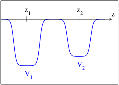
Figure 1: A schematic view of a two-center potential given by Eq. (1).

We consider a single-particle motion of a particle with mass $m$ in a potential which consists of two potential wells located at $z_{1}$ and $z_{2}$ on the $z$-axis (see Fig. 1):

$$V(\mbox{\boldmath$r$})=V_{1}(\mbox{\boldmath$r$}-z_{1}\mbox{\boldmath$e$}_{z})+V_{2}(\mbox{\boldmath$r$}-z_{2}\mbox{\boldmath$e$}_{z}),$$ (1)

where $\mbox{\boldmath$e$}_{z}$ is the unit vector in the $z$-direction. We first notice that the shifted potentials can be expressed as GGR77 ; MR86 ,

$$V_{s}(\mbox{\boldmath$r$}-z_{s}\mbox{\boldmath$e$}_{z})=e^{-i\hat{p}_{z}z_{s}/\hbar}\,V_{s}(\mbox{\boldmath$r$})\,e^{i\hat{p}_{z}z_{s}/\hbar}~{}~{}~{}~{}(s=1,2),$$ (2)

where $\hat{p}_{z}$ is the usual momentum operator for the $z$-direction. The idea of the separable expansion method GKR79 ; MR86 ; GGR77 is to expand the potentials $V_{s}$ on some basis as,

$$V_{s}(\mbox{\boldmath$r$}) = \sum_{\alpha,\alpha^{\prime}}\,|\Psi_{\alpha}\rangle\langle\Psi_{\alpha}|V_{s}|\Psi_{\alpha^{\prime}}\rangle\langle\Psi_{\alpha^{\prime}}|,$$ (3)

$$\equiv \sum_{\alpha,\alpha^{\prime}}\,|\Psi_{\alpha}\rangle\,V_{\alpha\alpha^{\prime}}^{(s)}\,\langle\Psi_{\alpha^{\prime}}|,$$ (4)

where $\{|\Psi_{\alpha}\rangle\}$ is a set of the basis functions (one could use different basis sets between $V_{1}$ and $V_{2}$, but here we use the same basis in order to simplify the notation). The single-particle potential, Eq. (1), then reads,

$$V=\sum_{s=1,2}\sum_{\alpha,\alpha^{\prime}}\,e^{-i\hat{p}_{z}z_{s}/\hbar}\,|\Psi_{\alpha}\rangle\,V_{\alpha\alpha^{\prime}}^{(s)}\,\langle\Psi_{\alpha^{\prime}}|\,e^{i\hat{p}_{z}z_{s}/\hbar}.$$ (5)

In Refs. GKR79 ; MR86 ; GGR77 , the Schrödinger equation with the potential given by Eq. (5), that is,

$$\left(\frac{\mbox{\boldmath$p$}^{2}}{2m}+V(\mbox{\boldmath$r$})-E\right)\Psi(\mbox{\boldmath$r$})=0,$$ (6)

where $\Psi$ is a single-particle wave function, is first transformed to the Lippmann-Schwinger equation. For a bound state, it reads,

$$|\Psi\rangle=\frac{1}{E-\frac{\mbox{\boldmath$p$}^{2}}{2m}}\,V|\Psi\rangle=G_{0}(E)\,V|\Psi\rangle,$$ (7)

where

$$G_{0}(E)=\frac{1}{E-\frac{\mbox{\boldmath$p$}^{2}}{2m}},$$ (8)

is the Green’s function. From this equation, one obtains,

$$\sum_{s^{\prime}}\sum_{\beta}\left[\delta_{s,s^{\prime}}\delta_{\alpha,\beta}\right.$$

$$\left.-\sum_{\alpha^{\prime}}\langle\Psi_{\alpha}|G_{0}(E)e^{i\hat{p}_{z}(z_{s}-z_{s^{\prime}})}|\Psi_{\alpha^{\prime}}\rangle V_{{\alpha^{\prime}}\beta}^{(s^{\prime})}\right]x_{\beta s^{\prime}}=0,$$ (9)

with $x_{\alpha s}\equiv\langle\Psi_{\alpha}|e^{i\hat{p}_{z}z_{s}/\hbar}|\Psi\rangle$. The eigen-values $E$ can be found by requiring that the determinant of the matrix in Eq. (9) vanishes at $E$ GKR79 ; MR86 ; GGR77 .

This method has been employed in several applications in the past. For instance, the author of Ref. Diaz-Torres08 used this method to discusses the two-center problem with arbitrarily oriented deformed potentials. It was also applied in Ref. MR86 to a problem of nucleon emission in heavy-ion collisions. However, as we have mentioned in the previous section, this method may have a difficulty when two eigen-energies are close to each other.

We therefore attempt to solve directly the Schrödinger equation, Eq. (6), with the separable representation of the single-particle potential, Eq. (5). To this end, we expand the single-particle wave function, $\Psi$, on a basis as,

$$|\Psi\rangle=\sum_{k}\,C_{k}|\tilde{\Psi}_{k}\rangle,$$ (10)

where the basis set $\{|\tilde{\Psi}_{k}\rangle\}$ is in general different from the basis set $\{|\Psi_{\alpha}\rangle\}$ for the potential. Using Eq. (5), one then obtains

$$\sum_{k,k^{\prime}}H_{kk^{\prime}}C_{k^{\prime}}=E\,C_{k},$$ (11)

with $H_{kk^{\prime}}=T_{kk^{\prime}}+V_{kk^{\prime}}$, where $T_{kk^{\prime}}$ and $V_{kk^{\prime}}$ are given by,

$$T_{kk^{\prime}}=\left\langle\tilde{\Psi}_{k}\left|\frac{\mbox{\boldmath$p$}^{2}}{2m}\right|\tilde{\Psi}_{k^{\prime}}\right\rangle,$$ (12)

and

$$V_{kk^{\prime}}=\sum_{s=1,2}\sum_{\alpha,\alpha^{\prime}}\,\langle\tilde{\Psi}_{k}|e^{-i\hat{p}_{z}z_{s}/\hbar}\,|\Psi_{\alpha}\rangle\,V_{\alpha\alpha^{\prime}}^{(s)}\,\langle\Psi_{\alpha^{\prime}}|\,e^{i\hat{p}_{z}z_{s}/\hbar}|\tilde{\Psi}_{k^{\prime}}\rangle,$$ (13)

respectively. The eigen-values and the eigen-functions are obtained by numerically diagonalizing the Hamiltonian matrix, $\{H_{kk^{\prime}}\}$. Notice that they can be obtained at once in this method, both for bound and continuum states, once the Hamiltonian matrix is constructed, whereas the matrix elements need to be constructed at each $E$ in the previous method. Note also that this method can easily be applied even in a situation when two eigen-values are close to each other. In general, one obtains both negative and positive energy states by the diagonalizing procedure. The positive wave functions so obtained well represent the inner part of scattering wave function at the same energy, even though the outer part reflects the properties of the basis functions and thus may not be well described. See e.g., Ref. HT70 .

II.2 Harmonic oscillator basis

In this paper, we consider a spherical central potential, together with a spin-orbit potential, for each of the potential wells, $V_{s}$. To be more specific, we consider a potential in a form of

$$V_{s}(r)=V^{(s)}_{0}(r)+V^{(s)}_{\rm ls}(r)\,\mbox{\boldmath$l$}\cdot\mbox{\boldmath$s$},$$ (14)

where $\mbox{\boldmath$l$}=\mbox{\boldmath$r$}\times\mbox{\boldmath$p$}/\hbar$ and $s$ are the orbital and the spin angular momenta, respectively, and $V^{(s)}_{0}(r)$ and $V^{(s)}_{\rm ls}(r)$ are assumed to depend only on $r=|\mbox{\boldmath$r$}|$. For this problem, we particularly employ a harmonic oscillator basis in the general formalism presented in the previous subsection. In the cylindrical coordinate, this basis is given by Vautherin73 ,

$$\Psi_{\alpha}(\mbox{\boldmath$r$})=\Psi_{n_{z}n_{\rho}\Lambda m_{s}}(\mbox{\boldmath$r$})=\phi_{n_{z}}(z)\,\psi_{n_{\rho}}^{(\Lambda)}(\rho)\,\frac{e^{i\Lambda\phi}}{\sqrt{2\pi}}\,\chi_{m_{s}},$$ (15)

where $\rho=\sqrt{x^{2}+y^{2}}$ with $x=\rho\cos\phi$ and $y=\rho\sin\phi$. Here, $\chi_{m_{s}}$ is the spin wave function, $m_{s}$ and $\Lambda$ being the $z$-component of the spin and the orbital angular momenta, respectively. The functions $\phi_{n_{z}}(z)$ and $\psi_{n_{\rho}}^{(\Lambda)}(\rho)$ in Eq. (15) are given by,

$$\phi_{n_{z}}(z) = \sqrt{\frac{1}{\sqrt{\pi}2^{n_{z}}n_{z}!}}\,b_{0}^{-1/2}\,e^{-\frac{z^{2}}{2b_{0}^{2}}}\,H_{n_{z}}(z/b_{0}),$$ (16)

$$\psi_{n_{\rho}}^{(\Lambda)}(\rho) = \sqrt{\frac{n_{\rho}!}{(n_{\rho}+\Lambda)!}}\,\frac{\sqrt{2}}{b_{0}}\,\left(\frac{\rho}{b_{0}}\right)^{\Lambda}\,e^{-\frac{\rho^{2}}{2b_{0}^{2}}}\,L_{n_{\rho}}^{(\Lambda)}(\rho^{2}/b_{0}^{2}),$$

respectively, where $H_{n_{z}}$ and $L_{n_{\rho}}^{(\Lambda)}$ are the Hermite polynomials and the associated Laguerre polynomials, respectively. $b_{0}=\sqrt{\hbar/(m\omega_{0})}$ is the oscillator length, with which the basis function satisfies the equation,

$$\left[\frac{\mbox{\boldmath$p$}^{2}}{2m}+\frac{1}{2}m\omega_{0}^{2}\,(\rho^{2}+z^{2})-\epsilon_{n_{z}n_{\rho}\Lambda}\right]\Psi_{n_{z}n_{\rho}\Lambda m_{s}}(\mbox{\boldmath$r$})=0,$$ (18)

with $\epsilon_{n_{z}n_{\rho}\Lambda}=(n_{z}+2n_{\rho}+\Lambda+3/2)\,\hbar\omega_{0}$. Notice that we employ the same oscillator length for the $z$ and $\rho$ directions, since the potentials, Eq. (14), are both spherical. The matrix elements of the potentials with this basis are given in Appendix.

For the basis for the wave functions, $\tilde{\Psi}_{k}$, we use the same harmonic oscillator basis as in Eq. (15) for the $\rho$-direction (with the same oscillator length, $b_{0}$) while we use a different function, $\tilde{\phi}_{\tilde{n}_{z}}(z)$, which is to be specific below, for the $z$-direction. That is, the basis for the wave functions reads,

$$\tilde{\Psi}_{k}(\mbox{\boldmath$r$})=\tilde{\Psi}_{\tilde{n}_{z}\tilde{n}_{\rho}\tilde{\Lambda}\tilde{m}_{s}}(\mbox{\boldmath$r$})=\tilde{\phi}_{\tilde{n}_{z}}(z)\,\psi_{\tilde{n}_{\rho}}^{(\tilde{\Lambda})}(\rho)\,\frac{e^{i\tilde{\Lambda}\phi}}{\sqrt{2\pi}}\,\chi_{\tilde{m}_{s}}.$$ (19)

The overlap integrals in the matrix elements for the single-particle potentials, Eq. (13), are then given by,

$$\langle\tilde{\Psi}_{k}|e^{-i\hat{p}_{z}z_{s}/\hbar}\,|\Psi_{\alpha}\rangle = \delta_{n_{\rho},\tilde{n}_{\rho}}\delta_{\Lambda,\tilde{\Lambda}}\delta_{m_{s},\tilde{m}_{s}}\,$$

$$\times\int^{\infty}_{-\infty}dz\,\tilde{\phi}_{\tilde{n}_{z}}(z)\phi_{n_{z}}(z-z_{s}),$$

where we have assumed that the basis function $\tilde{\phi}_{n}(z)$ is a real function of $z$. If one takes the harmonic oscillator basis, Eq. (16), for $\tilde{\phi}_{n}(z)$ (but with a different oscillator length from $b_{0}$), these overlap integrals can be computed analytically DW86 ; II98 ; Chang05 ; GME06 . Instead, we here use the eigen-functions for the one-dimensional central potential,

$$V_{z}(z)=V_{0}^{(1)}(|z-z_{1}|)+V_{0}^{(2)}(|z-z_{2}|),$$ (21)

which satisfy the one-dimensional Schrödinger equation of,

$$\left(-\frac{\hbar^{2}}{2m}\,\frac{d^{2}}{dz^{2}}+V_{z}(z)-\epsilon_{z}\right)\tilde{\phi}_{\tilde{n}_{z}}(z)=0.$$ (22)

Here, we use only the central part of the three-dimensional potential, Eq. (14). We solve this equation numerically with the Numerov method Koonin in order to obtain the basis functions, $\tilde{\phi}_{\tilde{n}_{z}}(z)$. The continuum states may be discretized by imposing the box boundary condition at $z=\pm z_{\rm box}$.

III Application to ¹⁶O+¹⁶O system

We now apply the new method for the two-center shell model to an actual problem. For this purpose, we consider neutron single-particle states in the ¹⁶O+¹⁶O system Diaz-Torres07 ; ZM76 ; GGR77 . The two potential wells, Eq. (14), are then identical to each other, that is, $V_{1}(r)=V_{2}(r)$. For these potential wells, we employ the Woods-Saxon form, that is,

$$V_{1}(r)=V_{2}(r) = V_{0}\left(1-\kappa(\mbox{\boldmath$l$}\cdot\mbox{\boldmath$s$})\frac{1}{r}\frac{d}{dr}\right)$$ (23)

$$~{}~{}~{}\times\left[1+\exp\left(\frac{r-R}{a}\right)\right]^{-1}.$$

We use the same values for the parameters as those in Ref. MR86 , that is, $V_{0}=-50.2$ MeV, $R=1.24\times 16^{1/3}$ fm, $\kappa=0.524$ fm², and $a=0.63$ fm, together with $m=939.6$ MeV/$c^{2}$.

We take into account the volume conservation condition in a similar way as in Refs. Diaz-Torres05 ; NSP87 . That is, the parameters $V_{0}$ and $R$ in the Woods-Saxon potential, Eq. (23), are adjusted at each separation distance, $z=|z_{1}-z_{2}|$, so that the two-center potential given by Eq. (1) is smoothly connected to a one-center potential for the ³²S nucleus as the separation distance is decreased to zero. For this purpose, we assume the same Woods-Saxon potential for ³²S as in Eq. (23) with the same value of $\kappa$ and $a$, while the radius parameter is modified to $R=1.24\times 32^{1/3}$ fm. For this potential, the depth parameter, $V_{0}$, is slightly adjusted to be $V_{0}=-51.823$ MeV so that the volume conservation condition is satisfied (see below). In order to determine the value of the parameters at intermediate distances, we interpolate the parameters $V_{0}$ and $1/R$ between those at $z=0$ and $z=\infty$ Diaz-Torres05 ; NSP87 , that is,

$$V_{0} = (1-x)\,V_{0}(^{32}{\rm S})+x\,V_{0}(^{16}{\rm O}),$$ (24)

$$\frac{1}{R} = (1-x)\,\frac{1}{R(^{32}{\rm S})}+x\,\frac{1}{R(^{16}{\rm O})},$$ (25)

where $V_{0}(^{32}{\rm S})$ and $R(^{32}{\rm S})$ are the depth and the radius parameters for the ³²S nucleus, respectively, while $V_{0}(^{16}{\rm O})$ and $R(^{16}{\rm O})$ are those for the ¹⁶O nucleus. The value of $x$ is determined by imposing the volume conservation condition given by,

$$\int d\mbox{\boldmath$r$}\,\theta\left[W_{0}-\tilde{V}_{0}(\mbox{\boldmath$r$};z_{1},z_{2})\right]\,\tilde{V}_{0}(\mbox{\boldmath$r$};z_{1},z_{2})={\rm const.},$$ (26)

with

$$\tilde{V}_{0}(\mbox{\boldmath$r$};z_{1},z_{2})\equiv V_{0}^{(1)}(|\mbox{\boldmath$r$}-z_{1}\mbox{\boldmath$e$}_{z}|)+V_{0}^{(2)}(|\mbox{\boldmath$r$}-z_{2}\mbox{\boldmath$e$}_{z}|),$$ (27)

where we take only the central part of the potential Diaz-Torres05 . In Eq. (26), $\theta$ is a step function and $W_{0}$ is a constant, for which we take $-12$ MeV so that the value of $W_{0}$ is around the Fermi energy for the ³²S nucleus. Notice that, in contrast to Refs. Diaz-Torres05 ; NSP87 , we take into account in Eq. (26) the effect of finite surface diffuseness by evaluating the volume integral of the potential. We find that this is important in order to keep the depth parameter in a Woods-Saxon potential similarly to each other between ¹⁶O and ³²S. Notice also that we interpolate the inverse of the radius parameter, $1/R$, rather than the radius parameter itself. We find that this scheme is more convenient for our purpose, as, at large distances $z$, the interpolation with $R$ with the volume conservation of Eq. (26) tends to lead to a wider and shallower potential than the potential given by Eq. (23), which however has the same volume integral to each other. This problem seems to disappear if the interpolation is carried out with the parameter $1/R$ rather than $R$.

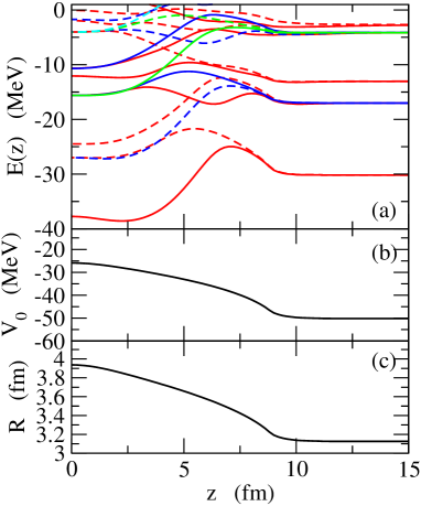
Figure 2: (a) Neutron single-particle energies for the ¹⁶O+¹⁶O system as a function of the separation distance between the two ¹⁶O nuclei. The solid and the dashed lines indicate the energies for the positive and the negative parity states, respectively. (b) The dependence of the depth parameter, $V_{0}$, in the Woods-Saxon potential on the separation distance as determined from the volume conservation condition given by Eq. (26). (c) The same as the panel (b), but for the radius parameter, $R$.

The top panel of Fig. 2 shows the neutron single-particle energies so obtained as a function of the separation distance $z$ between the two potential wells, which are placed at $z_{1}=-z/2$ and $z_{2}=z/2$, respectively. The $z$-dependence of the depth and the radius parameters in the Woods-Saxon potentials are also shown in the middle and the bottom panels, respectively. Since the two-center potential is axially symmetric around the $z$-axis, and also it is symmetric with respect to the parity transformation, the $z$-component of the total angular momentum, $j_{z}=\Lambda+m_{s}$, as well as the parity, $\pi$, are good quantum numbers to characterize the single-particle states. In the figure, the positive and negative parity states are indicated by the solid and the dashed lines, respectively. To obtain these energies, we expand each potential on the harmonic oscillator potential within 12 major shells, for which the frequency of the harmonic oscillator is taken to be $\hbar\omega_{0}=41\times 16^{-1/3}$ MeV. We have confirmed that the results do not change significantly even when a larger number of basis states are taken into account. For the expansion of the single-particle wave functions, we include the eigen-functions given by Eq. (22) up to $\epsilon_{z}=20$ MeV, where the continuum states are discretized with the box boundary condition, with the box size of $z_{\rm box}=z/2+10$ fm. As one can see, well-known features of single-particle energies in a symmetric two-center potential ZM76 ; MR86 ; GGR77 are well reproduced also in this calculation. That is, at large separation distances, positive and negative parity states are degenerate in energy, as they correspond to the symmetric and the anti-symmetric combinations of the wave function for the same state in the right and the left potential wells, respectively. As the separation distance decreases, these states are bifurcated, and the positive (negative) parity combination is converged to one of the positive-parity (negative-parity) single-particle states in the unified system in the limit of zero separation distance. At the intermediate separation distances, one can see a few avoided level crossings in a pair of single-particle states with the same parity and $j_{z}$.

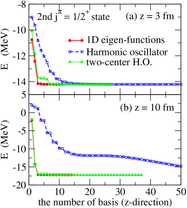
Figure 3: The single-particle energy for the second positive-parity state with $j_{z}^{\pi}=1/2^{+}$ as a function of the number of basis states in Eq. (19) for the $z$-direction. The upper and the lower panes show the result at the separation distance of $z=3$ fm and $z=10$ fm, respectively. The solid lines with filled circles indicate the results with the eigen-solutions for the one-dimensional two-center potentials given by Eq. (22), while the dashed lines and the solid lines with filled triangles show the results with one-center and two-center harmonic oscillator bases, respectively.

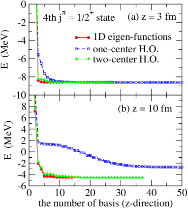
Figure 4: Same as Fig. 3, but for the 4th positive-parity state with $j_{z}^{\pi}=1/2^{+}$.

The convergence feature of the calculation is shown by the solid line with filled circles in Figs. 3 and 4. These are the single-particle energies for the second and the fourth positive-parity states with $j_{z}^{\pi}=1/2^{+}$ (see Fig. 2(a)), respectively, at $z=3$ fm (the upper panel) and at $z=10$ fm (the lower panel) as a function of the number of the basis states in Eq. (19) for the $z$-direction. For a comparison, we also show the results with a one-dimensional harmonic oscillator basis with a single center (the dashed line) and a double center (the solid line with filled triangles). The former is obtained with the oscillator length of $b_{z}={\rm max}(z,b_{0})$, where ${\rm max}(a,b)=a$ for $a\geq b$ and ${\rm max}(a,b)=b$ for $a<b$, while the latter uses the same oscillator length as the one used to expand the potential. Notice that the latter basis can be constructed analytically with confluent hypergeometric functions HMG69 . As expected, the convergence is fast for this calculation, while a similar good convergence is achieved also with a two-center harmonic oscillator basis. That is, the energy is almost converged by including only a few eigen-functions in the $z$-direction, both at $z=3$ fm and $z=10$ fm. In contrast, the convergence is considerably slow with the single-center harmonic oscillator basis, especially at large separation distances. Evidently, the method proposed in this paper provides a powerful way to solve the two-center shell model with arbitrary finite depth potential wells.

IV Summary

We have proposed a novel method to solve the eigen-value problem for a single-particle motion in a two-center potential. This method combines the separable representation for the single-particle potential with the usual matrix diagonalization. To this end, we have expanded the potential on a harmonic oscillator basis while the single-particle wave functions on the combined basis of a harmonic oscillator and eigen-functions of a one-dimensional two-center potential. In this way, the method can be applied easily and efficiently even to a situation with two close single-particle energies. Also, with this method both bound and resonance states can be obtained in a single framework.

In this paper, we have considered a two-center potential which consists of two shifted spherical Woods-Saxon potentials. It would be an interesting future problem to extend the present approach to a two-center potential with deformed potentials NSP87 ; Diaz-Torres08 . Such extension would be useful in order to understand the reaction dynamics for hot fusion reactions to synthesize superheavy elements, in which ⁴⁸Ca beams are used together with a deformed actinide target nucleus OU15 ; HHO13 .

Appendix A Matrix elements of Hamiltonian with the harmonic oscillator basis

In this Appendix, we present matrix elements of the Hamiltonian with a spherical potential, Eq. (14), with the harmonic oscillator basis, Eq. (15), in the cylindrical coordinate. To this end, we closely follow Sec. IV-C in Ref. Vautherin73 .

A.1 Central potential

We first consider the central part of the potential, $V_{0}^{(s)}(r)$. Its matrix elements read,

$$\langle\Psi_{\alpha}|V_{0}^{(s)}|\Psi_{\alpha^{\prime}}\rangle = \delta_{\Lambda,\Lambda^{\prime}}\delta_{m_{s},m_{s}^{\prime}}$$ (28)

$$\times\int^{\infty}_{-\infty}dz\int^{\infty}_{0}\rho d\rho\,V_{0}^{(s)}(r)\,\phi_{n_{z}}(z)\phi_{n_{z}^{\prime}}(z)$$

$$\times\psi_{n_{\rho}}^{(\Lambda)}(\rho)\psi_{n_{\rho}^{\prime}}^{(\Lambda^{\prime})}(\rho),$$

with $r=\sqrt{\rho^{2}+z^{2}}$.

A.2 Spin-orbit potential

We next consider the spin-orbit potential, $V_{\rm ls}^{(s)}(r)\,\mbox{\boldmath$l$}\cdot\mbox{\boldmath$s$}$. We first note that the basis function $|\Psi_{\alpha}\rangle$ is an eigen-function of $l_{z}$ and $s_{z}$ as,

$$l_{z}\Psi_{\alpha} = \frac{1}{i}\,\frac{\partial}{\partial\phi}\,\Psi_{\alpha}=\Lambda\Psi_{\alpha},$$ (29)

$$s_{z}\Psi_{\alpha} = m_{s}\,\Psi_{\alpha}.$$ (30)

We also notice that

$$\mbox{\boldmath$l$}\cdot\mbox{\boldmath$s$}=\frac{1}{2}(l_{+}s_{-}+l_{-}s_{+})+l_{z}s_{z},$$ (31)

with $s_{\pm}=s_{x}\pm is_{y}$ and

$$l_{\pm} = l_{x}\pm il_{y},$$ (32)

$$= \mp e^{\pm i\phi}\left(\rho\frac{\partial}{\partial z}-z\frac{\partial}{\partial\rho}\pm\frac{z}{\rho}\,\frac{1}{i}\frac{\partial}{\partial\phi}\right).$$ (33)

Since $s_{+}\chi_{\downarrow}=\chi_{\uparrow}$, $s_{-}\chi_{\uparrow}=\chi_{\downarrow}$, and

$$\int^{2\pi}_{0}\frac{e^{-i\Lambda\phi}}{\sqrt{2\pi}}\,(\mp e^{\pm i\phi})\,\frac{e^{i\Lambda^{\prime}\phi}}{\sqrt{2\pi}}=\mp\delta_{\Lambda,\Lambda^{\prime}\pm 1},$$ (34)

one obtains,

$$\langle\Psi_{n_{z}n_{\rho}\Lambda m_{s}}|V_{\rm ls}^{(s)}(r)\mbox{\boldmath$l$}\cdot\mbox{\boldmath$s$}|\Psi_{n^{\prime}_{z}n^{\prime}_{\rho}\Lambda^{\prime}m_{s}}\rangle$$

$$\quad=\delta_{\Lambda,\Lambda^{\prime}}$$

$$\quad\times\Lambda m_{s}\,\int^{\infty}_{-\infty}dz\int^{\infty}_{0}\rho d\rho\,V_{\rm ls}^{(s)}(r)\,\phi_{n_{z}}(z)\phi_{n_{z}^{\prime}}(z)$$

$$\quad\times\psi_{n_{\rho}}^{(\Lambda)}(\rho)\psi_{n_{\rho}^{\prime}}^{(\Lambda^{\prime})}(\rho),$$ (35)

$$\langle\Psi_{n_{z}n_{\rho}\Lambda\downarrow}|V_{\rm ls}^{(s)}(r)\mbox{\boldmath$l$}\cdot\mbox{\boldmath$s$}|\Psi_{n^{\prime}_{z}n^{\prime}_{\rho}\Lambda^{\prime}\uparrow}\rangle$$

$$\quad=-\frac{1}{2}\,\delta_{\Lambda,\Lambda^{\prime}+1}$$

$$\quad\times\int^{\infty}_{-\infty}dz\int^{\infty}_{0}\rho d\rho\,V_{\rm ls}^{(s)}(r)\,\phi_{n_{z}}(z)\psi_{n_{\rho}}^{(\Lambda)}(\rho)$$

$$\quad\times\left(\rho\frac{\partial}{\partial z}-z\frac{\partial}{\partial\rho}+\frac{z}{\rho}\,\Lambda^{\prime}\right)\phi_{n_{z}^{\prime}}(z)\psi_{n_{\rho}^{\prime}}^{(\Lambda^{\prime})}(\rho),$$ (36)

and

$$\langle\Psi_{n_{z}n_{\rho}\Lambda\uparrow}|V_{\rm ls}^{(s)}(r)\mbox{\boldmath$l$}\cdot\mbox{\boldmath$s$}|\Psi_{n^{\prime}_{z}n^{\prime}_{\rho}\Lambda^{\prime}\downarrow}\rangle$$

$$\quad=\frac{1}{2}\,\delta_{\Lambda,\Lambda^{\prime}-1}$$

$$\quad\times\int^{\infty}_{-\infty}dz\int^{\infty}_{0}\rho d\rho\,V_{\rm ls}^{(s)}(r)\,\phi_{n_{z}}(z)\psi_{n_{\rho}}^{(\Lambda)}(\rho)$$

$$\quad\times\left(\rho\frac{\partial}{\partial z}-z\frac{\partial}{\partial\rho}-\frac{z}{\rho}\,\Lambda^{\prime}\right)\phi_{n_{z}^{\prime}}(z)\psi_{n_{\rho}^{\prime}}^{(\Lambda^{\prime})}(\rho).$$ (37)

A.3 Kinetic energy

The matrix elements for the kinetic energy for the $z$-direction is computed as

$$\left\langle\Psi_{\alpha}\left|\frac{p_{z}^{2}}{2m}\right|\Psi_{\alpha^{\prime}}\right\rangle = -\frac{\hbar^{2}}{2m}\,\delta_{n_{\rho},n^{\prime}_{\rho}}\delta_{\Lambda,\Lambda^{\prime}}\delta_{m_{s},m_{s}^{\prime}}$$

$$\times\int^{\infty}_{-\infty}dz\,\phi_{n_{z}}(z)\frac{d^{2}\phi_{n_{z}^{\prime}}(z)}{dz^{2}}.$$

$$= \frac{\hbar^{2}}{2m}\,\delta_{n_{\rho},n^{\prime}_{\rho}}\delta_{\Lambda,\Lambda^{\prime}}\delta_{m_{s},m_{s}^{\prime}}$$

$$\times\int^{\infty}_{-\infty}dz\,\frac{d\phi_{n_{z}}(z)}{dz}\frac{d\phi_{n_{z}^{\prime}}(z)}{dz}.$$

Here, we keep the matrix elements in a general form, so that the formula can be applied also to Eq. (12) with Eq. (19).

In order to evaluate the matrix elements for the kinetic energy for the $\rho$-direction, we use the Schrödinger equation of,

$$\left(\frac{p_{x}^{2}+p_{y}^{2}}{2m}+\frac{1}{2}m\omega_{0}^{2}\rho^{2}-\epsilon_{n_{\rho}\Lambda}\right)\Psi_{\alpha}(\mbox{\boldmath$r$})=0,$$ (39)

with $\epsilon_{n_{\rho}\Lambda}=(2n_{\rho}+\Lambda+1)\,\hbar\omega_{0}$. This leads to,

$$\left\langle\Psi_{\alpha}\left|\frac{p_{x}^{2}+p_{y}^{2}}{2m}\right|\Psi_{\alpha^{\prime}}\right\rangle$$

$$=\epsilon_{n_{\rho}\Lambda}\,\delta_{\alpha,\alpha^{\prime}}$$

$$-\delta_{n_{z},n^{\prime}_{z}}\delta_{\Lambda,\Lambda^{\prime}}\delta_{m_{s},m_{s}^{\prime}}\,$$

$$\quad\times\int^{\infty}_{0}\rho d\rho\,\left(\frac{1}{2}m\omega_{0}^{2}\rho^{2}\right)\psi_{n_{\rho}}^{(\Lambda)}(\rho)\psi_{n_{\rho}^{\prime}}^{(\Lambda^{\prime})}(\rho).$$ (40)

References

- (1) W. Greiner, J.Y. Park, and W. Scheid, Nuclear Molecules (World Scientific, Singapore, 1994).
- (2) J. Maruhn and W. Greiner, Z. Phys. 251, 431 (1972).
- (3) R.A. Gherghescu, Phys. Rev. C67, 014309 (2003).
- (4) D. Glas and U. Mosel, Phys. Lett. 49B, 301 (1974); Nucl. Phys. A264, 268 (1976).
- (5) G. Schütte and L. Wilets, Nucl. Phys. A252, 21 (1975).
- (6) T. Ichikawa and K. Matsuyanagi, Phys. Rev. C88, 011602(R) (2013); Phys. Rev. C92, 021602(R) (2015).
- (7) A. Diaz-Torres, Phys. Rev. C69, 021603(R) (2004).
- (8) A. Diaz-Torres, L.R. Gasques, and M. Wiescher, Phys. Lett. B652, 255 (2007).
- (9) F.A. Ivanyuk, S. Chiba, and Y. Aritomo, Phys. Rev. C90, 054607 (2014).
- (10) V.I. Zagrebaev and W. Greiner, Nucl. Phys. A944, 257 (2015).
- (11) P. Holzer, U. Mosel, and W. Greiner, Nucl. Phys. A138, 241 (1969).
- (12) P.G. Zint and U. Mosel, Phys. Rev. C14, 1488 (1976).
- (13) K. Pruess and P. Lichtner, Nucl. Phys. A291, 475 (1977).
- (14) R.W. Hasse, Nucl. Phys. A229, 141 (1974).
- (15) P. Bergmann and H.-J. Scheefer, Z. Natur. A29, 1003 (1974).
- (16) P.-T. Ong and W. Scheid, Z. Natur. A30, 406 (1975).
- (17) G. Nuhn, W. Scheid, and J.Y. Park, Phys. Rev. C35, 2146 (1987).
- (18) F.A. Gareev, M. Ch. Gizzatkulov, and J. Revai, Nucl. Phys. A286, 512 (1977).
- (19) B. Milek and R. Reif, Nucl. Phys. A458, 354 (1986).
- (20) B. Gyarmati, A.T. Kruppa, and J. Revai, Nucl. Phys. A326, 119 (1979).
- (21) A. Diaz-Torres and W. Scheid, Nucl. Phys. A757, 373 (2005).
- (22) A. Diaz-Torres, Phys. Rev. Lett. 101, 122501 (2008).
- (23) V. Tornow, P.-G. Reinhard, and D. Drechsel, Z. Phys. A280, 253 (1977).
- (24) A. Diaz-Torres, Phys. Lett. B594, 69 (2004).
- (25) A.U. Hazi and H.S. Taylor, Phys. Rev. A1, 1109 (1970).
- (26) D. Vautherin, Phys. Rev. C7, 296 (1973).
- (27) P.J. Drallos and J.M. Wadehra, J. Chem. Phys. 85, 6524 (1986).
- (28) F. Iachello and M. Ibrahim, J. Phys. Chem. A102, 9427 (1998).
- (29) J.-L. Chang, J. of Mol. Spec. 232, 102 (2005).
- (30) I.I. Guseinov, B.A. Mamedov, and A.S. Ekenoglu, Z. Natur. A61, 141 (2006); Comp. Phys. Comm. 175, 226 (2006).
- (31) S.E. Koonin and D.C. Meredith, Computational Physics (Addison-Weseley, Reading, MA, 1990).
- (32) Yu. Ts. Oganessian and V.K. Utyonkov, Nucl. Phys. A944, 62 (2015).
- (33) J.H. Hamilton, S. Hofmann, and Y.T. Oganessian, Annu. Rev. Nucl. Part. Sci. 63, 383 (2013).