Parallel Simultaneous Perturbation Optimization

Atiye Alaeddini  and  Daniel J. Klein
Abstract.

Stochastic computer simulations enable users to gain new insights into complex physical systems. Optimization is a common problem in this context: users seek to find model inputs that maximize the expected value of an objective function. The objective function, however, is time-intensive to evaluate, and cannot be directly measured. Instead, the stochastic nature of the model means that individual realizations are corrupted by noise. More formally, we consider the problem of optimizing the expected value of an expensive black-box function with continuously-differentiable mean, from which observations are corrupted by Gaussian noise. We present Parallel Simultaneous Perturbation Optimization (PSPO), which extends a well-known stochastic optimization algorithm, simultaneous perturbation stochastic approximation, in several important ways. Our modifications allow the algorithm to fully take advantage of parallel computing resources, like high-performance cloud computing. The resulting PSPO algorithm takes fewer time-consuming iterations to converge, automatically chooses the step size, and can vary the error tolerance by step. Theoretical results are supported by a numerical example. To demonstrate the performance of the algorithm, we implemented the algorithm to maximize the pseudo-likelihood of a stochastic epidemiological model to data of a measles outbreak.

1. Introduction

Stochastic optimization is of core practical importance in many fields of science and engineering. For instance, epidemiological systems involve individuals subject to exogenous disturbances, which emphasizes the need for models and methods capable of dealing with stochasticity. While many optimization methodologies exist for deterministic systems, these algorithms can give misleading results when applied to stochastic systems. Closed-form solutions do not generally exist for stochastic optimization problems, thus we seek an iterative algorithm which guarantees convergence to the local optimal point.

Many approximation algorithms have been developed to solve a wide variety of deterministic or stochastic problems. The steepest descent method (Wright and Nocedal, 1999) is the most prominent iterative method for optimizing a complex objective function. The gradient-based algorithms, such as Robbins-Monro (Robbins and Monro, 1951), Newton-Raphson (Fröberg, 1969), and neural network back-propagation (Rumelhart et al., 1985), rely on direct measurements of the gradient of the objective function with respect to the optimization parameter. But, in many cases the gradient of the loss function is not available. This is a common occurrence, for example, in complex systems, such as the optimization problems given in (Tsilifis et al., 2017; Alaeddini and Klein, 2017), the exact functional relationship between the loss function value and the parameters is not known, and the loss function is evaluated by measurements on the system or by running simulation. A review on the main areas of optimization via simulation can be found in (Fu, 1994; Hong and Nelson, 2009; Swisher et al., 2000).

Some algorithms have been developed specifically to optimize stochastic black-box cost functions. Of these, the Kiefer-Wolfowitz algorithm (Kiefer et al., 1952) is perhaps the most well known. This algorithm estimates the gradient from noisy measurements using finite differencing. Another well known stochastic optimization algorithm in the case of high dimensional problems is Simultaneous Perturbation Stochastic Approximation (SPSA), which is an approximation algorithm based on simultaneous perturbation (Spall, 1992). Later, J. C. Spall presented a second-order variant of SPSA (Spall, 2000). The SPSA algorithm is used extensively in many different areas, e.g.  signal timing for traffic control (Ma et al., 2013), and some large scale machine learning problems (Byrd et al., 2011). The convergence of this algorithm to the optimal value in the stochastic almost sure sense makes it suitable in many applications.

The stochastic nature of some complex models, e.g.  epidemiological models, means that each set of parameters maps to a distribution of outcomes, from which each sample (model run) can take several hours to obtain. In the quick-to-evaluate deterministic model setting, almost any classical optimization algorithm, such as steepest descent or Newton-Raphson, can be used. However, care must be taken when applying deterministic methods to stochastic objective functions, as the inherent noise causes unexpected behavior. In this paper, we introduce PSPO, an algorithm for optimization of stochastic objective functions. Despite many advantageous properties of the SPSA algorithm, mentioned earlier, it is a serial algorithm that evaluates the (stochastic) function a few points at a time, which results in low convergence rate. Researchers have looked at ways of enhancing the convergence of the SPSA algorithm, e.g.  iterate averaging is an approach aimed at achieving higher convergence rate in a stochastic setting (Polyak and Juditsky, 1992), using deterministic parameter perturbations instead of random perturbations (Bhatnagar et al., 2003), and more (Kocsis and Szepesvári, 2006; Spall, 2009).

The PSPO algorithm, introduced in this paper, takes advantage of fundamentally-parallel resources like high-performance cloud-based computing. Our method is appropriate for problems with very noisy gradients. We also derive a relationship between the number of parallel rounds of computation and error tolerance of the gradient for each iteration. The main contribution of this paper is introducing a stochastic optimization algorithm which can be easily implemented on parallel computers, and to provide the minimum number of parallel computers in order to have an upper-bound on the error for each iteration. We demonstrate that PSPO works well in practice and compares favorably to the conventional simultaneous perturbation optimization algorithm (SPSA). The rest of the paper is structured as follows. In Section 2, we give a review of the simultaneous perturbation optimization algorithm. The Parallel Simultaneous Perturbation Optimization (PSPO) algorithm is presented in Section 3. The numerical simulations are given in Section 4, and Section 5 concludes the paper.

2. Preliminaries

Consider the problem of minimizing a cost function L(θ):p:𝐿𝜃superscript𝑝L(\theta):\mathbb{R}^{p}\rightarrow\mathbb{R}. Spall (Spall, 1992, 2000, 2009) presented an efficient stochastic algorithm called Simultaneous Perturbation Stochastic Approximation (SPSA). The SPSA algorithm estimates the gradient and the Hessian matrix by finite difference. This algorithm basically consists of two parallel recursions for estimating the optimization parameter, θ𝜃\theta, and the Hessian matrix, H(θ)𝐻𝜃H(\theta). The first recursion is a stochastic equivalence of the Newton-Raphson algorithm, and the second one estimates the Hessian matrix. These two recursions are

(1) θk+1=θkak(Π𝒫(H¯k))1𝐠^k(θk),subscript𝜃𝑘1subscript𝜃𝑘subscript𝑎𝑘superscriptsubscriptΠ𝒫subscript¯𝐻𝑘1subscript^𝐠𝑘subscript𝜃𝑘\displaystyle\theta_{k+1}=\theta_{k}-a_{k}\left(\Pi_{\mathcal{P}}(\bar{H}_{k})\right)^{-1}\hat{\mathbf{g}}_{k}(\theta_{k})\,,
H¯k=kk+1H¯k1+1k+1H^k,subscript¯𝐻𝑘𝑘𝑘1subscript¯𝐻𝑘11𝑘1subscript^𝐻𝑘\displaystyle\bar{H}_{k}=\frac{k}{k+1}\bar{H}_{k-1}+\frac{1}{k+1}\hat{H}_{k}\,,

where aksubscript𝑎𝑘a_{k} is a positive scalar factor, 𝒫𝒫\mathcal{P} denotes the set of all positive definite matrices, and Π𝒫()subscriptΠ𝒫\Pi_{\mathcal{P}}(\cdot) is the projection into the admissible set 𝒫𝒫\mathcal{P}. Here, 𝐠^ksubscript^𝐠𝑘\hat{\mathbf{g}}_{k} and H^ksubscript^𝐻𝑘\hat{H}_{k} are the estimated gradient and Hessian at iteration k𝑘k. The SPSA approach for estimating the 𝐠^k(θ)subscript^𝐠𝑘𝜃\hat{\mathbf{g}}_{k}(\theta) and H^k(θ)subscript^𝐻𝑘𝜃\hat{H}_{k}(\theta) follows.

Let ΔkpsubscriptΔ𝑘superscript𝑝\Delta_{k}\in\mathbb{R}^{p} be vectors of p𝑝p mutually independent zero-mean random variables satisfying the condition of E{Δk1}𝐸superscriptsubscriptΔ𝑘1E\{\Delta_{k}^{-1}\} be bounded. An admissible distribution is a Bernoulli ±1plus-or-minus1\pm 1 distribution. The positive scalars cksubscript𝑐𝑘c_{k} are chosen such that they usually get smaller as k𝑘k gets larger. The two-sided estimate of the gradient at iteration k𝑘k is given by:

(2) 𝐠^k(θk)=yk(+)yk()2ckΔk1,subscript^𝐠𝑘subscript𝜃𝑘superscriptsubscript𝑦𝑘superscriptsubscript𝑦𝑘2subscript𝑐𝑘superscriptsubscriptΔ𝑘1\hat{\mathbf{g}}_{k}(\theta_{k})=\frac{y_{k}^{(+)}-y_{k}^{(-)}}{2c_{k}}\Delta_{k}^{-1}\,,

where yk(±)superscriptsubscript𝑦𝑘plus-or-minusy_{k}^{(\pm)} are the noisy measurements of the cost function at θk±ckΔkplus-or-minussubscript𝜃𝑘subscript𝑐𝑘subscriptΔ𝑘\theta_{k}\pm c_{k}\Delta_{k}. Note that in (2), Δk1superscriptsubscriptΔ𝑘1\Delta_{k}^{-1} is the element-wise inverse of ΔksubscriptΔ𝑘\Delta_{k}. In the case of second order SPSA, it is suggested to use a one-sided gradient approximation, given by:

(3) 𝐠^k(θk)=yk(+)ykckΔk1.subscript^𝐠𝑘subscript𝜃𝑘superscriptsubscript𝑦𝑘subscript𝑦𝑘subscript𝑐𝑘superscriptsubscriptΔ𝑘1\hat{\mathbf{g}}_{k}(\theta_{k})=\frac{y_{k}^{(+)}-y_{k}}{c_{k}}\Delta_{k}^{-1}\,.

Now let Δ~kpsubscript~Δ𝑘superscript𝑝\tilde{\Delta}_{k}\in\mathbb{R}^{p} be vectors of p𝑝p mutually independent zero-mean random variables satisfying the same condition of ΔksubscriptΔ𝑘\Delta_{k}. The positive scalars c~ksubscript~𝑐𝑘\tilde{c}_{k} are also chosen such that they get smaller as k𝑘k gets larger. The numerical value of c~ksubscript~𝑐𝑘\tilde{c}_{k} is suggested to be chosen smaller than cksubscript𝑐𝑘c_{k}. The following formula gives a per-iteration estimate of the Hessian matrix.

(4) H^k=12[δGk2c~kΔ~k1+(δGk2c~kΔ~k1)T],subscript^𝐻𝑘12delimited-[]𝛿subscript𝐺𝑘2subscript~𝑐𝑘superscriptsubscript~Δ𝑘1superscript𝛿subscript𝐺𝑘2subscript~𝑐𝑘superscriptsubscript~Δ𝑘1𝑇\hat{H}_{k}=\frac{1}{2}\left[\frac{\delta G_{k}}{2\tilde{c}_{k}}\tilde{\Delta}_{k}^{-1}+\left(\frac{\delta G_{k}}{2\tilde{c}_{k}}\tilde{\Delta}_{k}^{-1}\right)^{T}\right]\,,

where

(5) δGk=𝐠^k(θk+c~kΔ~k)𝐠^k(θkc~kΔ~k).𝛿subscript𝐺𝑘subscript^𝐠𝑘subscript𝜃𝑘subscript~𝑐𝑘subscript~Δ𝑘subscript^𝐠𝑘subscript𝜃𝑘subscript~𝑐𝑘subscript~Δ𝑘\delta G_{k}=\hat{\mathbf{g}}_{k}(\theta_{k}+\tilde{c}_{k}\tilde{\Delta}_{k})-\hat{\mathbf{g}}_{k}(\theta_{k}-\tilde{c}_{k}\tilde{\Delta}_{k})\,.

The practical implementation details of the algorithm is presented in (Spall, 2000).

3. Parallel Simultaneous Perturbation Optimization: PSPO

While SPSA is an efficient optimization algorithm for high dimensional problems, it requires many iterations to converge, particularly for high-noise problems. In the case of high uncertain problems, the computation of the gradient and Hessian from noisy objective function evaluations benefits from more evaluations. The idea here is using parallel computing of the gradient and Hessian with different perturbation vectors, and use the estimated gradient and Hessian in a conjugate gradient type optimization algorithm.

3.1. Gradient Estimation

The gradient vector at each iteration can be obtained by performing multiple evaluations of (3) for different values of perturbation. Let 𝐠𝐠\mathbf{g} be the gradient at a point θ𝜃\theta, and 𝐠isuperscript𝐠𝑖\mathbf{g}^{i} represents the directional gradient in ΔisubscriptΔ𝑖\Delta_{i} direction at this point. Then we know that:

𝐠i=𝐠(θ),ΔiΔi2Δi.superscript𝐠𝑖𝐠𝜃subscriptΔ𝑖superscriptnormsubscriptΔ𝑖2subscriptΔ𝑖\mathbf{g}^{i}=\frac{\left<\mathbf{g}(\theta),\Delta_{i}\right>}{\|\Delta_{i}\|^{2}}\Delta_{i}\,.

Let 𝐠^isuperscript^𝐠𝑖\hat{\mathbf{g}}^{i} be the estimated gradient using the one-sided gradient approximation (3) and perturbation vector ΔisubscriptΔ𝑖\Delta_{i}. If ΔisubscriptΔ𝑖\Delta_{i} is a Bernoulli ±1plus-or-minus1\pm 1 vector, we have

𝐠^ip𝐠i=𝐠(θ),ΔiΔi𝐠^(θ),ΔiΔi.superscript^𝐠𝑖𝑝superscript𝐠𝑖𝐠𝜃subscriptΔ𝑖subscriptΔ𝑖^𝐠𝜃subscriptΔ𝑖subscriptΔ𝑖\hat{\mathbf{g}}^{i}\approx p\mathbf{g}^{i}=\left<\mathbf{g}(\theta),\Delta_{i}\right>\Delta_{i}\approx\left<\hat{\mathbf{g}}(\theta),\Delta_{i}\right>\Delta_{i}\,.

Then,

𝐠^TΔiδfic,superscript^𝐠𝑇subscriptΔ𝑖𝛿subscript𝑓𝑖𝑐\hat{\mathbf{g}}^{T}\Delta_{i}\approx\frac{\delta f_{i}}{c}\,,
δfi=L(θ+cΔi)L(θ),𝛿subscript𝑓𝑖𝐿𝜃𝑐subscriptΔ𝑖𝐿𝜃\delta f_{i}=L(\theta+c\Delta_{i})-L(\theta)\,,

and then,

(6) 𝐠^TΔ1c[δf1δf2δfM],superscript^𝐠𝑇Δ1𝑐matrix𝛿subscript𝑓1𝛿subscript𝑓2𝛿subscript𝑓𝑀\hat{\mathbf{g}}^{T}\Delta\approx\frac{1}{c}\begin{bmatrix}\delta f_{1}&\delta f_{2}&\cdots&\delta f_{M}\end{bmatrix}\,,

where,

Δ=[Δ1Δ2ΔM].ΔmatrixsubscriptΔ1subscriptΔ2subscriptΔ𝑀\Delta=\begin{bmatrix}\Delta_{1}&\Delta_{2}&\cdots&\Delta_{M}\end{bmatrix}\,.

If {Δi}1iMsubscriptsubscriptΔ𝑖1𝑖𝑀\{\Delta_{i}\}_{1\leq i\leq M} span psuperscript𝑝\mathbb{R}^{p}, then ΔΔTΔsuperscriptΔ𝑇\Delta\Delta^{T} is invertible. So, the least square estimation of 𝐠^^𝐠\hat{\mathbf{g}} is given by:

(7) 𝐠^1c(ΔΔT)1Δ[δf1δf2δfM]T.^𝐠1𝑐superscriptΔsuperscriptΔ𝑇1Δsuperscriptmatrix𝛿subscript𝑓1𝛿subscript𝑓2𝛿subscript𝑓𝑀𝑇\hat{\mathbf{g}}\approx\frac{1}{c}\left(\Delta\Delta^{T}\right)^{-1}\Delta\begin{bmatrix}\delta f_{1}&\delta f_{2}&\ldots&\delta f_{M}\end{bmatrix}^{T}\,.

On the other hand, if M<p𝑀𝑝M<p, then (6) is an under-determined system which has non-unique solutions. Then, the solution of the minimum Euclidean norm, 𝐠^2subscriptnorm^𝐠2\displaystyle\|\hat{\mathbf{g}}\|_{2}, among all solutions is given by:

(8) 𝐠^1cΔ(ΔTΔ)1[δf1δf2δfM]T.^𝐠1𝑐ΔsuperscriptsuperscriptΔ𝑇Δ1superscriptmatrix𝛿subscript𝑓1𝛿subscript𝑓2𝛿subscript𝑓𝑀𝑇\hat{\mathbf{g}}\approx\frac{1}{c}\Delta\left(\Delta^{T}\Delta\right)^{-1}\begin{bmatrix}\delta f_{1}&\delta f_{2}&\ldots&\delta f_{M}\end{bmatrix}^{T}\,.

The Parallel Simultaneous Perturbation (PSP) algorithm for estimating the gradient at a given point is given in Algorithm 1. In order to improve the efficiency of this algorithm, we can compute L(θ)𝐿𝜃L(\mathbf{\theta}) once, out of the loop. Doing this, we need M+1𝑀1M+1 function evaluations for estimating the gradient.

  Inputs: given point θ𝜃\theta, perturbation size c𝑐c, and # of parallel rounds M𝑀M
  Randomly sample Δ0subscriptΔ0\Delta_{0} from {±1}plus-or-minus1\{\pm 1\} binary distribution
  Initialize computation round counter i:=1assign𝑖1i:=1 and spare counter j:=1assign𝑗1j:=1
  while iM𝑖𝑀i\leq M do
     Δi:=(I2𝐞j𝐞jT)Δ0assignsubscriptΔ𝑖𝐼2subscript𝐞𝑗superscriptsubscript𝐞𝑗𝑇subscriptΔ0\Delta_{i}:=(I-2\mathbf{e}_{j}\mathbf{e}_{j}^{T})\Delta_{0}
     δfi(θ):=f(θ+cΔi)f(θ)assign𝛿subscript𝑓𝑖𝜃𝑓𝜃𝑐subscriptΔ𝑖𝑓𝜃\delta f_{i}(\theta):=f(\theta+c\Delta_{i})-f(\theta)
     if (imodp)=0modulo𝑖𝑝0(i\mod p)=0 then
        Reset j:=0assign𝑗0j:=0 and re-sample Δ0subscriptΔ0\Delta_{0} from {±1}plus-or-minus1\{\pm 1\} binary distribution
     end if
     i:=i+1assign𝑖𝑖1i:=i+1; j:=j+1assign𝑗𝑗1j:=j+1
  end while
  Δ:=[Δ1Δ2ΔM]assignΔmatrixsubscriptΔ1subscriptΔ2subscriptΔ𝑀\Delta:=\begin{bmatrix}\Delta_{1}&\Delta_{2}&\ldots&\Delta_{M}\end{bmatrix}
  if Mp𝑀𝑝M\geq p then
     𝐠^(θ):=1c(ΔΔT)1Δ[δf1δf2δfM]Tassign^𝐠𝜃1𝑐superscriptΔsuperscriptΔ𝑇1Δsuperscriptmatrix𝛿subscript𝑓1𝛿subscript𝑓2𝛿subscript𝑓𝑀𝑇\hat{\mathbf{g}}(\theta):=\frac{1}{c}\left(\Delta\Delta^{T}\right)^{-1}\Delta\begin{bmatrix}\delta f_{1}&\delta f_{2}&\ldots&\delta f_{M}\end{bmatrix}^{T}
  else
     𝐠^(θ):=1cΔ(ΔTΔ)1[δf1δf2δfM]Tassign^𝐠𝜃1𝑐ΔsuperscriptsuperscriptΔ𝑇Δ1superscriptmatrix𝛿subscript𝑓1𝛿subscript𝑓2𝛿subscript𝑓𝑀𝑇\hat{\mathbf{g}}(\theta):=\frac{1}{c}\Delta\left(\Delta^{T}\Delta\right)^{-1}\begin{bmatrix}\delta f_{1}&\delta f_{2}&\ldots&\delta f_{M}\end{bmatrix}^{T}
  end if
  return  𝐠^(θ)^𝐠𝜃\hat{\mathbf{g}}(\theta)
ALGORITHM 1 Parallel Simultaneous Perturbation (PSP) gradient estimation.

In Algorithm 1, we suggest an efficient strategy to choose independent ΔΔ\Delta vectors. First, we sample Δ0subscriptΔ0\Delta_{0} from a Bernoulli ±1plus-or-minus1\pm 1 distribution. In round j𝑗j, 1jp1𝑗𝑝1\leq j\leq p, we need to switch the sign of the j𝑗jth element in Δ0subscriptΔ0\Delta_{0} to generate ΔjsubscriptΔ𝑗\Delta_{j}. The same procedure repeats for the next p𝑝p rounds of computations.

Lemma 3.1.

Given the suggested procedure in Algorithm 1 for choosing ΔisubscriptΔ𝑖\Delta_{i} vectors, the vectors {Δj}1jpsubscriptsubscriptΔ𝑗1𝑗𝑝\{\Delta_{j}\}_{1\leq j\leq p} spans psuperscript𝑝\mathbb{R}^{p} for all p2𝑝2p\neq 2.

Proof.

The {Δj}1jpsubscriptsubscriptΔ𝑗1𝑗𝑝\{\Delta_{j}\}_{1\leq j\leq p} vectors span psuperscript𝑝\mathbb{R}^{p} if and only if Δ(p)=[Δ1Δ2Δp]superscriptΔ𝑝matrixsubscriptΔ1subscriptΔ2subscriptΔ𝑝\Delta^{(p)}=\begin{bmatrix}\Delta_{1}&\Delta_{2}&\cdots&\Delta_{p}\end{bmatrix} is full rank. For p=1𝑝1p=1, it is trivial that rank(Δ(p))=pranksuperscriptΔ𝑝𝑝\operatorname{rank}(\Delta^{(p)})=p. For p=3𝑝3p=3, let assume

Δ0=[a1a2a3],subscriptΔ0matrixsubscript𝑎1subscript𝑎2subscript𝑎3\Delta_{0}=\begin{bmatrix}a_{1}\\ a_{2}\\ a_{3}\end{bmatrix}\,,

then

Δ(3)=[a1a1a1a2a2a2a3a3a3].superscriptΔ3matrixsubscript𝑎1subscript𝑎1subscript𝑎1subscript𝑎2subscript𝑎2subscript𝑎2subscript𝑎3subscript𝑎3subscript𝑎3\Delta^{(3)}=\begin{bmatrix}-a_{1}&a_{1}&a_{1}\\ a_{2}&-a_{2}&a_{2}\\ a_{3}&a_{3}&-a_{3}\end{bmatrix}\,.

We know that detΔ(3)=4a1a2a30superscriptΔ34subscript𝑎1subscript𝑎2subscript𝑎30\det{\Delta^{(3)}}=4a_{1}a_{2}a_{3}\neq 0, for all ai0subscript𝑎𝑖0a_{i}\neq 0. Since ai=±1subscript𝑎𝑖plus-or-minus1a_{i}=\pm 1, Δ(3)superscriptΔ3\Delta^{(3)} is full rank. Now, assume we know that rank(Δ(k))=kranksuperscriptΔ𝑘𝑘\operatorname{rank}(\Delta^{(k)})=k. We need to prove that rank(Δ(k+1))=k+1ranksuperscriptΔ𝑘1𝑘1\operatorname{rank}(\Delta^{(k+1)})=k+1. From the procedure in Algorithm 1, we have

Δ(k+1)=[a1a1a1akakakak+1ak+1ak+1].superscriptΔ𝑘1matrixsubscript𝑎1subscript𝑎1subscript𝑎1subscript𝑎𝑘subscript𝑎𝑘subscript𝑎𝑘subscript𝑎𝑘1subscript𝑎𝑘1subscript𝑎𝑘1\Delta^{(k+1)}=\begin{bmatrix}-a_{1}&\ldots&a_{1}&a_{1}\\ \vdots&\ddots&\vdots&\vdots\\ a_{k}&\ldots&-a_{k}&a_{k}\\ a_{k+1}&\ldots&a_{k+1}&-a_{k+1}\end{bmatrix}\,.

Since adding a row to a matrix does not change the rank of that matrix, it is clear that

rank(Δ(k))=rank([a1a1akakak+1ak+1])=k.ranksuperscriptΔ𝑘rankmatrixsubscript𝑎1subscript𝑎1subscript𝑎𝑘subscript𝑎𝑘subscript𝑎𝑘1subscript𝑎𝑘1𝑘\operatorname{rank}(\Delta^{\prime(k)})=\operatorname{rank}\left(\begin{bmatrix}-a_{1}&\ldots&a_{1}\\ \vdots&\ddots&\vdots\\ a_{k}&\ldots&-a_{k}\\ a_{k+1}&\ldots&a_{k+1}\end{bmatrix}\right)=k\,.

Now, we need to prove that Δk+1subscriptΔ𝑘1\Delta_{k+1} (the last column of Δ(k+1)superscriptΔ𝑘1\Delta^{(k+1)}) is not in the span of the columns of the matrix Δ(k)superscriptΔ𝑘\Delta^{\prime(k)}. Let 𝐜isubscript𝐜𝑖\mathbf{c}_{i} represent the columns of Δ(k)superscriptΔ𝑘\Delta^{\prime(k)}. If Δk+1subscriptΔ𝑘1\Delta_{k+1} is not independent of the columns, 𝐜isubscript𝐜𝑖\mathbf{c}_{i}, then there should exists a nonzero vector, say α𝟎𝛼0\mathbf{\alpha}\neq\mathbf{0}, such that

i=1kαici+αk+1Δk+1=𝟎,superscriptsubscript𝑖1𝑘subscript𝛼𝑖subscript𝑐𝑖subscript𝛼𝑘1subscriptΔ𝑘10\sum_{i=1}^{k}\alpha_{i}c_{i}+\alpha_{k+1}\Delta_{k+1}=\mathbf{0}\,,

which results in

i=1k+1αi2αj=0,j=1,,k+1formulae-sequencesuperscriptsubscript𝑖1𝑘1subscript𝛼𝑖2subscript𝛼𝑗0𝑗1𝑘1\sum_{i=1}^{k+1}\alpha_{i}-2\alpha_{j}=0,\ \ j=1,\cdots,k+1

It is easy to show that there is not any real valued α𝛼\mathbf{\alpha} which satisfies these conditions. Thus, Δk+1subscriptΔ𝑘1\Delta_{k+1} is independent of the columns of Δ(k+1)superscriptΔ𝑘1\Delta^{(k+1)}, and adding the Δk+1subscriptΔ𝑘1\Delta_{k+1} column, which generates Δ(k+1)superscriptΔ𝑘1\Delta^{(k+1)}, increases the rank of the matrix by one. Therefore, rankΔ(k+1)=k+1ranksuperscriptΔ𝑘1𝑘1\operatorname{rank}\Delta^{(k+1)}=k+1, which proves the lemma by induction. ∎

Lemma 3.2.

Given the suggested procedure for choosing ΔΔ\Delta vectors, if Δ0=𝟏subscriptΔ01\Delta_{0}=\mathbf{1}, where 𝟏1\mathbf{1} is a vector that all its elements are one, then for all p2𝑝2p\neq 2 and M4𝑀4M\geq 4, then Tr(ΔΔT)1p4\operatorname{Tr}(\Delta\Delta^{T})^{-1}\leq\frac{p}{4} and Tr(ΔTΔ)1p4\operatorname{Tr}(\Delta^{T}\Delta)^{-1}\leq\frac{p}{4}.

Proof.

Using Δ0=𝟏subscriptΔ01\Delta_{0}=\mathbf{1}, we have Δi=𝟏2𝐞isubscriptΔ𝑖12subscript𝐞𝑖\Delta_{i}=\mathbf{1}-2\mathbf{e}_{i}. Since (ΔΔT)ΔsuperscriptΔ𝑇(\Delta\Delta^{T}) is a symmetric full rank matrix, we can write it as its eigenvalues-decomposition, given by:

ΔΔT=QΛQT,ΔsuperscriptΔ𝑇𝑄Λsuperscript𝑄𝑇\Delta\Delta^{T}=Q\Lambda Q^{T}\,,

where,

Q=[𝐯1𝐯2𝐯p],𝑄matrixsubscript𝐯1subscript𝐯2subscript𝐯𝑝Q=\begin{bmatrix}\mathbf{v}_{1}&\mathbf{v}_{2}&\ldots&\mathbf{v}_{p}\end{bmatrix}\,,

and 𝐯isubscript𝐯𝑖\mathbf{v}_{i} is the eigenvector corresponding to eigenvalue λisubscript𝜆𝑖\lambda_{i}. Then,

(ΔΔT)1=QΛ1QT.superscriptΔsuperscriptΔ𝑇1𝑄superscriptΛ1superscript𝑄𝑇\left(\Delta\Delta^{T}\right)^{-1}=Q\Lambda^{-1}Q^{T}\,.

We know

(9) p𝑝\displaystyle p =Tr((ΔΔT)(ΔΔT)1)=i=1MΔiT(ΔΔT)1ΔiabsentTrΔsuperscriptΔ𝑇superscriptΔsuperscriptΔ𝑇1superscriptsubscript𝑖1𝑀superscriptsubscriptΔ𝑖𝑇superscriptΔsuperscriptΔ𝑇1subscriptΔ𝑖\displaystyle=\operatorname{Tr}(\left(\Delta\Delta^{T}\right)\left(\Delta\Delta^{T}\right)^{-1})=\sum_{i=1}^{M}\Delta_{i}^{T}\left(\Delta\Delta^{T}\right)^{-1}\Delta_{i}
=i=1M[(j=1p𝐯jTΔi𝐯jT)(k=1p1λk𝐯kΔiT𝐯k)]absentsuperscriptsubscript𝑖1𝑀delimited-[]superscriptsubscript𝑗1𝑝superscriptsubscript𝐯𝑗𝑇subscriptΔ𝑖superscriptsubscript𝐯𝑗𝑇superscriptsubscript𝑘1𝑝1subscript𝜆𝑘subscript𝐯𝑘superscriptsubscriptΔ𝑖𝑇subscript𝐯𝑘\displaystyle=\sum_{i=1}^{M}\left[\left(\sum_{j=1}^{p}\mathbf{v}_{j}^{T}\Delta_{i}\mathbf{v}_{j}^{T}\right)\left(\sum_{k=1}^{p}\frac{1}{\lambda_{k}}\mathbf{v}_{k}\Delta_{i}^{T}\mathbf{v}_{k}\right)\right]
=i=1M[j=1p1λj𝐯jTΔiΔiT𝐯j]absentsuperscriptsubscript𝑖1𝑀delimited-[]superscriptsubscript𝑗1𝑝1subscript𝜆𝑗superscriptsubscript𝐯𝑗𝑇subscriptΔ𝑖superscriptsubscriptΔ𝑖𝑇subscript𝐯𝑗\displaystyle=\sum_{i=1}^{M}\left[\sum_{j=1}^{p}\frac{1}{\lambda_{j}}\mathbf{v}_{j}^{T}\Delta_{i}\Delta_{i}^{T}\mathbf{v}_{j}\right]
=j=1p1λji=1M[𝐯jT(𝟏2𝐞i)(𝟏2𝐞i)T𝐯j]absentsuperscriptsubscript𝑗1𝑝1subscript𝜆𝑗superscriptsubscript𝑖1𝑀delimited-[]superscriptsubscript𝐯𝑗𝑇12subscript𝐞𝑖superscript12subscript𝐞𝑖𝑇subscript𝐯𝑗\displaystyle=\sum_{j=1}^{p}\frac{1}{\lambda_{j}}\sum_{i=1}^{M}\left[\mathbf{v}_{j}^{T}(\mathbf{1}-2\mathbf{e}_{i})(\mathbf{1}-2\mathbf{e}_{i})^{T}\mathbf{v}_{j}\right]
=(M4)(𝟏T(ΔΔT)1𝟏)+4Tr(ΔΔT)1\displaystyle=(M-4)\left(\mathbf{1}^{T}\left(\Delta\Delta^{T}\right)^{-1}\mathbf{1}\right)+4\operatorname{Tr}\left(\Delta\Delta^{T}\right)^{-1}
=Tr(((M4)𝟏𝟏T+4I)(ΔΔT)1).absentTr𝑀4superscript11𝑇4𝐼superscriptΔsuperscriptΔ𝑇1\displaystyle=\operatorname{Tr}\left(\left((M-4)\mathbf{1}\mathbf{1}^{T}+4I\right)\left(\Delta\Delta^{T}\right)^{-1}\right)\,.

Since M40𝑀40M-4\geq 0 and 𝟏𝟏T0succeeds-or-equalssuperscript11𝑇0\mathbf{1}\mathbf{1}^{T}\succeq 0, then ((M4)𝟏𝟏T+4I)(ΔΔT)14(ΔΔT)1succeeds-or-equals𝑀4superscript11𝑇4𝐼superscriptΔsuperscriptΔ𝑇14superscriptΔsuperscriptΔ𝑇1\left((M-4)\mathbf{1}\mathbf{1}^{T}+4I\right)\left(\Delta\Delta^{T}\right)^{-1}\succeq 4\left(\Delta\Delta^{T}\right)^{-1}. Therefore,

Tr((ΔΔT)1)p4.TrsuperscriptΔsuperscriptΔ𝑇1𝑝4\operatorname{Tr}\left(\left(\Delta\Delta^{T}\right)^{-1}\right)\leq\frac{p}{4}\,.

Proving Tr(ΔTΔ)1p4\operatorname{Tr}(\Delta^{T}\Delta)^{-1}\leq\frac{p}{4} is very similar to the above proof. Due to this similarity, the proof is skipped here. ∎

Now let y=L(θ)𝑦𝐿𝜃y=L(\theta) and yi=L(θ+cΔi)superscript𝑦𝑖𝐿𝜃𝑐subscriptΔ𝑖y^{i}=L(\theta+c\Delta_{i}) represent the noisy measurements at θ𝜃\theta and θ+cΔi𝜃𝑐subscriptΔ𝑖\theta+c\Delta_{i} respectively. Assume these measurements can be expressed as normal random variables as y𝒩(μ,σ2)similar-to𝑦𝒩𝜇superscript𝜎2y\sim\mathcal{N}(\mu,\sigma^{2}) and yi𝒩(μi,σ2)similar-tosuperscript𝑦𝑖𝒩subscript𝜇𝑖superscript𝜎2y^{i}\sim\mathcal{N}(\mu_{i},\sigma^{2}). It is assumed that the noise variance is constant over the whole state space, θ𝜃\theta.

Lemma 3.3.

Given y𝒩(μ,σ2)similar-to𝑦𝒩𝜇superscript𝜎2y\sim\mathcal{N}(\mu,\sigma^{2}) and yi𝒩(μi,σ2)similar-tosuperscript𝑦𝑖𝒩subscript𝜇𝑖superscript𝜎2y^{i}\sim\mathcal{N}(\mu_{i},\sigma^{2}), if Mp𝑀𝑝M\geq p, then the expected value of the gradient from Algorithm 1 is equal to the gradient 𝐠𝐠\mathbf{g}.

Proof.

Based on our assumption,

𝔼[δfi]=μiμ.𝔼delimited-[]𝛿subscript𝑓𝑖subscript𝜇𝑖𝜇\mathbb{E}\left[\delta f_{i}\right]=\mu_{i}-\mu\,.

For small c𝑐c, we have

𝐠TΔi=μiμc.superscript𝐠𝑇subscriptΔ𝑖subscript𝜇𝑖𝜇𝑐\mathbf{g}^{T}\Delta_{i}=\frac{\mu_{i}-\mu}{c}\,.

Then

𝔼[δfi]=c𝐠TΔi.𝔼delimited-[]𝛿subscript𝑓𝑖𝑐superscript𝐠𝑇subscriptΔ𝑖\mathbb{E}\left[\delta f_{i}\right]=c\mathbf{g}^{T}\Delta_{i}\,.

If Mp𝑀𝑝M\geq p, using (7), we have

(10) 𝔼[𝐠^]𝔼delimited-[]^𝐠\displaystyle\mathbb{E}[\hat{\mathbf{g}}] =1c(ΔΔT)1Δ[𝔼[δf1]𝔼[δf2]𝔼[δfM]]Tabsent1𝑐superscriptΔsuperscriptΔ𝑇1Δsuperscriptmatrix𝔼delimited-[]𝛿subscript𝑓1𝔼delimited-[]𝛿subscript𝑓2𝔼delimited-[]𝛿subscript𝑓𝑀𝑇\displaystyle=\frac{1}{c}\left(\Delta\Delta^{T}\right)^{-1}\Delta\begin{bmatrix}\mathbb{E}\left[\delta f_{1}\right]&\mathbb{E}\left[\delta f_{2}\right]&\ldots&\mathbb{E}\left[\delta f_{M}\right]\end{bmatrix}^{T}
=1c(ΔΔT)1Δc[Δ1TΔ2TΔMT]𝐠absent1𝑐superscriptΔsuperscriptΔ𝑇1Δ𝑐matrixsuperscriptsubscriptΔ1𝑇superscriptsubscriptΔ2𝑇superscriptsubscriptΔ𝑀𝑇𝐠\displaystyle=\frac{1}{c}\left(\Delta\Delta^{T}\right)^{-1}\Delta c\begin{bmatrix}\Delta_{1}^{T}\\ \Delta_{2}^{T}\\ \vdots\\ \Delta_{M}^{T}\end{bmatrix}\mathbf{g}
=(ΔΔT)1(ΔΔT)𝐠=𝐠.absentsuperscriptΔsuperscriptΔ𝑇1ΔsuperscriptΔ𝑇𝐠𝐠\displaystyle=\left(\Delta\Delta^{T}\right)^{-1}\left(\Delta\Delta^{T}\right)\mathbf{g}=\mathbf{g}\,.

Theorem 3.4.

If the rounds of computation, M𝑀M, satisfies

(11) Mmax{p,σ2pc2ϵ2},𝑀𝑝superscript𝜎2𝑝superscript𝑐2superscriptitalic-ϵ2M\geq\max\left\{p,\frac{\sigma^{2}p}{c^{2}\epsilon^{2}}\right\}\,,

then the error in estimated gradient from Algorithm 1 is bounded by

𝔼[𝐠^𝐠]ϵ.𝔼delimited-[]norm^𝐠𝐠italic-ϵ\mathbb{E}\left[\|\hat{\mathbf{g}}-\mathbf{g}\|\right]\leq\epsilon\,.
Proof.

Using the assumptions of y𝒩(μ,σ2)similar-to𝑦𝒩𝜇superscript𝜎2y\sim\mathcal{N}(\mu,\sigma^{2}) and yi𝒩(μi,σ2)similar-tosuperscript𝑦𝑖𝒩subscript𝜇𝑖superscript𝜎2y^{i}\sim\mathcal{N}(\mu_{i},\sigma^{2}), the function difference δfi(θ)𝛿subscript𝑓𝑖𝜃\delta f_{i}(\theta) can be expressed as:

δfi(θ)𝒩(μiμ,2σ2).similar-to𝛿subscript𝑓𝑖𝜃𝒩subscript𝜇𝑖𝜇2superscript𝜎2\delta f_{i}(\theta)\sim\mathcal{N}(\mu_{i}-\mu,2\sigma^{2})\,.

Using (7) for estimating the gradient and Lemma 3.3, the error in gradient, (𝐠^𝐠)^𝐠𝐠(\hat{\mathbf{g}}-\mathbf{g}), is a normal random variable given by:

(𝐠^𝐠)𝒩(0,Σ),similar-to^𝐠𝐠𝒩0Σ(\hat{\mathbf{g}}-\mathbf{g})\sim\mathcal{N}(0,\Sigma)\,,

where

Σ=2σ2c2(ΔΔT)1Δ((ΔΔT)1Δ)T=2σ2c2(ΔΔT)1.Σ2superscript𝜎2superscript𝑐2superscriptΔsuperscriptΔ𝑇1ΔsuperscriptsuperscriptΔsuperscriptΔ𝑇1Δ𝑇2superscript𝜎2superscript𝑐2superscriptΔsuperscriptΔ𝑇1\Sigma=\frac{2\sigma^{2}}{c^{2}}\left(\Delta\Delta^{T}\right)^{-1}\Delta\left(\left(\Delta\Delta^{T}\right)^{-1}\Delta\right)^{T}=\frac{2\sigma^{2}}{c^{2}}\left(\Delta\Delta^{T}\right)^{-1}\,.

After M𝑀M rounds of computation of 𝐠^^𝐠\hat{\mathbf{g}}, Chebyshev inequality implies that

Pr[𝐠^𝐠ϵ]Tr(Σ)Mϵ2=2σ2Tr((ΔΔT)1)c2Mϵ2.Prnorm^𝐠𝐠italic-ϵTrΣ𝑀superscriptitalic-ϵ22superscript𝜎2TrsuperscriptΔsuperscriptΔ𝑇1superscript𝑐2𝑀superscriptitalic-ϵ2\Pr\left[\|\hat{\mathbf{g}}-\mathbf{g}\|\geq\epsilon\right]\leq\frac{\operatorname{Tr}(\Sigma)}{M\epsilon^{2}}=\frac{2\sigma^{2}\operatorname{Tr}\left(\left(\Delta\Delta^{T}\right)^{-1}\right)}{c^{2}M\epsilon^{2}}\,.

Using the results of Lemma 3.2, we have

Pr[𝐠^𝐠ϵ]σ2p2c2Mϵ2.Prnorm^𝐠𝐠italic-ϵsuperscript𝜎2𝑝2superscript𝑐2𝑀superscriptitalic-ϵ2\Pr\left[\|\hat{\mathbf{g}}-\mathbf{g}\|\geq\epsilon\right]\leq\frac{\sigma^{2}p}{2c^{2}M\epsilon^{2}}\,.

Therefore, if

Mσ2pc2ϵ2,𝑀superscript𝜎2𝑝superscript𝑐2superscriptitalic-ϵ2M\geq\frac{\sigma^{2}p}{c^{2}\epsilon^{2}}\,,

then

Pr[𝐠^𝐠ϵ]12.Prnorm^𝐠𝐠italic-ϵ12\Pr\left[\|\hat{\mathbf{g}}-\mathbf{g}\|\geq\epsilon\right]\leq\frac{1}{2}\,.

Therefore, 𝔼[𝐠^𝐠]ϵ.𝔼delimited-[]norm^𝐠𝐠italic-ϵ\displaystyle\mathbb{E}\left[\|\hat{\mathbf{g}}-\mathbf{g}\|\right]\leq\epsilon\,.

3.2. Hessian Estimation

Similar to every other Newton-based algorithm, we need to estimate the Hessian (matrix of second derivatives). In this work, we are suggesting estimation of the reduced Hessian, H𝐩subscript𝐻𝐩H_{\mathbf{p}}, instead of full Hessian, H𝐻H. The reduced Hessian, H𝐩subscript𝐻𝐩H_{\mathbf{p}}, only conveys the information of the effect of the true Hessian in a specific 𝐩𝐩\mathbf{p} direction. The reduced Hessian with respect to a given vector 𝐩𝐩\mathbf{p} satisfies

𝐩TH𝐩𝐩=𝐩TH𝐩.superscript𝐩𝑇subscript𝐻𝐩𝐩superscript𝐩𝑇𝐻𝐩\mathbf{p}^{T}H_{\mathbf{p}}\mathbf{p}=\mathbf{p}^{T}H\mathbf{p}\,.

Before introducing how we can compute the reduced Hessian, we present a method to estimate the true Hessian in the following lemma.

Lemma 3.5.

Suppose f:n:𝑓superscript𝑛f:\mathbb{R}^{n}\rightarrow\mathbb{R} is a function taking as input a vector 𝐱n𝐱superscript𝑛\mathbf{x}\in\mathbb{R}^{n}. Given a set of small n𝑛n orthogonal vectors {𝐝1,𝐝2,,𝐝n}subscript𝐝1subscript𝐝2subscript𝐝𝑛\{\mathbf{d}_{1},\mathbf{d}_{2},\cdots,\mathbf{d}_{n}\}, then the true Hessian at a point 𝐱𝐱\mathbf{x} is given by

(12) H(𝐱)i=1nΔGi𝐝i2𝐝iT,𝐻𝐱superscriptsubscript𝑖1𝑛Δsubscript𝐺𝑖superscriptnormsubscript𝐝𝑖2superscriptsubscript𝐝𝑖𝑇H(\mathbf{x})\approx\sum_{i=1}^{n}\frac{\Delta G_{i}}{\|\mathbf{d}_{i}\|^{2}}\mathbf{d}_{i}^{T}\,,

where

ΔGi=𝐠(𝐱+𝐝i)𝐠(𝐱).Δsubscript𝐺𝑖𝐠𝐱subscript𝐝𝑖𝐠𝐱\Delta G_{i}=\mathbf{g}(\mathbf{x}+\mathbf{d}_{i})-\mathbf{g}(\mathbf{x})\,.

The proof of this lemma can be found in the appendix (see Appendix).

Definition 3.6.

The reduced Hessian with respect to a given vector 𝐝𝐝\mathbf{d} is defined as:

(13) H𝐝(𝐱)=12𝐝2[(𝐠(𝐱+𝐝)𝐠(𝐱))𝐝T+𝐝(𝐠(𝐱+𝐝)𝐠(𝐱))T].subscript𝐻𝐝𝐱12superscriptnorm𝐝2delimited-[]𝐠𝐱𝐝𝐠𝐱superscript𝐝𝑇𝐝superscript𝐠𝐱𝐝𝐠𝐱𝑇H_{\mathbf{d}}(\mathbf{x})=\frac{1}{2\|\mathbf{d}\|^{2}}\left[(\mathbf{g}(\mathbf{x}+\mathbf{d})-\mathbf{g}(\mathbf{x}))\mathbf{d}^{T}+\mathbf{d}(\mathbf{g}(\mathbf{x}+\mathbf{d})-\mathbf{g}(\mathbf{x}))^{T}\right]\,.
Theorem 3.7.

The reduced Hessian defined in (13) satisfies the following condition:

𝐝TH𝐝𝐝=𝐝TH𝐝.superscript𝐝𝑇subscript𝐻𝐝𝐝superscript𝐝𝑇𝐻𝐝\mathbf{d}^{T}H_{\mathbf{d}}\mathbf{d}=\mathbf{d}^{T}H\mathbf{d}\,.
Proof.

Suppose {𝐝1,𝐝2,,𝐝n1}subscript𝐝1subscript𝐝2subscript𝐝𝑛1\{\mathbf{d}_{1},\mathbf{d}_{2},\cdots,\mathbf{d}_{n-1}\} are a set of orthogonal vectors such that {𝐝,𝐝1,𝐝2,,𝐝n1}𝐝subscript𝐝1subscript𝐝2subscript𝐝𝑛1\{\mathbf{d},\mathbf{d}_{1},\mathbf{d}_{2},\cdots,\mathbf{d}_{n-1}\} becomes a set of n𝑛n orthogonal vectors which spans the entire nsuperscript𝑛\mathbb{R}^{n}. Then using (12), the Hessian can be estimated as:

(14) H(𝐱)𝐠(𝐱+𝐝)𝐠(𝐱)𝐝2𝐝T+i=1n1ΔGi𝐝i2𝐝iT.𝐻𝐱𝐠𝐱𝐝𝐠𝐱superscriptnorm𝐝2superscript𝐝𝑇superscriptsubscript𝑖1𝑛1Δsubscript𝐺𝑖superscriptnormsubscript𝐝𝑖2superscriptsubscript𝐝𝑖𝑇H(\mathbf{x})\approx\frac{\mathbf{g}(\mathbf{x}+\mathbf{d})-\mathbf{g}(\mathbf{x})}{\|\mathbf{d}\|^{2}}\mathbf{d}^{T}+\sum_{i=1}^{n-1}\frac{\Delta G_{i}}{\|\mathbf{d}_{i}\|^{2}}\mathbf{d}_{i}^{T}\,.

Since all 𝐝i,i=1,,n1formulae-sequencesubscript𝐝𝑖𝑖1𝑛1\mathbf{d}_{i},i=1,\cdots,n-1 are perpendicular to 𝐝𝐝\mathbf{d}, we have

𝐝TH𝐝=[𝐠(𝐱+𝐝)𝐠(𝐱)]T𝐝.superscript𝐝𝑇𝐻𝐝superscriptdelimited-[]𝐠𝐱𝐝𝐠𝐱𝑇𝐝\mathbf{d}^{T}H\mathbf{d}=\left[\mathbf{g}(\mathbf{x}+\mathbf{d})-\mathbf{g}(\mathbf{x})\right]^{T}\mathbf{d}\,.

On the other hand, from the definition in (13)

𝐝TH𝐝𝐝=2(𝐠(𝐱+𝐝)𝐠(𝐱))T𝐝𝐝22𝐝2=[𝐠(𝐱+𝐝)𝐠(𝐱)]T𝐝=𝐝TH𝐝.superscript𝐝𝑇subscript𝐻𝐝𝐝2superscript𝐠𝐱𝐝𝐠𝐱𝑇𝐝superscriptnorm𝐝22superscriptnorm𝐝2superscriptdelimited-[]𝐠𝐱𝐝𝐠𝐱𝑇𝐝superscript𝐝𝑇𝐻𝐝\mathbf{d}^{T}H_{\mathbf{d}}\mathbf{d}=\frac{2(\mathbf{g}(\mathbf{x}+\mathbf{d})-\mathbf{g}(\mathbf{x}))^{T}\mathbf{d}\|\mathbf{d}\|^{2}}{2\|\mathbf{d}\|^{2}}=\left[\mathbf{g}(\mathbf{x}+\mathbf{d})-\mathbf{g}(\mathbf{x})\right]^{T}\mathbf{d}=\mathbf{d}^{T}H\mathbf{d}\,.

3.3. PSPO Algorithm

Algorithm 2 presents a step-by-step summary of the proposed approach in this paper. This algorithm is a conjugate gradient type algorithm which uses the PSP algorithm to estimate the gradient and Hessian at each iteration. The stopping criterion in this algorithm can be defined by the size of the gradient at the final point, the update size, or even the number of iterations.

  Initialize i=0𝑖0i=0, k=0𝑘0k=0 and initial guess θ0subscript𝜃0\theta_{0}
  Initialize update direction 𝐝=𝐝absent\mathbf{d}= null
  Run PSP to compute 𝐠^0(θ0)subscript^𝐠0subscript𝜃0\hat{\mathbf{g}}_{0}(\theta_{0}) with M=1𝑀1M=1
  𝐫:=𝐠^0(θ0)assign𝐫subscript^𝐠0subscript𝜃0\mathbf{r}:=-\hat{\mathbf{g}}_{0}(\theta_{0})
  𝐝:=𝐫assign𝐝𝐫\mathbf{d}:=\mathbf{r}
  𝐠new:=𝐠^0(θ0)assignsubscript𝐠𝑛𝑒𝑤subscript^𝐠0subscript𝜃0\mathbf{g}_{new}:=\hat{\mathbf{g}}_{0}(\theta_{0})
  while stopping criteria satisfied do
     Set # of parallel rounds M𝑀M using error tolerance for this iteration
     Run PSP to compute 𝐠^k(θk)subscript^𝐠𝑘subscript𝜃𝑘\hat{\mathbf{g}}_{k}(\theta_{k}) using computed M𝑀M
     𝐫:=𝐠^k(θk)assign𝐫subscript^𝐠𝑘subscript𝜃𝑘\displaystyle\mathbf{r}:=-\hat{\mathbf{g}}_{k}(\theta_{k})
     𝐠old:=𝐠newassignsubscript𝐠𝑜𝑙𝑑subscript𝐠𝑛𝑒𝑤\displaystyle\mathbf{g}_{old}:=\mathbf{g}_{new}
     𝐠new:=𝐠^k(θk)assignsubscript𝐠𝑛𝑒𝑤subscript^𝐠𝑘subscript𝜃𝑘\displaystyle\mathbf{g}_{new}:=\hat{\mathbf{g}}_{k}(\theta_{k})
     β=𝐠newT(𝐠new𝐠old)𝐠oldT𝐠old𝛽superscriptsubscript𝐠𝑛𝑒𝑤𝑇subscript𝐠𝑛𝑒𝑤subscript𝐠𝑜𝑙𝑑superscriptsubscript𝐠𝑜𝑙𝑑𝑇subscript𝐠𝑜𝑙𝑑\displaystyle\beta=\frac{\mathbf{g}_{new}^{T}(\mathbf{g}_{new}-\mathbf{g}_{old})}{\mathbf{g}_{old}^{T}\mathbf{g}_{old}}
     𝐝~:=c~𝐝𝐝+ε𝟙𝐝=0(𝐝)assign~𝐝~𝑐𝐝norm𝐝𝜀subscript1𝐝0𝐝\displaystyle\tilde{\mathbf{d}}:=\tilde{c}\frac{\mathbf{d}}{\|\mathbf{d}\|}+\varepsilon\mathbbm{1}_{\mathbf{d}=0}(\mathbf{d})
     θk+:=θk+𝐝~assignsubscriptsuperscript𝜃𝑘subscript𝜃𝑘~𝐝\theta^{+}_{k}:=\theta_{k}+\tilde{\mathbf{d}}
     θk:=θk𝐝~assignsubscriptsuperscript𝜃𝑘subscript𝜃𝑘~𝐝\theta^{-}_{k}:=\theta_{k}-\tilde{\mathbf{d}}
     Run PSP to compute 𝐠^(θk+)^𝐠subscriptsuperscript𝜃𝑘\hat{\mathbf{g}}(\theta^{+}_{k}), and 𝐠^(θk)^𝐠subscriptsuperscript𝜃𝑘\hat{\mathbf{g}}(\theta^{-}_{k})
     δGk=𝐠^(θk+)𝐠^(θk)𝛿subscript𝐺𝑘^𝐠subscriptsuperscript𝜃𝑘^𝐠subscriptsuperscript𝜃𝑘\displaystyle\delta G_{k}=\hat{\mathbf{g}}(\theta^{+}_{k})-\hat{\mathbf{g}}(\theta^{-}_{k})
     H^k:=H𝐝~assignsubscript^𝐻𝑘subscript𝐻~𝐝\displaystyle\hat{H}_{k}:=H_{\tilde{\mathbf{d}}} from (13)
     α:=𝐠^kT𝐝𝐝TH^k𝐝assign𝛼superscriptsubscript^𝐠𝑘𝑇𝐝superscript𝐝𝑇subscript^𝐻𝑘𝐝\displaystyle\alpha:=-\frac{\hat{\mathbf{g}}_{k}^{T}\mathbf{d}}{\mathbf{d}^{T}\hat{H}_{k}\mathbf{d}}
     Update θk+1:=θk+α𝐝assignsubscript𝜃𝑘1subscript𝜃𝑘𝛼𝐝\displaystyle\theta_{k+1}:=\theta_{k}+\alpha\mathbf{d}
     Update direction 𝐝:=𝐫+β𝐝assign𝐝𝐫𝛽𝐝\displaystyle\mathbf{d}:=\mathbf{r}+\beta\mathbf{d}
     i:=i+1assign𝑖𝑖1i:=i+1
     if i=p𝑖𝑝i=p or 𝐫T𝐝0superscript𝐫𝑇𝐝0\mathbf{r}^{T}\mathbf{d}\leq 0 then
        𝐝:=𝐫assign𝐝𝐫\displaystyle\mathbf{d}:=\mathbf{r};
        i:=0assign𝑖0\displaystyle i:=0;
     end if
     k:=k+1assign𝑘𝑘1k:=k+1
  end while
  θest:=θkassignsubscript𝜃𝑒𝑠𝑡subscript𝜃𝑘\theta_{est}:=\theta_{k}
  return  θestsubscript𝜃𝑒𝑠𝑡\theta_{est}
ALGORITHM 2 PSPO Algorithm
Remark 3.1.

The PSPO algorithm gives the chance to set the error tolerance for each step. One is able to start a coarse search at first iterations and decrease the error tolerance as the algorithm gets closer to the optimal point (by increasing the number of the computation rounds).

Remark 3.2.

To estimate the Hessian in PSPO, at each iteration we compute a rank-one estimate of the Hessian with respect to the update direction in that iteration, which is called a reduced Hessian in this paper. In the gradient descent algorithms, the Hessian matrix scales the update vector based on the curvature of the objective function for each feature. The idea, here, is to estimate the curvature of the objective function for each feature at each iteration, but only in the direction of the update in that iteration. In fact, we only need to estimate the effect of the Hessian matrix in the update direction, and we are not interested on the effect of the Hessian matrix in other directions.

4. Simulation

4.1. Toy Example: Minimization of A Quadratic Function

To demonstrate the main contribution of this paper, we implemented the methodology on a variety of examples. We begin with a simple three-dimensional quadratic function to clearly illustrate the efficiency of the algorithm in the case we know the exact optimal solution. To empirically evaluate the proposed method, we investigated the efficiency of PSPO and SPSA algorithms on a stochastic optimization problem. We use the same initialization condition when comparing two optimization algorithms. We evaluate our proposed method on the following highly noisy objective function

f(𝐱)=𝐱𝟏22+w,𝐱5,formulae-sequence𝑓𝐱superscriptsubscriptnorm𝐱122𝑤𝐱superscript5f(\mathbf{x})=\left\|\mathbf{x}-\mathbf{1}\right\|_{2}^{2}+w,\ \ \mathbf{x}\in\mathbb{R}^{5}\,,

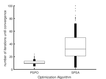
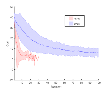
where, w𝑤w is a Gaussian noise w𝒩(0,32)similar-to𝑤𝒩0superscript32w\sim\mathcal{N}(0,3^{2}). This convex objective function is suitable for comparison of different optimizers without worrying about local minimum issues. We rerun each optimization algorithm 200200200 times for different initial conditions. According to Fig. 1a, we found that the PSPO algorithm converges faster than SPSA on average. Note that the maximum number of iteration set to 100100100 for both algorithms. The efficiency of the two algorithms is also tested through running the algorithms for a fixed initial condition many times. Fig. 1b shows the result. In this example, the number of function evaluations per iteration for the PSPO algorithm is twice of the number of function evaluations per iteration for the SPSA algorithm. But, as it can be seen in Fig. 1b, in case we have access to supercomputers to run the stochastic simulations in parallel, then the PSPO algorithm converges faster.
Refer to caption
(a)
Refer to caption
(b)
Figure 1. Comparison of SPSA and PSPO on optimization of a noisy convex objective function. (a) Number of iterations to converge. (b) Incremental decrease of objective function for two algorithms.

4.2. Real Application: Epidemiological Model Calibration

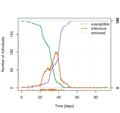
To demonstrate the efficiency of the PSPO algorithm proposed in this paper, we implemented the methodology on a data set concerns a measles outbreak in a small town in Germany in 1861, which contains 188 infected individuals. This data set, called Hagelloch data set, is very popular in literature because of its completeness and depth of data. Fig. 2 gives the observed clinical data. The data are obtained from (Meyer et al., 2014). The objective, here, is finding a good model for the given epidemic data to investigate the properties of the disease spread. To estimate the model parameters, we use maximum likelihood estimate (MLE). Details on how we can formulate this problem as an optimization problem can be found in (Alaeddini and Klein, 2017).
Refer to caption
Figure 2. Measles outbreak clinical data. The orange solid line, green dashed line, and dotted blue line represent the number of infected, susceptible, and recovered people respectively.

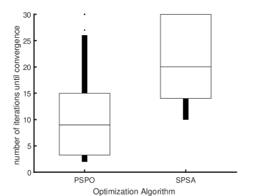
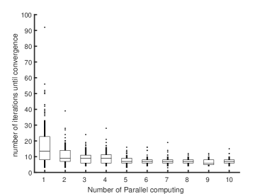
We compare the efficiency of the PSPO algorithm with the conventional SPSA algorithm. To compare these two algorithms, we rerun each optimization algorithms 100 times. Fig. 3a shows the number of iterations required to converge. As it can be seen in this figure, PSPO algorithm on average needs fewer iterations compared with the conventional SPSA algorithm. The maximum number of iterations for both algorithms set to 30. Note that the number of iterations until convergence set to 30 if the algorithm does not converge after 30 iterations. In order to investigate the performance of the PSPO algorithm as the number of parallel rounds increases, we run the PSPO for this example with different number of parallel computation rounds. Fig. 3b shows the number of iterations for convergence as M𝑀M grows. In this example, again, the number of function evaluations per iteration for the PSPO is twice of the corresponding number for the SPSA algorithm. Having higher number of function evaluations per iteration in this example, we can still see in Fig. 3a that the number of total function evaluations for PSPO might be less than the total number of function evaluations for SPSA. However, in this paper we do not focus on reducing the number of objective function evaluations and only focus on the faster convergence in case of having access to parallel supercomputers.
Refer to caption
(a)
Refer to caption
(b)
Figure 3. (a) Comparison of the number of iterations for convergence for conventional SPSA and PSPO. (b) Number of iterations vs. number of parallel computing rounds, M𝑀M, in PSPO.

5. Conclusions

In many stochastic optimization problems that noise presents, obtaining an analytical solution is hardly possible. In this paper, we described an algorithm for optimal parameter estimation in discretely observed stochastic model. We have introduced PSPO, which is a simple and computationally efficient algorithm for gradient-based optimization of stochastic objective functions. The comparison between SPSA and PSPO algorithm demonstrated the superiority of the PSPO algorithm in the number of iterations for convergence. Note that, comparing with SPSA, the PSPO algorithm with multiple parallel computations requires additional function evaluations per iteration. In case that we do not have access to powerful parallel computers, in order to prevent unnecessary long processing time per iteration, which results in long total processing time, the number of parallel computations need to be carefully computed using the level of the noise presented in the problem. We found the minimum number of parallel rounds of computation in order to have a bounded error in the estimated gradient. In some cases when we are dealing with a high SNR (signal to noise ratio) problem, a single round of computation might be enough for convergence, but in some other applications that the data are highly noisy the SPSA algorithm requires too many iterations to converge or even diverges. Our method is aimed towards highly uncertain objective functions.

Acknowledgements.
The authors thank Bill and Melinda Gates for their active support of this work and their sponsorship through the Global Good Fund. This work was performed at Institute for Disease Modeling with help from colleagues, especially Philip Eckhoff.

References

  • (1)
  • Alaeddini and Klein (2017) Atiye Alaeddini and Daniel J. Klein. 2017. Application of a second-order stochastic optimization algorithm for fitting stochastic epidemiological models. 2017 Winter Simulation Conference (WSC) (Dec 2017), 2194–2206.
  • Bhatnagar et al. (2003) Shalabh Bhatnagar, Michael C Fu, Steven I Marcus, I Wang, et al. 2003. Two-timescale simultaneous perturbation stochastic approximation using deterministic perturbation sequences. ACM Transactions on Modeling and Computer Simulation (TOMACS) 13, 2 (2003), 180–209.
  • Byrd et al. (2011) Richard H Byrd, Gillian M Chin, Will Neveitt, and Jorge Nocedal. 2011. On the use of stochastic hessian information in optimization methods for machine learning. SIAM Journal on Optimization 21, 3 (2011), 977–995.
  • Fröberg (1969) Carl-Erik Fröberg. 1969. Introduction to numerical analysis. Addison-Wesley Publishing Company Reading Massachusetts.
  • Fu (1994) Michael C Fu. 1994. Optimization via simulation: A review. Annals of operations research 53, 1 (1994), 199–247.
  • Hong and Nelson (2009) L Jeff Hong and Barry L Nelson. 2009. A brief introduction to optimization via simulation. In Proceedings of the 2009 Winter Simulation Conference (WSC). Institute of Electrical and Electronics Engineers, Inc., Piscataway, New Jersey, 75–85.
  • Kiefer et al. (1952) Jack Kiefer, Jacob Wolfowitz, et al. 1952. Stochastic estimation of the maximum of a regression function. The Annals of Mathematical Statistics 23, 3 (1952), 462–466.
  • Kocsis and Szepesvári (2006) Levente Kocsis and Csaba Szepesvári. 2006. Universal parameter optimisation in games based on SPSA. Machine learning 63, 3 (2006), 249–286.
  • Ma et al. (2013) Jingtao Ma, Yu Marco Nie, and H Michael Zhang. 2013. Solving the integrated corridor control problem using simultaneous perturbation stochastic approximation. In Advances in Dynamic Network Modeling in Complex Transportation Systems. Springer, 89–113.
  • Meyer et al. (2014) Sebastian Meyer, Leonhard Held, and Michael Höhle. 2014. Spatio-temporal analysis of epidemic phenomena using the R package surveillance. arXiv preprint arXiv:1411.0416 (2014).
  • Polyak and Juditsky (1992) Boris T Polyak and Anatoli B Juditsky. 1992. Acceleration of stochastic approximation by averaging. SIAM Journal on Control and Optimization 30, 4 (1992), 838–855.
  • Robbins and Monro (1951) Herbert Robbins and Sutton Monro. 1951. A stochastic approximation method. The annals of mathematical statistics (1951), 400–407.
  • Rumelhart et al. (1985) David E Rumelhart, Geoffrey E Hinton, and Ronald J Williams. 1985. Learning internal representations by error propagation. Technical Report. DTIC Document.
  • Spall (1992) James C Spall. 1992. Multivariate stochastic approximation using a simultaneous perturbation gradient approximation. IEEE transactions on automatic control 37, 3 (1992), 332–341.
  • Spall (2000) James C Spall. 2000. Adaptive stochastic approximation by the simultaneous perturbation method. IEEE transactions on automatic control 45, 10 (2000), 1839–1853.
  • Spall (2009) James C Spall. 2009. Feedback and weighting mechanisms for improving Jacobian estimates in the adaptive simultaneous perturbation algorithm. IEEE Trans. Automat. Control 54, 6 (2009), 1216–1229.
  • Swisher et al. (2000) James R Swisher, Paul D Hyden, Sheldon H Jacobson, and Lee W Schruben. 2000. A survey of simulation optimization techniques and procedures. In Proceedings of Winter Simulation Conference, Vol. 1. Institute of Electrical and Electronics Engineers, Inc., Piscataway, New Jersey, 119–128.
  • Tsilifis et al. (2017) Panagiotis Tsilifis, Roger G Ghanem, and Paris Hajali. 2017. Efficient bayesian experimentation using an expected information gain lower bound. SIAM/ASA Journal on Uncertainty Quantification 5, 1 (2017), 30–62.
  • Wright and Nocedal (1999) SJ Wright and J Nocedal. 1999. Numerical optimization. Vol. 2. Springer New York.

Appendix

Proof of Lemma 3.5

See 3.5

Proof.

We know that the Hessian matrix H𝐻H of f𝑓f is a square n×n𝑛𝑛n\times n matrix, defined as follows:

(15) H=[2f𝐱122f𝐱1𝐱22f𝐱1𝐱n2f𝐱1𝐱22f𝐱222f𝐱2𝐱n2f𝐱1𝐱n2f𝐱2𝐱n2f𝐱n2]=[𝐠1𝐱𝐠2𝐱𝐠n𝐱],𝐻matrixsuperscript2𝑓superscriptsubscript𝐱12superscript2𝑓subscript𝐱1subscript𝐱2superscript2𝑓subscript𝐱1subscript𝐱𝑛superscript2𝑓subscript𝐱1subscript𝐱2superscript2𝑓superscriptsubscript𝐱22superscript2𝑓subscript𝐱2subscript𝐱𝑛superscript2𝑓subscript𝐱1subscript𝐱𝑛superscript2𝑓subscript𝐱2subscript𝐱𝑛superscript2𝑓superscriptsubscript𝐱𝑛2matrixsubscript𝐠1𝐱subscript𝐠2𝐱subscript𝐠𝑛𝐱H=\begin{bmatrix}\frac{\partial^{2}f}{\partial\mathbf{x}_{1}^{2}}&\frac{\partial^{2}f}{\partial\mathbf{x}_{1}\partial\mathbf{x}_{2}}&\ldots&\frac{\partial^{2}f}{\partial\mathbf{x}_{1}\partial\mathbf{x}_{n}}\\ \frac{\partial^{2}f}{\partial\mathbf{x}_{1}\partial\mathbf{x}_{2}}&\frac{\partial^{2}f}{\partial\mathbf{x}_{2}^{2}}&\ldots&\frac{\partial^{2}f}{\partial\mathbf{x}_{2}\partial\mathbf{x}_{n}}\\ \vdots&\vdots&\ddots&\vdots\\ \frac{\partial^{2}f}{\partial\mathbf{x}_{1}\partial\mathbf{x}_{n}}&\frac{\partial^{2}f}{\partial\mathbf{x}_{2}\partial\mathbf{x}_{n}}&\ldots&\frac{\partial^{2}f}{\partial\mathbf{x}_{n}^{2}}\end{bmatrix}=\begin{bmatrix}\frac{\partial\mathbf{g}_{1}}{\partial\mathbf{x}}\\ \frac{\partial\mathbf{g}_{2}}{\partial\mathbf{x}}\\ \vdots\\ \frac{\partial\mathbf{g}_{n}}{\partial\mathbf{x}}\end{bmatrix}\,,

where 𝐠isubscript𝐠𝑖\mathbf{g}_{i} is the value of the gradient in 𝐞isubscript𝐞𝑖\mathbf{e}_{i} direction, and can be approximated by

𝐠i=𝐠T𝐞ij=1nf(𝐱+𝐝j)f(𝐱)𝐝j2𝐝jT𝐞i.subscript𝐠𝑖superscript𝐠𝑇subscript𝐞𝑖superscriptsubscript𝑗1𝑛𝑓𝐱subscript𝐝𝑗𝑓𝐱superscriptnormsubscript𝐝𝑗2superscriptsubscript𝐝𝑗𝑇subscript𝐞𝑖\mathbf{g}_{i}=\mathbf{g}^{T}\mathbf{e}_{i}\approx\sum_{j=1}^{n}\frac{f(\mathbf{x}+\mathbf{d}_{j})-f(\mathbf{x})}{\|\mathbf{d}_{j}\|^{2}}\mathbf{d}_{j}^{T}\mathbf{e}_{i}\,.

The full gradient of 𝐠isubscript𝐠𝑖\mathbf{g}_{i} can also be approximated using the finite difference method as follows:

𝐠i𝐱j=1n𝐠i(𝐱+𝐝j)𝐠i(𝐱)𝐝j2𝐝jT.subscript𝐠𝑖𝐱superscriptsubscript𝑗1𝑛subscript𝐠𝑖𝐱subscript𝐝𝑗subscript𝐠𝑖𝐱superscriptnormsubscript𝐝𝑗2superscriptsubscript𝐝𝑗𝑇\frac{\partial\mathbf{g}_{i}}{\partial\mathbf{x}}\approx\sum_{j=1}^{n}\frac{\mathbf{g}_{i}(\mathbf{x}+\mathbf{d}_{j})-\mathbf{g}_{i}(\mathbf{x})}{\|\mathbf{d}_{j}\|^{2}}\mathbf{d}_{j}^{T}\,.

Now, (15) can be written as

(16) H=[𝐠1𝐱𝐠2𝐱𝐠n𝐱][j=1n𝐠1(𝐱+𝐝j)𝐠1(𝐱)𝐝j2𝐝jTj=1n𝐠2(𝐱+𝐝j)𝐠2(𝐱)𝐝j2𝐝jTj=1n𝐠n(𝐱+𝐝j)𝐠n(𝐱)𝐝j2𝐝jT]=j=1n[𝐠1(𝐱+𝐝j)𝐠1(𝐱)𝐠2(𝐱+𝐝j)𝐠2(𝐱)𝐠n(𝐱+𝐝j)𝐠n(𝐱)]𝐝jT𝐝j2.𝐻matrixsubscript𝐠1𝐱subscript𝐠2𝐱subscript𝐠𝑛𝐱matrixsuperscriptsubscript𝑗1𝑛subscript𝐠1𝐱subscript𝐝𝑗subscript𝐠1𝐱superscriptnormsubscript𝐝𝑗2superscriptsubscript𝐝𝑗𝑇superscriptsubscript𝑗1𝑛subscript𝐠2𝐱subscript𝐝𝑗subscript𝐠2𝐱superscriptnormsubscript𝐝𝑗2superscriptsubscript𝐝𝑗𝑇superscriptsubscript𝑗1𝑛subscript𝐠𝑛𝐱subscript𝐝𝑗subscript𝐠𝑛𝐱superscriptnormsubscript𝐝𝑗2superscriptsubscript𝐝𝑗𝑇superscriptsubscript𝑗1𝑛matrixsubscript𝐠1𝐱subscript𝐝𝑗subscript𝐠1𝐱subscript𝐠2𝐱subscript𝐝𝑗subscript𝐠2𝐱subscript𝐠𝑛𝐱subscript𝐝𝑗subscript𝐠𝑛𝐱superscriptsubscript𝐝𝑗𝑇superscriptnormsubscript𝐝𝑗2\displaystyle H=\begin{bmatrix}\frac{\partial\mathbf{g}_{1}}{\partial\mathbf{x}}\\ \frac{\partial\mathbf{g}_{2}}{\partial\mathbf{x}}\\ \vdots\\ \frac{\partial\mathbf{g}_{n}}{\partial\mathbf{x}}\end{bmatrix}\approx\begin{bmatrix}\sum_{j=1}^{n}\frac{\mathbf{g}_{1}(\mathbf{x}+\mathbf{d}_{j})-\mathbf{g}_{1}(\mathbf{x})}{\|\mathbf{d}_{j}\|^{2}}\mathbf{d}_{j}^{T}\\ \sum_{j=1}^{n}\frac{\mathbf{g}_{2}(\mathbf{x}+\mathbf{d}_{j})-\mathbf{g}_{2}(\mathbf{x})}{\|\mathbf{d}_{j}\|^{2}}\mathbf{d}_{j}^{T}\\ \vdots\\ \sum_{j=1}^{n}\frac{\mathbf{g}_{n}(\mathbf{x}+\mathbf{d}_{j})-\mathbf{g}_{n}(\mathbf{x})}{\|\mathbf{d}_{j}\|^{2}}\mathbf{d}_{j}^{T}\end{bmatrix}=\sum_{j=1}^{n}\begin{bmatrix}\mathbf{g}_{1}(\mathbf{x}+\mathbf{d}_{j})-\mathbf{g}_{1}(\mathbf{x})\\ \mathbf{g}_{2}(\mathbf{x}+\mathbf{d}_{j})-\mathbf{g}_{2}(\mathbf{x})\\ \vdots\\ \mathbf{g}_{n}(\mathbf{x}+\mathbf{d}_{j})-\mathbf{g}_{n}(\mathbf{x})\end{bmatrix}\frac{\mathbf{d}_{j}^{T}}{\|\mathbf{d}_{j}\|^{2}}\,.

Thus

Hj=1n𝐠(𝐱+𝐝j)𝐠(𝐱)𝐝j2𝐝jT=i=1nΔGi𝐝i2𝐝iT.𝐻superscriptsubscript𝑗1𝑛𝐠𝐱subscript𝐝𝑗𝐠𝐱superscriptnormsubscript𝐝𝑗2superscriptsubscript𝐝𝑗𝑇superscriptsubscript𝑖1𝑛Δsubscript𝐺𝑖superscriptnormsubscript𝐝𝑖2superscriptsubscript𝐝𝑖𝑇H\approx\sum_{j=1}^{n}\frac{\mathbf{g}(\mathbf{x}+\mathbf{d}_{j})-\mathbf{g}(\mathbf{x})}{\|\mathbf{d}_{j}\|^{2}}\mathbf{d}_{j}^{T}=\sum_{i=1}^{n}\frac{\Delta G_{i}}{\|\mathbf{d}_{i}\|^{2}}\mathbf{d}_{i}^{T}\,.