The Stochastic Processes Generation in OpenModelica

Abstract

Background

Component-based modeling language Modelica (OpenModelica is open source implementation) is used for the numerical simulation of complex processes of different nature represented by ODE system. However, in OpenModelica standard library there is no routines for pseudo-random numbers generation, which makes it impossible to use for stochastic modeling processes.

Purpose

The goal of this article is a brief overview of a number of algorithms for generation a sequence of uniformly distributed pseudo random numbers and quality assessment of the sequence given by them, as well as the ways to implement some of these algorithms in OpenModelica system.

Methods

All the algorithms are implemented in C language, and the results of their work tested using open source package DieHarder. For those algorithms that do not use bit operations, we describe there realisation using OpwnModelica. The other algorithms can be called in OpenModelica as C functions

Results

We have implemented and tested about nine algorithms. DieHarder testing revealed the highest quality pseudo-random number generators. Also we have reviewed libraries Noise and AdvancedNoise, who claim to be adding to the Modelica Standard Library.

Conclusions

In OpenModelica system can be implemented generators of uniformly distributed pseudo-random numbers, which is the first step towards to make OpenModelica suitable for simulation of stochastic processes.

I Introduction

In this article we study the problem of generation uniformly distributed pseudo-random numbers, stochastic Wiener and Poisson processes in OpenModelica framework L_OpenModelica . OpenModelica is one of the open source implementation of Modelica L_Modelica modeling language (for other implementations see L_SciLab ; L_LMS ; L_Dymola ; L_JModelica ; L_WolframSystemModeler ; L_MapleSim ). This language is designed for modeling various systems and processes that can be represented as a system of algebraic or differential equations. For the numerical solution of the equations OpenModelica uses a number of open source libraries L_lis:2016 ; L_LAPACK:2016 ; L_UMFPACK:2016 ; L_KINSOL:2015 . However, in OpenModelica standard library there is no any function even for generating uniformly distributed pseudo-random numbers.

The first part of the article provides an overview of some algorithms for generation pseudo-random numbers, including description of pseudo-device /dev/random of Unix OS. For most of them we provide the algorithm written in pseudocode. We implement all described algorithms in the language of C and partly in OpenModelica. Also we tested them with dieharder — a random number generator testing suite L_DieHarder:2013 .

In the second part of the paper we describe algorithms for generating normal and Poisson distributions. These algorithms are based on the generators of uniformly distributed pseudo-random numbers. Then we study the problem of computer generation of stochastic Wiener and Poisson processes .

The third part of the article has a practical focus and is devoted to the description of calling external functions, written in C language, directly from OpenModelica programs code.

II Algorithms for generating uniformly distributed pseudo-random numbers

In this section we will describe some of the most common generators of uniformly distributed pseudo-random numbers. These generators are the basis for obtaining a sequence of pseudo-random numbers of other distributions.

II.1 Linear congruential generator

A linear congruential generator (LCG) was first proposed in 1949 by D. H. Lehmer L_DKnuth:1997:en . The algorithm 1 is given by formula:

$$x_{n+1}=(ax_{n}+c)\mod m,\;\;n\geqslant 0,$$

where $m$ is the mask or the modulus $m>1$, $a$ is the multiplier $(0\leqslant a<m)$, $c$ is the increment $(0\leqslant c<m)$, $x_{0}$ is the seed or initial value. The result of the repeated application of this recurrence formula is linear congruential sequence $x_{1},\ldots,x_{n}$. A special case $c=0$ is called multiplicative congruential method.

Algorithm 1 LCG — linear congruential generator

$n$, $seed$

$\mathrm{const}\;\;m\leftarrow 2^{64}$

$\mathrm{const}\;\;a\leftarrow 6364136223846793005$

$\mathrm{const}\;\;c\leftarrow 1442695040888963407$

$x_{0}\leftarrow seed$

for $i=0$ to $n$ do

     $x_{i}=(a\cdot x_{i-1}+c)\mod m$

end for

return $\{x_{0},x_{1},\ldots,x_{n}\}$

The number $m$, $a$, $c$ is called a <<magic>> or <<magic>> because their values are specified in the code of the program and are selected based on the experience of the use of the generator. The quality of the generated sequence depends essentially on the correct choice of these parameters. The sequence $\{x\}^{n}_{1}$ is periodic and its period depends on the number $m$, which must therefore be large. In practice, one chooses $m$ equal to the machine word size (for 32-bit architecture — $2^{32}$, for 64-bit architecture — $2^{64}$). D. Knuth L_DKnuth:1997:en recommends to choose

$$a=6364136223846793005,\;c=1442695040888963407,\;m=2^{64}=18446744073709551616.$$

In the article L_Ecuyer:1999 , you can find large tables with optimal values $a$, $b$ and $m$.

Also there are generalisations of LCG, such as quadratic congruential method $x_{n}=(ax_{n-1}^{2}+bx_{n-1}+d)\mod m$ cubic congruential method $x_{n}=(ax_{n-1}^{3}+bx_{n-1}^{2}+cx_{n-1}+d)\mod 2^{e}$.

Currently, the linear congruential method has mostly a historical value, as it generates relatively low-quality pseudo-random sequence compared to other, equally simple generators.

II.2 Lagged Fibonacci generator

The lagged Fibonacci generation can be considered as the generalization of the linear congruential generator. The main idea of this generalisation is to use multiple previous elements to generate current one. Knuth L_DKnuth:1997:en claims that the first such generator was proposed in the early 50-ies and based on the formula:

$$x_{n+1}=(x_{n}+x_{n-1})\mod m.$$

In practice, however, he showed himself not the best way. In 1958 George. J. Mitchell and D. Ph. Moore invented a much better generator 2

$$x_{n}=(x_{n-n_{a}}+x_{n-n_{b}})\mod m,\;n\geqslant\max(n_{a},n_{b}).$$

It was the generator that we now call LFG — lagged Fibonacci Generator.

Algorithm 2 LFG — Lagged Fibonacci generator

$n_{a}\leftarrow 55$

$n_{b}\leftarrow 24$

$s_{0},s_{1},\ldots,s_{n_{b}}$, $n\geqslant 0$

$x_{0},x_{1},\ldots,x_{n_{b}}$ $\leftarrow$ $r_{0},r_{1},\ldots,r_{n_{b}}$

for $i=(n_{a}+1)$ to $n$ do

     if $x_{i-n_{a}}\geqslant x_{i-n_{b}}$ then

         $x_{i}=x_{i-n_{a}}-x_{i-n_{b}}$

     else if $x_{i-n_{a}}<x_{i-n_{b}}$ then

         $x_{i}=x_{i-n_{a}}-x_{i-n_{b}}+1$

     end if

end for

return $\{x_{0},x_{1},\ldots,x_{n}\}$

As in the case of LCG generator <<magical numbers>> $n_{a}$ and $n_{b}$ greatly affects the quality of the generated sequence. The authors proposed to use the following magic numbers $n_{a}$ and $n_{b}$

$$n_{a}=24,n_{b}=55.$$

Knuth L_DKnuth:1997:en gives a number of other values, starting from $(37,100)$ and finishing with $(9739,23209)$. Period length of this generator is exactly equal to $2^{e-1}(2^{55}-1)$ when choosing $m=2^{e}$.

As can be seen from the algorithm for the initialization of this generator must be used one an initial value and a sequence of $\max(n_{a},n_{b})$ random numbers.

In open source GNU Scientific Library (GSL) L_GSL:2015 composite multi-recursive generator are used. It was proposed in paper L_Ecuyer:1996 . This generator is a generalisation of LFG may be expressed by the following formulas:

$$x_{n}=(a_{1}x_{n-1}+a_{2}x_{n-2}+a_{3}x_{n-3})\mod m_{1},$$

$$y_{n}=(b_{1}y_{n-1}+b_{2}y_{n-2}+b_{3}y_{n-3})\mod m_{2},$$

$$z_{n}=(x_{n}-y_{n})\mod m_{1}.$$

The composite nature of this algorithm allows to obtain a large period equal to $10^{56}\approx 2^{185}$. The GSL uses the following parameter values $a_{i},b_{i},m_{1},m_{2}$:

$$\begin{array}[]{lll}a_{1}=0,&b_{1}=86098,&m_{1}=2^{32}-1=2147483647,\\ a_{2}=63308,&b_{2}=0,&m_{2}=2145483479,\\ a_{3}=-183326,&b_{3}=-539608.&\end{array}$$

Another method suggested in the paper L_Ecuyer:1993:1 is also a kind of Fibonacci generator and is determined by the formula:

$$x_{n}=(a_{1}x_{n-1}+a_{5}x_{n-5})\mod 5,$$

The GSL used the following values: $a_{1}=107374182$, $a_{2}=0$, $a_{3}=0$, $a_{4}=0$, $a_{5}=104480$, $m=2^{31}-1=2147483647$. The period of this generator is equal to $10^{46}$.

II.3 Inversive congruential generator

Inverse congruential method based on the use of inverse modulo of a number.

$$x_{i+1}=(ax^{-1}_{i}+b)\mod m$$

where $a$ is multiplier $(0\leqslant a<n)$, $b$ is increment $(0\leqslant b<n)$, $x_{0}$ is initial value (seed). In addition $\text{GCD}(x_{0},m)=1$ and $\text{HCF}(a,m)=1$ is required.

This generator is superior to the usual linear method, however, is more complicated algorithmically, since it is necessary to find the inverse modulo integers which leads to performance reduction. To compute the inverse of the number usually applies the extended Euclidean algorithm (L_DKnuth:1997:en, , §4.3.2).

II.4 Generators with bitwise operations

Most generators that produce high quality pseudo-random numbers sequence use bitwise operations, such as conjunction, disjunction, negation, exclusive disjunction (xor) and bitwise right/left shifting.

II.4.1 Mersenne twister

Mersenne twister considered one of the best pseudo-random generators. It was developed in 1997 by Matsumoto and Nishimura L_Matsumoto:1998:MTE . There are 32-,64-,128-bit versions of the Mersenne twister. The name of the algorithm derives from the use of Mersenne primes $2^{19937}-1$. Depending on the implementation the period of this generator can be up to $2^{216091}-1$.

The main disadvantage of the algorithm is the relative complexity and, consequently, relatively slow performance. Otherwise, this generator provides high-quality pseudo-random sequence. An important advantage is the requirement of only one initiating number (seed). Mersenne twister is used in many standard libraries, for example in the Python 3 module random  L_Python3:3.5.1 .

Due to the complexity of the algorithm, we do not give its pseudocode in this article, however, the standard implementation of the algorithm created by Matsumoto and Nishimura freely available at the link http://www.math.sci.hiroshima-u.ac.jp/~m-mat/MT/emt64.html.

II.4.2 XorShift generator

Some simple generators (algorithms 3 and 4), giving a high quality pseudo-random sequence were developed in 2003 by George. Marsala (G. Marsaglia) L_xorshift:2003 ; L_xorshift:2005 .

$n$, $seed$

$x\leftarrow seed$

$y_{0}\leftarrow x$

for $i=1$ to $n$ do

     $x$ $\leftarrow$ $x\;\oplus$ $x\gg 12$

     $x$ $\leftarrow$ $x\;\oplus$ $x\ll 25$

     $x$ $\leftarrow$ $x\;\oplus$ $x\gg 27$

     $y_{i}\leftarrow x\cdot 2685821657736338717$

end for

return $\{y_{0},y_{1},\ldots,y_{n}\}$

Algorithm 3 xorshift*

Algorithm 4 xorshift+

$n$, $seed_{1}$, $seed_{2}$

for $i=1$ to $n$ do

     $x\leftarrow seed_{1}$

     $y\leftarrow seed_{2}$

     $seed_{1}\leftarrow y$

     $x=x\oplus(x<<23)$

     $seed_{2}=x\oplus y\oplus(x>>17)\oplus(y>>26)$

     $z_{i}\leftarrow seed_{2}+y$

end for

return $\{z_{1},\ldots,z_{n}\}$

II.4.3 KISS generator

Another group of generators (algorithms 5 and 6), giving a high quality sequence of pseudo-random numbers is KISS generators family L_KISS:2011 (Keep It Simple Stupid). They are used in the procedure random_number() of Frotran language (gfortran compiler L_gfortran:2015 )

$n$, $seed_{0},seed_{1},seed_{2},seed_{3}$

$t$

for $i=1$ to $n$ do

     $seed_{0}\leftarrow 69069\cdot seed_{0}+123456$

     $seed_{1}\leftarrow seed_{1}\oplus(seed_{1}<<13)$

     $seed_{1}\leftarrow seed_{1}\oplus(seed_{1}>>17)$

     $seed_{1}\leftarrow seed_{1}\oplus(seed_{1}<<5)$

     $t\leftarrow 698769069\cdot seed_{2}+seed_{3}$

     $seed_{3}\leftarrow(t>>32)$

     $seed_{1}\leftarrow t$

     $x_{i}\leftarrow seed_{0}+seed_{1}+seed_{2}$

end for

return $\{x_{1},\ldots,x_{n}\}$

Algorithm 5 KISS

$n$, $seed_{0},seed_{1},seed_{2},seed_{3}$

$t$

for $i=1$ to $n$ do

     $seed_{0}\leftarrow 314527869\cdot seed_{0}+1234567$

     $seed_{1}\leftarrow seed_{1}\oplus(seed_{1}<<5)$

     $seed_{1}\leftarrow seed_{1}\oplus(seed_{1}>>7)$

     $seed_{1}\leftarrow seed_{1}\oplus(seed_{1}<<22)$

     $t\leftarrow 4294584393\cdot seed_{2}+seed_{3}$

     $seed_{3}\leftarrow(t>>32)$

     $seed_{1}\leftarrow t$

     $x_{i}\leftarrow seed_{0}+seed_{1}+seed_{2}$

end for

return $\{x_{1},\ldots,x_{n}\}$

Algorithm 6 jKISS

II.5 Pseudo devices /dev/random and /dev/urandom

https://git.kernel.org/cgit/linux/kernel/git/stable/linux-stable.git/tree/drivers/char/random.c?id=refs/tags/v3.15.6#n52

To create a truly random sequence of numbers using a computer, some Unix systems (in particular GNU/Linux) uses the collection of <<background noise>> from the operating system environment and hardware. Source of this random noise are moments of time between keystrokes (inter-keyboard timings), various system interrupts and other events that meet two requirements: to be non-deterministic and be difficult for access and for measurement by external observer.

Randomness from these sources are added to an "entropy pool", which is mixed using a CRC-like function. When random bytes are requested by the system call, they are retrieved from the entropy pool by taking the SHA hash from it’s content. Taking the hash allows not to show the internal state of the pool. Thus the content restoration by hash computing is considered to be an impossible task. Additionally, the extraction procedure reduces the content pool size to prevent hash calculation for the entire pool and to minimize the theoretical possibility of determining its content.

External interface for the entropy pool is available as symbolic pseudo-device /dev/random, as well as the system function:

⬇

void get_random_bytes(void *buf, int nbytes);

% \end{minted}

The device /dev/random can be used to obtain high-quality random number sequences, however, it returns the number of bytes equal to the size of the accumulated entropy pool, so if one needs an unlimited number of random numbers, one should use a character pseudo-device /dev/urandom which does not have this restriction, but it also generates good pseudo-random numbers, sufficient for the most non-cryptographic tasks.

II.6 Algorithms testing

A review of quality criterias of an sequence of pseudo-random numbers can be found in the third chapter of the book L_DKnuth:1997:en , as well as in paper L_Ecuyer:2007 . All the algorithms, which we described in this articles, have been implemented in C-language and tested with Dieharder test suite, available on the official website L_DieHarder:2013 .

II.6.1 Dieharder overview

Dieharder is tests suite, which is implemented as a command-line utility that allows one to test a quality of sequence of uniformly distributed pseudorandom numbers. Also Dieharder can use any generator from GSL library L_GSL:2015 to generate numbers or for direct testing.

• dieharder -l — show the list of available tests,

• dieharder -g -1 — show the list of available random number generators; each generator has an ordinal number, which must be specified after -g option to activate the desired generator.

  • 200 stdin_input_raw — to read from standard input binary stream,

  • 201 file_input_raw — to read the file in binary format,

  • 202 file_input — to read the file in text format,

  • 500 /dev/random — to use a pseudo-device /dev/random,

  • 501 /dev/urandom — to use a pseudo-device /dev/urandom.

Each pseudorandom number should be on a new line, also in the first lines of the file one must specify: type of number (d — integer double-precision), the number of integers in the file and the length of numbers ($32$ or $64$ - bit). An example of such a file:

                type: d
                count: 5
                numbit: 64
                1343742658553450546
                16329942027498366702
                3111285719358198731
                2966160837142136004
                17179712607770735227

When such a file is created, you can pass it to dieharder

dieharder -a -g 202 -f file.in > file.out

where the flag -a denotes all built-in tests, and the flag -f specifies the file for analysis. The test results will be stored in file.out file.

II.6.2 Test results and conclusions

The generator	Fail	Weak	Pass
LCG	52	6	55
LCG2	51	8	54
LFG	0	2	111
ICG	0	6	107
KISS	0	3	110
jKISS	0	4	109
XorShift	0	4	109
XorShift+	0	2	111
XorShift*	0	2	111
Mersenne Twister	0	2	111
dev/urandom	0	2	111

The best generators with bitwise operations are xorshift*, xorshift+ and Mersenne Twister. They all give the sequence of the same quality. The algorithm of the Mersenne Twister, however, is far more cumbersome than xorshift* or xorshift+, thus, to generate large sequences is preferable to use xorshift* or xorshift+.

Among the generators which use bitwise operations the best result showed Lagged Fibonacci generator. The test gives results at the level of XorShift+ and Mersenne Twister. However, one has to set minimum 55 initial values to initialize this generator, thus it’s usefulness is reduced to a minimum. Inverse congruential generator shows slightly worse results, but requires only one number to initiate the algorithm.

III Generation of Wiener and Poisson processes

Let us consider the generation of normal and Poisson distributions. The choice of these two distributions is motivated by their key role in the theory of stochastic differential equations. The most General form of these equations uses two random processes: Wiener and Poisson L_Platen_Bruti . Wiener process allows to take into account the implicit stochasticity of the simulated system, and the Poisson process — external influence.

III.1 Generation of the uniformly distributed pseudo-random numbers from the unit interval

Generators of pseudo-random uniformly distributed numbers are the basis for other generators. However, most of the algorithms require a random number from the unit interval $[0,1]$, while the vast majority of generators of uniformly distributed pseudo-random numbers give a sequence from the interval $[0,m]$ where the number $m$ depends on the algorithm and the bitness of the operating system and processor.

To obtain the numbers from the unit interval one can proceed in two ways. First, one can normalize existing pseudo-random sequence by dividing each it’s element on the maximum element. This approach is guaranteed to give $1$ as a random number. However, this method is bad when a sequence of pseudo-random numbers is too large to fit into memory. In this case it is better to use the second method, namely, to divide each of the generated number by $m$.

III.2 Normal distribution generation

An algorithm for normal distributed numbers generation has been proposed in 1958 by George. Bux and P. E. R. Mueller L_BoxMuller:1958 and named in their honor Box-Muller transformation. The method is based on a simple transformation. This transformation is usually written in two formats:

• standard form (was introduce in the paper L_BoxMuller:1958 ),

• polar form (suggested by George Bell L_Bell:1968 and R. Knop L_Knop:1969 ).

Standard form. Let $x$ and $y$ are two independent, uniformly distributed pseudo-random numbers from the interval $(0,1)$, then numbers $z_{1}$ and $z_{2}$ are calculated according to the formula

$$z_{1}=\cos(2\pi y)\sqrt{-2\ln{x}},\;z_{2}=\sin(2\pi y)\sqrt{-2\ln{x}}$$

и are independent pseudo-random numbers distributed according to a standard normal law $\mathcal{N}(0,1)$ with expectation $\mu=0$ and the standard deviation $\sigma=1$.

Polar form. Let $x$ and $y$ — two independent, uniformly distributed pseudo-random numbers from the interval $[-1,1]$. Let us compute additional value $s=x^{2}+y^{2}$. If $s>1$ or $s=0$ then existing $x$ and $y$ values should be rejected and the next pair should be generated and checked. If $0<s\geqslant 1$ then the numbers $z_{1}$ and $z_{2}$ are calculated according to the formula

$$z_{1}=x\sqrt{\dfrac{-2\ln{s}}{s}},\;z_{2}=y\sqrt{\dfrac{-2\ln{s}}{s}}$$

and are independent random numbers distributed according to a standard normal law $\mathcal{N}(0,1)$.

For computer implementation is preferable to use a polar form, because in this case one has to calculate only single transcendental function $\ln$, while in standard case three transcendental functions ($\ln$, $\sin$ $\cos$) have to be calculated. An example of the algorithm shown in figure 2

To obtain a general normal distribution from the standard normal distribution, one can use the formula $Z=\sigma\cdot z+\mu$ where $z\sim\mathcal{N}(0,1)$, and $Z\sim\mathcal{N}(\mu,\sigma)$.

III.3 The generation of a Poisson distribution

To generate a Poisson distribution there is a wide variety of algorithms L_Devroye ; L_Ahrens:1974 ; L_Ahrens:1982 . The easiest was proposed by Knut L_DKnuth:1997:en . This algorithm 1 uses uniform pseudo-random number from the interval $[0,1]$ for it’s work. The algorithm’s output example is depicted on figure 2

Algorithm 1 The generator of the Poisson distribution

$seed$, $\lambda$

$\Lambda\leftarrow\exp(-\lambda)$, $k\leftarrow 0$, $p\leftarrow 1$, $u\leftarrow seed$

repeat

     $k\leftarrow k+1$

     $u\leftarrow rand(u)$ $\triangleright$ generation of uniformly distributed random number

     $p=p\cdot u$

until $p>\Lambda$

return $k-1$

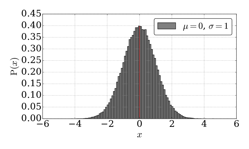
Figure 1: Normal distribution

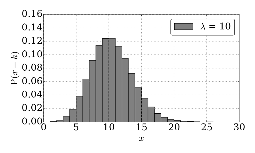
Figure 2: Poisson distribution

III.4 Generation of Poisson and Wiener processes

Now we going to use generators of normal and Poisson distributions to generate Wiener and Poisson stochastic processes. Let us first give the definition of these processes and then proceed to algorithms descriptions.

III.4.1 Definition of Wiener and Poisson stochastic processes

Let $(\Omega,\mathscr{A},P)$ — probability space, where $\Omega$ — the space of elementary events $\mathscr{A}$ — $\sigma$ - algebra of subsets of $\Omega$ (a random event), $P$ — the probability or probability measure, such that $P(\Omega)=1$.

A family of random variables $X=\{X_{t},0\leqslant t\leqslant T\}$, where $X_{t}\in\mathbb{R}^{d}$ will be called $d$–dimensional stochastic process, where a set of finite-dimensional distribution functions have the following properties (see L_Kloeden_Platen ; L_Oksendal_en )

$$F_{X_{t_{1}},X_{t_{2}},\ldots,X_{t_{k}}}(x_{i_{1}},x_{i_{2}},\ldots,x_{i_{k}})=P(X_{t_{1}}\leqslant x_{i_{1}},X_{t_{2}}\leqslant x_{i_{2}},\ldots,X_{t_{k}}\leqslant x_{i_{k}})$$

for all $i_{k}=1,2,3,\ldots$, $k=1,2,3,\ldots$, $x_{i}\in\mathbb{R}^{d}$ и $t_{k}\in\mathrm{T}$

The state space of $X$ is called $d$–dimensional Euclidean space $\mathbb{R}^{d}$, $d=1,2,3,\ldots$. The time interval $[0,T]$, where $T>0$. In numerical methods the sequence of time moments $\{t_{0},t_{1},t_{2},\ldots\}$ is used.

Random piecewise-constant process $N=\{N_{t},0\leqslant t\leqslant T\}$ with intensity $\lambda>0$ is called the Poisson process if the following properties are true (see L_Kloeden_Platen ; L_Oksendal_en ):

1. $P\{N_{0}=0\}=1$, otherwise $N_{0}=0$ almost surely.

2. $N_{t}$ has independent increments: $\{\Delta N_{0},\Delta N_{1},\ldots\}$ are independent random variables; $\Delta N_{t_{i}}=N_{t_{i+1}}-N_{t_{i}}$ and $0\leqslant t_{0}<t_{1}<t_{2}<\ldots<t_{n}\leqslant T$; $\Delta N_{t_{i}}=N_{t_{i+1}}-N_{t_{i}}$ и $0\leqslant t_{0}<t_{1}<t_{2}<\ldots<t_{n}\leqslant T$.

3. There is a number $\lambda>0$ such as, for any increment $\Delta N_{i},\;i=0,\ldots,n-1$, $E[\Delta N_{i}]=\lambda\Delta t_{i}$.

4. If $P(s)=P\{N_{t+s}-N_{t}>2\}$, then $\lim\limits_{s\to 0}\dfrac{P(s)}{s}=0$.

The random process $W=\{W_{t},0\leqslant t\leqslant T\}$ is called scalar Wiener process (Wiener) if the following conditions are true (see L_Kloeden_Platen ; L_Oksendal_en ).

1. $P\{W_{0}=0\}=1$, otherwise $W_{0}=0$ almost surely.

2. $W_{t}$ has independent increments: $\{\Delta W_{0},\Delta W_{1},\ldots\}$ are independent random variables; $\Delta W_{t_{i}}=W_{t_{i+1}}-W_{t_{i}}$ и $0\leqslant t_{0}<t_{1}<t_{2}<\ldots<t_{n}\leqslant T$.

3. $\Delta W_{i}=W_{t_{i+1}}-W_{t_{i}}\sim\mathcal{N}(0,t_{i+1}-t_{i})$ где $0\leqslant t_{i+1}<t_{i}<T$, $i=0,1,\ldots,n-1$.

From the definition it follows that $\Delta W_{i}$ is normally distributed random variable with expectation $\mathbb{E}[\Delta W_{i}]=\mu=0$ and variance $\mathbb{D}[\Delta W_{i}]=\sigma^{2}=\Delta t_{i}$.

Wiener process is a model of Brownian motion (the random walk). The process $W_{t}$ in following time points $0=t_{0}<t_{1}<t_{2}<\ldots<t_{N-1}<t_{N}$ experiences random additive changes: $W_{t_{1}}=W_{t_{0}}+\Delta W_{0},\;W_{t_{2}}=W_{t_{1}}+\Delta W_{1},\;\ldots,\;W(t_{N})=W(t_{N-1})+\Delta W_{n-1},$ where $\Delta W_{i}\sim\mathcal{N}(0,\Delta t_{i})$, $\forall i=0,\ldots,n-1$.

Let us write $W_{t_{n}}$ in the following form: $W_{t_{n}}=W_{t_{0}}+\sum\limits_{i=0}^{n-1}\Delta W_{i}$ and consider that $\mathbb{E}[\Delta W_{i}]=0$ and $\mathbb{D}[\Delta W_{i}]=\Delta t_{i}$. We can show now, that the sum of normally distributed random numbers $\Delta W_{i}$ is also normally distributed random number:

$$\mathbb{E}\sum\limits_{i=0}^{n-1}\Delta W_{i}=0,\;\;\mathbb{D}\sum\limits_{i=0}^{n-1}\Delta W_{i}=\sum\limits_{i=0}^{n-1}\Delta t_{i}=T,\;\;\sum\limits_{i=0}^{n-1}\Delta W_{i}\sim\mathcal{N}(0,T).$$

Multidimensional Wiener process $\mathbf{W}_{t}\colon\Omega\times[t_{0},T]\to\mathbb{R}^{m}$ is defined as a random process composed of jointly independent one-dimensional Wiener processes $W^{1}_{t},\ldots,W^{m}_{t}$. Increments $\Delta W^{\alpha}_{i},\;\forall\alpha=1,\ldots,m$ are jointly independent normal distributed random variables. On the other hand, the vector $\Delta W^{\alpha}_{i}$ can be represented as a multidimensional normally distributed random variable with expectation vector $\mu=1$ and a diagonal covariance matrix.

III.4.2 The generation of the Wiener process

To simulate one-dimensional Wiener process, one should generate the $N$ normally distributed random numbers $\varepsilon_{1},\ldots,\varepsilon_{N}$ and build their cumulative sums of $\varepsilon_{1}$, $\varepsilon_{1}+\varepsilon_{2}$, $\varepsilon_{1}+\varepsilon_{2}+\varepsilon_{3}$. As result we will get a trajectory of the Wiener process $W(t)$ cm Fig. 4.

In the case of multivariate random process, one needs to generate $m$ sequences of $N$ normally distributed random variables.

III.4.3 The generation of a Poisson process

A simulation of the Poisson process is much like Wiener one, but now we need to generate a sequence of numbers distributed according to the Poisson law and then calculate their cumulative sum. The plot of Poisson process is shown in Fig. 4. The figure shows that the Poisson process represents an abrupt change in numbers have occurred over time events. The intensity $\lambda$ depends on the average number of events over a period of time.

Because of this characteristic behavior of the Poisson process is also called an process with jumps and stochastic differential equations, with Poisson process as second driving process, are called equations with jumps L_Platen_Bruti

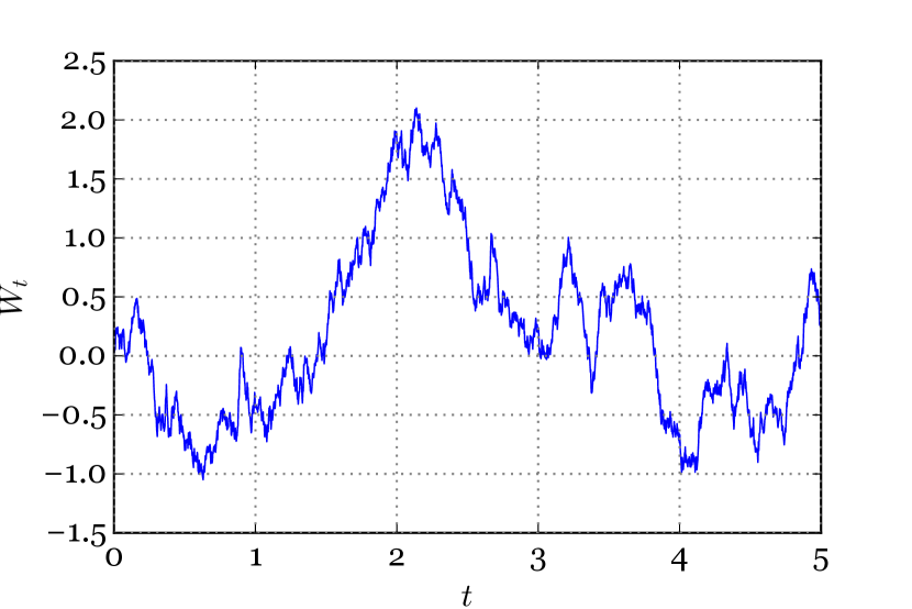
Figure 3: Wiener process

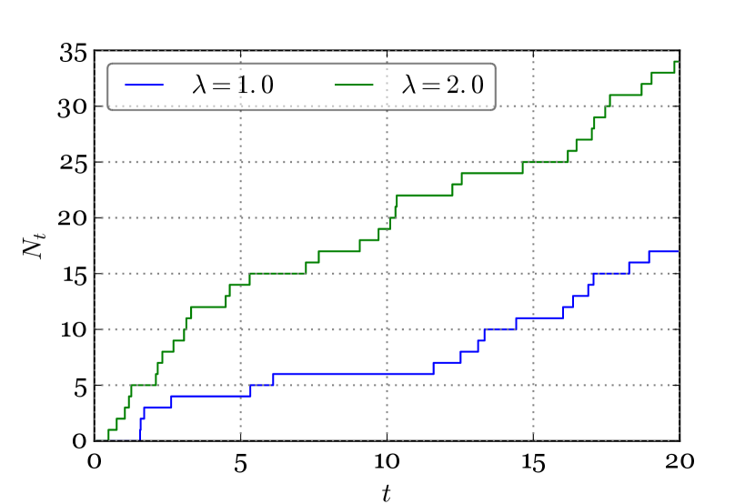
Figure 4: Poisson process

IV Simulation of stochastic processes in OpenModelica

As already mentioned in the introduction, there are no any pseudorandom numbers generators in OpenModelica. Thus that makes this system unusable for stochastic processes modeling. However Noise library build.openmodelica.org/Documentation/Noise.html developed by Klöckner (Klöckner) L_Klockner:2014 should be mentioned. The basis of this library are xorshift generators (algorithms 3 and 4), written in C. However, an inexperienced user may face a problem, because one needs compile C-source files first to use that library.

In this article we will describe the procedure required for connection of external C functions to OpenModelica programme. That will allow the user to install the Noise library and to connect their own random number generators. We also provide a minimal working example of stochastic Wiener process generator and the example of ordinary differential equation with additive stochastic part.

IV.1 Connection of external C-functions to OpenModelica program

Let us consider the process of connection of external functions to modelica program. The relevant section in the official documentation misses some essential steps that’s why it will lead to an error. All steps we described, had been performed on a computer with Linux Ubuntu 16.04 LTS and OpenModelica 1.11.0-dev-15.

When the code is compiled OpenModelica program is translated to C code that then is processed by C-compiler. Therefore, OpenModelica has built-in support of C-functions. In addition to the C language OpenModelica also supports Fortran (F77 only) and Python functions. However, both languages are supported indirectly, namely via wrapping them in the appropriate C-function.

The use of external C-functions may be required for various reasons, for example implementations of performance requiring components of the program, using a fullscale imperative programming language, or the use of existing sourcecode in C.

We give a simple example of calling C-functions from Modelica program. Let’s create two source files: ExternalFunc1.c and ExternalFunc2.c. These files will contain simple functions that we want to use in our Modelica program.

// File ExternalFunc1.c
double ExternalFunc1_ext(double x)
{
  return x+2.0*x*x;
}

// File ExternalFunc2.c
double ExternalFunc2(double x)
{
  return (x-1.0)*(x+2.0);;
}

In the directory, where the source code of Modelica program is placed, we must create two directories: Resources and the Library, which will contain ExternalFunc1.c and ExternalFunc2.c files. We should then create object files and place them in the archive, which will an external library. To do this we use the following command’s list:

gcc -c -o ExternalFunc1.o ExternalFunc1.c
gcc -c -o ExternalFunc2.o ExternalFunc2.c
ar rcs libExternalFunc1.a ExternalFunc1.o
ar rcs libExternalFunc2.a ExternalFunc2.o

To create object files, we use gcc with -c option and the archiver ar to place generated object files in the archive. As a result, we get two of the file libExternalFunc1.a and libExternalFunc2.a. There is also the possibility to put all the needed object files in a single archive.

To call external functions, we must use the keyword external. The name of the wrapper function in Modelica language can be differ from the name of the external function. In this case, we must explicitly specify which external functions should be wrapped.

model ExternalLibraries
        // Function name differs
  function ExternalFunc1
    input Real x;
    output Real y;
                // Explicitly specifying C-function name
                external y=ExternalFunc1_ext(x) annotation(Library="ExternalFunc1");
  end ExternalFunc1;

  function ExternalFunc2
    input Real x;
    output Real y;
                // The functions names are the same
                external "C" annotation(Library="ExternalFunc2");
  end ExternalFunc2;

  Real x(start=1.0, fixed=true), y(start=2.0, fixed=true);
equation
  der(x)=-ExternalFunc1(x);
  der(y)=-ExternalFunc2(y);
end ExternalLibraries;

Note that in the annotation the name of the external library is specified as ExternalFunc1, while the file itself is called libExternalFunc1.a. This is not a mistake and the prefix lib must be added to all library’s files.

The example shows that the type Real corresponds to the C type double. Additionally, the types of Integer and Boolean match the C-type int. Arrays of type Real and Integer transferred in arrays of type double and int.

It should be noted that consistently works only call с-functions with arguments of int and double types, as well as arrays of these types. The attempt to use specific c-type, for example, long long int or an unsigned type such as unsigned int, causes the error.

IV.2 Modeling stochastic Wiener process

Let us describe the implementation of a generator of the normal distribution and Wiener process. We assume that the generator of uniformly-distributed random numbers is already implemented in the functions urand. To generate the normal distribution we will use Box-Muller transformation and Wiener process can be calculated as cumulative sums of normally-distributed numbers.

The minimum working version of the code is shown below.The key point is the use of an operator sample(t_0, h), which generates events using h seconds starting from the time t_0. For every event the operator sample calls the function urand that returns a new random number.

  model generator
    Integer x1, x2;
    Port rnd; "Random number generator’s port"
    Port normal; "Normal numbers generator’s port"
    Port wiener; "Wiener process values port"
    Integer m = 429496729; "Generator modulo"
    Real u1, u2;
  initial equation
    x1 = 114561;
    x2 = 148166;
  algorithm
    when sample(0, 0.1) then
      x1 := urand(x1);
      x2 := urand(x2);
    end when;
    // normalisation of random sequence
    rnd.data[1] := x1 / m;
    rnd.data[2] := x2 / m;
    u1 := rnd.data[1];
    u2 := rnd.data[2];
    // normal generator
    normal.data[1] := sqrt(-2 * log(u1)) * sin(6.28 * u2);
    normal.data[2] := sqrt(-2 * log(u1)) * cos(6.28 * u2);
    // Wiener process
    wiener.data[1] := wiener.data[1] + normal.data[1];
    wiener.data[2] := wiener.data[2] + normal.data[2];
  end generator;

Note also the use of a special variable of type Port which serves to connect the various models together. In our example we have created three such variables: lg, normal, wiener. Because of this, other models can access the result of our generator.

  connector Port
    Real data[2];
  end Port;

A minimal working code below illustrates the connection example between two models. A system of two ordinary differential equations describes van der Pol–Duffing oscillator with additive stochastic part in the form of a Wiener process (see 5).

$$\left\{\begin{aligned} &\dot{x}=y,\\ &\dot{y}=x(1.0-x^{2})-y+x\cdot W_{t}.\end{aligned}\right.$$

It is important to mention that this equation is not stochastic. Built-in OpenModelica numerical methods do not allow to solve stochastic differential equations.

// the model specifies a system of ODE
  model ODE
    Real x, y;
    Port IN;
  initial equation
    x = 2.0;
    y = 0.0;
  equation
    der(x) = y ;
    der(y) = x*(1-x*x) - y + x*IN.data[1];
  end ODE;
  model sim
    generator gen;
    ODE eq;
  equation
    connect(gen.wiener, eq.IN);
  end sim;

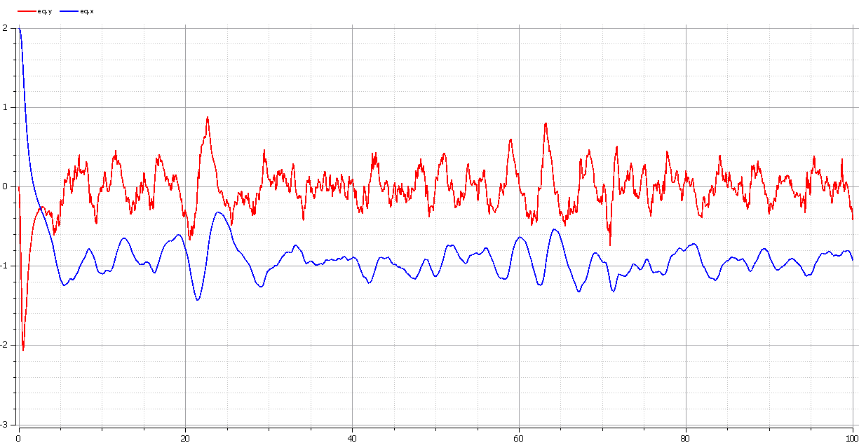
Figure 5: Results of van der Pol–Duffing oscillator simulation. The graphs are created using the functionality OMEditor’a

V Conclusion

We reviewed the basic algorithms for generating uniformly distributed pseudo-random numbers. All algorithms were implemented by the authors in C language and tested using DieHarder utility. The test results revealed that the most effective algorithms are xorshift and Mersenne Twister algorithms.

Due to the fact that OpenModelica does not implement bitwise logical and shifting operators, generators of uniformly distributed pseudo-random numbers have to be implemented in C language and connected to the program as external functions. We gave a rather detailed description of this process, that, as we hope, will fill a gap in the official documentation.