Concept of a next-generation electromagnetic phase-shift flowmeter for liquid metals

Abstract

We present a concept of an electromagnetic phase-shift flowmeter that has a significantly reduced sensitivity to the variation of the electrical conductivity of a liquid metal. A simple theoretical model of the flowmeter is considered where the flow is approximated by a solid finite-thickness conducting layer which moves in the presence of an ac magnetic field. In contrast to the original design [Priede et al., Meas. Sci. Technol. 22 (2011) 055402], where the flow rate is determined by measuring only the phase shift between the voltages induced in two receiving coils, the improved design measures also the phase shift between the sending and the upstream receiving coils. These two phase shifts are referred to as internal and external ones, respectively. We show that the effect of electrical conductivity on the internal phase shift, which is induced by the flow, can be strongly reduced by rescaling it with the external phase shift, which depends mostly on the conductivity of medium. Two different rescalings are found depending on the ac frequency. At low frequencies, when the shielding effect is weak, the effect of conductivity is strongly reduced by rescaling the internal phase shift with the external one squared. At higher frequencies, the same is achieved by rescaling the internal phase shift directly with the external one.

1 Introduction

Electromagnetic flow metering based on the voltage induced between the electrodes in contact with a conductive liquid that flows in the presence of magnetic field is a well established technique which works reliably for common liquids with conductivities as low as that of tap water, i.e., a few $\mathrm{\mu S/cm}$ [1]. Application of this standard technique to liquid metals is however hampered by various contact problems ranging from the corrosion of electrodes to spurious electrochemical and thermoelectric potentials [2]. The effect of spurious potentials can be mitigated by using a pulsed magnetic field [3]. The corrosion problem could in principle be avoided by using capacitately-coupled electrodes to measure the induced voltage in a contactless way [4, 5].

There are several more widely used contactless flow metering methods for liquid metals which rely on the eddy currents induced by the flow. As first suggested by Shercliff [6] and later pursued by the so-called Lorentz Force Velocimetry [7], the flow rate can be determined by measuring the force generated by eddy currents on a magnet placed close to the pipe carrying a conducting liquid. An alternative approach, which is virtually force-free and thus largely independent of the conductivity of liquid metal [8], is to determine the flow rate from the equilibrium rotation rate of a freely rotating magnetic flywheel [9, 10, 11] or just a single magnet [12]. More common are the contactless eddy-current flow meters which measure the the flow-induced perturbation of an externally applied magnetic field [13, 14, 15]. The same principle is used also by the so-called flow tomography approach, where the spatial distribution of the induced magnetic field is analysed [16, 17].

The main challenge to the eddy current flowmetering is the weak induced magnetic field with a relative amplitude of the order of magnitude of the magnetic Reynolds number $\mathit{Rm}\sim 10^{-4}-10^{-1}$, which has to be measured in the presence of a much stronger external magnetic field. Although the background signal produced by the external magnetic field can be compensated by a proper arrangement of sending and receiving coils [18], this type of flow meter remains highly susceptible to small geometrical imperfections.

Much more robust to geometrical disturbances is the phase-shift induction flowmeter [1, 19, 20]. Instead of the usual voltage difference, this flowmeter measures the phase shift induced by the flow between the voltages in two receiver coils. Because the phase is determined by the amplitude ratio, it remains invariant when the amplitudes are perturbed in a similar way. The main remaining drawback of this flowmeter is the dependence of the flow-induced phase shift not only on the velocity but also on the conductivity of liquid metal.

The susceptibility to varying conductivity is a general problem which plagues not only eddy-current [21] but also the Lorentz force devices. While there are devices which can address this problem, such as, for example, the single magnet rotary flowmeter [12], the transient eddy-current flowmeter [22, 23, 24] or the time-of-flight Lorentz force flowmeters [25], they come with other drawbacks such as moving parts or complicated measurement schemes. For standard eddy-current flowmeters, the effect of conductivity can be compensated by normalizing the voltage difference between two sensing coils with the sum of the voltages [26]. However, it has to be noted that this compensation scheme works only at a certain optimal AC frequency which depends on the setup [27].

This paper is concerned with the development of a next-generation phase-shift flowmeter with a reduced dependence on the conductivity of liquid metal. The basic idea is that not only the eddy currents induced by the liquid flow but also those induced by the alternating magnetic field itself give rise to a phase shift in the induced magnetic field and the associated emf which is picked up by the sensor coils. The latter effect, which leads to a phase shift between the sending and receiving coils, depends on the conductivity of the liquid. Therefore, it may be used to compensate for the effect of conductivity on the flow-induced phase shift. The feasibility of such an approach is investigated using two simple theoretical models of the phase-shift flowmeter, where the flow is approximated by a solid body motion of a finite-thickness conducting layer.

The paper is organised as follows. Mathematical model and the basic equations describing the phase-shift flowmeter are briefly recalled in the next section. In Section 3 we present and discuss numerical results for two simple configurations of the applied magnetic field: the first in the form of a mono-harmonic standing wave and the second generated by a simple coil made of couple of straight wires placed above the layer. The paper is concluded by a summary in Section 4. Relevant mathematical details of solutions behind numerical results are provided in the Appendix.

2 Mathematical model

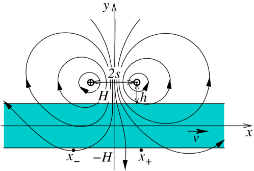
Figure 1: Sketch of the mathematical model of flowmeter consisting of an electrically conducting layer which moves as a solid body in the presence of alternating magnetic field generated by a couple of straight wires with opposite currents. Flow rate is determined by measuring the phase difference between the voltages induced in two sensor wires (coils) placed directly beneath the layer at the downstream and upstream horizontal positions $x_{-}$ and $x_{+},$ respectively.

Consider a layer of electrical conductivity $\sigma$ and thickness $2H$ which moves as a solid body with the velocity $\boldsymbol{v}=\boldsymbol{e}_{x}v$ in the presence of an alternating magnetic field $\boldsymbol{B}$ as shown in figure 1. The velocity profile as well as other technical details are ignored in this basic model whose main purpose to capture the key characteristics of flowmeter. The electric field induced by alternating magnetic field follows from the Maxwell-Faraday equation $\boldsymbol{E}=-\boldsymbol{\nabla}\Phi-\partial_{t}\boldsymbol{A},$ where $\Phi$ is the electric potential and $\boldsymbol{A}$ is the magnetic vector potential of the magnetic field $\boldsymbol{B}=\boldsymbol{\nabla}\times\boldsymbol{A}$. The electric current induced in the moving medium is given by Ohm’s law

$$\boldsymbol{j}=\sigma(\boldsymbol{E}+\boldsymbol{v}\times\boldsymbol{B})=\sigma(-\boldsymbol{\nabla}\Phi-\partial_{t}\boldsymbol{A}+\boldsymbol{v}\times\boldsymbol{\nabla}\times\boldsymbol{A}).$$

Subsequently, we consider a 2D magnetic field which is invariant in the $z$ direction (perpendicular to the plane of figure 1) and alternates in time harmonically with the angular frequency $\omega.$ Such a magnetic field, which has only two $(x$ and $y)$ components, is described by single $(z)$ component of the vector potential: $\boldsymbol{A}=\boldsymbol{e}_{z}A.$ In this case, we have $\boldsymbol{B}=-\boldsymbol{e}_{z}\times\boldsymbol{\nabla}A,$ which means $\boldsymbol{B}\cdot\boldsymbol{\nabla}A\equiv 0,$ i.e., the isolines of $A$ are the flux lines of $\boldsymbol{B}.$ A harmonically alternating solution can be found in the complex form as $A(\boldsymbol{r},t)=\Re\left[A(\boldsymbol{r})e^{\mathrm{i}\omega t}\right]$, where $A(\boldsymbol{r})$ is an amplitude distribution and $\boldsymbol{r}$ is the radius vector.

At sufficiently low alternation frequencies, which are typical for eddy current flowmeters, the displacement currents are negligible, and thus the Ampere’s law $\boldsymbol{j}=\mu_{0}^{-1}\boldsymbol{\nabla}\times\boldsymbol{B}$ leads to $\Phi\equiv 0.$ As a result, we obtain the following advection-diffusion equation for $A(\boldsymbol{r})$

$$\mu_{0}\sigma(\mathrm{i}\omega A+v\partial_{x}A)=\boldsymbol{\nabla}^{2}A,$$ (1)

where $\mu_{0}=4\pi\times 10^{-7}\,\mathrm{H/m}$ is the vacuum permeability. The continuity of $\boldsymbol{B}$ at the interface $S$ between the conducting medium and free space requires

$$\left[A\right]_{S}=\left[(\boldsymbol{n}\cdot\boldsymbol{\nabla})A\right]_{S}=0,$$ (2)

where $\left[\right]_{S}$ and $\boldsymbol{n}$ respectively denote a jump across $S$ and the unit normal to $S.$

In the following, we consider two basic configurations of the applied magnetic field [19]. The first is a mono-harmonic standing wave with the wave number $k$ in the $x$-direction

$$A_{0}(\boldsymbol{r},t)=\hat{A}_{0}(y)\cos(kx)\cos(\omega t).$$ (3)

The second is a magnetic field generated by an idealized finite-size coil which consists of two parallel straight wires carrying an ac current of amplitude $I_{0}$ that flows in opposite directions along the $z$-axis at distance $2s$ in the $x$-direction and the height $h$ above the upper surface of the layer, as shown in figure 1.

The two key parameters which appear in the problem are the dimensionless ac frequency $\bar{\omega}=\mu_{0}\sigma\omega H^{2}$ and the magnetic Reynolds number $\mathit{Rm}=\mu_{0}\sigma vH.$ The latter defines the velocity of layer in the units of the characteristic magnetic diffusion speed $(\mu_{0}\sigma H)^{-1}$ and is subsequently referred to as the dimensionless velocity. It is important to note that the dimensionless velocity defined in this way varies with the conductivity of medium. This variation is eliminated by taking the ratio $\mathit{Rm}/\bar{\omega}=v/(\omega H)\equiv\bar{v},$ which defines the velocity of layer relative to the characteristic phase speed of the magnetic field and is referred to as the relative velocity. For fixed $H$ and $\omega,$ the relative velocity depends only on the physical velocity $v,$ while $\bar{\omega}$ depends only on the conductivity of medium. Consequently, for the flowmeter to be insensitive to the conductivity variation of medium, its output signal should depend only on $\bar{v}$ but not on $\bar{\omega.}$

3 Results

3.1 Mono-harmonic magnetic field

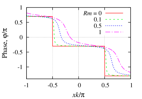
Figure 2: Phase distribution of the vector potential over a wavelength of the applied magnetic field along the bottom of the layer for $\bar{\omega}=1,$ $k=1$ and various dimensionless velocities $\mathit{Rm}.$

The problem formulated above has an analytical solution [19] which is used in the following. To make the paper self-contained, a summary of solution is provided in the Appendix.

We start with the external magnetic field in the form a mono-harmonic standing wave (3) and first briefly recall the basic characteristics of the original phase-shift flowmeter [19]. When the layer is at rest $(\mathit{Rm}=0),$ the induced magnetic field forms a standing wave like the external field. As the adjacent halves of standing wave oscillate in opposite phases, the phase distribution is piece-wise continuous along the wave. The phase of vector potential jumps by $\pi$ across the wave nodes, which for the $k=1$ shown in figure 2 are located at $x=\pm\pi/2.$ When the layer starts to move, the phase discontinuities are smoothed out and, with the increase of velocity, are shifted further downstream. As seen in figure 2, the strongest phase variation produced by the motion occurs just downstream of the wave nodes whilst the variation upstream remains relatively weak.

For the physical interpretation of these and subsequent results, note that the circulation of vector potential along a closed contour gives a magnetic flux through the encircled surface. For the 2D case under consideration, the vector potential has only one $(z)$ component $A$, and the difference of $A$ between two points defines the linear flux density between the two lines parallel to the vector potential at those two points. The same holds also for the time derivative of the corresponding quantities. Thus, the difference of the vector potential amplitudes between two points is proportional to the voltage amplitude measured by an idealised coil consisting of two straight parallel wires placed along the $z$-axis at those points. Correspondingly, the single-point vector potential gives the voltage measured by a ‘wide’ coil with the second wire placed sufficiently far away in the region of a negligible magnetic field.

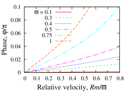
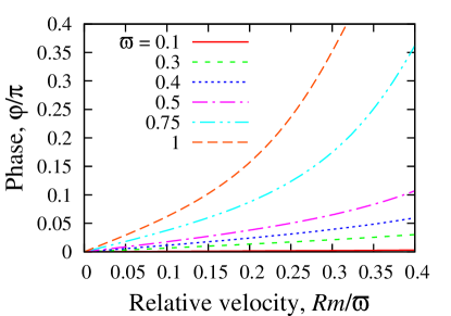
Figure 3: The phase shift $\Delta_{0}\varphi$ (scaled by $\pi)$ between two observation points placed below the layer at $\pm xk/\pi=0.2$ (a), $0.3$ (b) and $0.4$ (c) versus the relative velocity $\mathit{Rm}/\bar{\omega}$ for $k=1$ at various dimensionless frequencies $\bar{\omega}\lesssim 1.$

In the original concept, the flow rate is determined by measuring only the phase shift $\Delta_{0}\varphi$ between two observation points placed symmetrically with respect $x=0,$ which is the midpoint between two adjacent nodes of the mono-harmonic standing wave (3). The variation of this phase shift with the relative velocity $\bar{v}=v/(\omega H)$ is shown in figure 3 for various dimensionless ac frequencies $\bar{\omega},$ which correspond to various conductivities when the physical ac frequency $\omega$ is kept fixed. Since $\bar{v}$ is independent of the conductivity, the variation of $\Delta_{0}\varphi$ with $\bar{\omega}$ for a fixed $\omega$ is entirely due to the variation of conductivity. Since the flow-induced phase shift vanishes at low velocities, and according to Eq. (1) it does so directly with $\mathit{Rm},$ we have $\Delta_{0}\varphi\sim\mathit{Rm}$ for $\mathit{Rm}\ll 1.$ By the same arguments, for low ac frequencies, we have $\Delta_{0}\varphi\sim\bar{\omega.}$ For $\mathit{Rm}\ll 1$ and $\bar{\omega}\ll 1,$ the combination of these two relations imply a quadratic variation of the phase shift with the electrical conductivity of the medium:

$$\Delta_{0}\varphi\sim\bar{\omega}\mathit{Rm}\sim\sigma^{2}.$$ (4)

Our goal is to compensate the variation of the flow-induced phase shift with the conductivity by employing the information contained in the phase shift between the sending coil and one of the receiving coils. Namely, we shall use the phase shift between the sending and the upstream receiving coil, which is less affected by the motion of the conducting medium than the downstream one, to rescale the flow-induced phase shift between the voltages in the receiving coils.

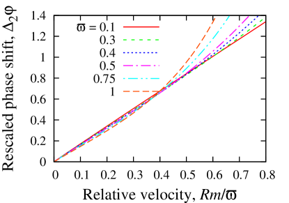
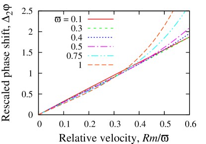
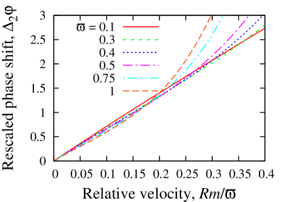
Figure 4: Rescaled phase shift $\Delta_{2}\varphi$ between two observation points placed below the layer at $\pm xk/\pi=0.2$ (a,b), $0.3$ (c,d) and $0.4$ (e,f) versus the relative velocity $\mathit{Rm}/\bar{\omega}$ for $k=1$ (a,c,e) and $k=0.5$ (b,d,f) at various dimensionless frequencies $\bar{\omega}\lesssim 1.$

Let us start with a low dimensionless frequency $\bar{\omega}\ll 1.$ In this case, the phase shift between sending and receiving coils, which we refer to as the external phase shift, and which is caused by the diffusion of the magnetic field through the conducting layer is expected to vary as $\varphi\sim\bar{\omega}$. This variation, which follows from the same arguments as Eq. (4), implies that the conductivity can be eliminated from the flow-induced phase shift (4) by the following rescaling

$$\Delta_{2}\varphi=\frac{\Delta_{0}\varphi}{\varphi_{-}^{2}},$$ (5)

where $\Delta_{0}\varphi=\varphi_{+}-\varphi_{-}$ is a difference between the phases of voltage, $\varphi_{+}$ and $\varphi_{-},$ measured at downstream and upstream observation points. For a fixed physical ac frequency, the variation of the dimensionless frequency $\bar{\omega}$ can be only due to by the variation of electrical conductivity which would cause also a variation of the dimensionless velocity $\mathit{Rm}$ independently of the variation of physical velocity. As discussed above, the quantity which varies with the physical velocity but not with the conductivity is the relative velocity $\bar{v}=\mathit{Rm}/\bar{\omega}.$ It means that in the ideal case of a perfectly compensated conductivity effect, the rescaled phase shift $\Delta_{2}\varphi$ should depend only on $\bar{v}$ but on $\bar{\omega.}$ Practically, we expect the rescaled phase shift to vary mostly with $\bar{v}$ and not so much with $\bar{\omega.}$ This can be seen to be the case for the rescaled phase shifts plotted in figure 4 which show a much weaker dependence on the dimensionless frequency than the unscaled phase shift shown in figure 3. For low relative velocities, the variation of rescaled phase shift with $\bar{\omega}$ remains rather weak up to $\bar{\omega}\sim 1,$ which is consistent with the original assumption of $\bar{\omega}\ll 1.$ The range of relative velocities which is weakly affected by $\bar{\omega}$ depends on the location of the observation points. The closer the observation points to the wave nodes $(xk/\pi=\pm 0.5),$ the shorter the range of the relative velocities for which $\Delta_{2}\varphi$ remains insensitive to the variation of $\bar{\omega}$. In this range of relative velocities, the increase of the dimensionless frequency from $0.1$ to $1,$ which is equivalent to the increase of the conductivity by an order of magnitude, results in a much smaller variation of the rescaled phase shift.

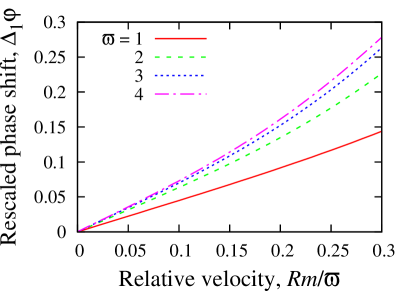
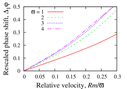
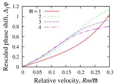
Figure 5: Rescaled phase shift $\Delta_{1}\varphi$ between two observation points placed below the layer at $\pm xk/\pi=0.2$ (a,b), $0.3$ (c,d) and $0.4$ (e,f) versus the relative velocity $\mathit{Rm}/\bar{\omega}$ for $k=1$ (a,c,e) and $k=0.5$ (b,d,f) at various dimensionless frequencies $\bar{\omega}\gtrsim 1.$

The above results show that rescaling (5) can compensate the effect of conductivity only at sufficiently low frequencies at which the variation of the frequency-induced (external) phase shift between the sending and receiving coils is close to linear with $\bar{\omega}.$ This scaling changes at higher frequencies when the shielding effect makes the variation of this phase shift non-linear with $\bar{\omega.}$ In this case, a new scaling can be deduced by the following order-of-magnitude arguments which will be confirmed by the subsequent numerical results.

For $\bar{\omega}\gg 1,$ a significant phase variation of order $\sim 1$ occurs in the conducting medium over the the characteristic skin layer thickness $\sim\bar{\omega}^{-1/2}.$ Consequently, the total phase shift due to the diffusion of the magnetic field through the whole conducting layer with the dimensionless thickness $\sim 1$ is expected to vary as $\varphi\sim\bar{\omega}^{1/2}\sim\sigma^{1/2}.$ On the other hand, since the applied magnetic field in the form of a standing wave consists of two oppositely travelling waves (see , Eq. (12) suggests that the motion of the layer is equivalent to the variation of the dimensionless frequency $\bar{\omega}$ by $k\mathit{Rm}\sim\mathit{Rm}\ll 1.$ Then the flow-induced phase shift between two receiving coils is expected to scale as

$$\Delta_{0}\varphi\sim\frac{\partial\varphi}{\partial\bar{\omega}}\mathit{Rm}\sim\bar{\omega}^{-1/2}\mathit{Rm}\sim\sigma^{1/2}.$$

This implies that for $\bar{\omega}\gtrsim 1$ the conductivity can be eliminated from the flow-induced phase shift between the receiving coils by rescaling it directly with the external phase shift as

$$\Delta_{1}\varphi=\frac{\Delta_{0}\varphi}{\varphi_{-}}.$$ (6)

The rescaled phase shift $\Delta_{1}\varphi$ is plotted in figure 5 against the relative velocity for two different wavenumbers $k=1$ and and $k=0.5$ and various dimensionless frequencies. For $k=1,$ the dependence of $\Delta_{1}\varphi$ on $\bar{\omega}$ is seen to diminish as the latter is increased above $1.$ For $k=0.5,$ which corresponds a wavelength of the applied magnetic field significantly larger than the thickness of the layer, the variation of $\Delta_{1}\varphi$ with $\bar{\omega}$ is practically insignificant starting from $\bar{\omega}\approx 1.$

3.2 External magnetic field generated by a pair of straight wires

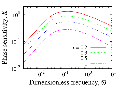
Figure 6: The phase sensitivity $K=\frac{1}{\pi}\left.\frac{\partial\varphi}{\partial\mathit{Rm}}\right|_{\mathit{Rm}=0}$ versus the dimensionless frequency $\bar{\omega}$ at various observation points at the bottom of the layer .

In this section, we consider a more realistic external magnetic field which is generated by a couple of parallel wires with opposite currents. The wires are separated by a horizontal distance of $2s=2$ and put at the height $h=1$ above the layer as shown in figure 1. For a layer at rest, the magnetic field distribution is mirror-symmetric with respect to the $x=0$ plane, which is analogous to a node in the mono-harmonic standing wave considered in the previous section. Correspondingly, when the layer is at rest, there is a phase jump of $\pi$ at $x=0.$ In contrast to the previous case, the phase is no longer constant on either side of the discontinuity and varies horizontally as well as vertically [19]. As a result, the range of dimensionless frequency where the phase sensitivity $K=\frac{1}{\pi}\left.\frac{\partial\varphi}{\partial\mathit{Rm}}\right|_{\mathit{Rm}=0},$ which is plotted in figure 6, varies more or less linearly with $\bar{\omega}$ and, thus, rescaling (5) could be applicable, is relatively short and limited to $\bar{\omega}\lesssim 0.02.$ Therefore, at $\bar{\omega}\sim 1,$ which presents the main interest from a practical point of view, scaling (6) is expected to be applicable. The phase shift rescaled in this way is plotted in figure 7 against the relative velocity for several locations of the observation points and various dimensionless frequencies. As seen, $\Delta_{1}\varphi$ depends essentially on the relative velocity while its variation with $\bar{\omega}$ is relatively weak except for the largest separation of the observation points $x=\pm 2.5,$ which is shown in figure 7(d). This deterioration of the rescaling at larger separations of observation points is likely due to the horizontal variation of the external phase shift mentioned above.

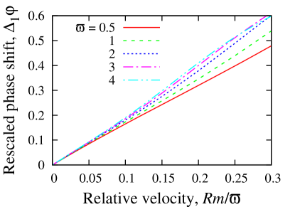
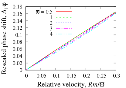
Figure 7: The rescaled phase shift $\Delta_{1}\varphi$ between two observation points placed below the layer at $\pm x=0.5$ (a), $1$ (b), $1.5$ (c), and $2.5$ (d) versus the relative velocity $\mathit{Rm}/\bar{\omega}$ at various dimensionless frequencies $\bar{\omega}.$

4 Summary and conclusion

We have presented a concept of an improved phase-shift flowmeter which is much less susceptible to the variations of electrical conductivity of liquid metal than the original design of Priede et al. [19]. In the improved flowmeter, we suggest to measure not only the phase shift between the voltages induced in two receiving coils, which is referred to as the internal phase shift, but also the external phase shift between the sending coil and the upstream receiving coil. In contrast to the internal phase shift, which is induced by the flow, the external one depends mostly on the conductivity of the media and not so much on its velocity. We rescale the internal phase shift with the external phase shift to eliminate, or at least strongly reduce, the effect of conductivity on the operation of the flowmeter. Two different rescalings are found depending on the ac frequency. At low frequencies $\bar{\omega}\lesssim 1,$ when the phase shift varies directly with the frequency, the conductivity can be eliminated by rescaling the internal phase shift with the square of the external phase shift. At higher ac frequencies $\bar{\omega}\gtrsim 1,$ where the shielding effect makes the variation of phase with the frequency non-linear, the conductivity can be eliminated by rescaling the internal phase shift directly with the external one. Note that for liquid sodium with $\sigma=8.3\times 10^{6}\,\mbox{S/m}$ [28] and characteristic size $H\sim 0.1\,\mathrm{m,}$ $\bar{\omega}\sim 1$ and $\mathit{Rm}\sim 1$ correspond to ac frequency $f\sim 60\,\mathrm{Hz}$ and velocity $v\sim 1\,\mathrm{m/s,}$ respectively.

The applicability of the first rescaling is limited to relatively low frequencies $(\bar{\omega}\ll 1)$, especially for realistic sending coils which generate the magnetic field dominated by long-wave harmonics. A potential disadvantage of using low ac frequencies may be the relatively low sensitivity of the phase-shift flowmeter. From this point of view, it seems more attractive to operate the flowmeter in the frequency range with a moderate shielding effect, i.e. with $\bar{\omega}\sim 1,$ where the second (direct) rescaling is applicable. Although rescaling can render the phase-shift flowmeter virtually insensitive to the conductivity variation of liquid metal, the flowmeter still requires calibration because the output signal is not related straightforwardly with the flow velocity as in the transient eddy- current [22, 23, 24] and the time-of-flight Lorentz force [25] flowmeters. The proposed concept can be used for designing a next-generation phase-shift flowmeter with increased robustness to the variations of the electrical conductivity of liquid metal, which may be required in some metallurgical and other applications.

5 Appendix

5.1 Analytical solution for mono-harmonic external magnetic field

The amplitude distribution of the external magnetic (3) in the free space, which follows from equation (1) with $\sigma=0$, can be written as

$$\hat{A}_{0}(y;k)=C_{0}e^{|k|(y-1)},$$ (7)

where the constant

$$C_{0}=\hat{A}_{0}(1;k)$$ (8)

defines the amplitude of the Fourier mode with the wavenumber $k$ at the upper boundary of the layer. Representing the external magnetic field (3) as a superposition of two oppositely travelling waves

$$A_{0}(\boldsymbol{r},t)=\frac{1}{2}\left[A_{0}^{+}(\boldsymbol{r},t)+A_{0}^{-}(\boldsymbol{r},t)\right],$$ (9)

where $A_{0}^{\pm}(\boldsymbol{r},t)=\hat{A}_{0}(y)\cos(\omega t\pm kx),$ we can write the general solution in a similar form as

$$A(\boldsymbol{r},t)=\frac{1}{2}\left[A^{+}(\boldsymbol{r},t)+A^{-}(\boldsymbol{r},t)\right],$$

where $A^{\pm}(\boldsymbol{r},t)=\Re\left[\hat{A}(y;\pm k)e^{\mathrm{i}(\omega t\pm kx)}\right].$ The solution in the free space above the layer $(y\geq 1)$ is

$$\hat{A}(y;k)=\hat{A}_{0}(y;k)+\hat{A}_{1}(y;k),$$ (10)

where the first term represents the external field (7) and $\hat{A}_{1}(y;k)=C_{1}e^{-|k|(y-1)}$ is the induced field. In the free space below the layer $(y\leq-1)$, we have

$$\hat{A}(y;k)=C_{3}e^{|k|(y+1)}.$$ (11)

In the conducting layer $(-1\leq y\leq 1)$, the solution can be written as

$$\hat{A}(y;k)=C_{2}\sinh(\kappa y)+D_{2}\cosh(\kappa y),$$ (12)

where $\kappa=\sqrt{k^{2}+\mathrm{i}(\bar{\omega}+k\mathit{Rm})}$, $\bar{\omega}=\mu_{0}\sigma\omega H^{2}$ is a dimensionless ac frequency and $\mathit{Rm}=\mu_{0}\sigma vH$ is the magnetic Reynolds number, which represents a dimensionless velocity. The unknown constants, which depend on the wavenumber $k,$ are found using the boundary conditions (2) as follows

$$C_{2} = C_{0}|k|/\left(|k|\sinh(\kappa)+\kappa\cosh(\kappa)\right)$$ (13)

$$D_{2} = C_{0}|k|/\left(|k|\cosh(\kappa)+\kappa\sinh(\kappa)\right),$$ (14)

$$C_{1} = D_{2}\cosh(\kappa)+C_{2}\sinh(\kappa)-C_{0},$$ (15)

$$C_{3} = D_{2}\cosh(\kappa)-C_{2}\sinh(\kappa).$$ (16)

5.2 Semi-analytical solution for the external magnetic field generated by a pair of straight wires

Here we extend the solution above to the external magnetic field generated by a finite-size coil which consists of two parallel straight wires fed with an ac current of amplitude $I_{0}$ flowing in the opposite directions along the $z$-axis at distance $2s$ in the $x$-direction and placed at height $h$ above the upper surface of the layer, as shown in figure 1. The free-space distribution of the vector potential amplitude having only the $z$-component, which is further scaled by $\mu_{0}I_{0},$ is governed by

$$\boldsymbol{\nabla}^{2}A_{0}=-\delta(\boldsymbol{r}-h\boldsymbol{e}_{y}-s\boldsymbol{e}_{x})+\delta(\boldsymbol{r}-h\boldsymbol{e}_{y}+s\boldsymbol{e}_{x}),$$ (17)

where $\delta(\boldsymbol{r})$ is the Dirac delta function and $\boldsymbol{r}$ is the radius vector. The problem is solved by the Fourier transform $\hat{A}(y;k)=\int_{-\infty}^{\infty}A(x,y)e^{\mathrm{i}kx}\,\mathrm{d}x,$ which yields

$$\hat{A}_{0}(y;k)=\mathrm{i}e^{-|k(y-h)|}\sin(ks)/|k|.$$ (18)

The solution for a Fourier mode with the wave number $k$ in the regions above, below and inside the layer is given, respectively, by expressions (10, 11) and (12) with the coefficients (13)–(16) containing the constant $C_{0},$ which is defined by substituting (18) into (8). Then the spatial distribution of the complex vector potential amplitude is given by the inverse Fourier transform $A(x,y)=\frac{1}{2\pi}\int_{-\infty}^{\infty}\hat{A}(y;k)e^{-\mathrm{i}kx}\,\mathrm{d}k,$ which is computed using the Fast Fourier Transform.

References

References

- Baker [2016] R. Baker, Flow Measurement Handbook, Cambridge University Press, ISBN 9781107045866, 2016.
- Schulenberg and Stieglitz [2010] T. Schulenberg, R. Stieglitz, Flow measurement techniques in heavy liquid metals, Nucl. Eng. Des. 240 (9) (2010) 2077–2087.
- Velt and Mikhailova [2013] I. Velt, Y. V. Mikhailova, Magnetic flowmeter of molten metals, Meas. Tech. 56 (3) (2013) 283.
- Hussain and Baker [1985] Y. Hussain, R. Baker, Optimised noncontact electromagnetic flowmeter, J. Phys. E: Sci. Instrum. 18 (3) (1985) 210.
- McHale et al. [1985] E. J. McHale, Y. Hussain, M. Sanderson, J. Hemp, Capacitively-coupled magnetic flowmeter, US Patent 4,513,624, 1985.
- Shercliff [1987] J. Shercliff, The Theory of Electromagnetic Flow-Measurement, Cambridge Science Classics, Cambridge University Press, ISBN 9780521335546, 1987.
- Thess et al. [2007] A. Thess, E. Votyakov, B. Knaepen, O. Zikanov, Theory of the Lorentz force flowmeter, New J. Phys. 9 (8) (2007) 299.
- Priede et al. [2009] J. Priede, D. Buchenau, G. Gerbeth, Force-free and contactless sensor for electromagnetic flowrate measurements, Magnetohydrodynamics 45 (3) (2009) 451–458.
- Shercliff [1960] J. Shercliff, Improvements in or relating to electromagnetic flowmeters, GB Patent 831226, 1960.
- Bucenieks [2005] I. Bucenieks, Modelling of rotary inductive electromagnetic flowmeter for liquid metals flow control, in: Proc. 8th Int. Symp. on Magnetic Suspension Technology, Dresden, Germany, 26–28 September, 204–8, 2005.
- Hvasta et al. [2018] M. Hvasta, D. Dudt, A. Fisher, E. Kolemen, Calibrationless rotating Lorentz-force flowmeters for low flow rate applications, Meas. Sci. Technol. 29 (7) (2018) 075303.
- Priede et al. [2011a] J. Priede, D. Buchenau, G. Gerbeth, Single-magnet rotary flowmeter for liquid metals, J. Appl. Phys. 110 (3) (2011a) 034512.
- Lehde and Lang [1948] H. Lehde, W. Lang, Device for measuring rate of fluid flow, US Patent 2,435,043, 1948.
- Cowley [1965] M. Cowley, Flowmetering by a motion-induced magnetic field, J. Sci. Instrum. 42 (6) (1965) 406.
- Poornapushpakala et al. [2010] S. Poornapushpakala, C. Gomathy, J. Sylvia, B. Krishnakumar, P. Kalyanasundaram, An analysis on eddy current flowmeter–a review, in: Recent Advances in Space Technology Services and Climate Change (RSTSCC), 2010, IEEE, 185–188, 2010.
- Stefani et al. [2004] F. Stefani, T. Gundrum, G. Gerbeth, Contactless inductive flow tomography, Phys. Rev. E 70 (5) (2004) 056306.
- Stefani and Gerbeth [2000] F. Stefani, G. Gerbeth, A contactless method for velocity reconstruction in electrically conducting fluids, Meas. Sci. Technol. 11 (6) (2000) 758.
- Feng et al. [1975] C. Feng, W. Deeds, C. Dodd, Analysis of eddy-current flowmeters, J Appl Phys 46 (7) (1975) 2935–2940.
- Priede et al. [2011b] J. Priede, D. Buchenau, G. Gerbeth, Contactless electromagnetic phase-shift flowmeter for liquid metals, Meas. Sci. Technol. 22 (5) (2011b) 055402.
- Priede et al. [2012] J. Priede, D. Buchenau, G. Gerbeth, S. Eckert, Method and device for contactless mass flow measurement of electrically conductive fluids, EP Patent 1,847,813, 2012.
- Poornapushpakala et al. [2014] S. Poornapushpakala, C. Gomathy, J. Sylvia, B. Babu, Design, development and performance testing of fast response electronics for eddy current flowmeter in monitoring sodium flow, Flow Meas. Instrum. 38 (2014) 98–107.
- Forbriger and Stefani [2015] J. Forbriger, F. Stefani, Transient eddy current flow metering, Meas. Sci. Technol. 26 (10) (2015) 105303.
- Krauter and Stefani [2017] N. Krauter, F. Stefani, Immersed transient eddy current flow metering: a calibration-free velocity measurement technique for liquid metals, Meas. Sci. Technol. 28 (10) (2017) 105301.
- Looney and Priede [2018] R. Looney, J. Priede, Alternative transient eddy-currentflowmetering methods for liquid metals, Flow Meas. Instrum. DOI: 0.1016/j.flowmeasinst.2018.11.011, (arXiv:1705.02939).
- Viré et al. [2010] A. Viré, B. Knaepen, A. Thess, Lorentz force velocimetry based on time-of-flight measurements, Phys Fluids 22 (12) (2010) 125101.
- Pavlinov et al. [2017] A. Pavlinov, R. Khalilov, A. Mamikyn, I. Kolesnichenko, Eddy current flowmeter for sodium flow, IOP Conf. Ser. Mater. Sci Eng. 208 (1) (2017) 012031.
- Sharma et al. [2010] P. Sharma, S. S. Kumar, B. K. Nashine, R. Veerasamy, B. Krishnakumar, P. Kalyanasundaram, G. Vaidyanathan, Development, computer simulation and performance testing in sodium of an eddy current flowmeter, Ann. Nucl. Energy 37 (3) (2010) 332–338.
- Müller and Bühler [2001] U. Müller, L. Bühler, Magnetofluiddynamics in Channels and Containers, Springer, ISBN 9783540412533, 2001.