Faster Subgradient Methods for Functions with Hölderian Growth

Abstract

The purpose of this manuscript is to derive new convergence results for several subgradient methods applied to minimizing nonsmooth convex functions with Hölderian growth. The growth condition is satisfied in many applications and includes functions with quadratic growth and weakly sharp minima as special cases. To this end there are three main contributions. First, for a constant and sufficiently small stepsize, we show that the subgradient method achieves linear convergence up to a certain region including the optimal set, with error of the order of the stepsize. Second, if appropriate problem parameters are known, we derive a decaying stepsize which obtains a much faster convergence rate than is suggested by the classical $O(1/\sqrt{k})$ result for the subgradient method. Thirdly we develop a novel “descending stairs” stepsize which obtains this faster convergence rate and also obtains linear convergence for the special case of weakly sharp functions. We also develop an adaptive variant of the “descending stairs” stepsize which achieves the same convergence rate without requiring an error bound constant which is difficult to estimate in practice.

1 Introduction

1.1 Motivation and Background

In this manuscript we consider the following problem:

$$\min_{x\in{\mathcal{C}}}h(x),$$ (1)

where ${\mathcal{C}}$ is a convex, closed, and nonempty subset of a real Hilbert space $\mathcal{H}$, and $h:\mathcal{H}\to\mathbb{R}$ is a convex and closed function. We do not assume $h$ is smooth or strongly convex. Problem (1) arises in many applications such as image processing, machine learning, compressed sensing, statistics, and computer vision hastie2009elements ; agrb1992maximum ; yang2015rsg .

We focus on the class of subgradient methods for solving this problem, which were first studied in the 1960s shor2012minimization ; goffin1977convergence . Since then, these methods have been used extensively because of their simplicity and low per-iteration complexity shor2012minimization ; goffin1977convergence ; rosenberg1988geometrically ; nedic2010effect ; nedic2001convergence ; nemirovski2009robust . Such methods only evaluate a subgradient of the function at each iteration. However in general they have a slow worst-case convergence rate of $h(\hat{x}_{k})-\min_{x\in{\mathcal{C}}}h(x)\leq O(1/\sqrt{k})$ after $k$ subgradient evaluations for a particular averaged point $\hat{x}_{k}$. In this manuscript we show how a structural assumption for Problem (1) that is commonly satisfied in practice yields faster subgradient methods.

The structural assumption we consider is the Hölder error bound (throughout referred to as either HEB, HEB$(c,\theta)$, or Hölderian growth). We assume that $h$ satisfies

$$\hskip 85.35826pth(x)-h^{*}\geq cd(x,{\mathcal{X}}_{h})^{\frac{1}{\theta}},\quad\forall x\in\mathcal{C},\hskip 71.13188pt(\text{HEB})$$

where

• $\theta\in(0,1]$ is the “error bound exponent”,

• $c>0$ is the “error bound constant”,

• $h^{*}=\min_{x\in{\mathcal{C}}}h(x)$ is the optimal value,

• ${\mathcal{X}}_{h}\triangleq\{x\in{\mathcal{C}}:h(x)=h^{*}\}$ is the solution set (assumed to be nonempty), and

• $d(x,{\mathcal{X}}_{h})=\inf_{x^{*}\in{\mathcal{X}}_{h}}\|x-x^{*}\|$.

In general, an “error bound” is an upper bound on the distance of a point to the optimal set by some residual function. The study of error bounds has a long tradition in optimization, sensitivity analysis, systems of inequalities, projection methods, and convergence rate estimation li2013global ; tseng2010approximation ; zhou2015unified ; xu2016accelerate ; bolte2015error ; burke1993weak ; zhang2013gradient ; pang1997error ; luo1993error ; ferris1991finite ; burke2002weak ; karimi2016linear ; beck2015linearly In recent years there has been much renewed interest in the topic. HEB is often referred to as the Łojaziewicz error bound bolte2007lojasiewicz and is also related to the Kurdyka–Łojaziewicz (KL) inequality bolte2015error . In fact in bolte2015error it was shown that the KL inequality is equivalent to HEB for convex, closed, and proper functions.

There are three main motivations for studying the behavior of algorithms for problems satisfying HEB. Firstly HEB holds for problems arising in many applications. In fact for a semialgebraic function, HEB is guaranteed to hold on a compact set for some $\theta$ and $c$ bolte2015error . Secondly, many algorithms have been shown to achieve significantly faster convergence behavior when HEB is satisfied. Thirdly, under HEB it has been possible to develop even faster methods.

The two most common instances of HEB in practice are $\theta=1/2$ and $\theta=1$. The $\theta=1/2$ case is often referred to as the quadratic growth condition (QG) karimi2016linear . The $\theta=1$ case is often referred to by saying the function has weakly sharp minima (WS) burke2002weak . The function itself may also be called a weakly sharp function. There are also a small number of applications where $\theta\neq 1/2$ or $1$, such as $L_{d}$ regression with $d\neq 1,2$ agrb1992maximum .

Due to its prevalence in applications, many recent papers have studied QG (the $\theta=1/2$ case). QG has been used to show a linear convergence rate of the objective function values for various algorithms, such as the proximal gradient method, that would otherwise only guarantee sublinear convergence zhang2016new ; beck2015linearly ; zhou2015unified ; karimi2016linear . Many papers have discovered connections between QG and other error bounds and conditions known in the literature. Most importantly it was shown in (karimi2016linear, , Appendix A) that for convex functions, QG is equivalent to the Luo-Tseng error bound luo1993error , the Polyak-Łojaziewicz condition karimi2016linear , and the restricted secant inequality zhang2013gradient .

Weakly sharp functions (i.e. HEB with $\theta=1$) have been studied in many papers, for example burke2002weak ; ferris1991finite ; pang1997error ; shor2012minimization ; nedic2010effect ; poljak1978nonlinear ; yang2015rsg ; supittayapornpong2016staggered ; attouch2013convergence . For such functions ferris1991finite showed that the proximal point method converges to a minimum in a finite number of iterations. This is interesting because this method would otherwise only have an $O(1/k)$ rate.

1.2 Our Contributions

Recall the definition of the subgradient of $h$ at $x$ (bauschke2011convex, , Def. 16.1):

$$\partial h(x)\triangleq\{g\in\mathcal{H}:h(y)\geq h(x)+\langle g,y-x\rangle,\forall y\in\mathcal{H}\}.$$

Define the subgradient method as

$$x_{k+1}=P_{{\mathcal{C}}}(x_{k}-\alpha_{k}g_{k}):\quad\forall k\geq 1,g_{k}\in\partial h(x_{k}),\,\,x_{1}\in{\mathcal{C}},$$ (2)

where $P_{{\mathcal{C}}}$ denotes the projection onto ${\mathcal{C}}$ and the choice of the stepsize $\alpha_{k}>0$ is left unspecified. Despite the long history of analysis of subgradient methods, the simplest stepsize choices for (2) have not been studied for objective functions satisfying HEB. These are the constant stepsize, $\alpha_{k}=\alpha$, and the decaying stepsize, $\alpha_{k}=\alpha_{1}k^{-p}$ for $p>0$. This brings us to our contributions in this manuscript.

Firstly we determine the convergence rate of a constant stepsize choice which previously had only been determined for the special case of $\theta=1/2$ (see (nedic2001convergence, , Prop. 2.4)). Interestingly, for any $\theta\in(0,1]$ the method obtains a linear convergence rate for $d(x_{k},{\mathcal{X}}_{h})$, up to a specific tolerance level of order $O(\alpha^{\theta})$.

Secondly, we derive decaying stepsizes which obtain much faster rates than the classical subgradient method if appropriate problem parameters are available. The classical analysis of the subgradient method leads to the rate

$$h(\hat{x}_{k})-h^{*}\leq O(k^{-\frac{1}{2}}),$$

where $\hat{x}_{k}$ is a specific average of the previous iterates and $\alpha_{k}=O(1/\sqrt{k})$ nemirovski2009robust . Combining this with HEB yields

$$d(\hat{x}_{k},{\mathcal{X}}_{h})\leq O(k^{-\frac{\theta}{2}}).$$

This rate is slower than the result of our specialized analysis. We show that with stepsize $\alpha_{k}=\alpha_{1}k^{-p}$ and the proper choice of $p$ and $\alpha_{1}$, the subgradient method can obtain the convergence rate

$$d(x_{k},{\mathcal{X}}_{h})\leq O(k^{-\frac{\theta}{2(1-\theta)}}),\quad\forall\theta<1.$$ (3)

It can be seen that the absolute value of the exponent is a factor $1/(1-\theta)$ larger in our analysis.

Our third major contribution is a new “descending stairs” stepsize choice for the subgradient method (DS-SG). The method achieves the convergence rate given in (3) for $\theta<1$. In addition, for the case $\theta=1$ it achieves linear convergence. Unlike the methods of renegar2015framework ; renegar2016efficient and (bertsekas1999nonlinear, , Exercise 6.3.3), which also obtain linear convergence when $\theta=1$, our proposal does not require knowledge of $h^{*}$. The methods of supittayapornpong2016staggered ; shor2012minimization ; goffin1977convergence have a similar complexity for $\theta=1$ but cannot handle $\theta<1$. The Restarted Subgradient method (RSG) yang2015rsg obtains the same iteration complexity but requires averaging which is disadvantageous in applications where the solution is sparse (or low rank) because it can spoil this property davis2017three . (In Section 6.2 we discuss other problems with averaging.) An advantage of RSG is it only requires that HEB be satisfied locally, i.e. on a sufficiently-large level set of $h$. However in the important case where $\theta=1$ this makes no difference, because if HEB holds with $\theta=1$ on any compact set, then it holds globally burke1993weak . Furthermore for many applications with $\theta<1$, HEB is satisfied globally bolte2015error ; karimi2016linear .

DS-SG, RSG, and several other methods goffin1977convergence ; shor2012minimization require knowledge of the constant $c$ in HEB which can be hard to estimate in practice. This motivates us to develop our final major contribution: a “doubling trick” for DS-SG which automatically adapts to the unknown error bound constant and still obtains the same iteration complexity, up to a small constant. We call this method the “doubling trick descending stairs subgradient method” (DS2-SG). The competing methods of yang2015rsg ; supittayapornpong2016staggered ; shor2012minimization ; goffin1977convergence all require knowledge of $c$. The authors of yang2015rsg proposed an adaptive method which does not require $c$, however it only works for $\theta<1$.

In summary, our contributions under HEB are as follows:

1. We show that the subgradient method with a constant stepsize obtains linear convergence for $d(x_{k},{\mathcal{X}}_{h})$ to within a region of the optimal set for all $\theta\in(0,1]$.

2. We derive a decaying stepsize with faster convergence rate than the classical subgradient method.

3. We develop a new “Descending Stairs” stepsize with iteration complexity $O(\epsilon^{1-\frac{1}{\theta}})$ when $\theta<1$ and $\ln\frac{1}{\epsilon}$ when $\theta=1$ for finding a point such that $d(x_{k},{\mathcal{X}}_{h})^{2}\leq\epsilon$. We also develop an adaptive variant which does not need $c$ but retains the same iteration complexity up to a small constant.

Table 1: Summary of our contributions for constant, decaying (polynomial), DS-SG, and DS2-SG stepsizes. The given convergence rates are for $d(x_{k},{\mathcal{X}}_{h})^{2}$. We list the cases $\theta=1$ and $\theta<1$ seperately. Goffin goffin1977convergence developed a geometrically decaying stepsize which obtains geometric convergence rate for the case $\theta=1$ with known $c$ (see also (shor2012minimization, , Sec. 2.3).

	constant	decaying	DS-SG	DS2-SG
$\theta=1$	$q^{k}+O(\alpha^{2\theta})$	$O(q^{k})$, Goffin goffin1977convergence	$O(q^{k})$	$O(q^{k})$, $c$ not required
$\theta<1$	$q^{k}+O(\alpha^{2\theta})$	$O\left(k^{\frac{\theta}{\theta-1}}\right)$	$O\left(k^{\frac{\theta}{\theta-1}}\right)$	$O\left(k^{\frac{\theta}{\theta-1}}\right)$, $c$ not required

Our contributions are summarized in Table 1.

The outline for the manuscript is as follows. In Sec. 2 we discuss some previously known results for subgradient methods applied to functions satisfying HEB. In Sec. 3 we derive the key recursion which describes the subgradient method under HEB and allows us to obtain convergence rates. In Sec. 4 we determine the behavior of a constant stepsize. In Sec. 5 we derive a constant stepsize with explicit iteration complexity. In Sec. 6 we develop our proposed DS-SG. In Sec. 7 we develop the variant, DS2-SG, which does not require the error bound constant. In Sec. 8 we derive a decaying stepsize with faster convergence rate than the classical decaying stepsize. In Sec. 9, we derive convergence rates under HEB for some classical, decaying, and nonsummable stepsizes. These results are proved in Sec. 12. Finally, Sec. 10 features numerical experiments to test some of the theoretical findings of this paper.

2 Prior Work on Subgradient Methods under HEB

There were a few early works that studied the subgradient method under conditions related to HEB with $\theta=1$. In (shor2012minimization, , Thm 2.7, Sec. 2.3), Shor proposed a geometrically decaying stepsize which obtains a linear convergence rate under a condition equivalent to HEB with $\theta=1$. The stepsize depends on explicit knowledge of the error bound constant $c$, a bound on the subgradients, and the initial distance $d(x_{1},{\mathcal{X}}_{h})$. Goffin goffin1977convergence extended the analysis of shor2012minimization to a slightly more general notion than HEB. Note that our optimal decaying stepsize, derived in Sec. 8, is a natural extension of Goffin’s geometrically-decaying stepsize to $\theta<1$. Rosenburg rosenberg1988geometrically extended Goffin’s results to constrained problems. In poljak1978nonlinear , Polyak showed that Goffin’s method still converges linearly when the subgradients are corrupted by bounded, deterministic noise.

The paper nedic2010effect also considers functions satisfying HEB with $\theta=1$ with (deterministically) noisy subgradients. For constant stepsizes, they show convergence of $\lim\inf h(x_{k})$ to $h^{*}$ plus a tolerance level depending on noise. For diminishing stepsizes, they show that $\lim\inf h(x_{k})$ actually converges to $h^{*}$ despite the noise. However nedic2010effect does not discuss convergence rates, which is the topic of our work.

As mentioned in the introduction, yang2015rsg introduced the restarted subgradient method (RSG) for when $h$ satisfies HEB. The method implements a predetermined number of averaged subgradient iterations with a constant stepsize and then restarts the averaging and uses a new, smaller stepsize. The authors show that after $O(\epsilon^{2(\theta-1)}\log\frac{1}{\epsilon})$ iterations the method is guaranteed to find a point such that $h(x_{k})-h^{*}\leq\epsilon$. For $\theta=1$ this is a logarithmic iteration complexity. This improves the iteration complexity of the classical subgradient method which is $O(\epsilon^{-2})$. Differences between our results and RSG will be discussed in Sec. 6.2.

The recent paper xu2016accelerate extends RSG to stochastic optimization. In particular they provide a similar restart scheme that can also handle stochastic subgradient calls, and guarantees $h(x)-h^{*}\leq\epsilon$ with high probability. The iteration complexity is the same as for RSG, up to a constant. However, this constant is large leading to a large number of inner iterations, making it potentially difficult to implement the method in practice.

For WS functions, the paper supittayapornpong2016staggered introduced a method similar to RSG except it does not require averaging at the end of each constant stepsize phase. The method also obtains a logarithmic iteration complexity in the $\theta=1$ case. This method is essentially a special case of our proposed DS-SG for $\theta=1$.

The paper gilpin2012first is concerned with a two-person zero-sum game equilibrium problem with a linear payoff structure. The authors show that finding the solution to the equilibrium problem is equivalent to a WS minimization problem. Using this fact, they derive a method based on Nesterov’s smoothing technique with logarithmic iteration complexity. This is superior to the $O(1/\epsilon)$ of standard Nesterov smoothing. Connections between our results and gilpin2012first are discussed in Section 6.2.

The work lim2011convergence studies stochastic subgradient descent under the assumption that the function satisfies WS locally and QG globally. They show a faster convergence rate of the iterates to a minimizer, both in expectation and with high probability, than is known under the classical analysis.

The work freund2015new proposes a new subgradient method for functions satisfying a similar condition to HEB but with $h^{*}$ replaced by a strict lower bound on $h^{*}$. Like RSG, this algorithm has a logarithmic dependence on the initial distance to the solution set. However it still obtains an $O(1/\epsilon^{2})$ iteration complexity, which is the same as the classical subgradient method.

In renegar2015framework ; renegar2016efficient Renegar presented a framework for converting a convex conic program to a general convex problem with an affine constraint, to which projected subgradient methods can be applied. He further showed how this can be applied to general convex optimization problems, such as Prob. (1), by representing them as a conic problem. For the special case where the objective and constraint set is polyhedral, one of the subgradient methods proposed by Renegar has a logarithmic iteration complexity (renegar2015framework, , Cor. 3.4). The main drawback of this method is that it requires knowledge of the optimal value, $h^{*}$. It also requires a point in the interior of the constraint set. Similarly the stepsizes proposed in Thm. 2 of (PolyakIntro, , Sec 5.3.) and (nedic2001convergence, , Prop. 2.11) depend on exact knowledge of $h^{*}$ and also obtain a logarithmic iteration complexity under WS.

The work noll2014convergence explores subgradient-type algorithms for nonsmooth nonconvex functions satisfying the KL inequality. A procedure was developed for selecting a subgradient at each iteration which results in a decrease in objective value, thereby leading to convergence to a critical point. The selection procedure typically involves either storing a collection of past subgradients and solving a convex program, or suitably backtracking the stepsize until a certain condition is met.

For WS functions, it is known that there are subgradient methods which obtain linear convergence goffin1977convergence ; shor2012minimization ; yang2015rsg . A different assumption, known as partial smoothness, has been used to show local linear convergence of proximal gradient methods hare2004identifying ; liang2017activity . We mention that the partial smoothness property is different to WS: it applies to composite optimization problems with objective: $F=f+h$ where $h$ must be smooth but $f$ may be nonsmooth. Unlike subgradient methods, in proximal gradient methods the nonsmooth part $f$ is addressed via its proximal operator.

In recent times, convergence analyses for the subgradient method have focused on the objective function rather than the distance of the iterates from the optimal set. However in the early period of development, there were many works focusing on the distance (e.g. nedic2001convergence ; shor2012minimization ; poljak1978nonlinear ; goffin1977convergence ). The subgradient method is not a descent method with respect to function values, however it is with respect to the distances to the optimal set. Thus the distance is a natural metric to study for the subgradient method. Furthermore, for some applications, the distance to the solution set arguably matters more than the objective function value. For example in machine learning, the objective function is only a surrogate for the actual objective of interest – expected prediction error.

Without further assumptions, (PolyakIntro, , p. 167–168) showed that the convergence rate of the distance of the iterates of the subgradient method to the optimal set can be made arbitrarily slow. This is true even for smooth convex problems. In this case, gradient descent with a constant stepsize obtains an $O(1/k)$ objective function convergence rate, however the iterates can be made to converge arbitrarily slowly to a minimizer. It is our use of HEB which allows us to derive less pessimistic convergence rates for the distance to the optimal set.

3 The Key Recursion

In this section we derive the recursion which describes the evolution of the squared error $d(x_{k},{\mathcal{X}}_{h})^{2}$ for the iterates of the standard subgradient method under HEB. The same recursion has been derived many times before for the special cases $\theta=\{1/2,1\}$ (e.g. goffin1977convergence ; shor2012minimization ; nedic2001convergence ).

3.1 Assumptions

The optimality condition for Prob. (1) can be found in (bauschke2011convex, , Prop. 26.5). Note that we do not explicitly use this optimality criterion anywhere in our analysis. For Prob. (1), throughout the manuscript we will assume that ${\mathcal{C}}\subseteq\text{dom}(\partial h)$, so that for any query point $x\in{\mathcal{C}}$ it is possible to find a $g\in\partial h(x)$. If $h$ is convex and closed, the solution set ${\mathcal{X}}_{h}=\{x:h(x)=h^{*}\}$ is convex and closed bauschke2011convex . Here are the precise assumptions we will use throughout the manuscript.

Assumption 3. (Problem (1)). Assume ${\mathcal{C}}$ is convex, closed, and nonempty. Assume $h$ is convex, closed, and satisfies HEB$(c,\theta)$. Assume ${\mathcal{X}}_{h}$ is nonempty. Assume ${\mathcal{C}}\subseteq\text{dom}(\partial h)$. Assume there exists a constant $G$ such that $\|g\|\leq G$ for all $g\in\partial h(x)$ and $x\in{\mathcal{C}}$.

Throughout the manuscript let $\kappa\triangleq G/c$.

3.2 The Recursion under HEB

Proposition 1

Suppose Assumption 3 holds. Then for all $k\geq 1$ for the iterates $\{x_{k}\}$ of (2)

$$d(x_{k+1},{\mathcal{X}}_{h})^{2} \leq d(x_{k},{\mathcal{X}}_{h})^{2}-2\alpha_{k}c(d(x_{k},{\mathcal{X}}_{h})^{2})^{\frac{1}{2\theta}}+\alpha_{k}^{2}G^{2}.$$ (4)

Proof

For the point $x_{k}$ let $x_{k}^{*}$ be the unique projection of $x_{k}$ onto ${\mathcal{X}}_{h}$. For $k\geq 1$,

$$d(x_{k+1},{\mathcal{X}}_{h})^{2} = \|x_{k+1}-x_{k+1}^{*}\|^{2}$$

$$\leq \|x_{k+1}-x_{k}^{*}\|^{2}$$

$$\leq d(x_{k},{\mathcal{X}}_{h})^{2}-2\alpha_{k}\langle g_{k},x_{k}-x_{k}^{*}\rangle+\alpha_{k}^{2}\|g_{k}\|^{2}$$

$$\leq d(x_{k},{\mathcal{X}}_{h})^{2}-2\alpha_{k}\left(h(x_{k})-h^{*}\right)+\alpha_{k}^{2}G^{2}$$

$$\leq d(x_{k},{\mathcal{X}}_{h})^{2}-2\alpha_{k}c(d(x_{k},{\mathcal{X}}_{h})^{2})^{\frac{1}{2\theta}}+\alpha_{k}^{2}G^{2}.$$

In the first inequality, we used the fact that $x_{k+1}^{*}$ is the closest point to $x_{k+1}$ in ${\mathcal{X}}_{h}$. In the second inequality, we used the nonexpansiveness of the projection operator. In the third, we used the convexity of $h$ and in the final inequality we used the error bound.

Let $e_{k}\triangleq d(x_{k},{\mathcal{X}}_{h})^{2}$ and $\gamma=\frac{1}{2\theta}\in[\frac{1}{2},+\infty)$ then for all $k\geq 1$

$$0\leq e_{k+1}\leq e_{k}-2\alpha_{k}ce_{k}^{\gamma}+\alpha_{k}^{2}G^{2}.$$ (5)

The main effort of our analysis is in deriving convergence rates for this recursion for various stepsizes.

We note that the key recursion (4) can also be derived with different constants in the following extensions:

1. For $\theta=1$ a small (relative to $c$) amount of deterministic noise can be added to the subgradient nedic2010effect ,

2. A more general condition than HEB (with $\theta=1$), used in goffin1977convergence , can be considered,

3. Instead of (2) one can consider the incremental subgradient method nedic2001convergence , the proximal subgradient method cruz2017proximal ,

   $$x_{k+1}={\text{prox}}_{\alpha_{k}f}(x_{k}-\alpha_{k}g_{k}):\quad\forall k\geq 1,g_{k}\in\partial h(x_{k}),\,\,x_{1}\in\text{dom}(\partial h),$$

   for minimizing $F(x)=f(x)+h(x)$, so long as the composite function $F$ satisfies HEB and $\text{dom}(\partial h)\subseteq\text{dom}(f)$, or the relaxed projected subgradient method:

   $$x_{k+1}=(1-\theta_{k})x_{k}+\theta_{k}P_{\mathcal{C}}(x_{k}-\alpha_{k}g_{k}):\quad\forall k\geq 1,g_{k}\in\partial h(x_{k}),\,\,x_{1}\in{\mathcal{C}},$$

   so long as $0<\underline{\theta}\leq\theta_{k}\leq 1$.

Extensions 1-2 are discussed in more detail in Sec. 11.

4 Constant Stepsize

Consider the projected subgradient method with constant, or fixed, stepsize $\alpha$ given in Algorithm FixedSG.

0:  $K>0$, $\alpha>0$, $x_{1}\in{\mathcal{C}}$

1:  for $k=1,2,\ldots,K$ do

2:     $x_{k+1}=P_{{\mathcal{C}}}\left(x_{k}-\alpha g_{k}\right):\quad g_{k}\in\partial h(x_{k})$

3:  end for

4:  return  $x_{k+1}$

Algorithm 1 (FixedSG)

Previously it was known that if $\theta=1/2$ then this method achieves linear convergence to within a region of the solution set nedic2001convergence ; karimi2016linear . We show in the next theorem that linear convergence to within a certain region of ${\mathcal{X}}_{h}$ occurs for any $\theta\in(0,1]$ provided $\alpha$ is sufficiently small.

Theorem 4.1

Suppose Assumption 3 holds. Let $e_{*}=\left(\frac{\alpha G^{2}}{2c}\right)^{2\theta}$.

1. For all $k\geq 1$ the iterates of FixedSG satisfy

   $$d(x_{k},{\mathcal{X}}_{h})^{2}\leq\max\left\{d(x_{1},{\mathcal{X}}_{h})^{2},e_{*}+\alpha^{2}G^{2}\right\}.$$ (6)

2. If $0<\theta\leq\frac{1}{2}$ and

   $$0<\alpha\leq 2^{\frac{1-2\theta}{2(1-\theta)}}\theta^{\frac{1}{2(1-\theta)}}G^{\frac{2\theta-1}{1-\theta}}c^{\frac{\theta}{\theta-1}}$$ (7)

   then for all $k\geq 1$ the iterates of FixedSG satisfy

   $$d(x_{k},{\mathcal{X}}_{h})^{2}-e_{*}\leq q_{1}^{k-1}(d(x_{1},{\mathcal{X}}_{h})^{2}-e_{*})$$ (8)

   where

   $$q_{1}=\left(1-\frac{1}{\theta}\alpha ce_{*}^{\frac{1-2\theta}{2\theta}}\right)\in[0,1).$$ (9)

3. If $\frac{1}{2}\leq\theta\leq 1$, suppose there exists $D\geq 0$ s.t. $d(x_{k},{\mathcal{X}}_{h})^{2}\leq D$ for all $k$, and the stepsize is chosen s.t.

   $$0<\alpha\leq\frac{\theta D^{1-\frac{1}{2\theta}}}{c},$$ (10)

   then for all $k\geq 1$ the iterates of FixedSG satisfy

   $$d(x_{k},{\mathcal{X}}_{h})^{2}-e_{*}\leq\max\{q_{2}^{k-1}(d(x_{1},{\mathcal{X}}_{h})^{2}-e_{*}),\alpha^{2}G^{2}\},$$ (11)

   where

   $$q_{2}=1-\frac{\alpha cD^{\frac{1}{2\theta}-1}}{\theta}\in[0,1).$$

Note that in part 3 of Theorem 4.1, we assume the existence of a bound $D$ s.t. $d(x_{k},{\mathcal{X}}_{h})^{2}\leq D$ for all $k\in\mathbb{N}$. Such a bound was provided in part 1 of the theorem. However for the sake of notational clarity we prove part 3 with a generic upper bound $D$.

Proof

Recall our notation $e_{k}=d(x_{k},{\mathcal{X}}_{h})^{2}$ and let $\gamma=\frac{1}{2\theta}$. Returning to the main recursion (5) derived in Prop. 1 and replacing the stepsize with a constant yields

$$0\leq e_{k+1}\leq e_{k}-2\alpha ce_{k}^{\gamma}+\alpha^{2}G^{2},$$ (12)

where $\gamma\geq\frac{1}{2}$. The key to understanding the behavior of this recursion is to write it as

$$e_{k+1}-e_{*}\leq e_{k}-e_{*}-2\alpha c(e_{k}^{\gamma}-e_{*}^{\gamma})$$ (13)

where $e_{*}=\left(\frac{\alpha G^{2}}{2c}\right)^{\frac{1}{\gamma}}$. We will show that $e_{k}-e_{*}$ must go to $0$ and derive the convergence rate.

Boundedness:

We first prove (6), which says that $e_{k}$ is bounded. Considering (13) we see that since $\alpha>0$ and $c>0$, if $e_{k}\geq e_{*}$ then $e_{k+1}\leq e_{k}$. On the other hand, if $e_{k}\leq e_{*}$, then (12) yields $e_{k+1}\leq e_{k}+\alpha^{2}G^{2}\leq e_{*}+\alpha^{2}G^{2}$. Therefore

$$e_{k+1}\leq\max\{e_{k},e_{*}+\alpha^{2}G^{2}\}\leq\max\{e_{1},e_{*}+\alpha^{2}G^{2}\}.$$

Case 1: $\boldsymbol{\theta\leq\frac{1}{2}}$.

For $\theta\leq\frac{1}{2}$, $\gamma\geq 1$ and by the convexity of $t^{\gamma}$,

$$e_{k}^{\gamma}-e_{*}^{\gamma} \geq \gamma e_{*}^{\gamma-1}(e_{k}-e_{*}).$$

Using this in (13) along with the facts that $\alpha>0$ and $c>0$ yields

$$e_{k+1}-e_{*}\leq(1-2\alpha c\gamma e_{*}^{\gamma-1})(e_{k}-e_{*}).$$

Thus so long as

$$1-2\alpha c\gamma e_{*}^{\gamma-1}\geq 0,$$ (14)

we have $q_{1}\geq 0$ where $q_{1}$ is defined in (9) and

$$e_{k+1}-e^{*}\leq q_{1}(e_{k}-e^{*})\leq q_{1}^{k}(e_{1}-e^{*})$$

where the second inequality comes from recursing. This proves (8).

Simplifying (14) yields

$$2\alpha c\gamma e_{*}^{\gamma-1} \leq 1$$

$$\implies \alpha c\gamma\left(\frac{\alpha G^{2}}{2c}\right)^{\frac{\gamma-1}{\gamma}}\leq 2^{-1}$$

$$\implies \alpha\leq\left(\frac{1}{\gamma}G^{\frac{2(1-\gamma)}{\gamma}}2^{-\frac{1}{\gamma}}c^{-\frac{1}{\gamma}}\right)^{\frac{\gamma}{2\gamma-1}}$$

which is equivalent to (7).

Case 2: $\boldsymbol{\theta\geq\frac{1}{2}}$.

For $\theta\in[\frac{1}{2},1]$, $\gamma\in[\frac{1}{2},1]$, which implies by concavity

$$e_{*}^{\gamma}-e_{k}^{\gamma}\leq\gamma e_{k}^{\gamma-1}(e_{*}-e_{k}).$$

Therefore

$$e_{k}^{\gamma}-e_{*}^{\gamma}\geq\gamma e_{k}^{\gamma-1}(e_{k}-e_{*}).$$

Substituting this inequality into (13) and again using $\alpha>0$ and $c>0$ yields

$$e_{k+1}-e_{*} \leq e_{k}-e_{*}-2\alpha c\gamma e_{k}^{\gamma-1}(e_{k}-e_{*}).$$

Now if $e_{*}\leq e_{k}$, then since $e_{k}\leq D$,

$$e_{k+1}-e_{*} \leq (1-2\alpha c\gamma D^{\gamma-1})(e_{k}-e_{*})=q_{2}(e_{k}-e_{*}).$$

So long as

$$1>1-2\alpha c\gamma D^{\gamma-1}\geq 0$$

(which is implied by (10)), we have $q_{2}\in[0,1)$. On the other hand if $e_{k}\leq e_{*}$ then, using (12), $e_{k+1}\leq e_{*}+\alpha^{2}G^{2}$. Thus for all $k\geq 1$

$$e_{k+1}-e_{*}\leq\max\left\{q_{2}(e_{k}-e_{*}),\alpha^{2}G^{2}\right\}.$$

Iterating this recursion and using the fact that $q_{2}\in[0,1)$ yields (11).

5 Iteration Complexity for Constant Stepsize

Using the results of the previous section we can derive the iteration complexity of a constant stepsize for finding a point such that $d(x_{k},{\mathcal{X}}_{h})^{2}\leq\epsilon$. The basic idea in the following theorem is to pick $\alpha=O(\epsilon^{\frac{1}{2\theta}})$, so that $e_{*}$ defined in Theorem 4.1 is equal to $\epsilon$. Then the iteration complexity can be determined from the linear convergence rate of $d(x_{k},{\mathcal{X}}_{h})^{2}$ to $e_{*}$.

Theorem 5.1

Suppose Assumption 3 holds. Choose $\epsilon>0$ and set

$$\alpha = \frac{2c\epsilon^{\frac{1}{2\theta}}}{G^{2}}.$$ (15)

1. If $0<\theta\leq\frac{1}{2}$, and

   $$0<\epsilon \leq \left(\frac{\theta\kappa^{2}}{2}\right)^{\frac{\theta}{1-\theta}},$$ (16)

   then for the iterates of FixedSG,

   $$d(x_{k+1},{\mathcal{X}}_{h})^{2}\leq 2\epsilon$$

   for all $k\geq K$ where

   $$K \triangleq \frac{1}{2}\theta\kappa^{2}\ln\left(\frac{d(x_{1},{\mathcal{X}}_{h})^{2}}{\epsilon}\right)\epsilon^{1-\frac{1}{\theta}}.$$

2. For $\frac{1}{2}\leq\theta\leq 1$, assume $\hat{D}>0$ and $\epsilon>0$ are chosen s.t.

   $$d(x_{1},{\mathcal{X}}_{h})^{2} \leq\hat{D}$$ (17)

   $$\epsilon \leq\min\left\{\frac{\hat{D}}{2},\left(\frac{\theta\kappa^{2}}{2}\right)^{2\theta}\hat{D}^{2\theta-1}\right\}.$$ (18)

   If $\theta<1$ we further require

   $$\epsilon \leq \left(\frac{\kappa^{2}}{4}\right)^{\frac{\theta}{1-\theta}}$$ (19)

   and if $\theta=1$, we require $\kappa\geq 2$. Then for the iterates of FixedSG,

   $$d(x_{k+1},{\mathcal{X}}_{h})^{2}\leq 2\epsilon$$

   for all $k\geq K$, where

   $$K \triangleq \frac{1}{2}\theta\kappa^{2}\hat{D}^{1-\frac{1}{2\theta}}\ln\left(\frac{d(x_{1},{\mathcal{X}}_{h})^{2}}{\epsilon}\right)\epsilon^{-\frac{1}{2\theta}}.$$ (20)

Proof

We consider the two cases, $\theta\leq 1/2$ and $\theta\geq 1/2$, separately.

Case 1: $\boldsymbol{\theta\leq\frac{1}{2}}$.

From Theorem 4.1, the convergence factor in the constant stepsize case is $q_{1}=1-\frac{\alpha c}{\theta}e_{*}^{\frac{1}{2\theta}-1}$ where $e_{*}=\left(\frac{\alpha G^{2}}{2c}\right)^{2\theta}=\epsilon$ for this choice of $\alpha$ given in (15). Recall the notation $e_{k}=d(x_{k},{\mathcal{X}}_{h})^{2}$. Since $\epsilon$ satisfies (16), $0\leq q_{1}<1$. Thus from Theorem 4.1 we know that for all $k\geq 1$

$$e_{k+1}-e_{*}\leq q_{1}^{k}(e_{1}-e^{*})\leq q_{1}^{k}e_{1}$$

which implies

$$\max\{e_{k+1}-e_{*},0\}\leq q_{1}^{k}e_{1}.$$ (21)

This means that

$$\ln(\max\{0,e_{k+1}-e_{*}\})\leq k\ln q_{1}+\ln e_{1}$$

using the convention, $\ln(0)=-\infty$. Thus $e_{k+1}-e_{*}\leq\epsilon$ is implied by

$$k\ln q_{1}+\ln e_{1}\leq\ln\epsilon\iff k\geq\frac{\ln\frac{e_{1}}{\epsilon}}{\ln\frac{1}{q_{1}}}.$$

Now

$$\ln q_{1}=\ln\left(1-\frac{\alpha c}{\theta}e_{*}^{\frac{1}{2\theta}-1}\right)\leq-\frac{\alpha c}{\theta}e_{*}^{\frac{1}{2\theta}-1}\iff\ln\frac{1}{q_{1}}\geq\frac{\alpha c}{\theta}e_{*}^{\frac{1}{2\theta}-1}.$$

Therefore if

$$k\geq\frac{\theta\ln\frac{e_{1}}{\epsilon}}{\alpha ce_{*}^{\frac{1}{2\theta}-1}}=\frac{\theta G^{2}\ln\frac{e_{1}}{\epsilon}}{2c^{2}\epsilon^{\frac{1}{\theta}-1}}=\frac{1}{2}\theta\kappa^{2}\ln\left(\frac{e_{1}}{\epsilon}\right)\epsilon^{1-\frac{1}{\theta}}$$

then using the fact that for this choice of $\alpha$, $e_{*}=\epsilon$, we arrive at

$$e_{k+1}\leq e_{*}+\epsilon=2\epsilon.$$

Case 2: $\boldsymbol{\theta\geq\frac{1}{2}}$.

As before, $\alpha=\frac{2c\epsilon^{\frac{1}{2\theta}}}{G^{2}}$ which implies $e_{*}=\epsilon$. First note that by Part 1 of Theorem 4.1,

$$d(x_{k},{\mathcal{X}}_{h})^{2} \leq \max\{d(x_{1},{\mathcal{X}}_{h})^{2},e_{*}+\alpha^{2}G^{2}\}$$

$$= \max\left\{d(x_{1},{\mathcal{X}}_{h})^{2},\epsilon+\frac{4c^{2}}{G^{2}}\epsilon^{\frac{1}{\theta}}\right\}$$

$$\leq \max\{d(x_{1},{\mathcal{X}}_{h})^{2},2\epsilon\}$$

$$\leq \hat{D}$$

for all $k\geq 1$, where in the second inequality we used (17) and (19) for the case $\theta<1$, and $\kappa\geq 2$ for when $\theta=1$. Therefore $\hat{D}$ is a valid upper bound for the sequence $\{d(x_{k},{\mathcal{X}}_{h})^{2}\}$ and can be used in place of $D$ in Theorem 4.1. Now from Theorem 4.1 the convergence factor is

$$q_{2}=1-\frac{\alpha c}{\theta}\hat{D}^{\frac{1}{2\theta}-1}$$

which is greater than or equal to $0$ (and less than $1$) because $\epsilon$ satisfies (18). Recalling (11) we see that

$$e_{k+1}\leq\max\{e_{*}+q_{2}^{k}(d(x_{1},{\mathcal{X}}_{h})^{2}-e_{*}),e_{*}+\alpha^{2}G^{2}\}.$$ (22)

We have already shown that the second argument in the $\max$ above is upper bounded by $2\epsilon$. Consider the first argument in the $\max$ in (22). Now $q_{2}^{k}(d(x_{1},{\mathcal{X}}_{h})^{2}-e_{*})\leq q_{2}^{k}e_{1}$, thus this argument can be dealt with the same way as Case 1 for $\theta\leq 1/2$, except for a different convergence factor. Thus we observe

$$\ln q_{2}=\ln\left(1-\frac{\alpha c}{\theta}\hat{D}^{\frac{1}{2\theta}-1}\right)\leq-\frac{\alpha c}{\theta}\hat{D}^{\frac{1}{2\theta}-1}\iff\ln\frac{1}{q_{2}}\geq\frac{\alpha c}{\theta}\hat{D}^{\frac{1}{2\theta}-1}.$$

Therefore if

$$k\geq\frac{\theta G^{2}\hat{D}^{1-\frac{1}{2\theta}}}{2c^{2}}\ln\left(\frac{e_{1}}{\epsilon}\right)\epsilon^{-\frac{1}{2\theta}}$$

then the first argument in the $\max$ in (22) is upper bounded by $2\epsilon$.

Rather surprisingly, Theorem 5.1 shows that a restarting strategy is not necessary for $\theta\leq\frac{1}{2}$. This is because for $\theta\leq\frac{1}{2}$ the iteration complexity for a constant stepsize is equal to the complexity of RSG derived in yang2015rsg . It is also matched by the optimal decaying stepsize we will derive in Sec. 8. To compare with RSG in more detail, yang2015rsg showed that RSG requires $O(\epsilon^{\prime 2(\theta-1)})$ iterations (suppressing constants and a $\ln\frac{1}{\epsilon}$ factor) to achieve $h(x)-h^{*}\leq\epsilon^{\prime}$. Now, using the error bound, in order to guarantee $d(x_{k},{\mathcal{X}}_{h})^{2}\leq\epsilon$, we need $h(x)-h^{*}\leq\epsilon^{\prime}=\epsilon^{\frac{1}{2\theta}}$. Using this in the iteration complexity from yang2015rsg yields the expression $O(\epsilon^{1-\frac{1}{\theta}})$, which is the same as what we derived for the constant stepsize for $\theta\leq 1/2$. However, for $\theta>\frac{1}{2}$, RSG, our DS-SG method, and our optimal decaying stepsize are significantly faster than the constant stepsize choice. For $\theta=1/2$, the iteration complexity of the constant stepsize derived in Theorem 5.1 depends on $\ln d(x_{1},{\mathcal{X}}_{h})$, and has the same dependence on $\epsilon$ as the other methods. This remarkable property makes it preferable to the other more sophisticated methods in this case.

The comparison with the classical result for the subgradient method is as follows. It is easy to show that for the subgradient method with a constant stepsize $\alpha$:

$$\frac{1}{k}\sum_{i=1}^{k}(h(x_{i})-h^{*})\leq\frac{d(x_{1},{\mathcal{X}}_{h})^{2}}{2\alpha k}+\frac{\alpha}{2}G^{2}.$$

Setting

$$\alpha=\frac{c\epsilon^{\frac{1}{2\theta}}}{G^{2}}$$

and

$$k\geq\kappa^{2}d(x_{1},{\mathcal{X}}_{h})^{2}\epsilon^{-1/\theta}$$

implies

$$h(x_{k}^{av})-h^{*}\leq\frac{1}{k}\sum_{i=1}^{k}(h(x_{i})-h^{*})\leq c\epsilon^{1/2\theta}$$

where $x_{k}^{av}=\frac{1}{k}\sum_{i=1}^{k}x_{i}$. Now using the error bound, this yields $d(x_{k}^{av},{\mathcal{X}}_{h})^{2}\leq\epsilon$. With respect to $\epsilon$, this classical iteration complexity is clearly worse than the result of Theorem 4.1 for all $\theta\in(0,1]$. Furthermore, the dependence on $d(x_{1},{\mathcal{X}}_{h})$ is worse. For $\theta\leq 1/2$, the fixed stepsize depends on $\ln d(x_{1},{\mathcal{X}}_{h})$, whereas the classical stepsize has iteration complexity which depends linearly on $d(x_{1},{\mathcal{X}}_{h})$.

We note that as $\theta\to 0$ the iteration complexity can be made arbitrarily large. This is not suprising, as it has been proved in (PolyakIntro, , p. 167-168) that the convergence rate of $x_{k}\to x^{*}$ can be made arbitrarily bad for gradient methods.

6 A “Descending Stairs” Stepsize with Better Iteration Complexity for $1/2\leq\theta\leq 1$

6.1 The Method

In this section we propose a new stepsize for the subgradient method (DS-SG) which obtains a better iteration complexity than the fixed stepsize for functions satisfying HEB with $1/2\leq\theta\leq 1$. In fact for $\theta=1$ the iteration complexity is logarithmic, i.e. $O(\ln\frac{1}{\epsilon})$. The basic idea is to use a constant stepsize in the subgradient method and every $K$ iterations reduce the stepsize by a factor of $\beta_{ds}^{\frac{1}{2\theta}}>1$. Also the number of iterations $K$ increases by a factor $\beta_{ds}^{\frac{1}{\theta}-1}$. Our analysis allows us to determine good choices for the initial stepsize and number of iterations which lead to an improved rate.

The algorithm is similar to RSG yang2015rsg . However our method has some important advantages, which will be discussed in Sec. 6.2, and a different analysis. As was mentioned earlier, the method of (supittayapornpong2016staggered, , Sec. V) is essentially a special case of DS-SG for $\theta=1$.

DS-SG requires an upper bound on the distance of the starting point to the solution, i.e. $\Omega_{1}\geq d(x_{\text{init}},{\mathcal{X}}_{h})^{2}$. If ${\mathcal{C}}$ is bounded then one can use the diameter of ${\mathcal{C}}$. If a lower bound on the optimal value is known, i.e. $h_{l}\leq h^{*}$, then by the error bound $d(x_{1},{\mathcal{X}}_{h})\leq c^{-\theta}\left(h(x_{1})-h^{*}\right)^{\theta}\leq c^{-\theta}\left(h(x_{1})-h_{l}\right)^{\theta}$ implies we can use $\Omega_{1}=c^{-2\theta}\left(h(x_{1})-h_{l}\right)^{2\theta}$.

0:  $\beta_{ds}$, $M$, $x_{\text{init}}$, $\Omega_{1}$, $G$, $c$, $\theta$.

1:  $\kappa=\frac{G}{c}$

2:   $\tilde{K}_{1}=\theta\kappa^{2}\beta_{ds}^{\frac{1}{2\theta}}\ln\left(2\beta_{ds}\right)\Omega_{1}^{1-\frac{1}{\theta}}$

3:  $K_{1}=\lceil\tilde{K}_{1}\rceil$

4:   $\alpha(1)=\frac{2c}{G^{2}}\left(\frac{\Omega_{1}}{2\beta_{ds}}\right)^{\frac{1}{2\theta}}$

5:  $\hat{x}_{0}=x_{\text{init}}$

6:  for $m=1,2,\ldots,M$ do

7:     $\hat{x}_{m}=\text{FixedSG}(K_{m},\alpha(m),\hat{x}_{m-1})$

8:      $\alpha(m+1)=\beta_{ds}^{-\frac{1}{2\theta}}\alpha(m)$

9:     $K_{m+1}=\left\lceil\beta_{ds}^{\frac{m(1-\theta)}{\theta}}\tilde{K}_{1}\right\rceil$

10:  end for

11:  return  $\hat{x}_{M}$

Algorithm 2 (DS-SG) Descending Stairs Subgradient Method for $1/2\leq\theta\leq 1$

Theorem 6.1

Suppose Assumption 3 holds and $\frac{1}{2}\leq\theta\leq 1$. Choose $x_{\text{init}}\in{\mathcal{C}}$ and $\Omega_{1}$ such that $d(x_{\text{init}},{\mathcal{X}}_{h})^{2}\leq\Omega_{1}$. If $\theta<1$, choose $\beta_{ds}>1$ so that

$$\beta_{ds} \geq \max\left\{\frac{1}{2}\left(\frac{\kappa^{2}}{4}\right)^{\frac{\theta}{\theta-1}}\Omega_{1},\theta^{-2\theta}\kappa^{-4\theta}\Omega_{1}^{2(1-\theta)}\right\}.$$ (23)

If $\theta=1$, assume $\kappa\geq 2$ and choose any $\beta_{ds}>1$. Fix $\epsilon>0$ and choose $M\geq\left\lceil\frac{\ln\frac{\Omega_{1}}{\epsilon}}{\ln\beta_{ds}}\right\rceil$. Then for $\hat{x}_{M}$ returned by Algorithm DS-SG, $d(\hat{x}_{M},{\mathcal{X}}_{h})^{2}\leq\epsilon$. The iteration complexity is as follows:

1. If $\theta=1$ this requires fewer than

   $$\left(\beta_{ds}^{\frac{1}{2}}\kappa^{2}\ln(2\beta_{ds})+1\right)\left(\frac{\ln\frac{\Omega_{1}}{\epsilon}}{\ln\beta_{ds}}+1\right)$$ (24)

   subgradient evaluations. This simplifies to

   $$O\left(\kappa^{2}\ln\frac{\Omega_{1}}{\epsilon}\right)$$ (25)

   as $\kappa,\Omega_{1}\to\infty$, and $\epsilon\to 0$.

2. If $\frac{1}{2}\leq\theta<1$, this requires fewer than

   $$\frac{\theta\beta_{ds}^{\frac{3}{2\theta}-1}\ln(2\beta_{ds})}{\beta_{ds}^{\frac{1}{\theta}-1}-1}\kappa^{2}\epsilon^{1-\frac{1}{\theta}}+\frac{\ln\frac{\Omega_{1}}{\epsilon}}{\ln\beta_{ds}}+1$$ (26)

   subgradient evaluations. If $\kappa$ is chosen large enough so that $\Omega_{1}=O(\kappa^{\frac{2\theta}{1-\theta}})$, this simplifies to

   $$O\left(\max\{\kappa^{2},\Omega^{\frac{1}{\theta}-1}\}\epsilon^{1-\frac{1}{\theta}}\right)$$ (27)

   as $\kappa,\Omega_{1}\to\infty$, and $\epsilon\to 0$.

Proof

We need some new notation. For $\hat{x}_{m}$ defined in line 7 of DS-SG, let $\hat{e}_{m}=d(\hat{x}_{m},{\mathcal{X}}_{h})^{2}$. We will use a sequence of tolerances $\{\epsilon_{m}\}$ defined as $\epsilon_{m}=\beta_{ds}^{-m}\Omega_{1}$. Another sequence $\{D_{m}\}$ is chosen as

$$D_{m}=2\beta_{ds}\epsilon_{m}.$$

For each $m\geq 1$, the set $\{\epsilon_{m}/2,D_{m},\alpha(m)\}$ will be used in statement 2 of Theorem 5.1 in place of $\{\epsilon,\hat{D},\alpha\}$. Furthermore we will show that $K_{m}$ is greater than the corresponding expression for $K$ in (20). This will show that $\hat{e}_{m}\leq 2(\epsilon_{m}/2)=\epsilon_{m}$.

We now show that $\{\epsilon_{m}/2,D_{m},\alpha(m)\}$ satisfies (15), (17), (18), and (19), and that $K_{m}$ is greater than $K$ given in (20). Now the stepsize $\alpha(m)$, defined on lines 4 and 8 of DS-SG, can be written as

$$\alpha(m)=\frac{2c}{G^{2}}\left(\frac{\epsilon_{m}}{2}\right)^{\frac{1}{2\theta}}.$$

Thus $\alpha(m)$ satisfies (15) for all $m\geq 1$. Next we prove that for $\frac{1}{2}\leq\theta<1$, condition (23) ensures that (18)–(19) are satisfied for all $m\geq 1$. We also show that for $\theta=1$, (18) is implied by $\kappa\geq 2$ (recall that (19) is only required for $\frac{1}{2}\leq\theta<1$).

To establish (18), we will prove that both arguments in the $\min$ in (18) individually satisfy the inequality when $\hat{D}$ and $\epsilon$ are replaced by $D_{m}$ and $\epsilon_{m}/2$. Since $\beta_{ds}>1$, it is clear that the first argument in the $\min$ in (18) satisfies the inequality. Now for the second argument in the $\min$ in (18) to satisfy the inequality we require

$$\frac{\epsilon_{m}}{2}\leq\left(\frac{\theta\kappa^{2}}{2}\right)^{2\theta}D_{m}^{2\theta-1}=\frac{1}{2}\left(\theta\kappa^{2}\right)^{2\theta}\beta_{ds}^{2\theta-1}\epsilon_{m}^{2\theta-1}.$$

Using $\epsilon_{m}=\beta_{ds}^{-m}\Omega_{1}$ and rearranging this yields

$$\beta_{ds}^{2m(1-\theta)+2\theta-1}\geq\theta^{-2\theta}\kappa^{-4\theta}\Omega_{1}^{2(1-\theta)}.$$ (28)

In order to hold for all $m\geq 1$ it suffices to show it holds for $m=1$, which is implied by the second argument in the max in (23). In the case $\theta=1$, (28) reduces to

$$\beta_{ds}\geq\frac{1}{\kappa^{4}}.$$

Since $\kappa\geq 2$, any $\beta_{ds}>1$ satisfies this.

Now (19) is only required when $\frac{1}{2}\leq\theta<1$. In this case, (19) requires that

$$\frac{\epsilon_{m}}{2}=\frac{1}{2}\beta_{ds}^{-m}\Omega_{1}\leq\left(\frac{\kappa^{2}}{4}\right)^{\frac{\theta}{1-\theta}}.$$

In order for this to be satisfied for all $m$, it suffices to show that it holds for $m=1$. This is implied by the first argument in the max function in (23).

Finally we prove by induction that (17) holds and that $K_{m}$ is greater than $K$ defined in (20). For $m=1$, $D_{1}$ clearly satisfies (17). Also $K_{1}$, given in Line 1 of Algorithm DS-SG, satisfies (20). Altogether this implies $\hat{e}_{1}\leq\epsilon_{1}$ by Theorem 5.1.

Next, assume (17) is true and $K_{m-1}$ is greater than $K$ in (20) at iteration $m-1$. Since we have established (15), (18), and (19) hold for all $m\geq 1$, part 2 of Theorem 4.1 implies that $\hat{e}_{m-1}\leq\epsilon_{m-1}$. At iteration $m$, FixedSG is initialized at $\hat{x}_{m-1}$, and $d(\hat{x}_{m-1},{\mathcal{X}})^{2}\leq\epsilon_{m-1}$, thus

$$D_{m}=2\beta_{ds}\epsilon_{m}=2\epsilon_{m-1}\geq d(\hat{x}_{m-1},{\mathcal{X}})^{2}$$

which establishes (17) at iteration $m$. Next, substituting $D_{m}$ and $\epsilon_{m}/2$ in for $\hat{D}$ and $\epsilon$ in (20), we see that $K_{m}$ needs to be greater than

$$\frac{1}{2}\theta\kappa^{2}\ln\left(\frac{2d(\hat{x}_{m-1},{\mathcal{X}}_{h})^{2}}{\epsilon_{m}}\right)D_{m}^{1-\frac{1}{2\theta}}(\epsilon_{m}/2)^{-\frac{1}{2\theta}}$$

which is indeed true since $K_{m}$ can be re-expressed as

$$K_{m} =\left\lceil\theta\kappa^{2}\beta_{ds}^{\frac{1}{2\theta}}\ln(2\beta_{ds})\Omega_{1}^{1-\frac{1}{\theta}}\beta_{ds}^{-(m-1)(1-\frac{1}{\theta})}\right\rceil$$

$$=\left\lceil\theta\kappa^{2}\beta_{ds}^{1-\frac{1}{2\theta}}\ln\left(2\beta_{ds}\right)\epsilon_{m}^{1-\frac{1}{\theta}}\right\rceil$$

$$\geq\frac{1}{2}\theta\kappa^{2}\ln\left(\frac{2d(\hat{x}_{m-1},{\mathcal{X}}_{h})^{2}}{\epsilon_{m}}\right)(2\beta_{ds}\epsilon_{m})^{1-\frac{1}{2\theta}}(\epsilon_{m}/2)^{-\frac{1}{2\theta}}.$$

We have shown that $\{\epsilon_{m}/2,D_{m},\alpha(m)\}$ satisfies (15), (17), (18), and (19), and that $K_{m}$ is greater than $K$ defined in (20). Thus by part 2 of Theorem 4.1, for all $m\geq 1$ $\hat{e}_{m}\leq 2(\epsilon_{m}/2)=\epsilon_{m}$. Finally the choice $M=\left\lceil\frac{\ln\frac{\Omega_{1}}{\epsilon}}{\ln\beta_{ds}}\right\rceil$ implies $\epsilon_{M}=\beta_{ds}^{-M}\Omega_{1}\leq\epsilon$.

If $\theta=1$, the total number of subgradient evaluations is

$$MK_{1} \leq \left(\kappa^{2}\beta_{ds}^{\frac{1}{2}}\ln(2\beta_{ds})+1\right)\left(\frac{\ln\frac{\Omega_{1}}{\epsilon}}{\ln\beta_{ds}}+1\right)$$

where we have used $\lceil x\rceil<x+1$. Further note that for $\theta=1$, $\beta_{ds}$ is a constant that can be chosen independently of $\kappa,\Omega$, and $\epsilon$, which implies (25).

We now establish the iteration complexity when $\frac{1}{2}\leq\theta<1$. For $m\geq 0$, let

$$\tilde{K}_{m+1}=\beta_{ds}^{\frac{m(1-\theta)}{\theta}}\theta\kappa^{2}\beta_{ds}^{\frac{1}{2\theta}}\ln\left(2\beta_{ds}\right)\Omega_{1}^{1-\frac{1}{\theta}}$$ (29)

then $K_{m}=\lceil\tilde{K}_{m}\rceil$ where $K_{m}$ is defined on Line 9 of Algorithm 2. If $\theta<1$ the total number of subgradient evaluations is

$$K_{1}+K_{2}+\ldots+K_{M} = \lceil\tilde{K}_{1}\rceil+\lceil\tilde{K}_{2}\rceil+\ldots+\lceil\tilde{K}_{M}\rceil$$ (30)

$$< \tilde{K}_{1}+\tilde{K}_{2}+\ldots+\tilde{K}_{M}+M$$

$$= \tilde{K}_{1}\left(1+\beta_{ds}^{\frac{1}{\theta}-1}+(\beta_{ds}^{\frac{1}{\theta}-1})^{2}+\ldots+(\beta_{ds}^{\frac{1}{\theta-1}})^{M-1}\right)$$

$$+M$$

$$= \tilde{K}_{1}\frac{(\beta_{ds}^{\frac{1}{\theta}-1})^{M}-1}{\beta_{ds}^{\frac{1}{\theta}-1}-1}+M$$

$$\leq \tilde{K}_{1}\frac{(\beta_{ds}^{\frac{1}{\theta}-1})^{M}}{\beta_{ds}^{\frac{1}{\theta}-1}-1}+M.$$

Now since

$$M\leq\frac{\ln\frac{\Omega_{1}}{\epsilon}}{\ln\beta_{ds}}+1$$ (31)

it follows that

$$(\beta_{ds}^{\frac{1}{\theta}-1})^{M}\leq\beta_{ds}^{\frac{1}{\theta}-1}\left(\frac{\Omega_{1}}{\epsilon}\right)^{\frac{1}{\theta}-1}.$$ (32)

Finally, substitute (31), (32), and the expression for $\tilde{K}_{1}$ into (30) to obtain the iteration complexity

$$\frac{\theta\beta_{ds}^{\frac{3}{2\theta}-1}\ln(2\beta_{ds})}{\beta_{ds}^{\frac{1}{\theta}-1}-1}\kappa^{2}\epsilon^{1-\frac{1}{\theta}}+\frac{\ln\frac{\Omega_{1}}{\epsilon}}{\ln\beta_{ds}}+1$$ (33)

total subgradient evaluations, which is (26).

Now onto (27). We derive the limiting behavior of (33) as $\epsilon\to 0$, and $\Omega_{1}$ and $\kappa$ approach $\infty$. In order to do this, we will prove that if $\Omega_{1}=O(\kappa^{\frac{2\theta}{1-\theta}})$, the requisite lower bound on $\beta_{ds}$ in (23) is $O(1)$, which implies that $\beta_{ds}$ can be chosen as an $O(1)$ constant. If $\kappa$ is too small, then it is enlarged to size $\Theta(\Omega^{\frac{1-\theta}{2\theta}})$ so that this does hold.

Considering each argument in the $\max$ in (23), the first is

$$\frac{1}{2}\left(\frac{\kappa^{2}}{4}\right)^{\frac{\theta}{\theta-1}}\Omega_{1}=O\left(\kappa^{\frac{2\theta}{\theta-1}}\Omega_{1}\right)=O(1)$$

and the second is

$$\theta^{-2\theta}\kappa^{-4\theta}\Omega_{1}^{2(1-\theta)}=O\left(\kappa^{-4\theta}\Omega_{1}^{2(1-\theta)}\right)=O(1)$$

where we have used the assumption that $\Omega_{1}=O(\kappa^{\frac{2\theta}{1-\theta}})$. Since $\beta_{ds}$ is $O(1)$ under this assumption, (33) implies the number of subgradient evaluations behaves as $O(\kappa^{2}\epsilon^{1-\frac{1}{\theta}}).$ Since $\kappa$ may have to be enlargened to $\Theta(\Omega^{\frac{1-\theta}{2\theta}})$, this implies the subgradient evaluations actually behave as $O(\max\{\kappa^{2},\Omega^{\frac{1-\theta}{\theta}}\}\epsilon^{1-\frac{1}{\theta}}),$ which yields (27).

6.2 Discussion

The optimal choice for $\beta_{ds}$ can be found by minimizing the iteration complexities given in (24) and (26) w.r.t. $\beta_{ds}$. However the closed form expression is complicated and not particularly enlightening. Solving it numerically, we find it is typically between $2$ and $2.5$.

Regarding RSG yang2015rsg , the iteration complexity is very similar to ours, even though the analysis is different. There are several points to note in comparing the two. First is that their error metric is $h(x)-h^{*}$. On the other hand our error metric is $d(x_{k},{\mathcal{X}}_{h})^{2}$. Furthermore their iteration complexity is for finding $h(x)-h^{*}\leq 2\epsilon$. To do a fair comparison, we can convert their error metric to $d(x_{k},{\mathcal{X}}_{h})^{2}$ by using $\epsilon^{\prime}=2^{-1}\epsilon^{\frac{1}{2\theta}}$ in their iteration complexity. As we mentioned earlier, their iteration complexity is $O(\epsilon^{\prime 2(\theta-1)}\ln\frac{1}{\epsilon^{\prime}})$. Thus, if we make the substitution, we see that their iteration complexity is the same as ours except they have an extra $\log\frac{1}{\epsilon}$ term. The dependence on $\kappa=G/c$ is the same.

With respect to their algorithm implementation as given in (yang2015rsg, , Algorithm 2), the major difference to DS-SG is that yang2015rsg requires averaging to be done after every inner loop. As mention before, this may be undesirable on problems where nonergodic methods are preferable. For instance, in problems where ${\mathcal{C}}$ enforces sparsity or low-rank, the averaging phase spoils this property davis2017three . Another situation in which averaging is undesirable is when learning with reproducing kernels kivinen2004online . In such problems, the variable is represented as a linear combination of a kernel evaluated at different points. After $t$ iterations of the subgradient method, the solution is $\sum_{i=1}^{t-1}\alpha_{i}k(x_{i},\cdot)$ where $k:\mathcal{H}\times\mathcal{H}\to\mathbb{R}$ is the kernel function. Thus it is necessary to store the $t-1$ points $\{x_{i}\}$ after $t$ iterations which is infeasible. The key to making the method practical is that for certain objectives the coefficients $\alpha_{i}$ decay geometrically and the early iterations can be safely ignored. Thus only a small fraction of the last $t$ points are recorded. However, if averaging is used, the earlier coefficients are no longer negligible which compromises the feasibility of the method. Another advantage of our approach over yang2015rsg will arise in the next section, where we develop a method for adapting to unknown $c$.

7 Double Descending Stairs Stepsize Method for Unknown $c$

7.1 The Method

In our method DS-SG (Algorithm 2), the initial number of inner iterations is

$$K_{1}=\left\lceil\theta\kappa^{2}\beta_{ds}^{\frac{1}{2\theta}}\ln\left(2\beta_{ds}\right)\Omega_{1}^{1-\frac{1}{\theta}}\right\rceil,$$ (34)

where $\kappa=G/c$. The initial stepsize $\alpha(1)$, given in line 4, and the lower bound on $\beta_{ds}$, given in (23), also depend on $c$. If a lower bound for $c$ is known, then using this value in (4), (23), and (34) ensures convergence. However in many problems $c$ is unknown. Furthermore if $c$ is greatly underestimated then this will lead to many more inner iterations and a much smaller initial stepsize than is necessary. For the case where no accurate lower bound for $c$ is known, we propose the following “doubling trick” which still guarantees essentially the same iteration complexity. The analysis only holds when ${\mathcal{C}}$ is bounded. Let the diameter of ${\mathcal{C}}$ be $\Omega_{{\mathcal{C}}}=\max_{x,x^{\prime}\in{\mathcal{C}}}\|x-x^{\prime}\|^{2}$. The basic idea is to repeat DS-SG with a new $c$ which is half the old estimate, which quadruples the number of inner iterations and halves the initial stepsize. In this way it takes only $O(\log_{2}(\frac{c_{1}}{c}))$ trial choices for for the error bound constant until it lower bounds the true constant. Furthermore, if the initial estimate $c_{1}$ is much larger than the true $c$, then the number of inner iterations is relatively small, which is why the overall iteration complexity comes out to be only a factor of $(4/3)$ times larger than that of DS-SG. This means it is advantageous to use a large overestimate of $c$. In fact one can safely use the initial estimate $c_{1}=G\Omega_{{\mathcal{C}}}^{\frac{1}{2}-\frac{1}{2\theta}}$. We call the method the “Doubling trick Descending Stairs” subgradient method (DS2-SG).

0:  $\beta_{ds}$, $G$, $M$, $c_{1}$, $\Omega_{{\mathcal{C}}},x_{1}$, stopping criterion.

1:  $l=1$

2:  while stopping criterion not satisfied do

3:     $\tilde{x}_{l}=$DS-SG($\beta_{ds},M,\tilde{x}_{l-1},\Omega_{{\mathcal{C}}},G,c_{l},\theta$)

4:     $c_{l+1}=c_{l}/2$

5:     $l=l+1$

6:  end while

7:  return  $\tilde{x}_{l-1}$

Algorithm 3 Double Descending Stairs subgradient method for unknown $c$ (DS2-SG), $\frac{1}{2}\leq\theta\leq 1$

Theorem 7.1

Suppose Assumption 3 holds and $1/2\leq\theta\leq 1$. Suppose $\|x-y\|^{2}\leq\Omega_{{\mathcal{C}}}$ for all $x,y\in{\mathcal{C}}$ . Let $\kappa_{1}=G/c_{1}$. If $\theta<1$, choose $\beta_{ds}>1$ s.t.

$$\beta_{ds} \geq \max\left\{\frac{1}{2}\left(\frac{\kappa_{1}^{2}}{4}\right)^{\frac{\theta}{\theta-1}}\Omega_{\mathcal{C}},\theta^{-2\theta}\kappa_{1}^{-4\theta}\Omega_{\mathcal{C}}^{2(1-\theta)}\right\}.$$ (35)

If $\theta=1$, choose $c_{1}$ so that $\kappa_{1}\geq 2$ and choose any $\beta_{ds}>1$. Fix $\epsilon>0$ and choose

$$M\geq\left\lceil\frac{\ln\frac{\Omega_{{\mathcal{C}}}}{\epsilon}}{\ln\beta_{ds}}\right\rceil.$$ (36)

For the output of Algorithm DS2-SG, if $l\geq L=\max\{0,\lceil\log_{2}c_{1}/c\rceil\}+1$, then $d(\tilde{x}_{l},{\mathcal{X}}_{h})^{2}\leq\epsilon$. The number of subgradient evaluations is upper bounded by the following quantities (where $\overline{\kappa}=\max\{\kappa,\kappa_{1}\}$):

1. If $\theta=1$:

   $$\frac{4}{3}\left(\beta_{ds}^{\frac{1}{2}}\overline{\kappa}^{2}\ln(2\beta_{ds})+\left(\frac{\overline{\kappa}}{\kappa_{1}}\right)^{2}+\log_{2}\left(\frac{\overline{\kappa}}{\kappa_{1}}\right)+1\right)\left(\frac{\ln\frac{\Omega_{{\mathcal{C}}}}{\epsilon}}{\ln\beta_{ds}}+1\right)$$ (37)

   which simplifies to

   $$O\left(\overline{\kappa}^{2}\ln\frac{\Omega_{{\mathcal{C}}}}{\epsilon}\right)$$

   as $\kappa,\kappa_{1},\Omega_{{\mathcal{C}}}\to\infty$, and $\epsilon\to 0$.

2. If $\frac{1}{2}\leq\theta<1$:

   $$\frac{4\theta\beta_{ds}^{\frac{3}{2\theta}-1}\ln(2\beta_{ds})}{3(\beta_{ds}^{\frac{1}{\theta}-1}-1)}\overline{\kappa}^{2}\epsilon^{1-\frac{1}{\theta}}+\left(\frac{4\overline{\kappa}^{2}}{3\kappa_{1}^{2}}+\log_{2}\left(\frac{\overline{\kappa}}{\kappa_{1}}\right)+2\right)\left(\frac{\ln\frac{\Omega_{{\mathcal{C}}}}{\epsilon}}{\ln\beta_{ds}}+1\right).$$ (38)

   If $\kappa_{1}$ is chosen large enough so that $\Omega_{{\mathcal{C}}}=O(\kappa_{1}^{\frac{2\theta}{1-\theta}})$, this simplifies to

   $$O\left(\max\{\overline{\kappa}^{2},\Omega_{{\mathcal{C}}}^{\frac{1}{\theta}-1}\}\epsilon^{1-\frac{1}{\theta}}\right)$$ (39)

   as $\kappa,\kappa_{1},\Omega_{{\mathcal{C}}}\to\infty$, and $\epsilon\to 0$.

Note that if $c_{1}=G\Omega_{{\mathcal{C}}}^{\frac{1}{2}-\frac{1}{2\theta}}$, then $\overline{\kappa}=\kappa$.

Proof

For all $l$ it is clear that since the iterates remain in the constraint set ${\mathcal{C}}$, $d(\tilde{x}_{l},{\mathcal{X}}_{h})^{2}\leq\Omega_{{\mathcal{C}}}$. Now by the choice of $L$, $c_{l}\leq c$ for all $l\geq L$. Therefore we can apply Theorem 6.1 to the iterations within the while loop when $l\geq L$, which implies $d(\tilde{x}_{l},{\mathcal{X}}_{h})^{2}\leq\epsilon$ for $l\geq L$. Note that, since the R.H.S. of (35) decreases if you replace $c_{1}$ with a smaller error bound constant, $\beta_{ds}$ will satisfy (23) with $c_{l}$ in place of $c_{1}$ for all $l\geq 2$.

We now determine the overall iteration complexity. Let $K_{j}^{l}$ for $l=1,2,\ldots,L$ and $j=1,2,\ldots M$ be the number of iterations passed to FixedSG within the $j$th call to FixedSG in DS-SG, during the $l$th loop in DS2-SG. For all such $l$ and $j$, $K_{j}^{l}=\lceil\tilde{K}_{j}^{l}\rceil$ where $\tilde{K}_{j}^{1}=\tilde{K}_{j}$ defined in (29), and $\tilde{K}_{j}^{l}=4^{l-1}\tilde{K}_{j}^{1}$. Thus using the fact that $\lceil x\rceil<x+1$, the total number of subgradient calls of DS2-SG can be upper bounded as

$$\sum_{l=1}^{L}\sum_{j=1}^{M}K_{j}^{l} < \sum_{l=1}^{L}\sum_{j=1}^{M}\tilde{K}_{j}^{l}+LM$$ (40)

$$= \left(1+4+16+\ldots+4^{L-1}\right)\sum_{j=1}^{M}\tilde{K}_{j}^{1}+LM$$

$$= \frac{(4^{L}-1)}{3}\sum_{j=1}^{M}\tilde{K}_{j}^{1}+LM$$

$$= \frac{4}{3}\max\left\{\left(\frac{c_{1}}{c}\right)^{2},1\right\}\sum_{j=1}^{M}\tilde{K}_{j}^{1}$$

$$+(\max\{0,\lceil\log_{2}c_{1}/c\rceil\}+1)\left\lceil\frac{\ln\frac{\Omega_{{\mathcal{C}}}}{\epsilon}}{\ln\beta_{ds}}\right\rceil.$$

By noting that

$$\max\left\{\left(\frac{c_{1}}{c}\right)^{2},1\right\}=\frac{\overline{\kappa}^{2}}{\kappa_{1}^{2}}$$

and with the aid of (24) and (26), (40) reduces to the iteration complexities given in (37) and (38).

Now

$$cd(x,{\mathcal{X}}_{h})^{\frac{1}{\theta}}\leq h(x)-h^{*}\leq\langle g,x-x^{*}\rangle\leq\|g\|\|x-x^{*}\|$$

for all $x\in{\mathcal{C}}$, $g\in\partial h(x)$, and $x^{*}\in{\mathcal{X}}_{h}$. If $x^{*}=\text{proj}_{{\mathcal{X}}_{h}}(x)$ then this implies

$$cd(x,\mathcal{H}_{h})^{\frac{1}{\theta}}\leq Gd(x,\mathcal{H}_{h})\implies c\leq Gd(x,\mathcal{H}_{h})^{1-\frac{1}{\theta}}\quad\forall x\in{\mathcal{C}}.$$

Minimizing the R.H.S. yields $c\leq G\Omega_{{\mathcal{C}}}^{\frac{1}{2}-\frac{1}{2\theta}}$. Therefore the choice $c_{1}=G\Omega_{{\mathcal{C}}}^{\frac{1}{2}-\frac{1}{2\theta}}$ guarantees $\kappa_{1}\leq\kappa$. For $\theta=1$, choosing $c_{1}=G$ implies $\kappa_{1}=1$, which violates the requirement: $\kappa_{1}\geq 2$. Thus one should instead choose $c_{1}=G/2$.

7.2 Discussion

The authors of RSG yang2015rsg proposed a variant, R²SG, which can adapt to unknown $c$ when $\theta<1$. It also uses geometrically increasing number of inner iterations, however the initial stepsize remains the same. An advantage of that method is it does not require the constraint set to be bounded. However since their analysis is only valid for $\theta<1$, it cannot be directly applied to important problems such as polyhedral convex optimization, and requires using a surrogate $\theta<1$.

For $\theta=1$, the subgradient methods of (shor2012minimization, , Sec. 2.3) and goffin1977convergence choose geometrically decaying stepsizes which depend on the error bound constant $c$. It is plausible that our “doubling trick” idea can be employed to accelerate these methods when $c$ is unknown, by starting with an estimate for $c$ and repeatedly halving it. This should lead to linear convergence with only a slightly larger iteration complexity than the original methods. Thus our doubling trick can be thought of as a “meta-acceleration” technique with potentially large scope.

A drawback of DS2-SG is it does not have an explicit stopping rule. In particular, the number of “wrapper” iterations, $L$, depends on the true error bound constant $c$, which is unknown. This is also the main drawback of R²SG yang2015rsg (along with the fact it cannot be applied when $\theta=1$). As was suggested in yang2015rsg , we suggest using an independent stopping criterion. For example on a machine learning problem, one could use the error on a small validation set as an indication the algorithm has converged. If a lower bound $h_{LB}\leq h^{*}$ is known, then $c^{-\theta}\left(h(x_{k})-h_{LB}\right)^{\theta}<\sqrt{\epsilon}$ can be used as a stopping criterion. This is because $d(x_{k},{\mathcal{X}}_{h})\leq c^{-\theta}\left(h(x_{k})-h_{LB}\right)^{\theta}$. Furthermore since, $cd(x_{k},{\mathcal{X}}_{h})^{\frac{1}{\theta}-1}\leq\|g\|$ for $g\in\partial h(x)$, the norm of the subgradient could be used as a stopping criterion for $\theta<1$. Another possibility is to use the fact that $cd(x_{k},{\mathcal{X}}_{h})\leq\|g\|^{\theta}\Omega_{{\mathcal{C}}}^{\theta}$. Exploring these stopping criteria is a topic for future work.

In practice for DS2-SG, we often observe an increase in the objective function value whenever a new trial error bound constant is used resulting in a larger stepsize. It is therefore a good strategy to keep track of the iterate $\tilde{x}_{l}$ with the smallest objective function value so far. This does not change the overall iteration complexity and only requires storing one additional iterate.

8 Faster Rates for Decaying Stepsizes for $\theta<1$

If $\theta<1$, an upper bound for $G$ is known, a lower bound for $c$ is known, and the constraint set is compact, then it is possible to obtain the same iteration complexity as DS-SG using decaying stepsizes. We consider $\theta\geq 1/2$ and $\theta<1/2$ in separate theorems.

Theorem 8.1

Suppose Assumption 3 holds and $\frac{1}{2}\leq\theta<1$. Suppose $\|x-y\|^{2}\leq\Omega_{{\mathcal{C}}}$ for all $x,y\in{\mathcal{C}}$. Choose $c$ small enough (or $G$ large enough) so that

$$\kappa\geq\sqrt{3}\Omega_{{\mathcal{C}}}^{\frac{1-\theta}{2\theta}}.$$ (41)

For the iterates of the subgradient method (2), let $\alpha_{k}=\alpha_{1}k^{-p}$ where

$$p=\frac{1}{2(1-\theta)}$$ (42)

and

$$\alpha_{1}=\frac{c}{G^{2}}\left(\frac{\theta\kappa^{2}}{1-\theta}\right)^{p}.$$ (43)

Then, for all $k\geq\lceil\frac{2\theta}{1-\theta}\rceil$

$$d(x_{k},{\mathcal{X}}_{h})^{2}\leq\left(\frac{\theta}{1-\theta}\right)^{\frac{\theta}{1-\theta}}\left(\frac{k}{\kappa^{2}}\right)^{\frac{\theta}{\theta-1}}.$$ (44)

Proof

The recursion describing the subgradient method is, for $k\geq 1$,

$$e_{k+1}\leq e_{k}-2\alpha_{k}ce_{k}^{\gamma}+\alpha_{k}^{2}G^{2},$$ (45)

where $e_{k}=d(x_{k},{\mathcal{X}})^{2}$ and $\gamma=\frac{1}{2\theta}$. Let $\alpha_{k}=\alpha_{1}k^{-p}$. We wish to prove that if

$$p=\frac{\gamma}{2\gamma-1}$$

and the constant $\alpha_{1}$ is chosen as in (43), then

$$e_{k}\leq C_{e}k^{-b}$$ (46)

where

$$b\triangleq\frac{p}{\gamma}=\frac{1}{2\gamma-1},$$

for all $k\geq k_{0}\triangleq\lceil 2b\rceil$, and $C_{e}$ is given by $C_{e}=(\kappa^{2}b)^{b}$.

We will prove this result by induction. The initial condition is

$$e_{k_{0}}\leq C_{e}k_{0}^{-b}$$

which is implied by

$$\Omega_{{\mathcal{C}}}\leq C_{e}k_{0}^{-b}\iff C_{e}=(\kappa^{2}b)^{b}\geq\Omega_{{\mathcal{C}}}k_{0}^{b}.$$ (47)

Since $k_{0}=\lceil 2b\rceil\leq 2b+1\leq 3b$, this is implied by

$$\left(b\kappa^{2}\right)^{b}\geq\Omega_{{\mathcal{C}}}(3b)^{b}.$$

Dividing by $b^{b}$ and taking the $b$th root yields

$$\kappa^{2}\geq 3\Omega_{{\mathcal{C}}}^{\frac{1}{b}},$$

which is (41).

Next, assume (46) is true for some $k\geq k_{0}$. That is, assume $e_{k}=aC_{e}k^{-b}$, where $0\leq a\leq 1$. We will show that this implies $e_{k+1}\leq C_{e}(k+1)^{-b}$. Substituting $e_{k}=aC_{e}k^{-b}$ and $\alpha_{k}=\alpha_{1}k^{-p}$ into the right hand side of (45) yields

$$e_{k+1} \leq aC_{e}k^{-b}-2\alpha_{1}ca^{\gamma}C_{e}^{\gamma}k^{-(p+\gamma b)}+\alpha_{1}^{2}G^{2}k^{-2p}$$

$$= aC_{e}k^{-b}+\left(\alpha_{1}^{2}G^{2}-2\alpha_{1}ca^{\gamma}C_{e}^{\gamma}\right)k^{-2p}$$

using the fact that $p+\gamma b=2p$. Thus we wish to enforce the inequality:

$$aC_{e}k^{-b}+\left(\alpha_{1}^{2}G^{2}-2\alpha_{1}ca^{\gamma}C_{e}^{\gamma}\right)k^{-2p}\leq C_{e}(k+1)^{-b}.$$ (48)

We need (48) to hold for all $a\in[0,1]$. Since $\frac{1}{2}\leq\theta<1$, $\frac{1}{2}<\gamma\leq 1$, therefore the L.H.S. is a convex function of $a$ for $a\geq 0$. Therefore if the inequality holds for $a=0$ and $a=1$, then it holds for all $a\in[0,1]$.

Consider first, $a=0$. The condition is

$$\alpha_{1}^{2}G^{2}k^{-2\gamma b}\leq C_{e}(k+1)^{-b}.$$

This is equivalent to

$$\alpha_{1}\leq G^{-1}C_{e}^{\frac{1}{2}}k^{\gamma b}(k+1)^{-\frac{b}{2}}.$$ (49)

Note that $\alpha_{1}$, given in (43), can be rewritten as

$$\alpha_{1}=\frac{cC_{e}^{\gamma}}{G^{2}}.$$

Substituting $\alpha_{1}$ into (49) yields

$$\frac{c}{G^{2}}C_{e}^{\gamma}\leq G^{-1}C_{e}^{\frac{1}{2}}k^{\gamma b}(k+1)^{-\frac{b}{2}}$$

which can be rearranged to

$$G\geq cC_{e}^{\gamma-\frac{1}{2}}k^{-\gamma b}(k+1)^{\frac{b}{2}}.$$ (50)

Now

$$C_{e}^{\frac{2\gamma-1}{2}}=\kappa\sqrt{b}.$$

Substituting this into (50) yields

$$k^{\gamma b}(k+1)^{-\frac{b}{2}}\geq\sqrt{b}.$$ (51)

Now

$$(k+1)^{-\frac{b}{2}} = k^{-\frac{b}{2}}(1+k^{-1})^{-\frac{b}{2}}$$

$$\geq k^{-\frac{b}{2}}\left(1-\frac{b}{2}k^{-1}\right)$$

$$= k^{-\frac{b}{2}}-\frac{b}{2}k^{-\frac{b}{2}-1}.$$

Therefore (51) is implied by

$$k^{b(\gamma-\frac{1}{2})}-\frac{b}{2}k^{b(\gamma-\frac{1}{2})-1}\geq\sqrt{b}.$$

Now substituting $b=(2\gamma-1)^{-1}$ into the two exponents yields

$$k^{\frac{1}{2}}-\frac{b}{2}k^{-\frac{1}{2}}\geq\sqrt{b}$$

which is equivalent to

$$t^{2}-\sqrt{b}t-\frac{b}{2}\geq 0$$

with the substitution $t=\sqrt{k}$. Thus we require

$$t\geq\frac{1+\sqrt{3}}{2}\sqrt{b}$$

which is implied by $k\geq 2b$. Thus $k\geq\lceil 2b\rceil$ implies (48) holds with $a=0$.

Now consider $a=1$ in (48). We again simplify (48) using

$$C_{e}(k+1)^{-b}=C_{e}k^{-b}(1+k^{-1})^{-b}\geq C_{e}k^{-b}-bC_{e}k^{-(b+1)}.$$

Therefore in the case $a=1$, (48) is implied by

$$\left(\alpha_{1}^{2}G^{2}-2\alpha_{1}cC_{e}^{\gamma}\right)k^{-2p}\leq-bC_{e}k^{-(b+1)}.$$ (52)

Now $2p=b+1$, therefore (52) is equivalent to

$$\alpha_{1}^{2}G^{2}-2\alpha_{1}cC_{e}^{\gamma}+bC_{e}\leq 0$$

for all $k\geq 1$. The L.H.S. is a positive-definite quadratic in $\alpha_{1}$. Solving it yields the two solutions

$$\frac{2cC_{e}^{\gamma}\pm\sqrt{4c^{2}C_{e}^{2\gamma}-4G^{2}bC_{e}}}{2G^{2}}.$$

The quadratic has a real solution if

$$4c^{2}C_{e}^{2\gamma}-4G^{2}bC_{e}\geq 0\iff C_{e}\geq\left(\kappa^{2}b\right)^{b}.$$ (53)

Thus since $C_{e}=(\kappa^{2}b)^{b}$, the only valid choice for $\alpha_{1}$ is

$$\alpha_{1}=\frac{cC_{e}^{\gamma}}{G^{2}}$$

which corresponds to (43). This completes the proof.

The convergence rate given in (44) yields the following iteration complexity: The subgradient method with this stepsize yields a point such that $d(x_{k},{\mathcal{X}}_{h})^{2}\leq\epsilon$ for all

$$k\geq\frac{2\theta}{1-\theta}\max\{\kappa^{2},3\Omega_{{\mathcal{C}}}^{\frac{1}{\theta}-1}\}\epsilon^{1-\frac{1}{\theta}}.$$

This is equal (up to constants) to the iteration complexity derived for DS-SG in Theorem 6.1. The main drawback versus DS-SG is that the analysis only holds for a bounded constraint set. It is also trivial to embed this stepsize into the “doubling” framework used in DS2-SG so that one does not need a lower bound for $c$. Since the analysis is the same as given in Theorem 7.1, we omit the details. The proof of Theorem 8.1 is inspired by goffin1977convergence which considered geometrically decaying stepsizes when $\theta=1$. Theorem 8.1 is a natural extension of goffin1977convergence to $\theta<1$.

The optimal stepsize given in Theorem 8.1 requires knowledge of $G$, $c$, and $\Omega_{{\mathcal{C}}}$ in order to set $\alpha_{1}$. In the longer version of this paper johnstone2017faster we show that the stepsizes $\alpha_{k}=\alpha_{1}k^{-p}$ with $p<1$ are convergent for any $\alpha_{1}>0$ when $\theta\geq 1/2$.

We can obtain the same rate for the choice of $\alpha_{1}$ and $p$ in Theorem 8.1 when $\theta<1/2$. In this case, the convergence rate holds for all $k\geq 2$ under a slightly different condition on $\kappa$.

Theorem 8.2

Suppose Assumption 3 holds and $0<\theta<\frac{1}{2}$. Suppose $\|x-y\|^{2}\leq\Omega_{{\mathcal{C}}}$ for all $x,y\in{\mathcal{C}}$. Choose $c$ small enough (or $G$ large enough) so that

$$\kappa^{2}\geq\frac{2(1-\theta)}{\theta}\Omega_{\mathcal{C}}^{\frac{1-\theta}{\theta}}.$$ (54)

For the iterates of the subgradient method (2), let $\alpha_{k}=\alpha_{1}k^{-p}$ where $p$ and $\alpha_{1}$ are defined in (42) and (43). Then, for all $k\geq 2$, $d(x_{k},{\mathcal{X}})^{2}$ satisfies (44).

Proof

Recall $\gamma=1/(2\theta)$ and note that $\gamma>1$ since $\theta<1/2$. Recall

$$b=\frac{1}{2\gamma-1}\leq 1\text{ and }p=\gamma b.$$

As with the proof of Theorem 8.1, this will be a proof by induction. We wish to prove that $e_{k}\leq C_{e}k^{-b}$ for all $k\geq 2$ for the constant defined as $C_{e}=\left(\kappa^{2}b\right)^{b}.$ The initial condition is $e_{2}\leq C_{e}2^{-b}$ which is implied by $C_{e}\geq\Omega_{\mathcal{C}}2^{b}.$ This in turn is implied by (54).

Now we assume $e_{k}=aC_{e}k^{-b}$ for some $k\geq 2$ and $a\in[0,1]$ and will show that $e_{k+1}\leq C_{e}(k+1)^{-b}$. Using the inductive assumption in the main recursion (45) yields the following inequality, which we would like to enforce for all $a\in[0,1]$:

$$e_{k+1} \leq aC_{e}k^{-b}+\left(\alpha_{1}^{2}G^{2}-2\alpha_{1}ca^{\gamma}C_{e}^{\gamma}\right)k^{-2p}$$ (55)

$$\leq C_{e}(k+1)^{-b},$$

where we once again used the fact that $p+\gamma b=2p$. We require (55) to hold for all $a\in[0,1]$. The L.H.S. is concave in $a$ (since $\gamma>1$), so we will compute the maximizer w.r.t. $a$. Let $D_{1}=\alpha_{1}^{2}G^{2}k^{-2p}$, $D_{2}=C_{e}k^{-b}$, and $D_{3}=2\alpha_{1}cC_{e}^{\gamma}k^{-2\gamma b}$. Then let

$$f(a)=D_{1}+D_{2}a-D_{3}a^{\gamma}$$

which is the L.H.S. of (55). Let $a_{*}$ be the solution to

$$0=f^{\prime}(a_{*})=D_{2}-\gamma D_{3}a_{*}^{\gamma-1},$$

which implies

$$a_{*} = \left(\frac{D_{2}}{\gamma D_{3}}\right)^{\frac{1}{\gamma-1}}$$

$$= C_{e}^{-1}(2\alpha_{1}\gamma c)^{\frac{1}{1-\gamma}}k^{\frac{1}{\gamma-1}}=C_{e}^{-1}D_{4}\alpha_{1}^{\frac{1}{1-\gamma}}k^{\frac{1}{\gamma-1}}$$

where $D_{4}=(2\gamma c)^{\frac{1}{1-\gamma}}$. But recall that $a\in[0,1]$ therefore the maximizer of $f(a)$ in $[0,1]$ is given by

$$\min\left\{1,C_{e}^{-1}D_{4}\alpha_{1}^{\frac{1}{1-\gamma}}k^{\frac{1}{\gamma-1}}\right\}.$$

Thus if

$$k\geq(C_{e}D_{4}^{-1})^{\gamma-1}\alpha_{1}$$ (56)

then the maximizer in $[0,1]$ is equal to $1$. Substituting the values for $\alpha_{1}$ and $C_{e}$ into (56) yields

$$k \geq (C_{e}D_{4}^{-1})^{\gamma-1}\frac{c}{G^{2}}C_{e}^{\gamma}=\frac{2\gamma}{2\gamma-1}.$$

Since $\gamma>1$ this is implied by $k\geq 2$. Thus we only need to consider $a=1$ in (55).

The analysis with $a=1$ substituted into (55) was carried out in the proof of Theorem 8.1. Recall that for this choice of stepsize and constant, the inequality (55) is satisfied with $a=1$ for all $k\geq 1$, which completes the proof.

9 Convergence Rates for Classical Nonsummable Stepsizes

We now turn our attention to nonsummable but square summable stepsize sequences for the subgradient method under HEB. These stepsizes are used frequently for the stochastic and deterministic subgradient method, however their behavior under HEB has not been studied in detail with the exception of lim2011convergence ; supittayapornpong2016staggered . We will see that these nonsummable stepsizes are slower than the “descending stairs” stepsizes and summable stepsizes when $\theta>1/2$. However, in this case the nonsummable stepsizes have the advantage that they do not require $G$, $c$, and $\Omega_{1}$. We will first state and discuss our results. The proofs are in Section 12.

9.1 Results for $\theta\in(0,\frac{1}{2})$

Theorem 9.1

Suppose Assumption 3 holds and $0<\theta<1/2$. Let $\alpha_{k}=\alpha_{1}k^{-p}$. Let

$$C_{1} \triangleq 2^{2p\theta+1}\left(\left(\frac{\alpha_{1}G^{2}}{c}\right)^{2\theta}+\alpha_{1}^{2}G^{2}\right)$$ (57)

$$C_{2} \triangleq \left(\frac{\alpha_{1}(1-2\theta)}{2\theta(1-p)}\right)^{\frac{2\theta}{2\theta-1}}.$$

Then if

$$\frac{1}{2(1-\theta)}\leq p\leq 1$$ (58)

and $\alpha_{1}$ is chosen so that

$$C_{1} \leq \left(\frac{2\theta(1-p)}{\alpha_{1}(1-2\theta)}\right)^{\frac{2\theta}{1-2\theta}}(k_{0}+1)^{\frac{2\theta(2p(1-\theta)-1)}{1-2\theta}},$$ (59)

$$\alpha_{1} \leq \frac{2\theta(1-p)d(x_{1},{\mathcal{X}}_{h})^{\frac{2\theta-1}{\theta}}}{1-2\theta},$$ (60)

then for all $k\geq k_{0}$

$$d(x_{k},{\mathcal{X}}_{h})^{2}\leq\max\{C_{1},C_{2}\}\max\left\{k^{-2p\theta},k^{\frac{2\theta(1-p)}{2\theta-1}}\right\}.$$ (61)

Proof

Sec. 12.

In the following corollary we give the optimal choice for $p$ that makes the two arguments to the max function in (61) equal.

Corollary 1

In the setting of Theorem 9.1 with $0<\theta<\frac{1}{2}$ and $C_{1}$ defined in (57), if $p=\frac{1}{2(1-\theta)}$, and $\alpha_{1}$ is chosen so that (60) holds and

$$\alpha_{1}^{\frac{2\theta}{1-2\theta}}C_{1}\leq\left(\frac{\theta}{1-\theta}\right)^{\frac{2\theta}{1-2\theta}}$$ (62)

then for all $k\geq 1$

$$d(x_{k},{\mathcal{X}}_{h})^{2}\leq\alpha_{1}^{\frac{2\theta}{2\theta-1}}\left(\frac{\theta}{1-\theta}\right)^{\frac{2\theta}{1-2\theta}}k^{\frac{-\theta}{1-\theta}}.$$

If $\alpha_{1}$ is chosen so that (62) is satisfied with equality, then

$$d(x_{k},{\mathcal{X}}_{h})^{2}\leq C_{1}k^{\frac{-\theta}{1-\theta}}.$$

Proof

Sec. 12.

Our derived convergence rate $O(k^{\frac{-\theta}{1-\theta}})$ is faster than the naive application of the classical $O(1/\sqrt{k})$ function value convergence rate, which with the use of HEB results in a rate $d(\hat{x}_{k},{\mathcal{X}}_{h})^{2}=O(k^{-\theta})$ at the averaged point $\hat{x}_{k}=\sum\alpha_{k}x_{k}/\sum\alpha_{k}$. Furthermore our result is nonergodic (no averaging is required). Thus we see that for $\theta<1/2$ decaying polynomial stepsize sequences can achieve the same convergence rate as RSG yang2015rsg and the constant stepsize we derived in Theorem 5.1.

9.2 Results for $\theta\in[\frac{1}{2},1]$

We now consider nonsummable stepsizes for $\theta\geq 1/2$. The primary advantage of the following stepsize is that it does not require knowledge of $G,c$, or $d(x_{1},{\mathcal{X}})^{2}$.

Theorem 9.2

Suppose Assumption 3 holds and $1/2\leq\theta\leq 1$. Suppose $\alpha_{k}=\alpha_{1}k^{-p}$ for some $p\in(0,1)$ and $\alpha_{1}>0$. Let $C_{1}$ be as defined in (57),

$$C_{3} \triangleq C_{1}^{\frac{1+2p(\theta-1)}{1-p}}\left(\frac{\alpha_{1}(1-2^{p-1})ce}{4p\theta}\right)^{-\frac{2p\theta}{1-p}}$$

$$C_{4} \triangleq 16\left(\frac{8\theta C_{1}}{\alpha_{1}ce}\right)^{2\theta}$$

$$C_{5} \triangleq d(x_{1},{\mathcal{X}}_{h})^{\frac{2+4p(\theta-1)}{1-p}}\left(\frac{\alpha_{1}ce}{4p\theta}\right)^{-\frac{2p\theta}{1-p}}.$$

Then for all $k\geq 4$

$$d(x_{k},{\mathcal{X}}_{h})^{2}\leq 4\max\{C_{1},C_{3},C_{4},C_{5}\}k^{-2p\theta}.$$ (63)

Proof

Sec. 12.

Once again this improves on the known classical ergodic convergence rate of $O(k^{-\theta})$. As $p\to 1$ the method can get arbitrarily close to the best rate $O(k^{-2\theta})$, however $p=1$ is not covered by our analysis other than the special case $\theta=\frac{1}{2}$ discussed in Theorem 9.3 and Proposition 2 below. The decaying stepsize does not require knowledge of $\theta$, $c$, $G$, $h^{*}$, or $d(x_{1},{\mathcal{X}}_{h})$ to set the parameters $\alpha_{1}$ and $p$. The result holds for arbitrary $\alpha_{1}>0$ and $p\in(0,1)$. Nevertheless, the constants are affected by the choice of $\alpha_{1}$ and $p$ as well as practical performance.

The convergence rate for the decaying stepsizes is much slower than DS-SG, the summable stepsizes in Sec. 8, and RSG yang2015rsg . These methods obtain the rate $O\left(k^{\frac{\theta}{\theta-1}}\right)$ for $\theta>1/2$.

The case $\theta=1$ in Theorem 9.2 can be compared with the main result of lim2011convergence which also proves $O(1/k^{2})$ rate of convergence for $d(x_{k},{\mathcal{X}}_{h})^{2}$. A difference is their result only holds for sufficiently large $k$. They also assume the function satisfies the quadratic growth condition (i.e. $\theta=1/2$ error bound) globally. For problems where ${\mathcal{C}}$ is compact, this does not matter, since QG is implied by WS on a compact set. An advantage of lim2011convergence is that it holds for stochastic gradient descent.

9.3 Results for $\theta=\frac{1}{2}$

For the special case of $\theta=\frac{1}{2}$ our analysis extends to the choice $p=1$.

Theorem 9.3

Suppose Assumption 3 holds and $\theta=1/2$. Suppose $\alpha_{k}=\alpha_{1}k^{-1}$ and

$$\alpha_{1}\leq\frac{1}{c}.$$

Then for $k\geq 1$

$$d(x_{k},{\mathcal{X}}_{h})^{2}\leq\max\left\{\frac{2\alpha_{1}G^{2}}{c},d(x_{1},{\mathcal{X}}_{h})^{2}\right\}k^{-c\alpha_{1}}.$$ (64)

Proof

Sec. 12.

Strongly convex functions with strong convexity parameter $\mu_{sc}$ satisfy the error bound with $\theta=\frac{1}{2}$ and $c=\frac{\mu_{sc}}{2}$. In this case $C_{1}=\frac{8G^{2}}{c^{2}}$. Thus, for the choice $\alpha_{1}=\frac{2}{\mu_{sc}}$ we have proved that

$$d(x_{k},{\mathcal{X}}_{h})^{2}\leq\frac{1}{k}\max\left\{d(x_{1},{\mathcal{X}}_{h})^{2},\frac{32G^{2}}{\mu_{sc}^{2}}\right\}.$$

This result can be compared with several papers. The result (bubeck2015convex, , Theorem 6.2) finds an $O(1/k)$ convergence rate for $h(\hat{x}_{k})-h^{*}$ for a particular averaged point $\hat{x}_{k}$ under strong convexity. This, combined with HEB implies an $O(1/k)$ rate for $d(\hat{x}_{k},{\mathcal{X}}_{h})^{2}$. The work (nedic2014stochastic, , Thm 1) obtained a nonergodic $O(1/k)$ rate for $d(x_{k},{\mathcal{X}}_{h})^{2}$ in stochastic mirror descent under strong convexity for a similar stepsize sequence to Theorem 9.3. The result (nedic2001convergence, , Prop. 2.8) provides convergence rates for the (incremental) subgradient method with stepsize $\alpha_{k}=\alpha_{1}k^{-1}$ for all values of $\alpha_{1}$ under QG. This is more general than Theorem 9.3 as they cover the case where $\alpha_{1}>1/c$. However, for $\alpha_{1}=1/c$, (nedic2001convergence, , Prop. 2.8) only proves $O(\log k/k)$ convergence whereas Theorem 9.3 implies $O(1/k)$ convergence. The result of (nemirovski2009robust, , Eq. (2.9)) says that for strongly convex functions with parameter $\mu_{sc}$, the subgradient method achieves a nonergodic $O(1/k)$ convergence so long as $\alpha_{1}>\frac{1}{2\mu_{sc}}$. In contrast we do not require strong convexity but only the weaker error bound. The result can also be compared to (karimi2016linear, , Thm. 4) which proved an $O(1/k)$ rate for the objective function gap under QG. However they additionally require Lipschitz smoothness. Both nemirovski2009robust and karimi2016linear considered the stochastic subgradient method.

We also provide another choice of stepsize which guarantees a convergence rate of $O(1/k)$ for $d(x_{k},{\mathcal{X}}_{h})^{2}$ in the case where $\theta=\frac{1}{2}$. This proof is a direct adaptation of (karimi2016linear, , Thm. 4). Unlike (karimi2016linear, , Thm. 4), it does not require smoothness of the objective.

Proposition 2

In the setting of Theorem 9.3, consider the subgradient method with

$$\alpha_{k}=\frac{2k+1}{2c(k+1)^{2}}.$$

Then for all $k$

$$d(x_{k+1},{\mathcal{X}}_{h})^{2}\leq\frac{d(x_{1},{\mathcal{X}}_{h})^{2}}{(k+1)^{2}}+\frac{G^{2}}{c^{2}(k+1)}.$$

Proof

Sec. 12.

10 Numerical Experiments

In this section we present simulations to demonstrate some of the theoretical findings in this manuscript. We consider two examples satisfying HEB($c,\theta$) with $\theta=1$ to test our proposed descending stairs stepsize choice in DS-SG and our “double descending stairs” method for unknown $c$, DS2-SG.

10.1 Least-Absolute Deviations Regression

Consider the following problem:

$$\min_{x}\|Ex-b\|_{1}:\quad\|x\|_{1}\leq\tau.$$ (65)

This objective function is often used in regression problems and in machine learning hastie2009elements ; wang2006regularized ; wang2013l1 ; gao2010asymptotic . Besides the subgradient techniques considered in this manuscript, there are a few other methods which can tackle Prob. (65). The problem can be written as a linear program and solved via any LP solver. A popular option is an interior point method. These are second order methods that rely on computing second order information and solving potentially large linear systems at each iteration. In general they are not competitive with subgradient methods on large scale problems. Simplex methods barrodale1973improved are another option. While their typical performance is good, these methods have exponential computational complexity in the worst case. The alternating direction method of multipliers (ADMM) is another approach to solving Prob. (65), however it involves solving a quadratic program at each iteration, placing it in the same complexity class as the interior point methods eckstein2012augmented . The primal-dual splitting method of chambolle2011first is a first-order method which can tackle Prob. (65). The main drawback of the method is that one must know the largest singular value of $E$ in order to choose the stepsizes correctly. As such, it is not directly comparable with the subgradient methods developed in this manuscript which do not require this information. The paper wang2006regularized introduces a method for solving Prob. (65) which is similar to the LARS method for solving the LASSO efron2004least . The method solves Prob. (65) for an increasing sequence of $\tau$. At every iteration it solves a linear system, using the previous solution in a smart way. However, as far as we are aware, the iteration complexity of this method is unknown. Edgeworth’s algorithm is a coordinate descent method for Prob. (65) which has shown promising empirical performance wu2008coordinate . However unlike the subgradient methods considered here, the method is not guaranteed to converge to a minimizer. In fact specific examples exist where Edgeworth’s algorithm converges to a non-optimal point li2004maximum .

Problem (65) is a polyhedral optimization problem therefore HEB($c,\theta$) is satisfied for all $x$ with $\theta=1$ yang2015rsg . However, it is not easy to compute $c$. Note that the constraint set is compact thus DS2-SG is applicable. Projection onto the $\ell_{1}$ ball can be done in linear time in expectation via the method of duchi2008efficient .

To test the subgradient methods we first consider a random instance of Problem (65). We set $m=100$ and $n=50$ and construct $E$ of size $m\times n$ with i.i.d. $\mathcal{N}(0,1)$ entries. We construct $b$ of size $m\times 1$ with i.i.d. $\mathcal{N}(0,1)$ entries. We set $\tau=1$. All tested algorithms were initialized to the same point.

To start we test the convergence rates predicted by Theorem 9.2 for decaying stepsizes. We consider two stepsizes $\alpha_{k}=0.1k^{-0.99}$, and $\alpha_{k}=0.01k^{-0.5}$, where the constants were tuned to achieve good performance. In Fig. 1 we plot the log of $d(x_{k},{\mathcal{X}}_{h})^{2}$ versus $\log_{10}k$, where $k$ is the number of iterations. An optimal solution $x^{*}$ is estimated by running DS-SG until it converges to within numerical precision. Looking at the figure it appears that for $k>1000$ the convergence rates are as predicted in Theorem 9.2. Specifically for the first parameter choice, $d(x_{k},{\mathcal{X}}_{h})^{2}\approx O(k^{-1.98})$ and for the second $d(x_{k},{\mathcal{X}}_{h})^{2}\approx O(k^{-1})$.

Next we test the performance of DS-SG, RSG yang2015rsg , and Shor’s method of (shor2012minimization, , Sec. 2.3) (which is very similar to Goffin’s stepsize goffin1977convergence ), alongside the two decaying stepsizes discussed in Fig. 1. For DS-SG we used $\beta_{ds}=4$, $\epsilon=10^{-5}$, $\Omega_{{\mathcal{C}}}=4\tau^{2}$, and $G=\sum_{i=1}^{n}\|E_{i}\|$ where $E_{i}$ is the $i$th column of $E$. For the other methods we chose the parameters in the way suggested by the authors. Since $c$ is difficult to estimate, we tuned it to get the best performance in each algorithm (see below for our approach, DS2-SG, which does not need $c$). For DS-SG, RSG, and Shor’s algorithm, these were $c=22,15$, and $11$ respectively.

The log of $d(x_{k},{\mathcal{X}}_{h})^{2}$ for each of these algorithms is plotted in Fig. 2 versus the number $k$ of subgradient evaluations. Fig. 2 confirms that DS-SG has a linear convergence rate, verifying Theorem 6.1. It’s performance is very similar to Shor’s method. While RSG does appear to obtain linear convergence, it’s rate is slower than DS-SG and Shor’s method.

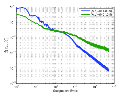
Figure 1: Problem (65): Log of square distance to the (unique) solution vs log of number of subgradient evaluations for two decaying stepsizes.

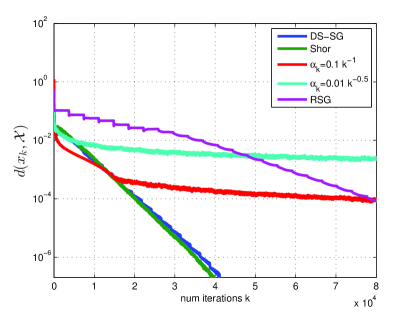
Figure 2: Problem (65): Log of square distance to the (unique) solution vs number of subgradient evaluations for DS-SG, RSG, and two decaying stepsizes.

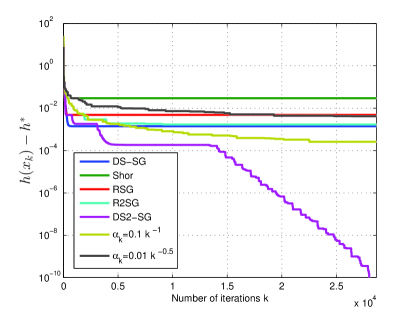
Figure 3: Problem (65): Log of $h(x)-h^{*}$ vs number of subgradient evaluations for DS-SG, RSG, and Shor’s method all with $c=100$, R²SG, DS2-SG with the initial $c_{1}=G=160$, and two decaying stepsizes.

As was mentioned we had to tune $c$ to get good performance of DS-SG, RSG, and Shor’s method. We now compare these three methods with our proposed ’doubling trick’ variant DS2-SG, which does not need the value of $c$. We also compare with the method R²SG proposed in yang2015rsg . Note that this method only works for $\theta<1$ so following the advice of yang2015rsg , we use the approximate value of $\hat{\theta}=0.8$, which was chosen because it performed well. We initialize DS2-SG with the same parameters as DS-SG but with $c_{1}=G=160$. To demonstrate the effect of poorly chosen $c$ in DS-SG, RSG, and Shor’s method, we set $c=100$ for all these methods (recall the tuned values were smaller). The results are given in Fig. 3. We compare function values and for each algorithm we keep track of the iterate with the smallest function value so far. We see that DS-SG, RSG, and Shor’s method converge to suboptimal solutions due to the incorrect value of $c$. However DS2-SG finds the correct solution to within an objective function error of $10^{-10}$. R²SG has slower convergence, which is not surprising since it is not guaranteed to obtain linear convergence when $\theta=1$. It is also encouraging that DS2-SG is faster than the decaying stepsizes $\alpha_{k}=O(k^{-1})$ and $\alpha_{k}=O(k^{-0.5})$, since this choice also does not require knowledge of $c$.

10.2 Least-Absolute Deviations Regression on the “space.ga” Dataset

We also apply Prob. (65) on a real dataset. We use the normalized space.ga dataset downloaded from the libsvm website. We use a subset of the dataset with $m=100$ and $n=6$, and set $\tau=5$.

Since $c$ is unknown, we compare subgradient methods which do not require it. Thus we compare two decaying stepsizes, $\alpha_{k}=k^{-1}$ and $\alpha_{k}=0.1k^{-0.5}$, and DS2-SG. Note that R²SG also does not require $c$ but we could not tune it to be competitive on this problem. For DS2-SG, we estimate $G=\sum_{i=1}^{n}\|E_{i}\|$ and $\Omega_{{\mathcal{C}}}=4\tau^{2}$ as in the synthetic experiment. We use $\beta_{ds}=2$ and $\epsilon=10^{-12}$. The objective function vs iteration-number is plotted in Fig. 4. One can see that the decaying stepsizes are faster than DS2-SG in the early iterations but DS2-SG is much faster in the later iterations. The decaying stepsizes were highly sensitive to the choice of $\alpha_{1}$ which had to be tuned. On the other hand DS-SG was effected by the choice of $\beta_{ds}$. Smaller values of $\beta_{ds}$ lead to better performance early-on, while larger values give better convergence in the latter iterations. In general $\beta_{ds}\in[1.5,4]$ worked well in all of our experiments.

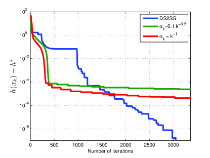
Figure 4: Problem (65) applied to space.ga dataset: Log of $h(x)-h^{*}$ vs number of subgradient evaluations for DS-SG, $\alpha_{k}=k^{-1}$, and $\alpha_{k}=0.1k^{-0.5}$.

10.3 Sparse SVM

The $\ell_{1}$-regularized Support Vector Machine (SVM) Problem zhu20031 is

$$\min_{x\in\mathbb{R}^{n}}\sum_{i=1}^{m}\max\{0,1-y_{i}c_{i}^{\top}x\}+\rho\|x\|_{1}$$

for a dataset $\{c_{i},y_{i}\}_{i=1}^{m}$ with $c_{i}\in\mathbb{R}^{n}$ and $y_{i}\in\{\pm 1\}$. We will consider the equivalent constrained version

$$\min_{x\in\mathbb{R}^{n}}\sum_{i=1}^{m}\max\{0,1-y_{i}c_{i}^{\top}x\}:\|x\|_{1}\leq\tau.$$ (66)

Since the objective function is polyhedral it satisfies HEB with $\theta=1$ for some unknown $c>0$. Once again since $c$ is unknown, we only consider DS2-SG, R²SG yang2015rsg , and the following decaying stepsizes: $\alpha_{k}=0.1k^{-1}$ and $\alpha_{k}=0.01k^{-0.5}$, where the constants $0.1$ and $0.01$ were tuned to give fast convergence. R²SG only works for $\theta<1$ so cannot be directly applied to this problem. Instead we selected $\hat{\theta}<1$ which gave the fastest convergence. Surprisingly, $\hat{\theta}=0.5$ performed the best even though one might expect $\hat{\theta}\approx 1$ to perform better. For DS2-SG we initialize with $c_{1}=G$ where $G=\sum_{i=1}^{m}\|c_{i}\|$. We used $\beta_{ds}=2$, $\epsilon=10^{-5}$, and $\Omega_{{\mathcal{C}}}=4\tau^{2}$. All four algorithms had the same starting point.

A random instance of Prob. (66) was generated as follows: $n=50$, $m=100$, the entries of $c_{i}$ are drawn from $\mathcal{N}(0,1)$, the $y_{i}=\pm 1$ with equal probability, and $\tau=2$. The results are plotted in Fig. 5. We see that our proposal, DS2-SG, outperforms the others.

10.4 Sparse SVM on the “glass.scale” Dataset

To test Prob. (66) on real data, we download the glass.scale dataset from the libsvm website. For this dataset, $n=9$ and $m=214$. There are $6$ different labels so we group labels “1”, “2”, and “3” together into class: $y=-1$, and labels “5”, “6”, and “7” into class: $y=1$. We solve Prob. (66) with $\tau=2$.

Again we compare the subgradient methods which do not require $c$, namely DS2-SG, R²SG, and two decaying stepsizes. For DS2-SG we use the same parameters as in the synthetic experiment, except $\beta_{ds}=4$ and $\epsilon=10^{-8}$. The objective function vs iteration-number is plotted in Figure 6. Once again we see that DS2-SG outperforms the two decaying stepsizes as well as R²SG.

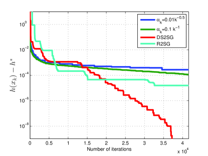
Figure 5: Problem (66) with randomly generated data: Log of $h(x)-h^{*}$ vs number of subgradient evaluations for DS2-SG, R²SG, and two decaying stepsizes.

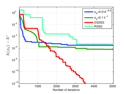
Figure 6: Problem (66) for the “glass.scale” dataset: Log of $h(x)-h^{*}$ vs number of subgradient evaluations for DS2-SG, R²SG, and two decaying stepsizes.

11 Extensions

As previously mentioned, the key recursion (4) can also be derived in the following situations: 1) when a small amount of noise is added to the subgradient, 2) for the incremental subgradient method, 3) under a more general condition than HEB, introduced by Goffin goffin1977convergence , 4) for the proximal subgradient method, and 5) for relaxed versions of the subgradient method. We now discuss the first three of these in more detail.

11.1 Deterministic Noise in the Subgradient when $\theta=1$

For the weakly sharp case ($\theta=1$), the subgradient method exhibits resilience to bounded noise. This has been observed in nedic2010effect ; poljak1978nonlinear . Suppose that at each iteration we have access to a noisy subgradient:

$$\tilde{g}_{k}=g_{k}+r_{k}:g_{k}\in\partial h(x_{k}),\|r_{k}\|\leq R$$

and as before the method iterates for all $k\geq 0$

$$x_{k+1}=P_{{\mathcal{C}}}(x_{k}-\alpha_{k}\tilde{g}_{k}).$$

One can repeat the analysis of Sec. 3.2 to show

$$d(x_{k+1},{\mathcal{X}}_{h})^{2} \leq d(x_{k},{\mathcal{X}}_{h})^{2}-2\alpha_{k}d(x_{k},{\mathcal{X}}_{h})(c-R)+2\alpha_{k}^{2}(R^{2}+G^{2}).$$

We see that this is exactly the same recursion as (5) with the error bound constant $c$ replaced by $c-R$, and $G^{2}$ replaced by $2(G^{2}+R^{2})$. Thus, if $R<c$, all of the results presented throughout for $\theta=1$ hold with a new error bound constant $\tilde{c}=c-R$, and bound on the subgradients $\tilde{G}^{2}=2(G^{2}+R^{2})$. In particular this refers to Theorems 4.1, 5.1, 6.1, 7.1, and 9.2.

11.2 Incremental Subgradient Methods

Suppose $h(x)=\sum_{i=1}^{m}h_{i}(x)$. Such objective functions which are a finite sum of terms often arise in machine learning in the guise of empirical risk minimization hastie2009elements . For such problems the incremental subgradient method can be used nedic2001convergence . This method proceeds by computing the subgradient with respect to each individual function $h_{i}$ in a fixed order. More precisely the method proceeds for $k\geq 1$ with $x_{1}\in{\mathcal{C}}$ as

$$x_{k+1} = \psi_{m,k}$$ (67)

$$\psi_{i,k} = P_{\mathcal{C}}(\psi_{i-1,k}-\alpha_{k}g_{i,k}),g_{i,k}\in\partial h_{i}(\psi_{i-1,k}),\,\,\,i=1,\ldots,m$$ (68)

$$\psi_{0,k} = x_{k}.$$ (69)

This method has been analyzed extensively in nedic2001convergence .

Proposition 3 (nedic2001convergence )

Suppose Assumption 3 holds. Then for all $k\geq 1$ the iterates of (67)–(69) satisfy

$$d(x_{k+1},{\mathcal{X}})^{2}\leq d(x_{k},{\mathcal{X}})^{2}-2\alpha_{k}cd(x_{k},{\mathcal{X}})^{\frac{1}{\theta}}+\alpha_{k}^{2}m^{2}G^{2}.$$

This is the same as the main recursion we analyze in (5) with $G^{2}$ replaced by $m^{2}G^{2}$. Thus all our results in the following sections apply to the incremental subgradient method (67)–(69) with this change in constants.

11.3 Goffin’s Condition Number

Goffin goffin1977convergence discussed a condition number for quantifying the convergence rate of subgradient methods. The condition number is a generalization of the ordinary notion defined for a smooth strongly convex function as the ratio of the Lipschitz constant of the gradient to the strong convexity parameter. In contrast Goffin’s condition number requires neither smoothness or strong convexity. The condition number is also more general than Shor’s eccentricity measure shor2012minimization . The condition number for a convex function $h$ is defined as

$$\mu_{h}=\inf\left\{\frac{\langle u,x-x^{*}_{p}\rangle}{\|u\|\|x-x_{p}^{*}\|}:x\in{\mathcal{C}}\backslash{\mathcal{X}}_{h},u\in\partial h(x),x_{p}^{*}=\text{proj}_{{\mathcal{X}}_{h}}(x)\right\}.$$ (70)

By convexity and the Cauchy-Schwarz inequality $0\leq\mu_{h}\leq 1$. Goffin showed that if $h$ satisfies HEB$(c,\theta)$ with $\theta=1$ and $\|g\|\leq G$ for all $g\in\partial h(x),x\in{\mathcal{C}}$, then it satisfies (70) with

$$\mu_{h}\geq\frac{c}{G}=\frac{1}{\kappa}$$

which proves that functions satisfying (70) with $\mu_{h}>0$ are more general than weakly sharp functions.

Our results for $\theta=1$ throughout this manuscript can be extended to functions satisfying (70) with $\mu_{h}>0$ if we make a slight modification to the subgradient method.

Lemma 1 (goffin1977convergence )

Let $\{x_{k}\}$ be a sequence satisfying

$$x_{k+1}=P_{\mathcal{C}}\left(x_{k}-\alpha_{k}\frac{g_{k}}{\|g_{k}\|}\right):\forall k\geq 1,g_{k}\in\partial h(x_{k}),x_{1}\in{\mathcal{C}}.$$ (71)

If ${\mathcal{X}}_{h}$ is nonempty and $h$ is convex, closed, and proper (CCP) and satisfies (70) with $\mu_{h}>0$, then for all $k\geq 1$

$$d(x_{k+1},{\mathcal{X}}_{h})^{2}\leq d(x_{k},{\mathcal{X}}_{h})^{2}-2\alpha_{k}\mu_{h}d(x_{k},{\mathcal{X}}_{h})+\alpha_{k}^{2}.$$

This is the same recursion as (5) with $G=1$, $\theta=1$, and $c=\mu_{h}$. Thus all the results derived in this manuscript for HEB with $\theta=1$ can be derived for the scheme (71) applied to functions satisfying (70) so long as $c$ is replaced by $\mu_{h}$ and $G=1$. Also note that Lemma 1 does not require that the subgradients are uniformly bounded over ${\mathcal{C}}$.

12 Proof of Theorems 9.1, 9.2, and 9.3

12.1 Preliminaries

In order to determine the convergence rate of the recursion (5) derived in Prop. 1 under generic nonsummable stepsizes, we need two Lemmas. We start with a result from PolyakIntro which considers (5) when $\theta<\frac{1}{2}$ without the nuisance term $\alpha_{k}^{2}G^{2}$.

Lemma 2

Suppose

$$0\leq u_{k+1}\leq u_{k}-\gamma_{k}u_{k}^{1+q}$$

for $k=0,1,\ldots$ where $\gamma_{k}\geq 0$ and $q>0$. Then

$$u_{k}\leq u_{0}\left(1+qu_{0}^{q}\sum_{i=0}^{k-1}\gamma_{i}\right)^{-\frac{1}{q}}.$$

Proof

(PolyakIntro, , Lemma 6 pp. 46).

We will also use the following estimates for the sum of stepsizes $\sum_{i=k_{0}}^{k}\alpha_{i}$.

Lemma 3

Let $k\geq k_{0}\geq 1$.

1. If $p\in(0,1)$

   $$\sum_{i=k_{0}}^{k}i^{-p}\geq\frac{(k+1)^{1-p}-k_{0}^{1-p}}{1-p}.$$

2. If $p=1$

   $$\sum_{i=k_{0}}^{k}i^{-p}\geq\ln\frac{k+1}{k_{0}}.$$

Proof

A straightforward integral test.

12.2 Main Proof for Theorems 9.1 and 9.2

Continuing with the main analysis, the goal is to derive convergence rates for a sequence $e_{k}$ satisfying (5). To this end, let

$$I=\{k:\alpha_{k}G^{2}\geq ce_{k}^{\gamma}\}.$$ (72)

Recall the notation $\gamma=1/(2\theta)$. We will consider three types of iterates and bound the convergence rate in each case. First, for those iterates $k\in I$ it is easy to derive the convergence rate. Second, we will bound the rate for an iterate in $I^{c}$ when the previous iterate is in $I$. Finally we will consider $s$ consecutive iterates in $I^{c}$, for which we can use the inequality in (72) to simplify recursion (5). Note that $s$ can be arbitrarily large. In particular when $I$ is finite there are an unbounded number of consecutive iterates in $I^{c}$. Together these three cases cover all possible iterates.

First for, $k\in I$ and $\alpha_{k}>0$

$$\alpha_{k}ce_{k}^{\gamma}\leq\alpha_{k}^{2}G^{2}\implies e_{k}\leq\left(\frac{\alpha_{k}G^{2}}{c}\right)^{\frac{1}{\gamma}}.$$

Thus the rate of $e_{k}$ is $O\left(\alpha_{k}^{\frac{1}{\gamma}}\right)$ for $k\in I$. In particular since $\alpha_{k}=\alpha_{1}k^{-p}$, then for $k\in I$ and $\alpha_{1}>0$

$$e_{k}\leq\left(\frac{\alpha_{1}G^{2}}{c}\right)^{2\theta}k^{-2p\theta}.$$ (73)

Now assume $k\in I$ and $k+1\in I^{c}$. Then

$$e_{k+1}\leq e_{k}+\alpha_{k}^{2}G^{2}\leq\left(\frac{\alpha_{k}G^{2}}{c}\right)^{\frac{1}{\gamma}}+\alpha_{k}^{2}G^{2}.$$ (74)

Now since $\frac{1}{\gamma}=2\theta\in(0,2)$, for $k\geq 1$

$$k^{-2p\theta}\geq k^{-2p}.$$

Therefore (74) implies that for $k\in I$, $k+1\in I^{c}$, and $k\geq 1$,

$$e_{k+1} \leq C_{1}(k+1)^{-2p\theta}$$ (75)

where

$$C_{1}=2^{2p\theta}\left(\left(\frac{\alpha_{1}G^{2}}{c}\right)^{\frac{1}{\gamma}}+\alpha_{1}^{2}G^{2}\right).$$

Next assume $k\in I$, $k+1\in I^{c}$, and $k+i\in I^{c}$ for $i=2,\ldots s$ for some $s\geq 2$. Then for $i=2,\ldots s$

$$e_{k+i}<e_{k+i-1}-\alpha_{k}ce_{k+i-1}^{\gamma}.$$ (76)

To analyze the recursion (76) we consider $\theta<\frac{1}{2}$ and $\theta\geq\frac{1}{2}$ separately.

Case 1: $\boldsymbol{\theta<\frac{1}{2}}$.

Now since $\gamma>1$ we can apply Lemma 2 along with Lemma 3 to (76) and derive for $i=2,\ldots,s$

$$e_{k+i} \leq e_{k+1}\left[1+\frac{1-2\theta}{2\theta}e_{k+1}^{\frac{1-2\theta}{2\theta}}\sum_{j=1}^{i-1}\alpha_{k+j}\right]^{\frac{2\theta}{2\theta-1}}$$

$$\leq e_{k+1}\left[1+\frac{\alpha_{1}(1-2\theta)}{2\theta(1-p)}e_{k+1}^{\frac{1-2\theta}{2\theta}}\left((k+i)^{1-p}-(k+1)^{1-p}\right)\right]^{\frac{2\theta}{2\theta-1}}.$$ (77)

Now consider the condition given in (59). Note that since $p$ satisfies (58), if (59) holds for $k=k_{0}$, it holds for all $k>k_{0}$. In particular if it holds for $k=0$, then it holds for all $k$. Continuing, if (59) holds then for all $k>k_{0}$

$$1-\frac{\alpha_{1}(1-2\theta)}{2\theta(1-p)}e_{k+1}^{\frac{1-2\theta}{2\theta}}(k+1)^{1-p}\geq 0$$ (78)

where we have used the fact that $k+1\in I^{c}$. Therefore since (78) holds we can simplify (77) to say that for $k\in I$ and $k+i\in I^{c}$ for $i=2,3,\ldots,s$, and $k>k_{0}$,

$$e_{k+i} \leq e_{k+1}\left[\frac{\alpha_{1}(1-2\theta)}{2\theta(1-p)}e_{k+1}^{\frac{1-2\theta}{2\theta}}(k+i)^{1-p}\right]^{\frac{2\theta}{2\theta-1}}$$ (79)

$$\leq \left(\frac{\alpha_{1}(1-2\theta)}{2\theta(1-p)}\right)^{\frac{2\theta}{2\theta-1}}(k+i)^{\frac{2\theta(1-p)}{2\theta-1}}.$$

The final case to consider is when $i=1,2,\ldots,s$ are in $I^{c}$. In this case, the same bound (77) can be derived but with $e_{1}$ replacing $e_{k+1}$. Thus for $i=2,3,\ldots s$ in $I$

$$e_{i}\leq e_{1}\left[1+\frac{\alpha_{1}(1-2\theta)}{2\theta(1-p)}e_{1}^{\frac{1-2\theta}{2\theta}}\left(i^{1-p}-1\right)\right]^{\frac{2\theta}{2\theta-1}}.$$ (80)

Thus if $\alpha_{1}$ is chosen to satisfy (60) then

$$e_{i}\leq\left(\frac{\alpha_{1}(1-2\theta)}{2\theta(1-p)}\right)^{\frac{2\theta}{2\theta-1}}i^{\frac{2\theta(1-p)}{2\theta-1}}.$$ (81)

Combining (73), (75), (79), and (81) establishes (61) and concludes the proof of Theorem 9.1.

Case 2: $\boldsymbol{\theta\geq\frac{1}{2}}$

Next we consider the case where $\frac{1}{2}\leq\theta\leq 1$ which will finish the proof of Theorem 9.2. Before commencing we introduce the following Lemma which allows us to bound a decaying exponential by an appropriately scaled decaying polynomial of any degree.

Lemma 4

Suppose $\delta>0$, then if $C_{\delta}\geq e^{-\delta}\delta^{\delta}$,

$$\exp(-x)\leq C_{\delta}x^{-\delta}\quad\forall x>0.$$ (82)

Proof

Taking logs of both sides of (82) yields

$$-x\leq-\delta\ln x+\beta_{\delta}\quad\forall x>0$$

where $\beta_{\delta}=\ln C_{\delta}$. Therefore

$$\beta_{\delta} \geq \delta\ln x-x\quad\forall x>0$$

which implies

$$\beta_{\delta} \geq \max_{x>0}\{\delta\ln x-x\}.$$

The right hand side is a smooth concave coercive maximization problem which therefore has a unique solution given by $x^{*}=\delta$. Hence

$$\beta_{\delta}\geq\delta\ln\delta-\delta$$

which implies the Lemma.

Continuing, we consider $k\in I$, $k+1\in I^{c}$, and $k+i\in I^{c}$ for $i=2\ldots,s$ in the case where $\theta\geq\frac{1}{2}$, so $\gamma\leq 1$. Then since $k+i\in I^{c}$ for $i=2,\ldots s$,

$$0\leq\frac{e_{k+i-1}}{e_{k+1}}\leq 1\implies\left(\frac{e_{k+i-1}}{e_{k+1}}\right)^{\gamma}\geq\frac{e_{k+i-1}}{e_{k+1}}\implies e_{k+i-1}^{\gamma}\geq e_{k+1}^{\gamma-1}e_{k+i-1}.$$

Thus for $k\in I$, $k+1\in I^{c}$, and $k+i\in I^{c}$ for $i=2,\ldots,s$ for some $s\geq 2$

$$e_{k+i} \leq e_{k+i-1}-\alpha_{k+i-1}ce_{k+i-1}^{\gamma}$$

$$\leq e_{k+i-1}-\alpha_{k+i-1}e_{k+1}^{\gamma-1}ce_{k+i-1}.$$ (83)

Now taking logs and using $\log(1-x)\leq-x$,

$$\ln e_{k+i} \leq \ln e_{k+i-1}+\ln(1-e_{k+1}^{\gamma-1}c\alpha_{k+i-1})$$

$$\leq \ln e_{k+i-1}-e_{k+1}^{\gamma-1}c\alpha_{k+i-1}.$$

Now summing and using Lemma 3

$$\ln e_{k+i} \leq \ln e_{k+1}-\alpha_{1}e_{k+1}^{\gamma-1}c\sum_{i=k+1}^{k+i-1}i^{-p}$$

$$\leq \ln e_{k+1}-\frac{\alpha_{1}e_{k+1}^{\gamma-1}c}{1-p}\left((k+i)^{1-p}-(k+1)^{1-p}\right).$$

This leads to

$$e_{k+i} \leq e_{k+1}\exp\left\{-\frac{\alpha_{1}e_{k+1}^{\gamma-1}c}{1-p}\left((k+i)^{1-p}-(k+1)^{1-p}\right)\right\}$$

$$= \exp\left\{-\frac{\alpha_{1}e_{k+1}^{\gamma-1}c(k+i)^{1-p}}{1-p}\left(1-\left(\frac{k+1}{k+i}\right)^{1-p}\right)\right\}.$$

We further consider two possible cases. If $i\geq k$, then

$$\frac{k+1}{k+i}\leq\frac{k+1}{k+k}=\frac{1}{2}+\frac{1}{2k}$$

therefore by concavity of $t^{1-p}$

$$\left(\frac{k+1}{k+i}\right)^{1-p}\leq 2^{p-1}\left[1+\frac{1-p}{k}\right].$$

Take $k>3$ so that

$$\frac{2^{p-1}(1-p)}{k}\leq\frac{1-2^{p-1}}{2}.$$

Hence

$$1-\left(\frac{k+1}{k+i}\right)^{1-p}\geq 1-2^{p-1}\left[1+\frac{1-p}{k}\right]\geq 1-2^{p-1}-\frac{2^{p-1}(1-p)}{k}\geq\frac{1-2^{p-1}}{2}.$$

Hence if $3<k\leq i$ then

$$e_{k+i} \leq e_{k+1}\exp\left(-\frac{(1-2^{p-1})\alpha_{1}e_{k+1}^{\gamma-1}c}{2(1-p)}(k+i)^{1-p}\right).$$ (85)

Now by Lemma 4 for any $\delta_{1}>0$,

$$\exp\left\{-\frac{\alpha_{1}(1-2^{p-1})ce_{k+1}^{\gamma-1}}{2(1-p)}(k+i)^{1-p}\right\}$$

$$\leq \delta_{1}^{\delta_{1}}e^{-\delta_{1}}e_{k+1}^{1+\delta_{1}(1-\gamma)}\left(\frac{\alpha_{1}(1-2^{p-1})c}{2(1-p)}(k+i)^{1-p}\right)^{-\delta_{1}}.$$

Therefore using (75) for any $k\leq i$ and $k>3$

$$e_{k+i} \leq \delta_{1}^{\delta_{1}}C_{1}^{1+\delta_{1}(1-\gamma)}\left(\frac{\alpha_{1}(1-2^{p-1})ce}{2(1-p)}\right)^{-\delta_{1}}(k+i)^{-\delta_{1}(1-p)}.$$ (86)

Taking $\delta_{1}=\frac{2p\theta}{1-p}$ and simplifying (86) yields

$$e_{k+i} \leq C_{1}^{\frac{1+2p(\theta-1)}{1-p}}\left(\frac{\alpha_{1}(1-2^{p-1})ce}{4p\theta}\right)^{-\frac{2p\theta}{1-p}}(k+i)^{-2p\theta}.$$ (87)

Next consider $k\geq i>1$. Now

$$(k+i)^{1-p}-(k+1)^{1-p} = (k+i)^{1-p}\left(1-\left(\frac{k+1}{k+i}\right)^{1-p}\right)$$

$$= (k+i)^{1-p}\left(1-\left(1-\frac{i-1}{k+i}\right)^{1-p}\right)$$

$$\geq (k+i)^{1-p}\left(1-\left(1-\frac{i-1}{2k}\right)^{1-p}\right)$$

$$\geq \frac{(1-p)(k+i)^{1-p}(i-1)}{2k}$$

$$\geq \frac{1-p}{2}k^{-p}(i-1)$$

where in (12.2) we used the concavity of $t^{1-p}$. Thus substituting this into (12.2) implies for $k\geq i$

$$e_{k+i}\leq e_{k+1}\exp\left(\frac{-\alpha_{1}e_{k+1}^{\gamma-1}c(i-1)}{2k^{p}}\right).$$

Therefore for all $\delta_{2}\geq 0$ it follows Lemma 4 that

$$e_{k+i} \leq e_{k+1}\exp\left(\frac{-\alpha_{1}e_{k+1}^{\gamma-1}c(i-1)}{2k^{p}}\right)$$ (89)

$$\leq \delta_{2}^{\delta_{2}}e_{k+1}\left(\frac{\alpha_{1}e_{k+1}^{\gamma-1}c(i-1)e}{2k^{p}}\right)^{-\delta_{2}}$$

$$\leq C_{1}^{1+\delta_{2}(1-\gamma)}\left(\frac{4\delta_{2}}{c\alpha_{1}e}\right)^{\delta_{2}}k^{-2p\theta(1+\delta_{2}(1-\gamma))}k^{p\delta_{2}}i^{-\delta_{2}}$$

where we used $e_{k+1}\leq C_{1}k^{-2p\theta}$ and $(i-1)^{-\delta_{2}}\leq 2^{\delta_{2}}i^{-\delta_{2}}$. Now if we choose

$$\delta_{2}=2\theta$$ (90)

then (89) implies

$$e_{k+i}\leq C_{4}i^{-2\theta}$$ (91)

where

$$C_{4}=\left(\frac{8\theta C_{1}}{c\alpha_{1}e}\right)^{2\theta}.$$ (92)

Thus combining $e_{k+i}\leq e_{k+1}\leq C_{1}k^{-2p\theta}$ and (91) implies that for $i\leq k$

$$e_{k+i}\leq\max\{C_{1},C_{4}\}\min\{k^{-2p\theta},i^{-2\theta}\}.$$

Now since $-2\theta<-2p\theta$,

$$e_{k+i}\leq\max\{C_{1},C_{4}\}\min\{k^{-2p\theta},i^{-2p\theta}\}\leq\frac{\max\{C_{1},C_{4}\}}{\max\{k^{2p\theta},i^{2p\theta}\}}.$$

If $2p\theta\geq 1$ then by convexity of $t^{2p\theta}$

$$\max\{k^{2p\theta},i^{2p\theta}\}\geq\frac{1}{2}\left(k^{2p\theta}+i^{2p\theta}\right)\geq 2^{-2p\theta}\left(k+i\right)^{2p\theta}.$$ (93)

On the other hand if $2p\theta<1$ then because $t^{2p\theta}$ is subadditive

$$\max\{k^{2p\theta},i^{2p\theta}\}\geq\frac{1}{2}\left(k^{2p\theta}+i^{2p\theta}\right)\geq\frac{1}{2}\left(k+i\right)^{2p\theta}.$$ (94)

Combining (93) and (94) gives

$$e_{k+i}\leq 4\max\{C_{1},C_{4}\}(k+i)^{-2p\theta}.$$ (95)

Finally we consider the case where the first $s$ iterates belong to $I^{c}$. Therefore, using (12.2), for $i=1,2,\ldots,s$

$$e_{i} \leq e_{1}\exp\left\{-\frac{\alpha_{1}e_{1}^{\gamma-1}c}{1-p}\left(i^{1-p}-1\right)\right\}.$$ (96)

Now since for $x\geq 1$, $x-1\geq\frac{x}{2}$, this implies that

$$e_{i} \leq e_{1}\exp\left\{-\frac{\alpha_{1}e_{1}^{\gamma-1}c}{2(1-p)}i^{1-p}\right\}.$$

Using Lemma 4 this implies that for any $\delta_{3}>0$

$$e_{i} \leq e^{-\delta_{3}}\delta_{3}^{\delta_{3}}e_{1}\left(\frac{\alpha_{1}e_{1}^{\gamma-1}c}{2(1-p)}i^{1-p}\right)^{-\delta_{3}}.$$ (97)

and we will use $\delta_{3}=\frac{2p\theta}{1-p}$.

Combining (73), (75), (87), (95), and (97) yields the desired result (63) and concludes the proof of Theorem 9.2.

12.3 Proof of Theorem 9.3

The format of the proof is identical to Theorems 9.1 and 9.2. As before it is based on the set $I$ defined in (72) and we consider three types of iterates. First we bound the convergence rate for iterates in $I$, second for iterates in $I^{c}$ when the previous iterate is in $I$. And finally for $s$ consecutive iterates in $I^{c}$ where $s$ may be unbounded.

If $k\in I$ then repeating (75) yields

$$e_{k}\leq\frac{\alpha_{1}G^{2}}{c}k^{-1}.$$ (98)

Similarly for $k\in I$ and $k+1\in I^{c}$,

$$e_{k+1}\leq\frac{2\alpha_{1}G^{2}}{c}(k+1)^{-1}.$$ (99)

Finally for $k\in I$, $k+1\in I^{c}$, and $k+i\in I^{c}$, for $i=2,\ldots,s$, then repeating (83) but with $\gamma=1$ this time,

$$e_{k+i}\leq e_{k+i-1}(1-c\alpha_{k+i-1}).$$

Taking logs, using $\log(1-x)\leq-x$ and summing yields

$$\log e_{k+i} \leq \log e_{k+1}-c\alpha_{1}\sum_{j=k+1}^{k+i-1}j^{-1}$$

$$\leq \log e_{k+1}-c\alpha_{1}\left(\log(k+i)-\log(k+1)\right)$$

where we applied Lemma 3 in the second inequality. This yields for all $k\in I$ and $k+i\in I^{c}$ for $i=2,3,\ldots,s$ for some $s\in\mathbb{N}$

$$e_{k+i} \leq e_{k+1}\left(\frac{k+i}{k+1}\right)^{-c\alpha_{1}}.$$ (100)

Using (99) yields

$$e_{k+i} \leq \frac{2\alpha_{1}G^{2}}{c}(k+1)^{-1}(k+1)^{c\alpha_{1}}(k+i)^{-c\alpha_{1}}$$ (101)

$$\leq \frac{2\alpha_{1}G^{2}}{c}(k+i)^{-c\alpha_{1}}$$

Finally we consider the case where the initial iterates $i=1,2,\ldots,s$ are in $I^{c}$. Therefore repeating (100) with $k=0$ gives

$$e_{i} \leq e_{1}i^{-c\alpha_{1}}$$ (102)

Combining (98), (99), (101), and (102) yields (64) and concludes the proof of Theorem 9.3.

12.4 Proof of Proposition 2

As previously mentioned, this argument is a direct extension of (karimi2016linear, , Thm. 4). For $\theta=\frac{1}{2}$, (5) reads as

$$e_{k+1}\leq(1-2\alpha_{k}c)e_{k}+\alpha_{k}^{2}G^{2}.$$

We consider the choice $\alpha_{k}=\frac{2k+1}{2c(k+1)^{2}}$. Then

$$e_{k+1}\leq\left(1-\frac{2k+1}{(k+1)^{2}}\right)e_{k}+\frac{G^{2}(2k+1)^{2}}{4c^{2}(k+1)^{4}}.$$

Multiplying both sides by $(k+1)^{2}$ yields

$$(k+1)^{2}e_{k+1} \leq k^{2}e_{k}+\frac{G^{2}(2k+1)^{2}}{4c^{2}(k+1)^{2}}$$

$$\leq k^{2}e_{k}+\frac{G^{2}}{c^{2}}$$

$$\leq e_{1}+\frac{G^{2}}{c^{2}}k.$$

Therefore

$$e_{k+1}\leq\frac{e_{1}}{(k+1)^{2}}+\frac{G^{2}}{c^{2}(k+1)}.$$

Acknowledgments. We thank Prof. Niao He for many illuminating and important discussions.

References

- (1) Agrb, G.: Maximum likelihood and -—norm estimators. Statistics Applicata 4(1), 7 (1992)
- (2) Attouch, H., Bolte, J., Svaiter, B.F.: Convergence of descent methods for semi-algebraic and tame problems: proximal algorithms, forward–backward splitting, and regularized Gauss–Seidel methods. Mathematical Programming 137(1-2), 91–129 (2013)
- (3) Barrodale, I., Roberts, F.D.: An improved algorithm for discrete linear approximation. SIAM Journal on Numerical Analysis 10(5), 839–848 (1973)
- (4) Bauschke, H.H., Combettes, P.L.: Convex Analysis and Monotone Operator Theory in Hilbert Spaces. Springer Science & Business Media (2011)
- (5) Beck, A., Shtern, S.: Linearly convergent away-step conditional gradient for non-strongly convex functions. Mathematical Programming pp. 1–27 (2015)
- (6) Bertsekas, D.P.: Nonlinear Programming, 2nd edn. Athena Scientific (1999)
- (7) Bolte, J., Daniilidis, A., Lewis, A.: The Łojasiewicz inequality for nonsmooth subanalytic functions with applications to subgradient dynamical systems. SIAM Journal on Optimization 17(4), 1205–1223 (2007)
- (8) Bolte, J., Nguyen, T.P., Peypouquet, J., Suter, B.W.: From error bounds to the complexity of first-order descent methods for convex functions. Mathematical Programming pp. 1–37 (2015)
- (9) Bubeck, S., et al.: Convex optimization: Algorithms and complexity. Foundations and Trends® in Machine Learning 8(3-4), 231–357 (2015)
- (10) Burke, J., Deng, S.: Weak sharp minima revisited part i: basic theory. Control and Cybernetics 31, 439–469 (2002)
- (11) Burke, J., Ferris, M.C.: Weak sharp minima in mathematical programming. SIAM Journal on Control and Optimization 31(5), 1340–1359 (1993)
- (12) Chambolle, A., Pock, T.: A first-order primal-dual algorithm for convex problems with applications to imaging. Journal of Mathematical Imaging and Vision 40(1), 120–145 (2011)
- (13) Cruz, J.Y.B.: On proximal subgradient splitting method for minimizing the sum of two nonsmooth convex functions. Set-Valued and Variational Analysis 25(2), 245–263 (2017)
- (14) Davis, D., Yin, W.: A three-operator splitting scheme and its optimization applications. Set-valued and variational analysis 25(4), 829–858 (2017)
- (15) Duchi, J., Shalev-Shwartz, S., Singer, Y., Chandra, T.: Efficient projections onto the -ball for learning in high dimensions. In: Proceedings of the 25th International Conference on Machine Learning, pp. 272–279. ACM (2008)
- (16) Eckstein, J., Yao, W.: Augmented Lagrangian and alternating direction methods for convex optimization: A tutorial and some illustrative computational results. RUTCOR Research Reports 32 (2012)
- (17) Efron, B., Hastie, T., Johnstone, I., Tibshirani, R., et al.: Least angle regression. The Annals of Statistics 32(2), 407–499 (2004)
- (18) Ferris, M.C.: Finite termination of the proximal point algorithm. Mathematical Programming 50(1), 359–366 (1991)
- (19) Freund, R.M., Lu, H.: New computational guarantees for solving convex optimization problems with first order methods, via a function growth condition measure. Mathematical Programming pp. 1–33 (2015)
- (20) Gao, X., Huang, J.: Asymptotic analysis of high-dimensional LAD regression with LASSO. Statistica Sinica pp. 1485–1506 (2010)
- (21) Gilpin, A., Pena, J., Sandholm, T.: First-order algorithm with convergence for -equilibrium in two-person zero-sum games. Mathematical Programming 133(1-2), 279–298 (2012)
- (22) Goffin, J.L.: On convergence rates of subgradient optimization methods. Mathematical Programming 13(1), 329–347 (1977)
- (23) Hare, W., Lewis, A.S.: Identifying active constraints via partial smoothness and prox-regularity. Journal of Convex Analysis 11(2), 251–266 (2004)
- (24) Hastie, T., Tibshirani, R., Friedman, J., Hastie, T., Friedman, J., Tibshirani, R.: The Elements of Statistical Learning. Springer (2009)
- (25) Johnstone, P.R., Moulin, P.: Faster subgradient methods for functions with Hölderian growth. arXiv preprint arXiv:1704.00196 (2017)
- (26) Karimi, H., Nutini, J., Schmidt, M.: Linear Convergence of Gradient and Proximal-Gradient Methods Under the Polyak-Łojasiewicz Condition. In: Joint European Conference on Machine Learning and Knowledge Discovery in Databases, pp. 795–811. Springer (2016)
- (27) Kivinen, J., Smola, A.J., Williamson, R.C.: Online learning with kernels. IEEE Transactions on Signal Processing 52(8), 2165–2176 (2004)
- (28) Li, G.: Global error bounds for piecewise convex polynomials. Mathematical Programming 137(1-2), 37–64 (2013)
- (29) Li, Y., Arce, G.R.: A maximum likelihood approach to least absolute deviation regression. EURASIP Journal on Advances in Signal Processing 2004(12), 948,982 (2004)
- (30) Liang, J., Fadili, J., Peyré, G.: Activity identification and local linear convergence of forward–backward-type methods. SIAM Journal on Optimization 27(1), 408–437 (2017)
- (31) Lim, E.: On the convergence rate for stochastic approximation in the nonsmooth setting. Mathematics of Operations Research 36(3), 527–537 (2011)
- (32) Luo, Z.Q., Tseng, P.: Error bounds and convergence analysis of feasible descent methods: a general approach. Annals of Operations Research 46(1), 157–178 (1993)
- (33) Nedić, A., Bertsekas, D.: Convergence rate of incremental subgradient algorithms. In: Stochastic Optimization: Algorithms and Applications, pp. 223–264. Springer (2001)
- (34) Nedić, A., Bertsekas, D.P.: The effect of deterministic noise in subgradient methods. Mathematical Programming 125(1), 75–99 (2010)
- (35) Nedic, A., Lee, S.: On stochastic subgradient mirror-descent algorithm with weighted averaging. SIAM Journal on Optimization 24(1), 84–107 (2014)
- (36) Nemirovski, A., Juditsky, A., Lan, G., Shapiro, A.: Robust stochastic approximation approach to stochastic programming. SIAM Journal on Optimization 19(4), 1574–1609 (2009)
- (37) Noll, D.: Convergence of non-smooth descent methods using the Kurdyka–Łojasiewicz inequality. Journal of Optimization Theory and Applications 160(2), 553–572 (2014)
- (38) Pang, J.S.: Error bounds in mathematical programming. Mathematical Programming 79(1-3), 299–332 (1997)
- (39) Poljak, B.: Nonlinear programming methods in the presence of noise. Mathematical Programming 14(1), 87–97 (1978)
- (40) Polyak, B.T.: Introduction to Optimization. Optimization Software Inc. (1987)
- (41) Renegar, J.: A framework for applying subgradient methods to conic optimization problems. arXiv preprint arXiv:1503.02611 (2015)
- (42) Renegar, J.: “efficient” subgradient methods for general convex optimization. SIAM Journal on Optimization 26(4), 2649–2676 (2016)
- (43) Rosenberg, E.: A geometrically convergent subgradient optimization method for nonlinearly constrained convex programs. Mathematics of Operations Research 13(3), 512–523 (1988)
- (44) Shor, N.Z.: Minimization Methods for Non-Differentiable Functions, vol. 3. Springer Science & Business Media (2012)
- (45) Supittayapornpong, S., Neely, M.J.: Staggered time average algorithm for stochastic non-smooth optimization with convergence. arXiv preprint arXiv:1607.02842 (2016)
- (46) Tseng, P.: Approximation accuracy, gradient methods, and error bound for structured convex optimization. Mathematical Programming 125(2), 263–295 (2010)
- (47) Wang, L.: The penalized LAD estimator for high dimensional linear regression. Journal of Multivariate Analysis 120, 135–151 (2013)
- (48) Wang, L., Gordon, M.D., Zhu, J.: Regularized least absolute deviations regression and an efficient algorithm for parameter tuning. In: Data Mining, 2006. ICDM’06. Sixth International Conference on, pp. 690–700. IEEE (2006)
- (49) Wu, T.T., Lange, K.: Coordinate descent algorithms for lasso penalized regression. The Annals of Applied Statistics pp. 224–244 (2008)
- (50) Xu, Y., Lin, Q., Yang, T.: Accelerate stochastic subgradient method by leveraging local error bound. arXiv preprint arXiv:1607.01027 (2016)
- (51) Yang, T., Lin, Q.: RSG: beating subgradient method without smoothness and strong convexity. arXiv preprint arXiv:1512.03107 (2015)
- (52) Zhang, H.: New analysis of linear convergence of gradient-type methods via unifying error bound conditions. arXiv preprint arXiv:1606.00269 (2016)
- (53) Zhang, H., Yin, W.: Gradient methods for convex minimization: better rates under weaker conditions. arXiv preprint arXiv:1303.4645 (2013)
- (54) Zhou, Z., So, A.M.C.: A unified approach to error bounds for structured convex optimization problems. Mathematical Programming pp. 1–40 (2017)
- (55) Zhu, J., Rosset, S., Hastie, T., Tibshirani, R.: 1-norm support vector machines. In: NIPS, vol. 15, pp. 49–56 (2003)