Modeling trait-dependent evolution
on a random species tree

Abstract

Understanding the evolution of binary traits, which affects the birth and survival of species and also the rate of molecular evolution, remains challenging. A typical example is the evolution of mating systems in plant species. In this work, we present a probabilistic modeling framework for binary trait, random species trees, in which the number of species and their traits are represented by a two-type, continuous time Markov branching process. We develop our model by considering the impact of mating systems on $dN/dS$, the ratio of nonsynonymous to synonymous substitutions. A methodology is introduced which enables us to match model parameters with parameter estimates from phylogenetic tree data. The properties obtained from the model are applied to outcrossing and selfing species trees in the Geraniaceae and Solanaceae family. This allows us to investigate not only the branching tree rates, but also the mutation rates and the intensity of selection. [mathematical modeling; branching processes; phylogenetic trees; mating systems; $dN/dS$.]

1 Introduction

One of the main obstacles in modern evolutionary biology entails recognizing how different traits evolve on a phylogenetic tree, and how they can affect the evolution of other species characteristics. A popular example is the impact of life history or ecological traits on molecular evolutionary rates ([19]; [23]; [4]). Another subtle hurdle is the difficulty to estimate precisely when a species moved from one character state to another, and how irreversible the change was. These questions have turned out to be particularly difficult to answer; in part, it is simply because what we can observe today, is only what survived, thereby providing a biased view of the evolutionary process. A classical approach involves mapping traits on a phylogenetic tree, and then matching them with the evolutionary rates that have been measured on the corresponding branches. In such approaches, it is usually assumed that the phylogenetic tree is fixed, and is independent of the evolving traits. Yet, it is well known that some traits can affect the diversification process, and hence, the tree shape, which can bias the reconstruction of ancestral states as well as state transitions along the tree [7]. Another strong, and often implicit, assumption is that the change in states only occurs at branching points. In reality, transition may occur along the branches, and this results in diluting the relationship between traits and molecular rates.

A minimal model, addressing the differences in speciation rates between groups, will therefore need to consider, simultaneously, trait evolution and species diversification. The binary-state speciation and extinction (BiSSE) model was precisely developed for this purpose, and it also helped disentangle the two aspects [16]. It was later extended to the ClaSSE (cladogenetic-state speciation and extinction) model. Generally, binary-state phylogenetic models are structured in classes satisfying one or several of [9]:

i) independent speciation and extinction for the two states;

ii) anagenetic change, i.e. instantaneous state change occurring along lineages;

iii) cladogenetic change, i.e. change of state occurring during speciation.

Figure 1 gives an illustration of cladogenetic and anagenetic state changes, in panel a) and panel b), respectively. A BiSSE model satisfies i) and ii), whereas a ClaSSE model shows all properties i), ii) and iii). These models have been extensively used to test for the effect of traits on species diversification. However, to our knowledge, the assessment of the effect of traits on molecular evolutionary rates has neglected to take into account the possible effect of traits on species diversification.

A typical example, where both approaches have been conducted independently, is the evolution of selfing from outcrossing, in the context of the so-called ‘dead-end’ hypothesis [24]. The popular claim that the transition towards selfing is an evolutionary dead-end [13], relies on two hypotheses: the transition from outcrossing to selfing is irreversible, and, selfing species go extinct more often than the outcrossing ones. Both outcrossers and selfers reproduce through the processes of meiosis and fertilization. In the outcrossing species, random fertilization of gametes from distinct individuals occurs, whereas in selfers, gametes from the same hermaphrodite individual fuse together to produce new individuals. In the short term, selfing offers reproductive assurance and transmission advantage over outcrossers, since selfers can contribute to outcross pollen while fertilizing their own ovules at the same time [3]. On the other hand, outcrossing limits a plant’s ability to reproduce in case of rarity of mates. Therefore, the transition from outcrossing to selfing is thought to be one of the most frequent evolutionary changes in angiosperms. In the long run, however, selfing species suffer from negative genetic consequences: selfing reduces effective population sizes and recombination, which globally lessens the efficacy of selection. Selfing species are thus, more prone to the accumulation of deleterious mutations and less able to adapt to changing environments, which eventually drives them towards extinction [27]. In agreement with this prediction and using the BiSSE model, the net diversification rates (difference between speciation and extinction rates) are found to be higher in outcrossing than in selfing Solanaceae species [8]. Generally, it is proposed that the net diversification rate in selfers is negative [13].

In parallel, the negative genetic effects of selfing, which can explain higher extinction rates, were tested by comparing the molecular evolutionary rates between selfing and outcrossing lineages. The efficacy of selection can be assessed through the ratio of nonsynonymous to synonymous substitutions, $dN/dS$; a higher ratio corresponding to less efficient selection. Even though reduced selection efficacy in selfers was often detected at the within-species level, phylogenetic analyses usually failed at detecting any effect of mating system on $dN/dS$ [6]. The recent origin of selfing and the misspecification of shift in mating systems, are generally recognized as the most likely explanations. Yet, the BiSSE or ClaSSE processes underlying the observed trees, have not been incorporated so far, in such $dN/dS$ analyses.

In this work, building on the BiSSE and ClaSSE models, we present a probabilistic modeling framework for binary trait, random species trees, with trait-dependent mutation rates. Similar models have been used in statistical inference, but, to our knowledge, their detailed mathematical properties have not been studied yet. As in the BiSSE and ClaSSE models, the edges of our tree model are grouped into two categories based on a generic trait. Over time, the trait has influenced and shaped the ancestral family tree of the extant species and led eventually to the observable mixture of traits associated with the present tree branches. The model specifies expected values of various random functionals of the tree in terms of basic Markov chain parameters. Not only the number of species of each trait, but also the number of trait-clusters in the tree, as well as the total branch lengths in the ancestral tree, with existing ancestors at the time of observation, are provided.

While the tree model is constructed in forward time, it is the traits and mutations in the ancestral tree seen backwards from the current set of species, that determine the current set of states. In the model, this shift of view corresponds to studying the reduced branching tree, obtained from the original species tree by the removal of extinct species. The rate of fixation, as the species accumulate mutations, may depend on the trait value, due, for example, to a varying degree of selection associated with the traits. Also, considering mutations to be deleterious, the rate of extinction of a species could be a function of the rate of fixation of mutations, in the corresponding trait. The model allows us to study the accumulated number of mutations in relation to the observed distribution of traits.

The analysis helps understand the interplay between the evolution of the trait on one hand, and the mutation activity on the tree branches, on the other. To test our approach with regards to empirical data, we discuss a methodology for matching the model parameters with parameter estimates, using data of reconstructed phylogenetic species trees and draw useful inferences on the trait dynamics, specifically with regards to $dN/dS$. The approach relies on finding the expected size of the reduced tree [18]. These methods are applied, in particular, to plant families composed of a mixture of outcrossing (assigned trait-$0$) and selfing (assigned trait-$1$) species, where $dN/dS$ is presumed to depend on the trait.

2 Modeling the Species Tree

Parametrized Branching Tree

Figure 1: Diagrammatic representation of cladogenetic state change in panel a) and anagenetic state change in panel b). The $0$ and $1$ labels on the figures represent trait marks. In a), cladogentic state change $0\to 0+0$ is given by two solid blue lines; change $1\to 1+1$ by two solid red lines; change $0\to 0+1$ by a solid blue and a solid red line; and change $1\to 0+1$ by a dashed blue and a dashed red line. In b), anagenetic state change $0\to 1$ is given by a solid blue-red line; and change $1\to 0$ by a dashed red-blue line.

We consider a binary trait on a family tree of species, starting with a single species of known trait at the root of the tree. Each species in the tree, throughout its lifetime, carries trait value $0$ or $1$. The species family evolves as a branching tree with births of new species and extinction of existing species. The tree runs in continuous time over an interval $[0,t]$, where $t$ is the time span from the arrival of the first species at $t=0$, up to the time of observation – today. The ancestral species carries trait $0$. The speciation process in the model is the simplest possible where new species arise instantly adding a new node to the tree, either as a branch point or a transition from an earlier species. Each birth event either replaces one species with two new ones and a combination of traits representing cladogenetic state change (solid lines in Fig. 1a), or replaces one species with one new, representing anagenetic state change (solid line in Fig. 1b). The number of species and their traits change according to an integer-valued, two-type, continuous time Markov branching process, where we use type and trait interchangebly ([2]; [25]). The Markov intensities for birth events are $\lambda_{0}$ for a change $0\to 0+0$, $\lambda_{1}$ for $1\to 1+1$, $p\delta$ for $0\to 0+1$ and $(1-p)\delta$ for $0\to 1$. Here, $\lambda_{0}$, $\lambda_{1}$, $\delta$ are non-negative jump rates and $p$, $0\leq p\leq 1$, is the probability of cladogenetic change of states from type-$0$ to type-$1$ species. The case $p=0$ is entirely anagenetic change and the case $p=1$ entirely cladogenetic. Each species is exposed to exctinction with intensities $\mu_{0}$ for type-$0$ and $\mu_{1}$ for type-$1$. The resulting species family is described by a rooted tree $\mathcal{T}$ with vertices given by the birth or extinction of species. The edges are marked by $0$ or $1$ recording the trait of a species and the edge lengths represent the species lifetime. Based on the edge marks, the full tree is composed of disjoint parts

$$\mathcal{T}=\mathcal{T}^{0}\cup\mathcal{T}^{1},$$

where $\mathcal{T}^{\mathrm{0}}$ is connected with root at $t=0$ and $\mathcal{T}^{\mathrm{1}}$ consists of all edges of type-$1$. Figure 2a shows a tree, $\mathcal{T}$ restricted to the interval $[0,t]$ with species of trait-$0$ plotted in blue and species of trait-$1$ plotted in red. Figure 2b shows the graphs $\mathcal{T}^{0}$ and $\mathcal{T}^{1}$ separately, again cut off at time $t$.

Figure 2: Diagram showing in panel a): the rooted tree $\mathcal{T}=\mathcal{T}^{0}\cup\mathcal{T}^{1}$, with trait-$0$ species colored blue, and trait-$1$ species colored red; and in panel b): the rooted, type-$0$ tree, $\mathcal{T}^{0}$, and edges of type-$1$ trees, $\mathcal{T}^{1}$, plotted separately, in blue and red, respectively.

Table 1: Description of important parameters that are used in this paper

Parameter	Description
$K_{t}$	number of type-$0$ species
$L_{t}$	number of type-$1$ species
$\lambda_{0}=\lambda$	rate of speciation of type-$0$ species
$\lambda_{1}$	rate of speciation of type-$1$ species
$\mu_{0}$	rate of extinction of type-$0$ species
$\mu_{1}$	rate of extinction of type-$1$ species
$r_{0}$	rate of diversification of type-$0$ species ($\lambda_{0}-\mu_{0}$)
$r_{1}=\gamma_{1}$	rate of diversification of type-$1$ species ($\lambda_{1}-\mu_{1}$)
$p\delta$	rate of cladogenetic change from type-$0$ to type-$1$
$(1-p)\delta$	rate of anagenetic change from type-$0$ to type-$1$
$\delta$	total rate of state change from type-$0$ to type-$1$
$\mu$	rate of removal of type-$0$ species ($\mu_{0}+(1-p)\delta$)
$\gamma_{0}$	$\lambda-\mu=r_{0}-(1-p)\delta$
$\mathcal{T}$	complete species tree
$\mathcal{T}^{0}$	trait-$0$ component in $\mathcal{T}$
$\mathcal{T}^{1}$	trait-$1$ component in $\mathcal{T}$
$\mathcal{T}_{t}$	complete, reduced species tree at time $t$
$(\mathcal{T}_{t})^{0}$	trait-$0$ component in $\mathcal{T}_{t}$
$(\mathcal{T}_{t})^{1}$	trait-$1$ component in $\mathcal{T}_{t}$
$(\mathcal{T}^{0})_{t}$	trait-$0$ species tree, reduced at time $t$
$(\mathcal{T}^{1})_{t}$	trait-$1$ species tree, reduced at time $t$
$A_{t}$	total branch length of $(\mathcal{T}^{0})_{t}$
$A^{\prime}_{t}$	total branch length of $(\mathcal{T}_{t})^{0}$
$B_{t}$	total branch length of $(\mathcal{T}^{1})_{t}=(\mathcal{T}_{t})^{1}$
$\widetilde{K}_{s,t}$	number of trait-$0$ species in $(\mathcal{T}^{0})_{t}$ at time $s$
$\widetilde{K}^{\prime}_{s,t}$	number of trait-$0$ species in $(\mathcal{T}_{t})^{0}$ at time $s$
$\widetilde{L}_{s,t}$	number of trait-$1$ species in $(\mathcal{T}_{t})^{1}$ at time $s$
$C_{t}$	number of clusters of trait-$1$ species at $t$
$L/C$	ratio of $E(L_{t}|K_{t}>0)$ to $E(C_{t}|K_{t}>0)$
$r_{0}(s)$	expected time spent as trait-$0$ on a
	trait-$0$/trait-$1$ branch of length $s$
$dN/dS$	normalized ratio of nonsynonymous to
	synonymous substitutions
$\omega_{0}$	$dN/dS$ in type-$0$ species
$\omega_{1}$	$dN/dS$ in type-$1$ species
$z$	$\frac{\mu_{1}}{\mu_{0}}=\frac{\omega_{1}}{\omega_{0}}$
$T_{\mathrm{tot}}$	branch length of the outcrosser-selfer species tree
$T^{(0)}_{\mathrm{tot}}$	branch length of the outcrosser species tree
$T^{(1)}_{\mathrm{tot}}$	branch length of the selfer species tree

Putting $K_{t}=$ the number of type-$0$ species and $L_{t}=$ the number of type-1 species, $K_{t}+L_{t}$ is the total number of species at time $t$, and

$$X_{t}=(K_{t},L_{t}),\quad t\geq 0,$$ (2.1)

is a two-type continuous time Markov branching process with branching rates

$$(k,\ell)\mapsto\left\{\begin{array}[]{cc}(k+1,\ell)&\lambda_{0}k\\ (k-1,\ell+1)&(1-p)\delta k\\ (k-1,\ell)&\mu_{0}k\\ (k,\ell+1)&p\delta k+\lambda_{1}\ell\\ (k,\ell-1)&\mu_{1}\ell.\end{array}\right.$$ (2.2)

We have $X_{0}=(1,0)$, that is $K_{0}=1$, $L_{0}=0$. Of course, $K_{t}$, the number of species in the sub-tree $\mathcal{T}^{0}$, is an ordinary one-type continuous time branching process with parameters $(\lambda,\mu)$, where $\lambda=\lambda_{0}$ is the rate of binary splitting of the $0$-trait and $\mu=\mu_{0}+(1-p)\delta$ is the rate of removal of trait-$0$ species. The exact distribution of $X_{t}$ is known for the anagenetic case $p=0$ in terms of generating functions [1]. The net diversification rates in the model, $r_{0}$ and $r_{1}$ for the two traits, are

$$r_{0}=\lambda_{0}-\mu_{0},\quad r_{1}=\lambda_{1}-\mu_{1}$$ (2.3)

and the eigenvalues of the mean offspring matrix are given by

$$\gamma_{0}=\lambda-\mu=r_{0}-(1-p)\delta,\quad\gamma_{1}=r_{1}.$$ (2.4)

A list of all important parameters, used in this paper, is given in Table 2. Appendix 1 summarizes the mathematical properties of the two-type branching process $X_{t}$. The more general model of two-sided transitions, where type-$1$ species may generate species of type-$0$ at birth (dashed lines in Fig. 1a and Fig. 1b) is not discussed further in this work. Our approach does not seem to adapt easily to this case, where $X_{t}$ is a more general two-type branching process.

The Mutation Process

Mutation events occur randomly, according to a fixed Poisson molecular clock of evolution, and a resulting Poisson intensity $\theta>0$ of mutations per time unit and “gene”, the same for all species. The actual marks of mutation, such as nucleotide substitutions, codon substitutions, e.t.c., will be called ‘fixed mutations’ for short. The rate of fixed mutations depend on the trait. Indeed, letting $\omega_{0}$ and $\omega_{1}$ be the trait-dependent scaled fixation rates, the fixed mutations accumulate as a Poisson process $\mathcal{N}$ running along all branches of the species tree, with intensity $\theta\omega_{0}$ on $\mathcal{T}^{0}$ and $\theta\omega_{1}$ on $\mathcal{T}^{1}$. The ordering

$$\omega_{0}<\omega_{1}<1,$$

indicates that both traits are under negative selection, with the efficacy of deleterious selection higher in trait-$0$. Restricting to those fixed mutations that are visible at $t$, leads to investigating the so called ‘reduced branching tree’, consisting of the sub-tree of species having at least one descendant at $t$. Let $\mathcal{N}^{(i)}_{t}$ be the number of fixed mutations of type-$i$, $i=0,1$, observable at $t$. With

$$A_{t} =\mbox{total life time of $0$-species with descendants at $t$},$$

$$B_{t} =\mbox{total life time of $1$-species with descendants at $t$},$$

it follows that $\mathcal{N}^{(0)}_{t}$ and $\mathcal{N}^{(1)}_{t}$ are Poisson random variables modulated by the random intensitities $\theta\omega_{0}A_{t}$ and $\theta\omega_{1}B_{t}$, respectively. In particular,

$$E[\mathcal{N}^{(0)}_{t}]=\theta\omega_{0}E[A_{t}],\quad E[\mathcal{N}^{(1)}_{t}]=\theta\omega_{1}E[B_{t}].$$

The purpose of the next section is to find the expected values of $A_{t}$ and $B_{t}$, and to relate these quantities to model parameters. Under the dead-end hypothesis, accumulation of deleterious mutations directly affects the long-term survival of species or is, at least, a signature of reduced selection efficacy that can drive species towards extinction. Hence, we propose to use a control parameter $c>0$, and the additional modeling assumption

$$\mu_{0}=c\omega_{0},\quad\mu_{1}=c\omega_{1},$$ (2.5)

as a link between the mutation processes and the species tree development. More realistic parameterizations could be considered, but would complicate the treatment without changing the rationale and bringing new insight.

3 Analyzing the Reduced Tree

Figure 3: Diagrammatic representation of reduced species trees. Panel a) shows the reduced tree $\mathcal{T}_{t}$, with trait-$0$ species in blue and trait-$1$ species in red. The trees in panel b) are obtained by splitting $\mathcal{T}_{t}$ into disjoint parts, that is, $(\mathcal{T}_{t})^{0}$ and $(\mathcal{T}_{t})^{1}$, which are plotted separately, in blue and red, respectively. The figures in panel c) show the rooted trait-$0$ tree, $(\mathcal{T}^{0})_{t}$, in blue and the trait-$1$ edges, $(\mathcal{T}^{1})_{t}$, in red, which are are obtained if the full tree $\mathcal{T}$ (from Fig. 2a) is first split into type-$0$ and type-$1$ disjoint parts and then reduced at $t$. In all the three panels, $t\geq 0$ and $0\leq s\leq t$.

The reduced species tree is what remains if we fix a time point and remove all branches of the full species tree, $\mathcal{T}$, that are extinct at that time. More formally, we denote by $\mathcal{T}_{t}$, $t\geq 0$, the sequence of the reduced species trees, defined for each fixed $t$. $\mathcal{T}_{t}$ is pruned of any extinct species and hence composed of only those branches which exist at time $t$ (Fig. 3a). In case, all species are extinct at $t$, the reduced tree is empty. The species traits in the original tree provide a record of types for the reduced tree, and hence $\mathcal{T}_{t}$ splits up into disjoint trees

$$\mathcal{T}_{t}=(\mathcal{T}_{t})^{0}\cup(\mathcal{T}_{t})^{1},$$

where $(\mathcal{T}_{t})^{0}$ is a single connected tree and $(\mathcal{T}_{t})^{1}$ may consist of several components . We observe, however, that

$$(\mathcal{T}_{t})^{0}\supseteq(\mathcal{T}^{0})_{t}\quad\mbox{and}\quad(\mathcal{T}_{t})^{1}=(\mathcal{T}^{1})_{t},$$

as shown in Figure 3b and Figure 3c. Indeed, for $0\leq s\leq t$, letting $\widetilde{K}_{s,t}$ be the size at time $s$ of the tree $(\mathcal{T}^{\mathrm{0}})_{t}$ obtained by first splitting and then reducing the full tree, and $\widetilde{K}^{\prime}_{s,t}$ be the size at $s$ of the corresponding tree $(\mathcal{T}_{t})^{\mathrm{0}}$ obtained by first reducing and then splitting, one has

$$\widetilde{K}_{s,t} =\mbox{number of $0$-species at $s$ with at least one descendant $0$-species at $t$},$$

$$\widetilde{K}^{\prime}_{s,t} =\mbox{number of $0$-species at $s$ with at least one descendant $0$- or $1$-species at $t$},$$

so that $\widetilde{K}_{s,t}\leq\widetilde{K}^{\prime}_{s,t}$. For trait-$1$ species, the order of splitting and reducing the tree has no effect and we write $\widetilde{L}_{s,t}$ for the total number of $1$-species at time $s$ in the reduced tree $(\mathcal{T}_{t})^{1}=(\mathcal{T}^{1})_{t}$, consisting of the collection of reduced trees generated by any existing $1$-species at $t$. This collection of branches could be empty, consist of a single reduced tree of siblings, or be composed of a cluster of disconnected trees with at least one descendant, each at time $t$. Clearly, $\widetilde{K}_{t,t}=K_{t}$ and $\widetilde{L}_{t,t}=L_{t}$. When $|X_{t}|=K_{t}+L_{t}=0$, the reduced tree is void and $\widetilde{K}_{s,t}=\widetilde{L}_{s,t}=0$, where $0\leq s\leq t$.

The total branch length of $(\mathcal{T}^{0})_{t}$ is given by

$$A_{t}=\int_{0}^{t}\widetilde{K}_{s,t}\,ds.$$ (3.1)

Let

$$A_{t}^{\prime}=\int_{0}^{t}\widetilde{K}^{\prime}_{s,t}\,ds$$ (3.2)

be the total branch length of $(\mathcal{T}_{t})^{0}$, so that $A_{t}^{\prime}\geq A_{t}$ almost surely. The number of fixations present at $t$, which originate from a mutation in a species of type-$0$, during the time interval $(0,t)$, is a Poisson variable with stochastic intensity $\theta\omega_{0}\,A^{\prime}_{t}$.

Similarly, the total branch length of trait-$1$ species is given by

$$B_{t}=\int_{0}^{t}\widetilde{L}_{s,t}\,ds.$$ (3.3)

Next, two existing approaches towards analyzing the reduced tree are reviewed, unified, and extended. One approach starts from the full species tree conditioned to be non-empty at $t$, and extracts the size of the reduced tree by probabilistic thinning ([15]; [18]). The other approach begins with a given size of the tree at $t$ and traces backwards in time to find the relevant bifurcation times ([26]; [5]). The terminology of reduced trees used here, is well established in the theory of branching processes. Other options are reconstructed tree or reconstructed evolutionary process, being aware that statistically oriented phylogeneticists might use other kinds of reconstructed trees.

The Trait-0 Tree Conditioned on Non-Extinction

To determine the expected total branch length in the reduced tree $(\mathcal{T}_{t})^{\mathrm{0}}$, we recall the conditional expectations of the branching process $K_{t}$, and the reduced branching process $\widetilde{K}_{s,t}$ (see e.g., [15] and [18]). With $\lambda$, $\mu$, and $\gamma_{0}$ as in (2.4), and restricting to $\gamma_{0}\not=0$, put

$$p_{0}(t)=\frac{\mu(1-e^{-\gamma_{0}t})}{\lambda-\mu e^{-\gamma_{0}t}},\;\;\;\;u_{t}=\frac{\lambda p_{0}(t)}{\mu}=\frac{\lambda(1-e^{-\gamma_{0}t})}{\lambda-\mu e^{-\gamma_{0}t}},$$

and

$$v_{s,t}=\frac{\lambda(1-e^{-\gamma_{0}s})}{\lambda-\mu e^{-\gamma_{0}t}}.$$

First of all,

$$E(K_{t}|K_{t}>0)=\frac{1}{1-u_{t}}\quad\mbox{and}\quad E(K_{t})=e^{\gamma_{0}t}.$$

More generally, for $s\leq t$,

$$E(K_{s}|K_{t}>0)=\frac{1}{1-u_{s}}+\frac{u_{s}p_{0}(t-s)}{1-u_{s}p_{0}(t-s)},$$ (3.4)

and

$$E(\widetilde{K}_{s,t}|K_{t}>0)=\frac{1}{1-v_{s,t}},\quad E(\widetilde{K}_{s,t})=\frac{1-p_{0}(t)}{1-v_{s,t}}.$$ (3.5)

Thus,

$$E(A_{t}|K_{t}>0)=\int_{0}^{t}E(\widetilde{K}_{s,t}|K_{t}>0)\,ds=\int_{0}^{t}\frac{\lambda e^{\gamma_{0}t}-\mu}{\lambda e^{\gamma_{0}(t-s)}-\mu}\,ds.$$ (3.6)

Evaluating the above integral, we obtain

$$E(A_{t}|K_{t}>0)=\frac{\mu-\lambda e^{\gamma_{0}t}}{\mu\gamma_{0}}\log\Big{(}\frac{\lambda-\mu}{\lambda-\mu e^{-\gamma_{0}t}}\Big{)}.$$

These relations simplify for the critical case $\gamma_{0}=\lambda-\mu=0$, for example

$$E(A_{t}|K_{t}>0)=\int_{0}^{t}\frac{1+\lambda t}{1+\lambda(t-s)}\,ds=\frac{1+\lambda t}{\lambda}\log(1+\lambda t).$$

The Reduced Trait-1 Species Tree

The trait-$1$ species tree is composed of a collection of branches, injected at random times and locations on top of the initially existing trait-$0$ tree. The total intensity, at which species of trait-$1$ enter the tree at any time $s\geq 0$, is $\delta K_{s}$, hence proportional to the current number of $0$-traits, $K_{s}$, in the system. A new trait-$1$ species is the result of cladogenetic splitting with probability $p$ and of anagenetic transition with probability $1-p$. Each new $1$-species potentially initiates a sub-tree, which preserves its trait during the subsequent path to extinction or supercritical growth. Let $L_{t}^{s}$, $s\leq t$, denote the branching process with initial time $s$, with $L_{s}^{s}=1$, which counts the number of type-$1$’s at $t$ originating from a new type-$1$ at $s$. Then, the total number of trait-$1$ species at $t$ is a random sum

$$L_{t}=\sum_{i:s_{i}\leq t}L_{t}^{s_{i}},\quad t\geq 0,$$ (3.7)

where $L_{t}^{s_{i}}$, $i\geq 1$, are independent copies of the type-$1$ branching process. Under cladogenetic splitting, the process $K_{t}$ is independent of the number of $1$-species and (3.7) is a Poisson sum representation of $L_{t}$. The dynamics of an anagenetic transition is more involved as $K_{t}$ decreases by one at each jump up of $L_{t}$, and (3.7) is a self-regulating process rather than a Poisson process. In both cases, however, the expected number of $1$-species at $t$ is

$$E_{0}(L_{t})=\delta\int_{0}^{t}E_{0}(K_{s})E_{1}(L_{t}^{s})\,ds,\quad t\geq 0,$$

where $E_{0}$ is the expectation starting from one species of trait-$0$ and $E_{1}$ is the expectation given an initial species of trait-$1$. Similarly,

$$E_{0}(L_{t}|K_{t}>0)=\delta\int_{0}^{t}E_{0}(K_{s}|K_{t}>0)E_{1}(L_{t}^{s})\,ds,$$ (3.8)

where, using (3.4),

$$E_{0}(K_{s}|K_{t}>0)=\frac{\lambda e^{\gamma_{0}s}-\mu}{\gamma_{0}}+\frac{\lambda\mu(e^{\gamma_{0}s}-1)(e^{\gamma_{0}(t-s)}-1)}{\gamma_{0}(\lambda e^{\gamma_{0}t}-\mu)},$$ (3.9)

and

$$E_{1}(L_{t}^{s})=e^{\gamma_{1}(t-s)}.$$ (3.10)

Keeping the condition of at least one $0$-species at $t$, the expected branch length of trait-$1$ species equals

$$E_{0}(B_{t}|K_{t}>0)=\int_{0}^{t}E_{0}(\widetilde{L}_{s,t}|K_{t}>0)\,ds,$$

where $\widetilde{L}_{s,t}$ is a summation of contributing reduced branching processes $\widetilde{L}_{s,t}^{u}$, $u\leq s\leq t$, with $L^{u,t}_{u}=1$, which originate from some point of the non-reduced, trait-$0$ tree at time $u$. Hence

$$E_{0}(\widetilde{L}_{s,t}|K_{t}>0)=\delta\int_{0}^{s}E_{0}(K_{u}|K_{t}>0)E_{1}(\widetilde{L}^{u}_{s,t})\,du.$$

As in (3.5), replacing $\lambda$, $\mu$, and $\gamma_{0}$ by $\lambda_{1}$, $\mu_{1}$, and $\gamma_{1}$, respectively,

$$E_{1}(\widetilde{L}^{u}_{s,t})=\frac{1-p_{0}(t-u)}{1-v_{s-u,t-u}}=\frac{\gamma_{1}e^{\gamma_{1}(t-u)}}{\lambda_{1}e^{\gamma_{1}(t-s)}-\mu_{1}}.$$ (3.11)

Therefore

$$E_{0}(B_{t}|K_{t}>0)=\delta\int_{0}^{t}\int_{0}^{s}E_{0}(K_{u}|K_{t}>0)E_{1}(\widetilde{L}^{u}_{s,t})\,duds,$$ (3.12)

where $E_{0}(K_{u}|K_{t}>0)$ is obtained in (3.9), and $E_{1}(\widetilde{L}^{u}_{s,t})$ in (3.11).

The Number of Trait-1 Clusters

Let $C_{t}$ be the number of separate clusters of trait-$1$ species at time $t$, that is, the number of sub-trees in $\mathcal{T}^{1}$ at $t$. Clearly, $1\leq C_{t}\leq L_{t}$. The expected number of clusters is obtained by modifying (3.8), as

$$E_{0}(C_{t}|K_{t}>0)=\delta\int_{0}^{t}E_{0}(K_{s}|K_{t}>0)P_{1}(L^{s}_{t}>0)\,ds,$$ (3.13)

where $E_{0}(K_{s}|K_{t}>0)$ is given in (3.9), and

$$P_{1}(L^{s}_{t}>0)=\frac{\gamma_{1}}{\lambda_{1}-\mu_{1}e^{-\gamma_{1}(t-s)}}.$$ (3.14)

Now, by (3.10) and (3.14), it can be seen that for $0\leq\lambda_{1}\leq\mu_{1}$

$$1\leq\frac{E_{1}(L_{t}^{s})}{P_{1}(L^{s}_{t}>0)}\leq\frac{\mu_{1}-\lambda_{1}e^{-(\mu_{1}-\lambda_{1})t}}{\mu_{1}-\lambda_{1}}.$$

Hence, the ratio of the expected number of trait-$1$ species to the expected number of trait-$1$ clusters satisfies

$$1\leq\frac{E(L_{t}|K_{t}>0)}{E(C_{t}|K_{t}>0)}\leq\frac{\mu_{1}-\lambda_{1}e^{-(\mu_{1}-\lambda_{1})t}}{\mu_{1}-\lambda_{1}},$$ (3.15)

for each value of $p$ and $\delta$. It is straightforward to verify that

$$1=\frac{E(L_{t}|K_{t}>0)}{E(C_{t}|K_{t}>0)}\;\;\;\;\;\>\mbox{if and only if}\;\;\;\;\;\>\lambda_{1}=0.$$ (3.16)

A conclusion of (3.16) is that if we observe a phylogenetic tree where any species of trait-$1$ at $t$ forms its own singleton cluster with no other trait-$1$ species as a closest neighbor (hence, $C_{t}=L_{t}$), it is natural to make the parameter estimation $\lambda_{1}=0$.

Further Estimates for the Case when $\lambda_{1}=0$

We now examine the particular case, when each observed trait-$1$ species pairs up with a species of trait-$0$, at the most recent branching bifurcation point, hence the estimate $\lambda_{1}=0$. Let us consider such a pair at time $t$, which traces back to a joint ancestor at time $t-s$. Since $\lambda_{1}=0$, the joint ancestor is necessarily a species of trait-$0$. The total divergence time of the pair is $2s$. One branch of length $s$ is trait-$0$ throughout, while the other branch divides into $s=R_{0}+(s-R_{0})$, where $R_{0}$ is the time spent as trait-$0$. In particular, if the splitting event at $t-s$ produces one species of each trait, then $R_{0}=0$. This situation is illustrated in Figure 4.

Figure 4: An observed pair of trait-$0$ (blue) and trait-$1$ (red) species at time $t$, with a common trait-$0$ ancestor at time $t-s$.

To evaluate correctly the differences between the two species due to mutations, we need an estimate of the expected $R_{0}$. Suppose that we observe a total of $\ell$ species of trait-$1$ at $t$, each having a trait-$0$ species as their nearest neighbor species backwards in the tree. Let the divergence times of each of the pairs be $t-s_{i}$, $i=1,\dots,\ell$. Let $R_{0}{(s_{i})}$ be the corresponding times represented by trait-$0$ species since divergence. Then

$$\begin{split}A^{\prime}_{t}&=A_{t}+\sum_{i=1}^{\ell}R_{0}{(s_{i})},\\ E(A^{\prime}_{t}|K_{t}>0)&\approx E(A_{t}|K_{t}>0)+\sum_{i=1}^{\ell}r_{0}{(s_{i})},\end{split}$$ (3.17)

where the $r_{0}{(s_{i})}$’s denote the expected time spent as trait-$0$ on a branch of length $s$, and are computed as follows.

Let $R$ denote an exponential random variable with rate $(1-p)\delta$, and let $R_{0}$ have a mixed distribution so that $R_{0}=0$ with probability $p\delta/(\lambda+p\delta)$ and $R_{0}$ is given by $R$ otherwise. Also, let $V_{0}$ and $V_{1}$ be exponential extinction times of rate $\mu_{0}$ and $\mu_{1}$, respectively. Here, $R_{0}$ represents the time as trait-$0$ in the branch ending up as trait-$1$, given that the species survive to $t$. Thus, using notation of the type $E(X|A)=E(X,A)/P(A)$,

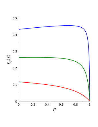
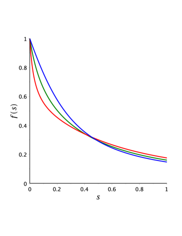
Figure 5: The left panel gives plots of $r_{0}(s)$ versus $p$ for $s=0.2$ in red, $s=0.4$ in green, and $s=0.6$ in blue, respectively. The right panel gives plot of $f(s)$ versus $s$ for $p=0.2$ in red, $p=0.4$ in green, and $p=0.6$ in blue, respectively. Here, $t=1$, $\omega_{0}=0.1$, $\omega_{1}=0.3$, $\delta=3$, $\lambda_{0}=8$, $\mu_{0}=4$, $\mu_{1}=\mu_{0}\omega_{1}/\omega_{0}=12$ and $\lambda_{1}=0$.

$$r_{0}(s) =E(R_{0}|R_{0}<s,V_{0}>R_{0},V_{1}>s-R_{0})$$

$$=\frac{E(R_{0},\,R_{0}<s,V_{0}>R_{0},V_{1}>s-R_{0})}{P(R_{0}<s,V_{0}>R_{0},V_{1}>s-R_{0})}.$$

The expectation simplifies as

$$E (R_{0},\,R_{0}<s,V_{0}>R_{0},V_{1}>s-R_{0})$$

$$=\frac{\lambda}{\lambda+p\delta}\,E(R,\,R<s,V_{0}>R,V_{1}>s-R)$$

$$=\frac{\lambda}{\lambda+p\delta}\,\int_{0}^{s}re^{-\mu_{0}r}e^{-\mu_{1}(s-r)}(1-p)\delta e^{-(1-p)\delta r}\,dr.$$

Furthermore,

$$P (R_{0}<s,V_{0}>R_{0},V_{1}>s-R_{0})$$

$$=\frac{p\delta}{\lambda+p\delta}P(V_{1}>s)+\frac{\lambda}{\lambda+p\delta}\,P(R<s,V_{0}>R,V_{1}>s-R)$$

$$=\frac{p\delta e^{-\mu_{1}s}}{\lambda+p\delta}+\frac{\lambda}{\lambda+p\delta}\int_{0}^{s}e^{-\mu_{0}r-\mu_{1}(s-r)}(1-p)\delta e^{-(1-p)\delta r}dr,$$

and hence, recalling that $\mu=\mu_{0}+(1-p)\delta$,

$$r_{0}(s)=\frac{\lambda(1-p)\int_{0}^{s}re^{(\mu_{1}-\mu)r}\,dr}{p+\lambda(1-p)\int_{0}^{s}e^{(\mu_{1}-\mu)r}\,dr},$$

or, evaluating the integrals,

$$r_{0}(s)=\frac{\lambda(1-p)\Big{(}(\mu_{1}-\mu)s-1+e^{-(\mu_{1}-\mu)s}\Big{)}}{p(\mu_{1}-\mu)^{2}e^{-(\mu_{1}-\mu)s}+\lambda(1-p)(\mu_{1}-\mu)(1-e^{-(\mu_{1}-\mu)s})}.$$ (3.18)

Figure 5 (left panel) shows how $r_{0}(s)$ varies with $p$ for different values of $s$, when $\lambda_{1}=0$. In particular, it can be seen that when changes are not purely cladogenetic ($p<1$), a substantial fraction of the branch evolves as trait-$0$.

Define $f(s)$ to be the fraction of type-$1$, in an observed trait-$0$/trait-$1$ species pair, that is,

$$f(s)\coloneqq\frac{s-r_{0}(s)}{s}.$$

Figure 5 (right panel) gives an illustration of $f(s)$ versus $s$ for different values of $p$, with $\lambda_{1}=0$. It can be seen that $f(s)$ decreases with $s$ whenever $\mu_{1}>\mu=\mu_{0}+(1-p)\delta$. This means that proportionally, the longer the branch leading to type-$1$, the more recent the transition event would be.

Trait-0 Tree Conditioned on the number of Species

Here, we compare the properties of the $0$-species tree derived previously under the assumption of non-extinction at a fixed time, $K_{t}>0$, to the corresponding properties assuming a fixed number of trait-$0$ species at time $t$, $K_{t}=n$. This apart, the setting is the same, and hence the single-type linear branching process $(K_{t})_{t\geq 0}$, $K_{0}=1$, representing the number of trait-$0$ species, has splitting rate $\lambda=\lambda_{0}$ and extinction rate $\mu=\mu_{0}+(1-p)\delta$ restricted to the critical or supercritical case, $\gamma_{0}=\lambda-\mu\geq 0$. Let $t$ be fixed and condition on $K_{t}=n$.

Given $n$ trait-$0$ species at time $t$, the $n-1$ bifurcation times, $S_{1},\dots,S_{n-1}$, are the time intervals from the tips of the tree at $t$ backwards until two species merge. The bifurcation times of the full tree are the same as the bifurcation times of the reduced tree, given $K_{t}=n$. As an alternative, we may think of the tree starting at the time of the most recent ancestor, and scale the tree on the interval $[0,t]$. In both cases, it turns out that the joint distribution of the bifurcation times is the same as that of $n-1$ i.i.d. observations sampled from a particular family of distribution functions $F_{t}(s)$, $0\leq s\leq t$, depending on $\lambda$ and $\mu$ ([26]; [5]). For the supercritical case, $\mu<\lambda$,

$$F_{t}(s)=\frac{\lambda-\mu e^{-\gamma_{0}t}}{1-e^{-\gamma_{0}t}}\,\frac{1-e^{-\gamma_{0}s}}{\lambda-\mu e^{-\gamma_{0}s}},\quad 0\leq s\leq t,$$ (3.19)

and for the critical case, $\mu=\lambda$,

$$F_{t}(s)=\frac{(1+\lambda)s}{t+\lambda s},\quad f(t)=\frac{(1+\lambda)t}{(t+\lambda s)^{2}},\quad 0\leq s\leq t.$$ (3.20)

Writing $S_{(k)}$, $1\leq k\leq n-1$, for the ordered bifurcation times of the reduced type-$0$ tree and adding $S_{(0)}=0$ and $S_{(n)}=t$, so that

$$0=S_{(0)}\leq S_{(1)}\leq\dots\leq S_{(n-1)}\leq S_{(n)}=t,$$

it follows that total branch length $A_{t}$ in (3.1) has the representation

$$A_{t} =n(S_{(1)}-S_{(0)})+(n-1)(S_{(2)}-S_{(1)})+\dots+1\cdot(S_{(n)}-S_{(n-1)})$$

$$=S_{(1)}+S_{(2)}+\dots+S_{(n-1)}+t$$

$$=S_{1}+S_{2}+\dots+S_{n-1}+t.$$

Hence

$$E(A_{t}|K_{t}=n)=(n-1)E[S]+t,$$ (3.21)

where

$$E(S)=\int_{0}^{t}(1-F_{t}(s))\,ds,$$ (3.22)

is obtained from (3.19) or (3.20). We may also use the speciation times

$$T_{k}=t-S_{n-k},\quad T_{(k)}=t-S_{(n-k)},\quad k=0,\dots,n-1,$$

as an alternative to bifurcation times. The ordered speciation times $T_{(k)}$, starting at $T_{(0)}=0$, are the successive branch time points of the reduced tree $\widetilde{K}_{s,t}$ conditioned on $\widetilde{K}_{t,t}=K_{t}=n$. Here, all $T_{k}$, $1\leq k\leq n-1$, are independent and identically distributed with distribution function

$$G_{t}(s)=P(T_{k}\leq s)=P(S>t-s)=1-F_{t}(t-s)=\frac{\gamma_{0}}{\lambda e^{\gamma_{0}(t-s)}-\mu}\frac{1-e^{-\gamma_{0}s}}{1-e^{-\gamma_{0}t}}.$$

Also,

$$E(\widetilde{K}_{s,t}|K_{t}=n)=1+E(\sum_{k=1}^{n-1}1_{\{T_{k}\leq s\}})=1+\sum_{k=1}^{n-1}P(T_{k}\leq s)=1+(n-1)G_{t}(s)$$ (3.23)

is consistent with (3.21) in the form

$$E(A_{t}|K_{t}=n)=\int_{0}^{t}(1+(n-1)G_{t}(s))\,ds=t+(n-1)\int_{0}^{t}\frac{\gamma_{0}}{\lambda e^{\gamma_{0}(t-s)}-\mu}\frac{1-e^{-\gamma_{0}s}}{1-e^{-\gamma_{0}t}}\,ds.$$ (3.24)

An Illustration Using Arbitrary Parameters

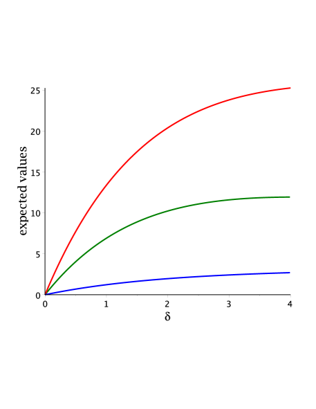
Figure 6: Plot of $E(L_{t}|K_{t}>0)$ versus $\delta$ in red; $E(C_{t}|K_{t}>0)$ versus $\delta$ in green; and $E(B_{t}|K_{t}>0)$ versus $\delta$ in blue. Here, $p=0.5$, $t=1$, $\omega_{0}=0.1$, $\omega_{1}=0.3$, $\lambda_{0}=8$, $\mu_{0}=4$, $\lambda_{1}=10$, $\mu_{1}=z\mu_{0}=12$ and $\mu=4+(1-p)\delta$.

To illustrate the species tree model, we first notice that the trait-$0$ tree, corresponding to the blue colored sub-tree $\mathcal{T}^{0}$ in Figure 2b, only depends on the parameters $\lambda$ and $\mu$. In particular, the expected number of such species at $t$, given at least one existing species, is given by (3.4) as

$$E(K_{t}|K_{t}>0)=\frac{\lambda e^{(\lambda-\mu)t}-\mu}{\lambda-\mu}.$$

Moreover, the expected branch length of the reduced tree, corresponding to the blue-colored subtree $(\mathcal{T}^{0})_{t}$ in Figure 3c, is obtained in (3.6), as

$$E(A_{t}|K_{t}>0)=\int_{0}^{t}\frac{\lambda e^{(\lambda-\mu)t}-\mu}{\lambda e^{(\lambda-\mu)(t-s)}-\mu}\,ds.$$

In case we are given $A_{t}=n$, then according to (3.24) the expected branch length equals

$$E(A_{t}|K_{t}=n)=t+\frac{n-1}{1-e^{-\gamma_{0}t}}\int_{0}^{t}\frac{\gamma_{0}(1-e^{-\gamma_{0}s})}{\lambda e^{\gamma_{0}(t-s)}-\mu}\,ds.$$

In order to comment on the functionals relating to the full tree, let us take a fixed value of the probability $p$ of cladogenetic speciation and assume that the mutation rates $\omega_{0}$ and $\omega_{1}$ are known. Assuming now that point estimates of the parameters $\lambda$ and $\mu$ are known, it means that the trait-$0$ splitting rate $\lambda_{0}=\lambda$ is known whereas the trait-$1$ splitting rate $\mu_{0}=\mu-(1-p)\delta$ is given as a function of $\delta$. The model assumption (2.5) implies moreover that the ratio

$$z=\frac{\mu_{1}}{\mu_{0}}=\frac{\omega_{1}}{\omega_{0}}$$

is known, and therefore $\mu_{1}=z\mu-z(1-p)\delta$ is also a function of $\delta$. Various trait-$1$ functionals may now be studied at a fixed time $t$ of observation as functions of $\delta$ and the remaining parameter $\lambda_{1}$. For a set of arbitrary parameters $p$, $\lambda_{0}$, $\mu_{0}$, $\omega_{0}$, $\omega_{1}$, and $\lambda_{1}$, Figure 6 gives plots of the three functionals, which we will later use to match with data, illustrating the dependence on the trait transition intensity $\delta$.

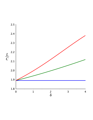
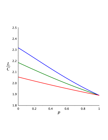
Figure 7: The left panel gives plots of the ratio $L/C=E(L_{t}|K_{t}>0)/E(C_{t}|K_{t}>0)$ versus $\delta$ for $p=0$ in red, $p=0.5$ in green, and $p=1$ in blue, respectively. The right panel gives plots of the ratio $L/C$ versus $p$ for $\delta=1.5$ in red, $\delta=2.5$ in green, and $\delta=3.5$ in blue, respectively. Here, $t=1$, $\omega_{0}=0.1$, $\omega_{1}=0.3$, $\lambda_{0}=8$, $\mu_{0}=4$ and $\lambda_{1}=10$.

Using the same set of arbitrary parameters as in Figure 6, we now obtain plots of the ratio $E(L_{t}|K_{t}>0)/E(C_{t}|K_{t}>0)$ as a function of $p$ and $\delta$. For convenience, we use the shorthand notation $L/C$ to denote this ratio. Plots of $L/C$ as a function of $\delta$, for fixed values of $p$, are shown in left panel of Figure 7. Similarly, plots of $L/C$ versus $p$, for selected values of $\delta$, are given in right panel of Figure 7. As shown in (3.15), it can be seen that for any value of $p$ and $\delta$, the expected number of trait-$1$ species per cluster lies within a given bound. The upper bound is conservative, and for a wide range of arbitrary parameter values, $L/C$ remains closer to the lower bound, meaning that is is unlikely to observe large clades of trait-$1$ species.

4 Application to $dN/dS$

In this section, for convenience, we refer to trait-$0$ as outcrosser and trait-$1$ as selfer. The $dN/dS$-ratio measures the normalized ratio of nonsynonymous to synonymous substitutions. The total mutation intensity splits in two contributions, $\theta=\theta_{\mathrm{syn}}+\theta_{\mathrm{non}}$. The precise fractions $\theta_{\mathrm{syn}}$, representing synonymous mutations and $\theta_{\mathrm{non}}$, nonsynonymous mutations, can be obtained from a detailed mutation model [17] or estimated from data. In the long run, synonymous substitutions build up neutrally at scaled rate $\theta_{\mathrm{syn}}$. The substitution rate of nonsynonymous mutations, on the other hand, is reduced by sligthly deleterious selection to $\omega_{0}\theta_{\mathrm{non}}$ for outcrossing species and to $\omega_{1}\theta_{\mathrm{non}}$ for selfers, $\omega_{0}<\omega_{1}<1$. If we observe a single outcrossing species known to exist over a fixed time duration $t$, the expected number of substitutions are $\theta_{\mathrm{non}}\omega_{0}t$ and $\theta_{\mathrm{syn}}t$ for the two categories, and we understand the normalized ratio to be simply $\omega_{0}$. Similarly, for a species known to have been selfing over a fixed time interval, the corresponding ratio is $\omega_{1}$.

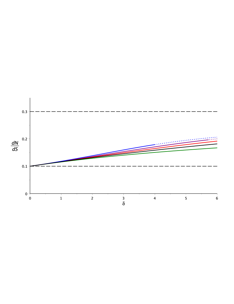
Figure 8: Plots of $dN/dS$ versus $\delta$ for selected values of $p$. The blue curve is obtained for $p=0$; purple for $p=0.3$; red for $p=0.5$; black for $p=0.7$; and green for $p=1$. Here, $t=1$, $\omega_{0}=0.1$, $\omega_{1}=0.3$, $\lambda_{0}=8$, $\mu_{0}=4$ and $\lambda_{1}=10$. The dashed black lines represent the value of $\omega_{0}$ and $\omega_{1}$. The dotted curves give those values of $dN/dS$ which are obtained for a sub critical process (that is, when $\gamma_{0}<0$).

To capture in more detail, the accumulation of fixed mutations in the species tree, we run independent Poisson processes along the branches. First, a collection of Poisson points $\mathcal{S}$ with intensity $\theta_{\mathrm{syn}}$ placed on top of the entire tree, represents synonymous substitutions. Next, nonsynonymous substitutions are generated by a Poisson measure $\mathcal{N}^{(0)}$ with intensity $\omega_{0}\theta_{\mathrm{non}}$ along all outcrossing branches, and by a measure $\mathcal{N}^{(1)}$ with intensity $\omega_{1}\theta_{\mathrm{non}}$ along the branches representing selfers. The random variable $\mathcal{S}_{t}=\mathcal{S}(\mathcal{T}_{t})$ counts the number of synonymous substitutions in the species tree reduced at $t$. Thus,

$$\mathcal{S}_{t} =\mbox{$\#$ accumulated synonymous substitutions in all existing species at $t$},\quad t\geq 0,$$

is a Poisson process modulated by the stochastic intensity $\theta_{\mathrm{syn}}\,(A^{\prime}_{t}+B_{t})$. Indeed, conditionally, given $t$ and given the total branch lengths $A^{\prime}_{t}$ and $B_{t}$ of outcrossers and selfers in the reduced tree, introduced in (3.2) and (3.3), $\mathcal{S}_{t}$ has a Poisson distribution with mean $\theta_{\mathrm{syn}}(A^{\prime}_{t}+B_{t})$. Similarly,

$$\mathcal{N}^{(i)}_{t} =\mbox{$\#$ nonsynonymous substitutions of type-$i$ up to time $t$},\quad i=0,1,$$

are Poisson processes modulated by the random intensities $\theta_{\mathrm{non}}\omega_{0}\,A^{\prime}_{t}$ and $\theta_{\mathrm{non}}\omega_{1}\,B_{t}$, respectively.

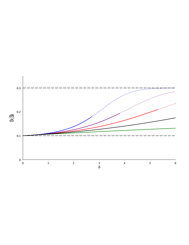
Figure 9: Plots of $dN/dS$ versus $\delta$ for selected values of $p$. The blue curve is obtained for $p=0$; purple for $p=0.3$; red for $p=0.5$; black for $p=0.7$; and green for $p=1$. Here, $t=1$, $\omega_{0}=0.1$, $\omega_{1}=0.3$, $\lambda=8$, $\mu=6$ and $\lambda_{1}=10$. The dashed black lines represent the value of $\omega_{0}$ and $\omega_{1}$. The dotted curves are those values of $dN/dS$ which are not compatible with the biological assumptions (that is, when $r_{1}>0$). In this example, the trait-$0$ tree parameters, $\lambda$ and $\mu$, are fixed, and these give $E(A_{1}|K_{1}>0)\approx 5.7$. Hence, the outcrosser tree is preserved.

In our context, it is natural to associate $dN/dS$ with the average number of substitutions, which have occurred anywhere in the species family tree and are observable today. Substitutions observable today must have occurred on the reduced tree. Of course, a meaningful $dN/dS$ concept is naturally conditioned on survival of some species today. This leads us to considering the $dN/dS$-ratio

$$dN/dS \sim\frac{(E(\mathcal{N}_{t}^{(0)}|K_{t}>0)+E(\mathcal{N}_{t}^{(1)}|K_{t}>0)/\theta_{\mathrm{non}}}{E(\mathcal{S}_{t}|K_{t}>0)/\theta_{\mathrm{syn}}}$$

$$=\frac{\omega_{0}E(A^{\prime}_{t}|K_{t}>0)+\omega_{1}E(B_{t}|K_{t}>0)}{E(A^{\prime}_{t}+B_{t}|K_{t}>0)}.$$

The conditioning scheme of assuming at least one outcrosser at $t$, $K_{t}>0$, is to some degree, arbitrary. Alternatives, such as assuming $K_{t}=k$ or imposing a condition involving both $K_{t}$ and $L_{t}$, are equally natural. Our choice is computationally more convenient and hence we define

$$dN/dS|_{t}=\frac{\omega_{0}E(A^{\prime}_{t}|K_{t}>0)+\omega_{1}E(B_{t}|K_{t}>0)}{E(A^{\prime}_{t}|K_{t}>0)+E(B_{t}|K_{t}>0)}.$$

Typically it is straightforward to estimate the total branch length in the denominator, given by

$$T_{\mathrm{tot}}=E(A^{\prime}_{t}|K_{t}>0)+E(B_{t}|K_{t}>0),$$

and also the ratio

$$q^{0}_{t}=\frac{E(A_{t}|K_{t}>0)}{E(A^{\prime}_{t}|K_{t}>0)+E(B_{t}|K_{t}>0)},$$ (4.1)

while the desired ratio of expected values is

$$q_{t}=\frac{E(A^{\prime}_{t}|K_{t}>0)}{E(A^{\prime}_{t}|K_{t}>0)+E(B_{t}|K_{t}>0)}\geq q^{0}_{t},$$ (4.2)

for which

$$dN/dS|_{t}=q_{t}\omega_{0}+(1-q_{t})\omega_{1}.$$

The value of $q_{t}$ in (4.2) may be be computed when $\lambda_{1}=0$, since in this case, $E(A^{\prime}_{t}|K_{t}>0)$ can be obtained using (3.17).

For $t=1$, fixed mutation rates $\omega_{0}$ and $\omega_{1}$, and arbitrary values of parameters $\lambda_{0}$, $\mu_{0}$, and $\lambda_{1}$, Figure 8 illustrates the shape of $dN/dS$ versus $\delta$, for selected values of $p$. Here, $\mu_{1}=\mu_{0}\omega_{1}/\omega_{0}$ is fixed, whereas $\mu$, obtained by using the relation $\mu=\mu_{0}+(1-p)\delta$, varies with $p$ and $\delta$. Figure 9 shows similar types of plots, obtained by using the same parameters as in Figure 8, except that here, $\mu$ is fixed, while $\mu_{0}=\mu-(1-p)\delta$ and $\mu_{1}=\mu_{0}\omega_{1}/\omega_{0}$ are allowed to vary with $p$ and $\delta$. Since the values of $\lambda$ and $\mu$ are fixed in Figure 9, the outcrosser tree remains preserved in this case.

5 Relating Model to Species Tree Data

This section discusses how to relate our theoretical study of random species trees to given data sets from two plant families, Geraniaceae and Solanaceae, in order to provide a first test of the relevance of the mathematical modeling. In each case, a sequence data set is available for an observed selfer-outcrosser species family of total size $m$, consisting of $k$ outcrossing and $l$ selfing species, such that $k+l=m$. The data set for the Geraniaceae family has a known outgroup that helps placing the origin of the family. For the Solanaceae data set, the outgroup information is missing, and hence we insert a virtual root for the tree.

Geraniaceae Family

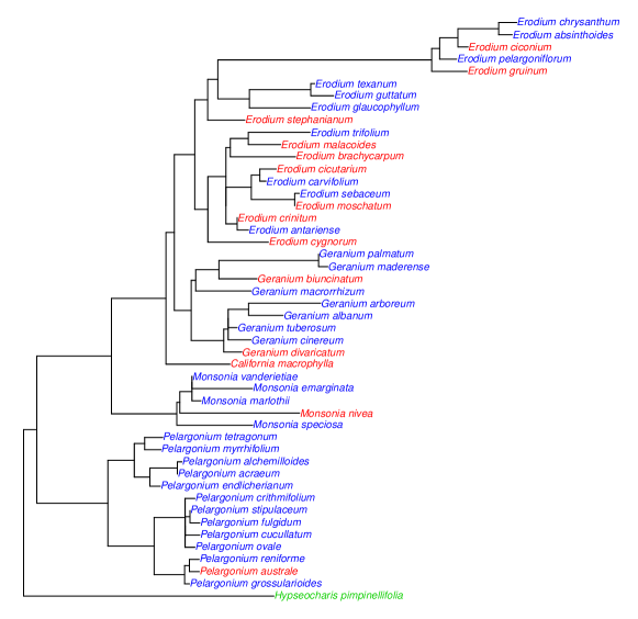
Figure 10: Phylogenetic tree consisting of $47$ species in the Geraniaceae family and the outgroup. Outcrossers are colored in blue, selfers in red, and the outgroup in green.

The sequence data set for the Geraniaceae family, obtained from [6], consists of $1425$ codons in an interleaved format, a known outgroup, and $m=47$ species, of which $k=33$ are outcrossers and $\ell=14$ are selfers.

1. Estimating the tree characteristics.—

The phylogeny analysis software PhyML [10], with nucleotide substitution model GTR, branch support set to aLRT, BIONJ starting tree, and tree searching operation NNI, was used to construct the phylogenetic tree, which is given in Figure 10. The program PAML [28] was used to obtain $Q=0.0955$, defined as the estimate of the global $dN/dS$ ratio over the whole tree (excluding the outgroup). The outcrosser species sub-tree, was then obtained by removing all selfing branches from the initial tree in Figure 10. PAML was used on this outcrosser sub-tree and the corresponding sequence data, which yielded the $dN/dS$-value, essentially an estimate of $\omega_{0}$, as $\omega_{0}=0.075$. The observed ordering $\omega_{0}<Q$ is consistent with our basic hypothesis that $\omega_{0}\leq\omega_{1}$.

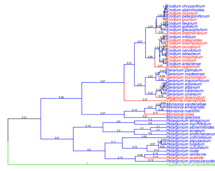
Figure 11: Ultrametric phylogenetic tree consisting of $47$ species in the Geraniaceae family and the outgroup. Outcrosser branches are colored blue; the selfer branches, from bifurcation time onward, are given in red; the outgroup branch is colored in green, and the ‘virtual’ outcrosser branch in black. The numbers on each branch represent the branch length.

The tree in Figure 10 was then made ultrametric with the function ‘chronos’ of the package ‘ape’ [20] in the software R [21], and normalized to have $t=1$. This ultrametric tree is given in Figure 11. The length of the branch, leading from the root of the tree to the first speciation time, was estimated using the outgroup species, and can be considered a ‘virtual’ branch length, used to match the mathematical model to our phylogenetic analysis. The total branch length of the tree, excluding the outgroup, is $T_{\mathrm{tot}}=6.926$. By removing selfing branches from the ultrametric tree in Figure 11, the ultrametric version of the outcrossing sub-tree at time $t$ was also obtained, as given in Figure 12. From this outcrossing sub-tree, corresponding to $(\mathcal{T}^{0})_{t}$, we record: (a) the observed ordered bifurcation times $0\leq s_{(1)}\leq\dots\leq s_{(n-1)}\leq s_{(n)}=t$, given in Fig. 12; (b) the observed total branch-length

$$T^{(0)}_{\mathrm{tot}}=s_{(1)}+\dots+s_{(n)}=6.045;$$

and, (c) the sample mean of the bifurcation times

$$\bar{s}=(s_{(1)}+\dots+s_{(n-1)})/(n-1)=0.1577.$$

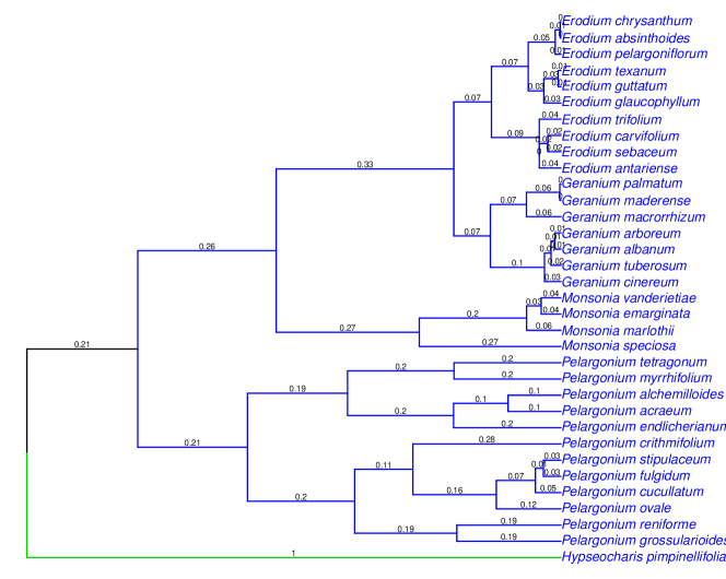
Figure 12: Ultrametric outcrosser tree consisting of $33$ species in the Geraniaceae family and the outgroup. Outcrosser branches are in blue, the outgroup branch in green, and the virtual outcrosser branch is colored black. The number given on each branch represents the branch’s length.

2. Obtaining the lower bound for $\omega_{1}$.—

The quotient

$$q^{0}=T^{(0)}_{\mathrm{tot}}/T_{\mathrm{tot}}=0.873$$

is a numerical estimate of the ratio in (4.1), interpreted as the minimal fraction of outcrossing branches in the full species tree. Since $Q$ is a point estimate of $dN/dS|_{1}$, we have

$$Q=q\omega_{0}+(1-q)\omega_{1},\quad q\geq q^{0}$$ (5.1)

where $q$ is the actual fraction of outcrossing branches in the full tree. In view of (5.1), with $Q$ and $\omega_{0}$ both known, $\omega_{1}$ is an increasing function of $q$, and hence we have the lower bound

$$\omega_{1}=\frac{Q-\omega_{0}q}{1-q}\geq\frac{Q-\omega_{0}q^{0}}{1-q^{0}}=0.236,\quad q\geq q^{0}.$$ (5.2)

3. Estimating the outcrosser parameters, $\lambda$ and $\mu$.—

We list three methods for extracting admissible pairs $(\lambda,\mu)$ consistent with data. By combining these methods, the parameter space is further reduced, leading to reasonable estimates of the separate parameters $\lambda$ and $\mu$. The methods are

i) Use $k=33$ as a point estimate of $E(K_{t}|K_{t}>0)$ at $t=1$. By (3.4), this gives

$$\frac{\lambda e^{(\lambda-\mu)}-\mu}{\lambda-\mu}=33.$$ (5.3)

ii) Apply the relation (3.22) using $\bar{s}=0.1577$ as an estimate of $E(S)$, that is, estimate $(\lambda,\mu)$ from

$$\int_{0}^{1}(1-F_{1}(s))\,ds=\int_{0}^{1}\big{(}1-\frac{\lambda-\mu e^{-\gamma_{0}}}{1-e^{-\gamma_{0}}}\,\frac{1-e^{-\gamma_{0}s}}{\lambda-\mu e^{-\gamma_{0}s}}\Big{)}\,ds=0.1577.$$ (5.4)

iii) Apply the branch length statistics $T^{(0)}_{\mathrm{tot}}=6.045$ as an approximation for $E(A_{t}|K_{t}>0)$ at $t=1$ obtained in (3.6), and hence solve for $(\lambda,\mu)$ as

$$\int_{0}^{1}\frac{\lambda e^{\gamma_{0}}-\mu}{\lambda e^{\gamma_{0}s}-\mu}\,ds=6.045.$$ (5.5)

The $(\lambda,\mu)$ pairs obtained numerically in each of the three cases are plotted in Figure 13. By comparing the three estimation methods, we obtain the parameter estimates $\lambda\approx 10.462$ and $\mu\approx 8.526$. Figure 14 (left panel) shows that the empirical distribution of the bifurcation times $(s_{1},\dots,s_{32})$ of the ultrametric outcrosser tree, fits rather well the distribution function $F_{1}(s)$, $0\leq s\leq 1$, of the supercritical birth and death model in (3.19), when $\lambda=10.462$ and $\mu=8.526$. Similarly, Figure 14 (right panel) gives a plot of the number of species in the ultrametric outcrosser tree, along with a plot of the expected values in (3.23), when $\lambda=10.462$ and $\mu=8.526$.

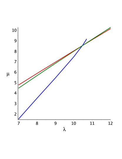
Figure 13: Numerical solutions for method i) plotted in green, for method ii) in blue, and for method iii) in red. The three lines approximately meet at a point where $\lambda=10.462$ and $\mu=8.526$.

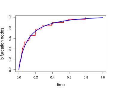
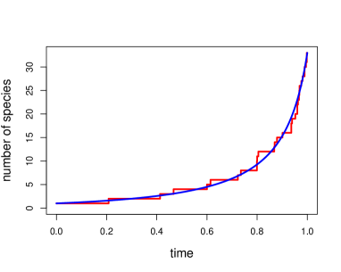
Figure 14: In the left panel, the red plot gives the empirical distribution of the bifurcation times $(s_{1},\dots,s_{32})$ of the tree given in Figure 12 and the blue graph is a plot of (3.19) with $t=1$, $\lambda=10.462$ and $\mu=8.526$. In the right panel, the red graph is a plot of the number of species versus time for the tree given in Figure 12 and the blue graph is a plot of (3.23) with $t=1$, $\lambda=10.462$ and $\mu=8.526$.

4. Estimating the selfer species rates.—

By the definition of $q$, and using (5.1), the expected selfer branch length equals

$$E(B_{1}|K_{1}>0)=(1-q)T_{\mathrm{tot}}=\frac{Q-\omega_{0}}{\omega_{1}-\omega_{0}}T_{\mathrm{tot}}.$$ (5.6)

Also, by (2.5), and using the rate of removal of outcrossers ($\mu=\mu_{0}+(1-p)\delta$), the exinction rate, $\mu_{1}$, of selfers is a function of $p$, $\delta$, and $\omega_{1}$,

$$\mu_{1}=\frac{\omega_{1}}{\omega_{0}}\,\mu_{0}=\frac{\omega_{1}}{\omega_{0}}(\mu-(1-p)\delta).$$ (5.7)

The Geraniaceae data set has the particular feature that the number of selfing species coincides with the number of selfing clusters, both $14$. In other words, each observed selfer, at $t=1$, is joined to an outcrosser, at the most recent bifucation point. In particular, using (3.16), we infer the estimate $\lambda_{1}=0$.

Now, by rewriting (3.11) and (3.12) for $t=1$ and $\lambda_{1}=0$, we obtain

$$E(B_{1}|K_{1}>0)=\delta\int_{0}^{1}\int_{0}^{s}E(K_{u}|K_{1}>0)e^{-\mu_{1}(1-u)}duds.$$ (5.8)

The right hand side of (5.8) equated to the right hand side of (5.6) gives

$$\delta\int_{0}^{1}\int_{0}^{s}E(K_{u}|K_{1}>0)e^{-\mu_{1}(1-u)}duds=\frac{Q-\omega_{0}}{\omega_{1}-\omega_{0}}T_{\mathrm{tot}},$$ (5.9)

where $E(K_{u}|K_{1}>0)$ is obtained in (3.9).

Similarly, (3.8) and (3.10) can be rewritten for $t=1$ and $\lambda_{1}=0$, as

$$E(L_{1}|K_{1}>0)=\delta\int_{0}^{1}E(K_{s}|K_{1}>0)e^{-\mu_{1}(1-s)}\,ds.$$ (5.10)

Making the identification $E(L_{1}|K_{1}>0)=\ell=14$, we obtain from the right hand side of (5.10)

$$\delta\int_{0}^{1}E(K_{s}|K_{1}>0)e^{-\mu_{1}(1-s)}\,ds=14,$$ (5.11)

where $E(K_{s}|K_{1}>0)$ is obtained in (3.9), as before.

Furthermore, by invoking relation (3.17), valid for $\lambda_{1}=0$, we have the estimate $\hat{q}$ of $q$, given by

$$\hat{q}=q^{0}+\frac{1}{T_{\mathrm{tot}}}\sum_{i=1}^{\ell}r_{0}{(s_{i})},$$

where the selfer bifurcation times, $s_{i}=(s_{1},\dots,s_{14})$, are shown in Figure 11 and $r_{0}{(s_{i})}$, $i=1\dots 14$, are obtained in (3.18). Here, $\sum_{i}s_{i}=0.881$ whereas $T^{(1)}_{\mathrm{tot}}=0.881-\sum_{i}r_{0}{(s_{i})}$ is the total expected branch length represented by selfers. Now, each $(p,\delta,\omega_{1})$ gives a $\hat{q}$. On the other hand, each $\hat{q}$ yields an $\omega_{1}$, using

$$\hat{\omega}_{1}=\frac{Q-\hat{q}\omega_{0}}{1-\hat{q}}.$$ (5.12)

5. Estimating the parameters $p$, $\delta$ and $\omega_{1}$.—

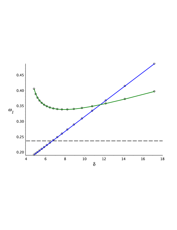
Figure 15: Plot of $\omega_{1}$ versus $\delta$ with fixed $p$-values. The blue graph represents pairs $(\omega_{1},\delta)$ satisfying (5.9) and (5.11). The green graph represents $(\omega_{1},\delta)$ pairs which satisfy (5.12). The circular marks on both graphs are successive $p$-values $0,0.05,0.10,\dots,0.85$. The dashed line marks the lower bound for $\omega_{1}$.

For any fixed $p$, we are now in position to find admissible pairs $(\omega_{1},\delta)$ which satisfy the two equations (5.9) and (5.11). These pairs are plotted as the blue line in Figure 15, with successive $p$-values indicated as circles along the line starting from the lower left. It is seen that all solutions with $p>0.39$ are consistent with the bound $\omega_{1}\geq 0.236$ obtained in (5.2). By going through the $p$-values once more, however, and evaluating $\hat{\omega}_{1}$ according to (5.12), one obtains the green line in Figure 15. At the crossing point of the blue and green curves, a unique combination of parameters, which satisfy all criteria set up in this analysis, are obtained. These are $p=0.732$, $\omega_{1}=0.353$, and $\delta=11.623$.

6. Conclusions—

As a final result, we obtain the following branching tree rates

$$\lambda_{0}=\lambda=10.462,\quad\lambda_{1}=0,\quad\mu_{0}=5.411,\quad\mu=8.526,\quad\mu_{1}=25.468,$$

$$\delta=11.623,\quad p=0.732.$$

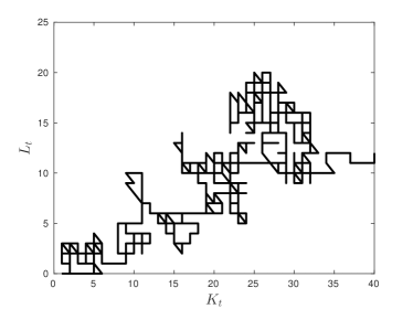
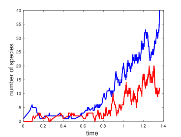
Figure 16: Simulation of a two-type branching process with $\omega_{0}=0.075$, $\omega_{1}=0.353$, $\lambda_{1}=0$, $\lambda=10.462$, $\mu=8.526$, $p=0.732$, $\delta=11.623$, $\mu_{0}=5.411$ and $\mu_{1}=25.468$. The left plot gives the trace of $(K_{t},L_{t})$ in the $(k,\ell)$ plane; Plot on the right shows the paths over time of $K_{t}$ and $L_{t}$ in blue and red, respectively.

These are linked to the mutation rates

$$\omega_{0}=\frac{\mu_{0}}{c}=0.075,\quad\omega_{1}=\frac{\mu_{1}}{c}=0.353,\quad c=72.147,$$

such that, at time $t=1$,

$$dN/dS|_{1}=q\omega_{0}+(1-q)\omega_{1}=0.0955,\quad q=0.9263.$$

The corresponding two-type branching process is supercritical with extinction probability $\mu/\lambda=0.815$. Figure 16 shows a fairly typical realization of the branching process, conditional on non-extinction. Left panel of Figure 16 gives the trace of $(K_{t},L_{t})$ in the $(k,\ell)$ plane, whereas the right panel shows the paths over time of $K_{t}$ and $L_{t}$.

Solanaceae Family

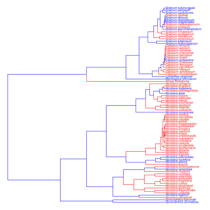
Figure 17: Ultrametric phylogenetic tree consisting of $83$ species in the Solanaceae family. Outcrosser branches are colored blue; the selfer branches, from bifurcation time onward, are given in red.

The data set for the Solanaceae family, obtained from [6], consists of a total of $1527$ codons in an interleaved format and $m=83$ species ($k=22$ outcrossers and $\ell=61$ selfers). The selfing species form $25$ separate clusters. The corresponding phylogenetic tree is given in Figure 17.

It is straightforward to repeat all steps $1-3$ outlined in the previous section. The $dN/dS$-ratio of the complete species tree at $t=1$, is observed to be $Q=0.439$, whereas the estimated $dN/dS$-value restricted to outcrossers is $\omega_{0}=0.4206$. The ultrametric version (Fig. 17) of the phylogenetic tree, when the ‘virtual’ root length is set at $0.1$, has total branch length $T_{\mathrm{tot}}=7.881$. The sum of all outcrossing branch lengths (including the root) is $T^{(0)}_{\mathrm{tot}}=4.845$. Hence, the minimal fraction of outcrossers is approximately $q^{0}=0.615$ and therefore, as in (5.2),

$$\omega_{1}\geq\frac{Q-\omega_{0}q^{0}}{1-q^{0}}=0.468.$$

The estimation of admissible pairs $(\lambda,\mu)$ proceeds by applying the following methods.

i) Use (5.3) with $k=22$ as

$$\frac{\lambda e^{(\lambda-\mu)}-\mu}{\lambda-\mu}=22.$$

ii) Use (5.4) with $\bar{s}=0.183$, obtained from the bifurcation times $(s_{1},\dots,s_{21})$ of the outcrossing species, that is

$$\int_{0}^{1}(1-F_{1}(s))\,ds$$

$$=\int_{0}^{1}\big{(}1- \frac{\lambda-\mu e^{-\gamma_{0}}}{1-e^{-\gamma_{0}}}\,\frac{1-e^{-\gamma_{0}s}}{\lambda-\mu e^{-\gamma_{0}s}}\Big{)}\,ds=0.183.$$

iii) Use (5.5) with $T^{(0)}_{\mathrm{tot}}=4.845$ as follows

$$\int_{0}^{1}\frac{\lambda e^{\gamma_{0}}-\mu}{\lambda e^{\gamma_{0}s}-\mu}\,ds=4.845.$$

The above three cases give an approximation for $\lambda$ and $\mu$ values, i.e., $\lambda\approx 8.097$ and $\mu\approx 6.417$.

From here on, attempting to estimate the remaining parameters $\omega_{1}$, $p$, $\delta$, and $\lambda_{1}$ (which will give $\mu_{0}$ and $\mu_{1}$), it becomes apparent that the Solanaceae data set does not line up with the branching model as accurately as the Geraniaceae data set did. Our tools rely on measuring the number of selfers, the number of selfing clusters, and the length of selfing branches. Any two of these can be matched to a set of parameters of the branching tree model, but matching all three together seem to be out of range. For example, if we focus on number of selfers and number of clusters, the fraction of selfing branch length, $1-q$, arising in the branching model, will be larger than the fraction accounted for in the observed ultrametric tree. An interpretation of the discrepancy might be that the sequence data set is so restricted that many of the selfers come out biased towards short divergence times. These difficulties remain even if we allow for more flexible conditions than (2.5). As an example, the parameters

$$\mu=13.3,\;\lambda=14.1,\;\lambda_{1}=9.5,\;p=0.25,\;\delta=7.5,\;\mu_{0}=7.675,$$

are consistent with the $dN/dS$ value in selfers, that is $\omega_{1}=0.6$, as well as the correct number of selfers and selfing clusters in the tree. The corresponding two-type branching process is supercritical with extinction probability $\mu/\lambda=0.943$.

6 Discussion

In this paper, we combined trait-dependent diversification models, BiSSE and ClaSSE, with trait-dependent substitution models. We focused on binary-trait models, based on the ‘evolutionary dead-end’ hypothesis, with unidirectional shift from a trait-$0$ to a trait-$1$, where trait-$1$ had a lower diversification rate than trait-$0$. To do so, we first described several properties of the BiSSE and ClaSSE models that have not been obtained before. In particular, we introduced a novel way to decompose and analyze the reduced trait-$0$ and trait-$1$ species trees. We then showed how trait-dependent diversification processes affect the inference and interpretation of relationships between traits and molecular evolutionary rates.

We obtained several expressions describing the tree characteristics, such as the expected branch lengths of the reduced trees as well as their cluster sizes. The expected number of trait-$1$ species per cluster in particular, is biologically relevant; numerical exploration showed that this value stayed within controlled boundaries under a wide range of conditions. Assigning outcrossing and selfing species as trait-$0$ and trait-$1$, respectively, this formally confirms the general observation that large clades of selfing species are rare. Larger clusters of selfing species can only be obtained for the supercritical case, i.e., if $\lambda_{1}>\mu_{1}$, which corresponds to conditions where selfing is no more an evolutionary dead-end.

A specially interesting case occurs when selfing species are only found as singletons, as shown in the Geraniaceae family example. Such a case can be rather frequent – for example it corresponds to $5$ of the $16$ datasets in [6] study – and it allows for a more complete treatment of the problem. In particular, we showed that under this condition, testing the difference of $dN/dS$ between outcrossing and selfing branches can be difficult. For longer branches leading to the selfing species, we could expect to have more power to distinguish between $\omega_{0}$ and $\omega_{1}$, simply because more substitutions occur and $\omega_{0}$, $\omega_{1}$ values are better estimated. However, the proportion of the branch with $\omega_{1}$ decreases as the branch length increases, making $\omega_{0}$ and $\omega_{1}$ values closer to one another. No matter what the conditions may be, assuming a pure cladogenetic model, when it is not, reduces the ability to detect differences in $\omega_{0}$ and $\omega_{1}$ values, either by lack of power (short branches), or, by incorrect trait assignation (long branches). Moreover, for short branches, the mutation substitution process cannot be considered as instantaneous, and the polymorphic transitory phase – currently not included in our modeling framework – must be taken into account to avoid detection of spurious changes in $dN/dS$ [17]. Thus, not detecting any effect of selfing on $dN/dS$ does not necessarily mean that the effect is weak. The same rationale and conclusions can be applied to other binary traits, such as hermaphroditism versus dioecy [14], sexuality versus clonality [11] and solitary life versus sociality [22].

Overall, our results show that trait-dependent diversification processes can have a strong impact on the relationship between traits and molecular evolution. A further step would be to develop statistical methods allowing to jointly infer the effect of traits on both the diversification process and, the molecular evolutionary rates. Here, we propose a straightforward way to connect the two processes by making substitution and extinction rates proportional to one another, but this could be extended to other functions – a linear function of course being a more natural assumption. Allowing for two-sided transitions (reversion from selfing to outcrossing, in our example) would also be a natural extension, but would lead to more complex treatments, since both trait-$0$ and trait-$1$ trees could be disjoint. We hope that the modeling framework presented in our paper, will be a useful starting point for further development in this field of research.

Supplementary Material

The Maple code use to obtain Figures 13 and 15 can be found in the Dryad Digital Repository: http://dx.doi.org/10.5061/dryad.3rg40

Funding

This work was supported by the Marie Curie Intra-European Fellowship (grant number IEF-623486, project SELFADAPT to S.G. and M.L.). D.T. is supported by The Centre for Interdisciplinary Mathematics in Uppsala University.

Appendix 1

This section elaborates the mathematical properties of the two-type, continuous time Markov branching process $X_{t}=(K_{t},L_{t})$, given in (2.1). Here, we analyze the process following the same approach and notation as in [2].

The branching rates of $X_{t}$, given in (2.2), are rewritten below for convenience

$$(k,\ell)\mapsto\left\{\begin{array}[]{cc}(k+1,\ell)&\lambda_{0}k\\ (k-1,\ell+1)&(1-p)\delta k\\ (k-1,\ell)&\mu_{0}k\\ (k,\ell+1)&p\delta k+\lambda_{1}\ell\\ (k,\ell-1)&\mu_{1}\ell.\end{array}\right.$$ (2.2)

The life length of type-$i$, $i=0,1$, is exponentially distributed with parameter $\mathbf{a}=(a_{0},a_{1})$, such that

$$a_{0}=\lambda_{0}+\mu_{0}+\delta\quad\mbox{and}\quad a_{1}=\lambda_{1}+\mu_{1}.$$

The offspring distribution of the two types is given by $\mathbf{p(j)}=(p^{(0)}(\mathbf{j}),p^{(1)}(\mathbf{j}))$, where

$$p^{(0)}(2,0)=\frac{\lambda_{0}}{\lambda_{0}+\delta+\mu_{0}},\quad p^{(0)}(0,1)=\frac{(1-p)\delta}{\lambda_{0}+\delta+\mu_{0}},$$

$$p^{(0)}(0,0)=\frac{\mu_{0}}{\lambda_{0}+\delta+\mu_{0}},\quad p^{(0)}(1,1)=\frac{p\delta}{\lambda_{0}+\delta+\mu_{0}},$$

$$p^{(1)}(0,2)=\frac{\lambda_{1}}{\lambda_{1}+\mu_{1}},\quad\quad p^{(1)}(0,0)=\frac{\mu_{1}}{\lambda_{1}+\mu_{1}},$$

and

$$\sum_{j}p^{(i)}(\mathbf{j})=1.$$

The generating function is of the form $\mathbf{f(s)}=(\mathbf{f}^{(0)}(\mathbf{s}),\mathbf{f}^{(1)}(\mathbf{s}))$, where $\mathbf{f}^{(i)}(\mathbf{s})=\sum_{j}p^{(i)}(\mathbf{j})\mathbf{s}^{j}$, that is

$$f^{(0)}(s_{0},s_{1})=\frac{\lambda_{0}s_{0}^{2}+p\delta s_{0}s_{1}+(1-p)\delta s_{1}+\mu_{0}}{\lambda_{0}+\delta+\mu_{0}},$$

and

$$f^{(1)}(s_{0},s_{1})=\frac{\lambda_{1}s_{1}^{2}+\mu_{1}}{\lambda_{1}+\mu_{1}}.$$

The infinitesimal generating function is given by $\mathbf{u}^{i}(\mathbf{s})=a_{i}[\mathbf{f}^{(i)}(\mathbf{s})-s_{i}]$. Hence,

$$u^{(0)}(s_{0},s_{1})={}\lambda_{0}s_{0}^{2}+p\delta s_{0}s_{1}+(1-p)\delta s_{1}-(\lambda_{0}+\delta+\mu_{0})s_{0}+\mu_{0},$$

and

$$u^{(1)}(s_{0},s_{1})=\lambda_{1}s_{1}^{2}-(\lambda_{1}+\mu_{1})s_{1}+\mu_{1}.$$

The mean offspring matrix $A$ is defined as

$$A=(a_{ij}),\quad\mbox{where}\quad a_{ij}=a_{i}\Big{[}\frac{\partial f^{(i)}(\mathbf{s})}{\partial s_{j}}\Big{|}_{\mathbf{s}=1}-\delta_{ij}\Big{]},$$

and

$$\delta(i,j)=\left\{\begin{array}[]{cc}1\quad\;\;\;\mbox{if}\;\;\quad i=j\\ 0\quad\mbox{otherwise}.\end{array}\right.$$

Hence,

$$A=\left(\begin{array}[]{cc}\lambda_{0}-(1-p)\delta-\mu_{0}&\delta\\ 0&\lambda_{1}-\mu_{1}\end{array}\right).$$

The eigenvalues of $A$,

$$\gamma_{0}=\lambda_{0}-(1-p)\delta-\mu_{0}\quad\mbox{and}\quad\gamma_{1}=\lambda_{1}-\mu_{1},$$

are classified as

$$\gamma_{+}=\max(\gamma_{0},\gamma_{1})\quad\left\{\begin{array}[]{lc}<0&\mbox{subcritical}\\ =0&\mbox{critical}\\ >0&\mbox{supercritical}.\end{array}\right.$$

The extinction probabilities

$$q_{0}=P(\mbox{extinction}|\mbox{starting with one outcrosser}),$$

and

$$q_{1}=P(\mbox{extinction}|\mbox{starting with one selfer}),$$

are the solutions of the system

$$q_{0}=f^{(0)}(q_{0},q_{1}),\quad q_{1}=f^{(1)}(q_{0},q_{1}),$$

or equivalently

$$u^{(0)}(q_{0},q_{1})=0,\quad u^{(1)}(q_{0},q_{1})=0.$$

By solving this system, we obtain

$$q_{0}=\frac{\mu_{0}+(1-p)\delta}{\lambda_{0}}\quad\mbox{and}\quad q_{1}=1.$$

Mean values.—

Given

$$m_{00}(t)=E(K_{t}|K_{0}=1),\quad\;\;\;m_{11}(t)=E(L_{t}|L_{0}=1),$$

$$m_{01}(t)=E(L_{t}|K_{0}=1),\;\;\;m_{10}(t)=E(K_{t}|L_{0}=1)=0,$$

$$M(t)=\left(\begin{array}[]{cc}m_{00}(t)&m_{01}(t)\\ 0&m_{11}(t)\end{array}\right),$$

we have $M(s+t)=M(s)M(t)$ and $M(t)\to I$ as $t\to 0$. Hence $M(t)=e^{At}$, and

$$m_{00}(t)=e^{(r_{0}-(1-p)\delta)t},\quad m_{11}(t)=e^{r_{1}t},$$

$$m_{01}(t)=\frac{\delta}{r_{0}-(1-p)\delta-r_{1}}\big{[}e^{(r_{0}-(1-p)\delta)t}-e^{r_{1}t}\big{]}.$$

Here, $M(t)$ is not positively regular. However,

$$\frac{E(K_{t})}{E(K_{t})+E(L_{t})}=\frac{m_{00}(t)}{m_{00}(t)+m_{01}(t)}\to 1-\frac{\delta}{r_{0}-r_{1}+p\delta},$$

and

$$\frac{E(L_{t})}{E(K_{t})}=\frac{m_{01}(t)}{m_{00}(t)}\to\frac{\delta}{r_{0}-(1-p)\delta-r_{1}},$$

as $t\to\infty$.

References

- [1] Antal T., Krapivsky P.L. 2011. Exact solution of a two type branching process: models of tumor progression. J. Stat. Mech.: Theory Exp. P08018.
- [2] Athreya K.B., Ney P.E. 1972. Branching processes. New York: Springer Verlag Berlin Heidelberg.
- [3] Charlesworth D. 2006. Evolution of plant breeding systems. Curr. Biol. 16:726–735.
- [4] Figuet E., Nabholz B., Bonneau M., Carrio E.M., Brzyska K.N., Ellegren H., Galtier N. 2016. Life history traits, protein evolution, and the nearly neutral theory in amniotes. Mol. Biol. Evol. 33:1517–1527.
- [5] Gernhard T. 2008. The conditioned reconstructed process. J. Theor. Biol. 253:769–778.
- [6] Glémin S., Muyle A. 2014. Mating systems and selection efficacy: a test using chloroplastic sequence data in angiosperms. J. Evol. Biol. 27:1386–1399.
- [7] Goldberg E.E., Igić B. 2008. On phylogenetic tests of irreversible evolution. Evolution 62:2727–2741.
- [8] Goldberg E.E., Kohn J.R., Lande R., Robertson K.A., Smith S.A., Igić B. 2010. Species selection maintains self-incompatibility. Science 330:493–495.
- [9] Goldberg E.E., Igić B. 2012. Tempo and mode in plant breeding system evolution. Evolution 66:3701–3709.
- [10] Guindon S., Gascuel O. 2003. A simple, fast, and accurate algorithm to estimate large phylogenies by maximum likelihood. Syst. Biol. 52:696–704.
- [11] Henry L., Schwander T., Crespi B.J. 2012. Deleterious mutation accumulation in asexual Timema stick insects. Mol. Biol. Evol. 29:401–408.
- [12] Igic B., Lande R., Kohn J.R. 2008. Loss of self incompatibility and its evolutionary consequences. Int. J. Plant Sci. 169:93–104.
- [13] Igic B., Busch J.W. 2013. Is self fertilization an evolutionary dead end? New Phytol. 198:386–397.
- [14] Käfer J., Talianová M., Bigot T., Michu E., Guéguen L., Widmer A., Žluvová J., Glémin S., Marais G.A. 2013. Patterns of molecular evolution in dioecious and non-dioecious Silene. J. Evol. Biol. 26:335–346.
- [15] Kendall D.G. 1948. On the generalized birth-and-death process. Ann. Math. Stat. 19:1–15.
- [16] Maddison W.P., Midford P.E., Otto S.P. 2007. Estimating a binary character’s effect on speciation and extinction. Syst. Biol. 56:701–710.
- [17] Mugal C.F., Wolf J.B., Kaj I. 2014. Why time matters: codon evolution and the temporal dynamics of . Mol. Biol. Evol. 31:212–231.
- [18] Nee S., May R.M., Harvey P.H. 1994. The reconstructed evolutionary process. Philos. Trans.: Biol. Sci. 344:305–311.
- [19] Nikolaev S.I., Montoya-Burgos J.I., Popadin K., Parand L., Margulies E.H., Antonarakis S.E. 2007. Life-history traits drive the evolutionary rates of mammalian coding and noncoding genomic elements. Proc. Natl. Acad. Sci. U. S. A. 104:20443–20448.
- [20] Paradis E., Claude J., Strimmer K. 2004. APE: Analyses of Phylogenetics and Evolution in R language. Bioinformatics 20:289–290.
- [21] R Core Team. 2016. R: A language and environment for statistical computing. R Foundation for Statistical Computing, Vienna, Austria. URL https://www.R-project.org/.
- [22] Romiguier J., Lourenco J., Gayral P., Faivre N., Weinert L.A., Ravel S., Ballenghien M., Cahais V., Bernard A., Loire E., Keller L., Galtier N. 2014. Population genomics of eusocial insects: the costs of a vertebrate-like effective population size. J. Evol. Biol. 27:593–603.
- [23] Smith S.A., Donoghue M.J. 2008. Rates of molecular evolution are linked to life history in flowering plants. Science 322:86–89.
- [24] Stebbins G.L. 1957. Self fertilization and population variability in the higher plants. Am. Nat. 91:337–354.
- [25] Taylor H.M., Karlin S. 1984. An introduction to stochastic modeling. New York: Academic Press.
- [26] Thompson E.A. 1975. Human Evolutionary Trees. Cambridge: Cambridge University Press.
- [27] Wright S.I., Kalisz S., Slotte T. 2013. Evolutionary consequences of self-fertilization in plants. Proc. R. Soc. B 280:20130133.
- [28] Yang Z. 1997. PAML: a program package for phylogenetic analysis by maximum likelihood. Comput. Appl. Biosci. 13:555–556.