Stochastic and Chance-Constrained Conic Distribution System Expansion Planning Using Bilinear Benders Decomposition

Abstract

Second order conic programming (SOCP) has been used to model various applications in power systems, such as operation and expansion planning. In this paper, we present a two-stage stochastic mixed integer SOCP (MISOCP) model for the distribution system expansion planning problem that considers uncertainty and also captures the nonlinear AC power flow. To avoid costly investment plans due to some extreme scenarios, we further present a chance-constrained variant that could lead to cost-effective solutions. To address the computational challenge, we extend the basic Benders decomposition method and develop a bilinear variant to compute stochastic and chance-constrained MISOCP formulations. A set of numerical experiments is performed to illustrate the performance of our models and computational methods. In particular, results show that our Benders decomposition algorithms drastically outperform a professional MISOCP solver in handling stochastic scenarios by orders of magnitude.

Nomenclature

Index and Set

$\Omega^{E}_{H},\Omega^{C}_{H}$

Set of existing and candidate branches.

$\Omega,\Omega_{SB}$

Set of network nodes and existing substations.

$\Omega{(i)}$

Set of nodes connected to node i.

$S,\Omega_{T}$

Set of scenarios and time blocks representing the target year.

$t,i,j,ij$

Index of time blocks, nodes, and branches.

Parameters

$c_{f,i}^{sub},c_{v,i}^{sub}$

Annualized fixed and variable investment costs of substation at node i.

$c_{f,ij}^{fed},c_{v,ij}^{fed}$

Annualized fixed and variable investment costs of feeder ij.

$c_{o,ij,t,s}^{fed},c_{o,i,t,s}^{cap}$

Operational costs of feeder ij and capacitor at node i in scenario s and time t.

$c_{f,i}^{cap},c_{v,i}^{cap}$

Annualized fixed and variable investment costs of capacitor at node i.

$c_{t,s}^{loss},c_{t,s}^{pn}$

Cost of losses and penalty cost of load curtailment in scenario s and time t.

$g_{ij},b_{ij},b_{ij}^{sh}$

Series conductance, series susceptance, and shunt susceptance in the $\pi-$model of branch ij.

$V_{i}^{min},V_{i}^{max}$

Maximum and Minimum node voltages.

$P_{i}^{smax},Q_{i}^{smax}$

Active and reactive capacity of substation transformer.

$\alpha_{i}^{s}$

Power factor of substation transformer at node i.

$\beta_{i}$

Equals $\tan{(cos^{-1}{\phi_{i}})}$ with $\phi_{i}$ being the power factor of the load at node i.

$\pi_{s}$

Probability of scenario s.

$d_{t}^{h}$

Number of hours comprising time block t.

$Q_{c,i}^{max}$

Capacity of capacitor invested at node i.

$l_{ij}^{fed},I_{ij}^{max}$

Feeder length and rated current.

$P_{i,t,s}^{d},Q_{i,t,s}^{d}$

Active and reactive demand at node i.

Variables

$v_{i}^{sub},v_{i}^{cap}$

Binary variable which equals 1 if investment is made for substation/capacitor and zero otherwise.

$k_{ij}$

Binary variable which equals 1 if investment is made for any (new/existent) branch ij and is zero otherwise.

$f_{ij}$

Binary variable associated with the existent branch ij which equals 1 if utilized and is zero otherwise.

$z_{ij}$

Binary variable which is equal to 1 if j is the parent node of i.

$y_{ij}$

Connection status of branch ij: 1 connected; 0 disconnected.

$I_{ij}^{fed}$

Current flow of branch ij.

$S_{i}^{sub}$

Investment in substation at node i.

$P_{ij,t,s},Q_{ij,t,s}$

Real and reactive flow on branch ij.

$P_{Ii,t,s},Q_{Ii,t,s}$

Real and reactive injections at node i.

$P_{i,t,s}^{sb},Q_{i,t,s}^{sb}$

Real and reactive injections at substation i.

$Q_{i}^{cap}$

Reactive injection of capacitor at node i.

$r_{i,t,s}$

Real power curtailed at node i.

$u_{i,t,s}^{ij}$, $u_{i,t,s}$

Voltage of node i associated with branch ij.

$C_{inv},C_{opr,s}$

Investment cost and operation cost of scenario s.

$M$

A sufficiently large positive number.

I Introduction

The aim of distribution system expansion planning is to derive a cost-effective investment plan on system configuration. The problem is often formulated as an optimization model that minimizes a desired objective such as installation costs of new facilities (e.g., feeders, substation, etc.), the upgrade costs of existing equipments, operational costs, while respecting various specifications or operating limits. In the context of mathematical programming, mixed-integer linear programs, e.g., [1] and [2], are primarily constructed, given that they are flexible in modeling and computationally well supported by commercial solvers. Nevertheless, power flow equations are inherently nonlinear and simple linear approximations may lead to solutions of bad qualities. Hence, to capture critical factors that are beyond the capacity of linear models, nonlinear formulations are employed. Among them, it is worth mentioning the convex second order conic programming (SOCP) model in [3] to describe nonlinear AC power flow equations, which actually is an exact model for a radial distribution system. Note that SOCP model is a convex optimization formulation that can be efficiently computed by professional solvers. Moreover, because discrete investment decisions are generally involved in system planning, integer variables are introduced and that formulation is extended to a mixed-integer SOCP (MISOCP) model [4]. Recent applications of conic optimization in power system studies include [5],[6] on network reconfiguration for loss reduction, and [7] on reactive power optimization. We observe that heuristic techniques,e.g., [8, 9] have also been applied to the problem of distribution expansion planning. However, optimality of their solutions is not guaranteed.

One fundamental challenge of a planning problem is the uncertainty, as it is for the future situation and perfect forecasts on demands or cost parameters are impossible to obtain. To include the uncertainty in decision making, the most popular approach is to build a two-stage stochastic program model [10]. Under this modeling scheme, the first-stage decisions are those made before the realization of random factors, e.g., investment decisions; the second stage decisions are those made after observing the actual realization of those factors, e.g., actual operations. Using a practical strategy to represent the randomness by a finite number of scenarios (and their realization probabilities), one set of second stage decision variables are introduced for every single scenario, which therefore leads to a large-scale mathematical program. Very often, the decision maker notes that some random situations might be rare but very costly to handle. With that observation, he may just want to adopt a cost-effective plan that protects himself from most random scenarios, e.g., 95% of all possible situations, and ignore the remaining ones. To meet this modeling demand, the original stochastic program could be extended to the chance-constrained program [11]. Specifically, a binary variable is introduced to associate with each scenario, which enables the decision makers to select his concerned scenarios. Through using scenario-based stochastic or chance constrained modeling schemes, many practical decision making problems in power, transportation or healthcare systems, which are subject to serious random factors, have been successfully addressed [10, 11]. Typical power systems applications include unit commitment problems [12, 13, 14]; generation and transmission planning and capacity expansion [15, 16]; storage siting and sizing [17, 18]; and grid vulnerability analysis [19, 20]. Note that the majority of the developed models are (stochastic) mixed integer linear programs. To handle the large-scale structures from stochastic scenarios, various Benders decomposition algorithms have been customized and developed [21, 22, 23], which could drastically reduce computational times and render those models useful for practitioners.

According to the recent survey on [24], however, published works incorporating uncertainty into the distribution system planning problem are few and far between. Except a few heuristic methods [8, 9, 25] to consider the uncertainty issue, there is no analytical method to systematically support the practice of distribution system planning under random environments. One essential challenge is the large number of nonlinear conic AC power flow equations associated with stochastic scenarios. Such large-scale MISOCP formulation is generally beyond the solution capacity of commercial mixed integer conic solvers. Indeed, except a theoretical analysis in [26], we have not observed any efficient decomposition method for large-scale MISOCP problems. In [26], authors presents a generalized Benders decomposition method that theoretically converges to an optimal solution of one type of mixed integer conic problem. Neither its performance over practical instances nor its extension to deal with stochastic conic programs is reported or analyzed. To address such a situation in the research of distribution system planning, in this paper, we first propose a stochastic two-stage MISOCP formulation and its chance-constrained variant, where the first stage is the investment stage that determines the appropriate conductor types and feeder construction routs together with substation reinforcement and capacitor installation. The second stage is the operating stages where operations decisions are derived to minimize costs of involved losses and maintenance. The uncertainty of loads and energy price is modeled through a set of scenarios with their realization probabilities. Because both the stochastic and chance-constrained models are challenging to commercially available solvers, we design and implement fast Benders decomposition methods that can efficiently handle a large number of stochastic scenarios containing conic flow equations. Our major contributions are listed as follows:

$(i)$ On the modeling aspect, we develop the first two-stage stochastic mixed integer conic model for the distribution system expansion planning that considers uncertainty and accurately captures the nonlinear AC power flow. We also present its chance-constrained variant to avoid the costly investment plans due to some extreme scenarios.

$(ii)$ On the algorithm development aspect, we develop fast Bender decomposition algorithms that drastically outperforms a professional mixed integer conic solver in handling stochastic scenarios by orders of magnitude. To the best of our knowledge, they are the first Benders decomposition methods that can practically deal with stochastic and chance-constrained mixed integer conic programs. Indeed, our customized Benders decomposition methods are general approaches that can be widely applied to address many other applications.

$(iii)$ On the computation aspect, we perform a set of preliminary experiments. Results show that investment plans derived from stochastic and chance-constrained models present better performances, under the stochastic environments, over those derived from the deterministic counterparts. Results also highlight that our developed algorithms drastically outperforms professional conic programming solvers and can derive optimal solutions in a reasonable time.

The paper is organized as follows. In Section II, we develop the mathematical formulation of the two-stage stochastic distribution system expansion planning problem and its chance-constrained variant. In Section III, we propose our Benders decomposition methods, including the master and subproblem formulations, and the algorithmic operations. In Section IV, computational experiments are presented and analyzed. Finally, relevant conclusions are drawn in Section V.

II Stochastic and Chance-constrained Distribution System Expansion Planning Models

In this section, we present the stochastic MISOCP distribution system expansion model with detailed descriptions, followed by its chance-constrained variant.

II-A Stochastic distribution system expansion planning model

We consider the distribution system expansion planning under a two-stage scheme, where the first stage determines the expansion decisions on equipment and the second stage models system operations with the system upgrades. Given that operational decisions are made according to real time load and electricity price, which are random, we adopt a set of discrete scenarios (and their realization probabilities) to represent their uncertainties and define the second stage recourse problem for every scenario. Because of the randomness in loads, we allow possible load curtailment in those scenarios, which will then be penalized in the cost function of each recourse problem. As a result, we have a two-stage stochastic programming formulation for distribution system expansion planning problem, as in the following.

$$\min \ \ {C_{inv}}+\sum\limits_{s\in S}{{\pi_{s}}}{C_{opr,s}}$$ (1a)

$$\mbox{s.t.}\ {C_{inv}}= \sum\limits_{i\in{\Omega_{SB}}}{\left({c_{f,i}^{sub}v_{i}^{sub}+c_{v,i}^{sub}S_{i}^{sub}}\right)}$$ (1b)

$$+ \sum\limits_{ij\in\Omega_{H}^{C}\cup\Omega_{H}^{E}}c_{f,ij}^{fed}l_{ij}^{fed}{k_{ij}}$$

$$+ \sum\limits_{i\in\Omega\backslash{\Omega_{SB}}}{\left({c_{f,i}^{cap}v_{i}^{cap}+c_{v,i}^{cap}Q_{i}^{cap}}\right)}$$

$$\ \ {C_{opr,s}}= \sum\limits_{t\in{\Omega_{T}}}{d_{t}^{h}}\Big{(}\sum\limits_{i\in\Omega}{c_{t,s}^{pn}r_{i,t,s}+c_{t,s}^{loss}{P_{Ii,t,s}}}$$

$$+ \sum\limits_{ij\in\Omega_{H}^{C}\cup\Omega_{H}^{E}}{c_{o,ij,t,s}^{fed}{y_{ij}}}\Big{)}$$ (1c)

$$P_{Ii,t,s} =P_{i,t,s}^{d}-r_{i,t,s}+\sum_{j\in\Omega(i)}{{P_{ij,t,s}}}\,\,\forall i\in\Omega,t,s$$ (1d)

$$P_{i,t,s}^{sb} =\sum\limits_{j}{{P_{ij,t,s}}}\qquad\forall i\in{\Omega_{SB}},t,s$$ (1e)

$$Q_{Ii,t,s} =Q_{i,t,s}^{d}-\beta_{i}r_{i,t,s}+\sum\limits_{j\in\Omega(i)}Q_{ij,t,s}\,-Q_{i}^{cap}$$

$$\qquad\forall i\in\Omega,t,s$$ (1f)

$$Q_{i,t,s}^{sb} =\sum\limits_{j}{{Q_{ij,t,s}}}\,\qquad\forall i\in{\Omega_{SB}},t,s$$ (1g)

$$\noindent\sqrt{2}(g_{ij}^{2} +(b_{ij}+0.5b_{ij}^{sh})^{2})u_{i,t,s}^{ij}+\sqrt{2}\left({g_{ij}^{2}+b_{ij}^{2}}\right)u_{j,t,s}^{ij}$$

$$-2(g_{ij}^{2} +b_{ij}^{2}+0.5b_{ij}^{sh}b_{ij}){R_{ij,t,s}}+g_{ij}b_{ij}^{sh}{L_{ij,t,s}}$$

$$\leq (I_{ij}^{fed})^{2}\qquad\forall ij\in\Omega_{H}^{E}\cup\Omega_{H}^{C},t,s$$ (1h)

$$0\leq u_{i,t,s}^{ij} \leq\frac{{{{(V_{i}^{\max})}^{2}}}}{{\sqrt{2}}}{y_{ij}}\qquad\forall i\in\Omega,t,s$$ (1i)

$$0\leq u_{j,t,s}^{ij} \leq\frac{{{{(V_{j}^{\max})}^{2}}}}{{\sqrt{2}}}{y_{ij}}\qquad\forall j\in\Omega,t,s$$ (1j)

$$0\leq{u_{i,t,s}} \!-\!u_{i,t,s}^{ij}\leq\frac{{{{(V_{i}^{\max})}^{2}}}}{{\sqrt{2}}}(1-{y_{ij}})\quad\forall i\in\Omega,t,s$$ (1k)

$$0\leq{u_{j,t,s}} \!-\!u_{j,t,s}^{ij}\leq\frac{{{{(V_{j}^{\max})}^{2}}}}{{\sqrt{2}}}(1-{y_{ij}})\quad\forall j\in\Omega,t,s$$ (1l)

$$0\leq{R_{ij,t,s}} ={R_{ji,t,s}}\qquad\forall ij\in\Omega_{H}^{E}\cup\Omega_{H}^{C},t,s$$ (1m)

$$\frac{{{{(V_{i}^{\min})}^{2}}}}{{\sqrt{2}}} \leq{u_{i,t,s}}\leq\frac{{{{(V_{i}^{\max})}^{2}}}}{{\sqrt{2}}}\qquad\forall i\in\Omega,t,s$$ (1n)

$${L_{ji,t,s}}=- {L_{ji,t,s}}\qquad\forall ij\in\Omega_{H}^{E}\cup\Omega_{H}^{C},t,s$$ (1o)

$$P_{i,t,s}^{sb}\leq P_{i}^{{\rm{smax}}}+\alpha_{i}^{s}S_{i}^{sub}\quad\forall i\in{\Omega_{SB}},t,s$$ (1p)

$$Q_{i,t,s}^{sb}\leq Q_{i}^{{\rm{smax}}}+\sin(\cos^{-1}(\alpha_{i}^{s}))S_{i}^{sub}\ \forall i\in{\Omega_{SB}},t,s$$ (1q)

$$0\leq S_{i}^{sub} \leq Mv_{i}^{sub}\qquad\forall i\in{\Omega_{SB}}$$ (1r)

$$0\leq Q_{i}^{cap} \leq v_{i}^{cap}Q_{c,i}^{\max}\qquad\forall i\in\Omega\backslash{\Omega_{SB}}$$ (1s)

$${k_{ij}}+{f_{ij}} =1\qquad\forall ij\in\Omega_{H}^{E}\cap\Omega_{H}^{C}$$ (1t)

$${y_{ij}}\leq{f_{ij}} \qquad\forall ij\in\Omega_{H}^{E}-\Omega_{H}^{E}\cap\Omega_{H}^{C}$$ (1u)

$${y_{ij}}\leq{k_{ij}} \qquad\forall ij\in\Omega_{H}^{C}-\Omega_{H}^{E}\cap\Omega_{H}^{C}$$ (1v)

$${z_{ij}}=0 \qquad\forall ij\in\Omega_{H}^{E}\cup\Omega_{H}^{C},i\in{\Omega_{SB}}$$ (1w)

$${z_{ij}}+{z_{ji}} ={y_{ij}}\qquad\forall ij\in\Omega_{H}^{E}\cup\Omega_{H}^{C}$$ (1x)

$$\sum_{j:ij\in\Omega_{H}^{E}\cup\Omega_{H}^{C}} {{z_{ij}}}=1\,\,\qquad\forall i\in\Omega\backslash{\Omega_{SB}}$$ (1y)

$$(I_{ij}^{fed})^{2}= (I_{ij}^{\max})^{2}(1-{k_{ij}})\qquad\forall ij\in\Omega_{H}^{E}$$ (1z)

$$(I_{ij}^{fed})^{2}= (I_{ij}^{\max})^{2}k_{ij}\qquad\forall ij\in\Omega_{H}^{C}$$ (1aa)

$$2u_{i,t,s}^{ij}u_{j,t,s}^{ij} \geq R^{2}_{ij,t,s}+L^{2}_{ij,t,s}\ \forall ij\in\Omega_{H}^{E}\cup\Omega_{H}^{C},t,s$$ (1ab)

$$P_{ij,t,s}=\sqrt{2} g_{ij}u_{i,t,s}^{ij}-{g_{ij}}{R_{ij,t,s}}-b_{ij}L_{ij,t,s}$$

$$\forall ij\in\Omega_{H}^{E} \cup\Omega_{H}^{C},t,s$$ (1ac)

$$Q_{ij,t,s}=-\sqrt{2} (b_{ij}+b_{ij}^{sh}/2)u_{i,t,s}^{ij}+b_{ij}R_{ij,t,s}-{g_{ij}}{L_{ij,t,s}}$$

$$\forall ij\in\Omega_{H}^{E} \cup\Omega_{H}^{C},t,s$$ (1ad)

$$v_{i}^{sub},v_{i}^{cap}, {y_{ij}},\,\,{k_{ij}},{f_{ij}},{z_{ij}}\,\,\,{\rm{binary}},\,\,r_{i,t,s}\geq 0$$ (1ae)

In (1a)-(1c), the objective is to derive an optimal expansion plan to minimize the investment cost, including both fixed costs and variable costs of new facilities in substations, feeders and capacitors, in the first stage and the expected operational cost obtained from every scenario $s\in S$ in the second stage, including cost of losses and maintenance cost of installed branches. Constraints in (1d)-(1o) are the second order conic description of AC power flow model on a radial distribution system. The capacity limit of the substation is represented by (1p)-(1q). Constraints in (1r)-(1s) are investment decisions on substation and capacitors banks. The logical constraints (1t)-(1v) state that if any investment is made (i.e., $k_{ij}$=1) for an existing branch (by replacing it with a conductor of a higher capacity), the old conductor must be disconnected (i.e. $y_{ij}$=0) from the network considering the radiality requirement on the network topology. Constraints in (1w)-(1y) enforce the radiality of the expanded network. Constraints in (1z)-(1aa) provide capacities of new and existing branches. Variable definitions are presented in (1ab)-(1ae).

Existing commercial MISOCP solvers can compute small-scale instances. Nevertheless, as shown in Section IV, with the size of distribution network or the number of stochastic scenarios increased, it is necessary to develop advanced algorithms. To this end, a customized Benders decomposition for such MISOCP is developed in Section III.

II-B Chance-constrained SOCP Model

To introduce our chance-constrained model without repetitive information, we represent stochastic programming StoP model in the following compact form. We use $x$ to denote the first stage (investment) variables and $y_{s}$ to denote the second stage (operation) variables in scenario $s$, which is associated with parameters $(g_{s},E_{s},d_{s},B_{s},l_{s},H_{s},h_{s})$. Note that single variable restrictions are in (1ae).

$${\bf{StoP}}{\rm{:}}\ \min cx +\sum_{s\in S}\pi_{s}g_{s}y_{s}$$ (2a)

$$s.t.\ Fx\leq f$$ (2b)

$$E_{s}y_{s}=d_{s}\qquad\forall s$$ (2c)

$$Ax+B_{s}y_{s}\geq l_{s}\qquad\forall s$$ (2d)

$$\left\|{H_{s}y_{s}}\right\|\leq h_{s}y_{s}\qquad\forall s$$ (2e)

Compared to the complete formulation in Section II-A, constraints in (2b) are those for investment decision variables, constraints in (2c) include power balance equations, constraints in (2d) link investment and operation decisions, and constraints in (2e) represent the second order cone equations. Note that the second term in the objective function (2a) computes the expected cost over all scenarios. Next, we provide its chance-constrained variant using the conventional Big-M method.

$${\bf{CC\!-\!bigM}}:\ \ \min\ cx+G(y_{1},w_{1},\dots,y_{|S|},w_{|S|})$$ (3a)

$$s.t.\qquad Fx\leq f$$ (3b)

$$E_{s}y_{s}-d_{s}+Mw_{s}\geq 0\qquad\forall s$$ (3c)

$${d_{s}}-{E_{s}}{y_{s}}+M{w_{s}}\geq 0\qquad\forall s$$ (3d)

$$Ax+{B_{s}}{y_{s}}+M{w_{s}}\geq{l_{s}}\qquad\forall s$$ (3e)

$$\left\|{{H_{s}}{y_{s}}}\right\|-M{w_{s}}\leq{h_{s}}{y_{s}}\qquad\forall s$$ (3f)

$$\sum\limits_{s=1}^{|S|}{{\pi_{s}}{w_{s}}\leq\varepsilon}$$ (3g)

$${w_{s}}\in\{0,1\}\ \forall s\in S.$$ (3h)

Clearly, if $w_{s}=1$, all constraints in scenario $s$ can be ignored due to Big-M. Hence, binary variable $w_{s}$ can be used to reflect the inclusion of scenario $s$ in computing an optimal solution. According to (3g), we seek for a solution that performs well in $(1-\varepsilon)\times 100\%$ of all random situations. Given that some scenarios are ignored in the solution evaluation, we introduce $G$, a function of $y_{s}$’s and $w_{s}$’s, in the objective function (3a), to capture the cost contribution of the second stage decisions.

Although the aforementioned $\mathbf{CC-bigM}$ formulation can be treated as regular mixed integer program if $G$ is defined appropriately, it is noted in [27] that its computational burden is very heavy. For the case that we only care about costs incurred in the concerned scenarios, we next provide a bilinear reformulation that typically has a better computational performance than the Big-M based formulation [27]. Moreover, such bilinear format allows us to generalize Benders decomposition method to further improve our solution capacity.

$${\bf{CC\!-\!BL}}: \min\,\,\,cx+\rho\sum\nolimits_{s=1}^{|S|}\pi_{s}\eta{{}_{s}}$$ (4a)

$$s.t.\,\, Fx\leq f$$ (4b)

$$\eta_{s}=g_{s}y_{s}(1-{w_{s}})\qquad\forall s$$ (4c)

$$\left({{E_{s}}{y_{s}}-{d_{s}}}\right)\left({1-{w_{s}}}\right)=0\ \qquad\forall s$$ (4d)

$$\left({Ax+{B_{s}}{y_{s}}-{l_{s}}}\right)\left({1-{w_{s}}}\right)\geq 0\ \qquad\forall s$$ (4e)

$$\left({\left\|{{H_{s}}{y_{s}}}\right\|-{h_{s}}{y_{s}}}\right)\left({1-{w_{s}}}\right)\leq 0\ \qquad\forall s$$ (4f)

$$\sum\limits_{s=1}^{S}{{\pi_{s}}{w_{s}}\leq\varepsilon}$$ (4g)

$${w_{s}}\in\{0,1\}\qquad\forall s$$ (4h)

Note from (4c) that if $w_{s}$ is set to one, i.e., scenario $s$ is ignored, it dose not contribute to the total cost. So, by assigning $w_{s}$ to one or zero, the impact of scenario $s$, including the cost contribution of recourse decisions and feasibility requirements from recourse constraints, will be explicitly removed from or imposed in the whole formulation. Parameter $\rho$ is introduced to reflect our attitude towards the recourse cost from the concerned scenarios.

Remark 1.

If $\varepsilon=0$, we have $w_{s}=0$ for all $s\in S$, which reduces $\mathbf{CC\!-\!bigM}$ or $\mathbf{CC\!-\!BL}$ formulations to corresponding StoP model (with the second stage cost weighted by $\rho$).

III Customized Bilinear Benders Decomposition for Stochastic MISOCP Models

Benders decomposition, which is a master-subproblem structured method, is probably the most popular approach to compute scenario-based stochastic mixed integer linear programs. Nevertheless, there is little study on extending this classical method to compute stochastic MISOCP. Actually, we observe in a related study [7] that robust MISOCP can be solved by a similar master-subproblem structured decomposition method. With this observation, we extend and customize the basic Benders decomposition method to compute stochastic MISOCP formulation and its chance constrained variant. As stochastic MISOCP formulation can be treated as a special one of its chance constrained variant, we describe our Benders decomposition method in the context of chanced constrained model, particularly the bilinear $\mathbf{CC-BL}$ form, to simplify our exposition. We next present the subproblem and the master problem, and the solution algorithm.

III-A Subproblem and master problem

Note that we allow demand curtailment in the second stage recourse problem, which is penalized in the objective function. Hence, the strict feasibility of the recourse problem is ensured, which actually guarantees the strong duality of this SOCP problem. Next, we define the subproblem that is constructed by taking the duality of the second stage recourse problem in scenario $s$ in the $i^{\textrm{th}}$ iteration for given first stage $\hat{x}^{i}$.

$$\mathbf{SP}_{s}:J_{s}=\max\,\,\, {\lambda_{s}}\left(l_{s}-A\hat{x}^{i}\right)+{d_{s}}{\theta_{s}}$$ (5a)

$$s.t.\,\, {E_{s}}{\lambda_{s}}+{B_{s}}{\theta_{s}}+{H_{s}}{\sigma_{s}}+{\mu_{s}}{h_{s}}=g{{}_{s}}$$ (5b)

$$\parallel\sigma_{s}\parallel\leq{\mu_{s}}$$ (5c)

$$\theta_{s},\mu_{s}\geq 0,\,\,\,\,\lambda_{s},\sigma_{s}\,\,\rm{free}$$ (5d)

Note that the second stage recourse problem and $\mathbf{SP}_{s}$ always have a finite optimal value. Hence, we can derive an optimal solution to $\mathbf{SP}_{s}$ that is an extreme point of its feasible region. Let $(\hat{\theta}^{i}_{s},\hat{\mu}^{i}_{s},\hat{\lambda}^{i}_{s},\hat{\sigma}^{i}_{s})$ denote that optimal solution.

Next, we define the master problem for the $i^{\textrm{th}}$ iteration. Note that the conventional Benders decomposition method simply generates Benders cuts that are linear functions of $(\hat{\theta}^{i}_{s},\hat{\mu}^{i}_{s},\hat{\lambda}^{i}_{s},\hat{\sigma}^{i}_{s})$. Different from that, we follow $\mathbf{CC-BL}$ to modulate our Benders cuts by $w_{s}$ in a bilinear form.

$${\bf{MP\!-\!BL}}: \min\,\,\,cx+\rho\sum_{s\in S}\pi_{s}\eta{{}_{s}}$$ (6a)

$$s.t.\,\, Fx\leq f$$ (6b)

$$\Big{(}\hat{\lambda}^{k}_{s}(l_{s}-Ax)+d_{s}\hat{\theta}^{k}_{s}\Big{)}(1-w_{s})\leq\eta_{s},$$

$$1\leq k<i,\ s\in S$$ (6c)

$$\sum_{s\in S}{\pi_{s}}{w_{s}}\leq\varepsilon$$ (6d)

$$w_{s}\in\{0,1\}\qquad s\in S$$ (6e)

We mention that by enumerating all extreme points of $\mathbf{SP}_{s}$ (which could be infinite due to the conic structure), $\mathbf{MP-BL}$ is the exact Benders reformulation of $\mathbf{CC-BL}$. Hence, a formulation of $\mathbf{MP-BL}$ defined on a subset of extreme points is a relaxation to $\mathbf{CC-BL}$, whose optimal value provides a lower bound. Note that the bilinear terms in (6c) can be linearized using McCormick linearization technique, which converts $\mathbf{MP-BL}$ into an MIP.

III-B Solution algorithm

Obviously, any feasible solution to $\mathbf{CC-BL}$ provides an upper bound. So, iteratively including optimality cuts (6c) could help us generate better lower and upper bounds. Let $LB$ and $UB$ be the current lower and upper bounds, and $e$ be the optimality tolerance.
  Bilinear Benders Decomposition for $\mathbf{CC-BL}$   [enumerate] Initialization: Set $LB=-\infty$, $UB=\infty$ and the iteration counter $i=0$. Iterative steps: Compute the master problem $\mathbf{MP-BL}$. Derive its optimal value, $V_{i}$, and an optimal solution $(\hat{x}^{i},\hat{w}^{i})$. Update lower bound $LB=V_{i}$. For every $s\in S$, compute subproblem $\mathbf{SP_{s}}$, derive its optimal value $\hat{J}_{s}$ and generate a Benders cut (6c) based on its optimal solution. Compute $\bar{J}=\min\{\displaystyle\sum_{s\in S}\pi_{s}\hat{J}_{s}(1-w_{s}):\displaystyle\sum_{s\in S}\pi_{s}w_{s}\leq\epsilon\}$ and update upper bound $UB=\min\{UB,c\hat{x}^{i}+\bar{J}\}$. Stopping criteria: if $|\frac{UB-LB}{LB}|\leq e$, terminate with a solution associated with $UB$. Otherwise, $i=i+1$ and go back to step 2.

  When $\epsilon=0$, our chance-constrained model reduces to the stochastic programming formulation. Because all scenarios must be considered, we can eliminate $w_{s}$ variables from our bilinear Benders decomposition.

Remark 2.

Subproblem $\mathbf{SP}_{s}$ be converted into a linear program using a polyhedral relaxation of the convex feasible region suggested in [28]. We observe, however, that if doing so, the size and runtime of the subproblem increase substantially. The strength of our procedure is that it can attain the exact solution in a fast way than using the polyhedral approximated subproblem, which actually yields an approximate solution and increases the problem dimensionality.

IV Numerical Results

In this section a simple example and a test system are employed to demonstrate the application of the proposed methods. They are implemented in AMPL with the optimality tolerance $e$ being $0.1\%$ for Benders decomposition, and with the most popular professional solver CPLEX [29] under default settings. Our experiments are performed on a Windows-based PC with two 3 GHz processors and 4 GB RAM, with time limit set to 3,600 seconds.

IV-A Example

For illustration purpose, we applied proposed the methods to the example system shown in Fig. 1. This is an originally meshed network to be expanded for target year 5. Load data is provided in Table I. Fixed and variable investment costs of substation were assumed 200000 US$, and 50000 US$/MW. Feeders investment and maintenance costs were assumed 150000 US$/km and 450 US$, respectively [30]. Capacitors fixed and variable investment costs were 3000 US$, 450 US$/kVAr [31]. Annualized costs were computed assuming a life span of 15 years with an interest rate of 10%. The cost of losses was assumed to be ten times the prices given in Table I. We considered seven candidate branches, involving replacements for existent branches (with higher capacities) and new candidate branches 5-4 and 3-5. Results of two formulations denoted as chance-unconstrained and chance-constrained are presented next.

IV-A1 Chance-unconstrained case

We solved three cases involving a deterministic case (denoted as case 0) and two stochastic cases (denoted as case 1 and case 2) where load and price are subject to uncertainty. To describe uncertainty, we created ten equiprobable scenarios (for each case) in which price and load are scaled according to the data provided in Table II. The expansion results are shown in Fig. 1. In case 0 no investment is made and a radial topology is achieved by removing branch 3–4. Results in the stochastic case 1 indicate that two existent branches 1–2 and 2–5 are replaced with branches of higher capacity and the substation is expanded by 0.110 pu. In case 2, no investment is required and the existent branch 2–4 is removed to enforce radiality. We observe that different expansion plans are achieved as a result of incorporating uncertainty in the problem.

IV-A2 Chance-constrained case

In this experiment the impact of chance constraint is explored. The chance-constrained model was solved for scenarios described in case 1 of Table II. Results for chance levels (namely, 1-$\varepsilon$) 100, 90, 80, and 65 percent are presented in Table III. For this small system, they actually lead to a configuration same as that of case 1 in Fig. 1. Observe that the most expensive scenarios, namely 4, 3, and 6 (see Table II), are dropped when the chance level decreases. Hence, by adjusting the chance level, the decision maker can have a balance between the cost of the expansion plan (which results in a high capacitated system) and the desired level of security against risks.

IV-A3 Computational performance

In Table IV, we compare the computational performance of following different methods. If an optimal solution cannot be derived due to the time limit, the instance is labeled with “T” and the corresponding optimality gap, if available, is reported.

1. Non-decomposed-SOCP: Simply using MISOCP solver to compute;

2. Benders-linear StoP: Using Benders decomposition method, with the subproblem being the linearized approximation to the second stage SOCP recourse problem through the method proposed by [28];

3. Benders-SOCP StoP: Using standard Benders decomposition for stochastic programming model;

4. Benders-SOCP CC: Using the bilinear Benders decomposition for chance-constrained model.

Based on Table IV, it is obvious that the state-of-the-art CPLEX solver does not have the capacity to handle practical instances. For this 5-node system, which is definitely small-scale, CPLEX fails to produce any feasible solution for instances with 50 or 100 scenarios within 3,600 seconds. On the contrary, Benders decomposition methods show a drastically improved solution capacity, which reduce the computational time by orders of magnitude. Specifically, Benders methods, which directly call solver to compute subproblems, can compute all instances within a short time. Although the chance constrained formulations could be much more challenging to compute than their stochastic programming counterparts, we observe that our bilinear Benders method demonstrates a strong power to handle chance-constrained second order conic programs, which is comparable to the classical Benders method for pure stochastic programs. Indeed, within a couple of iterations, it derives an optimal solution with a relatively small amount of additional time than for stochastic programs.

So, for the next large distribution system, we just adopt our customized bilinear Benders decomposition as the primary computational method. It is worth mentioning that the substation capacity derived from the consideration of 100 scenarios is larger than those derived from other considerations, which definitely indicates that a reliable plan will be produced if sufficiently many stochastic scenarios should be respected.

Figure 1: Original and expanded networks

Table I: Load and price data

Time block	Load factor	Duration (hr)	Price ($/MWh)
1	0.65	2000	60
2	0.8	5760	70
3	1	1000	90

Table II: Stochastic scenario data

	Scenario scaling factor
scenario	1	2	3	4	5
Case 1	2.02	0.97	2.8	2.89	0.76
Case 2	1.41	0.78	1.88	1.93	0.66
scenario	6	7	8	9	10
Case 1	2.28	1.88	1.16	1.37	1.52
Case 2	1.57	1.33	0.89	1.02	1.11

Table III: Results of the chance-constrained model

20cm Chance level
1–$\epsilon$ (%)	20cm Discarded
scenarios	Invested branches	20cm Invested
substation (pu)
100	–	1–2, 2–5	0.11
90	4	1–2, 2–5	0.11
80	3, 4	1–2, 2–5	0.11
65	3, 4, 6	1–2, 2–5	0.11

Table IV: Computational performance of models

20cm Scenario
number	20cm Invested
branch	20cm Substation
capacity (pu)	20cm Iteration
number	20cm Time (sec.)
(gap %)
Non-decomposed-SOCP
10	1–2, 2–5	0.107	–	43.0
50	–	–	–	T (N/A)
100	–	–	–	T (N/A)
Benders-linear StoP
10	1–2, 2–5	0.11	3	23.2
50	1–2, 2–5	0.11	3	117.3
100	1–2, 2–5	0.118	3	241.0
Benders-SOCP StoP
10	1–2, 2–5	0.11	4	5.9
50	1–2, 2–5	0.11	4	31.4
100	1–2, 2–5	0.118	4	72.2
Benders-SOCP CC (1–$\epsilon$ =90%)
10	1–2, 2–5	0.11	4	7.9
50	1–2, 2–5	0.11	4	50.9
100	1–2, 2–5	0.118	4	149.3

IV-B 18-node system

The second test system was adopted from [32] with some modifications (see Fig. 2). This system has 18 nodes, 2 substations, and 24 branches. The existing and candidate branches are shown in Table IV-B. The uncertainty of the price and load was modeled by twenty equiprobable scenarios with the scaling factor being uniformly distributed in the range [0.6, 1.8]. We considered three time blocks in the target year as shown Table I and assumed that every existing branch can be removed or re-wired.

Table V: expansion results of the 18-node system

Existent branch	Candidate branch	20cm Invested branch (chance level 100%)	20cm Invested branch (chance level 80%)	20cm Invested branch (deterministic)
1–2, 2–3	2–3, 4–8, 7–8, 9–13, 1–5, 5–6	7–8, 11–18	4–8, 7–8	4–8, 11–18
3–4, 1–5	10–11, 11–18, 13–14, 12–16	13–14, 13–17	11–18, 13–14	13–14, 13–17
5–6, 5–17	13–17, 14–15, 5–10, 3–7, 3–4	7–18, 9–10	13–17, 7–18	7–18, 9–10
12–16, 12–18	1–2, 6–7, 7–18, 8–12, 15–16	9–17, 11–15	9–10, 9–17	9–17, 11–15
	9–10, 9–17, 11–15, 12–18, 5–17	3–7	11–15	3–7
Substation investment (MVA)		2.7 (node 18)	2.7 (node 17)	–
Total cost ($)		444 136	387 331	205 784
Time (sec.)		62.0	151.0	9.0

The problem was solved for target year 5 considering $(a)$ a deterministic case for a load level of 150%; $(b)$ two stochastic cases with chance levels of 100 and 80 percent. Detailed results are provided in Table IV-B and stochastic expansion results are depicted in Fig. 2. As seen from Table IV-B, 9 new feeders are invested and added to the network and the substation is expanded by 2.7 MVA in the stochastic cases while the deterministic case does not invest in substation capacity. Clearly, different radial topologies are achieved with the costs given in Table IV-B and the highest expansion cost is associated with the case with 100 percent chance level, which is expected. Note that instances can be solved within 8-18 iterations, with solution times shown in the table.

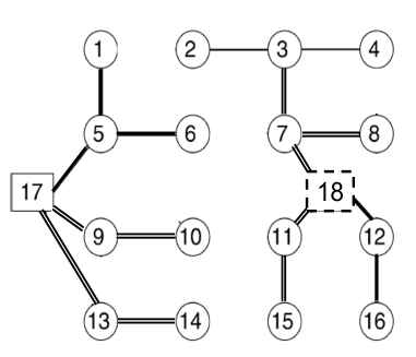
Figure 2: Expansion results with chance of a) 100% and b) 80%

V Conclusion

In this paper, a stochastic second order mixed integer model was constructed and studied for distribution system expansion planning. A chance-constrained variant of the problem was also developed, which can be used to obtain a cost-effective plan by avoiding extreme scenarios. To solve the problem, we developed a novel bilinear Bender decomposition algorithm that handles the conic power flow formulations and deals a chance constraint imposed on stochastic scenarios. On a set of instances, we performed numerical experiments, analyzed our model’s performance and generalized insights.

Based on our numerical experiments, it was demonstrated that our proposed algorithms have a remarkable strength, which drastically outperforms professional mixed integer conic solver CPLEX by orders of magnitude. They therefore greatly improves our solution capacity for this type of problems. Indeed, to the best of our knowledge, it is the first time that chance-constrained stochastic mixed integer SOCP model can be solved efficiently. Because the developed algorithms are generic, we believe that they can be used in other application areas, such as power system expansion and operation planning.

References

- [1] K Tomsovic M Vaziri and A Bose. A direct graph formulation of the multistage distribution expansion problem. Power Delivery, IEEE Transactions on, 19(3):1335–1341, 2004.
- [2] L A Pereira S Haffner, A Pereira and L Barreto. Multistage model for distribution expansion planning with distributed generation— part i: Problem formulation. Power Delivery, IEEE Transactions on, 23(2):915–923, 2008.
- [3] R. Jabr et al. Optimal power flow using an extended conic quadratic formulation. Power Systems, IEEE Transactions on, 23(3):1000–1008, 2008.
- [4] R.Jabr et al. Polyhedral formulations and loop elimination constraints for distribution network expansion planning. Power Systems, IEEE Transactions on, 28(2):1888–1897, 2013.
- [5] J A Taylor and F S Hover. Convex models of distribution system reconfiguration. Power Systems, IEEE Transactions on, 27(3):1407–1413, 2012.
- [6] S Mehrotra C Lee, C Liu and Z Bie. Robust distribution network reconfiguration. Smart Grids, IEEE Transactions on, 6(2):836–842, 2015.
- [7] T. Ding, S. Liu, W. Yuan, Z. Bie, and B. Zeng. A two-stage robust reactive power optimization considering uncertain wind power integration in active distribution networks. Sustainable Energy, IEEE Transactions on, 7(1):301–311, Jan 2016.
- [8] I.J. Ramirez-Rosado and J.A. Dominguez-Navarro. New multiobjective tabu search algorithm for fuzzy optimal planning of power distribution systems. Power Systems, IEEE Transactions on, 21(1):224–233, Feb 2006.
- [9] Kai Zou, A.P. Agalgaonkar, K.M. Muttaqi, and S. Perera. Distribution system planning with incorporating dg reactive capability and system uncertainties. Sustainable Energy, IEEE Transactions on, 3(1):112–123, Jan 2012.
- [10] J. R. Birge and F. Louveaux. Introduction to stochastic programming. Springer Science & Business Media, 2011.
- [11] A. Shabbir and A. Shapiro. Solving chance-constrained stochastic programs via sampling and integer programming. Tutorials in Operations Research, 10:261–270, 2008.
- [12] S. Takriti, J.R. Birge, and E. Long. A stochastic model for the unit commitment problem. Power Systems, IEEE Transactions on, 11(3):1497–1508, Aug 1996.
- [13] Q. Wang, Y. Guan, and J. Wang. A chance-constrained two-stage stochastic program for unit commitment with uncertain wind power output. Power Systems, IEEE Transactions on, 27(1):206–215, 2012.
- [14] Q. P. Zheng, J. Wang, and A. L. Liu. Stochastic optimization for unit commitment: A review. Power Systems, IEEE Transactions on, 30(4):1913–1924, July 2015.
- [15] E. Gil, I. Aravena, and R. Cardenas. Generation capacity expansion planning under hydro uncertainty using stochastic mixed integer programming and scenario reduction. Power Systems, IEEE Transactions on, 30(4):1838–1847, July 2015.
- [16] P. Parpas and M. Webster. A stochastic multiscale model for electricity generation capacity expansion. European Journal of Operational Research, 232(2):359–374, 2014.
- [17] K. Baker, G. Hug, and X. Li. Optimal storage sizing using two-stage stochastic optimization for intra-hourly dispatch. In North American Power Symposium (NAPS), 2014, pages 1–6. IEEE, 2014.
- [18] L. Kuznia, B. Zeng, G. Centeno, and Zh. Miao. Stochastic optimization for power system configuration with renewable energy in remote areas. Annals of Operations Research, 210(1):411–432, 2013.
- [19] K. J. Cormican. Computational methods for deterministic and stochastic network interdiction problems. PhD thesis, Monterey, California. Naval Postgraduate School, 1995.
- [20] U. Janjarassuk and J. Linderoth. Reformulation and sampling to solve a stochastic network interdiction problem. Networks, 52(3):120–132, 2008.
- [21] Jacques F Benders. Partitioning procedures for solving mixed-variables programming problems. Numerische mathematik, 4(1):238–252, 1962.
- [22] R. M V. Slyke and R. Wets. L-shaped linear programs with applications to optimal control and stochastic programming. SIAM Journal on Applied Mathematics, 17(4):638–663, 1969.
- [23] M Shahidehopour and Yong Fu. Benders decomposition: applying benders decomposition to power systems. Power and Energy Magazine, IEEE, 3(2):20–21, 2005.
- [24] S Ganguly, NC Sahoo, and D Das. Recent advances on power distribution system planning: a state-of-the-art survey. Energy Systems, 4(2):165–193, 2013.
- [25] E.G. Carrano, F.G. Guimaraes, R.H.C. Takahashi, O.M. Neto, and F. Campelo. Electric distribution network expansion under load-evolution uncertainty using an immune system inspired algorithm. Power Systems, IEEE Transactions on, 22(2):851–861, May 2007.
- [26] W. Zhou and A. M. Montaz. Generalized benders decomposition for one class of minlps with vector conic constraint. SIAM Journal on Optimization, 25(3):1809–1825, 2015.
- [27] B. Zeng, y. An, and L. Kuznia. Chance constrained mixed integer program: Bilinear and linear formulations, and benders decomposition. Optimization Online, 2014.
- [28] A Ben-Tal and A Nemirovski. Lectures on modern convex optimization: Analysis, algorithms, and engineering applications. MPS/SIAM Series on Optimization, 2015.
- [29] D M Gay R Fourer and B W Kernighan. AMPL: A Modeling Lan-guage for Mathematical Programming. Duxbury Press, 2002.
- [30] K Bhattacharya S Wong and J D Fuller. Electric power distribution system design and planning in a deregulated environment. IET Generation, Transmission & Distribution, 3(12):1061–1078, 2009.
- [31] H B Gooi M Wang S X Chen, Y S Eddy and S F Lu. A centralized reactive power compensation system for lv distribution networks. Power Systems, IEEE Transactions on, 30(1):274–284, 2015.
- [32] L A Pereira S Haffner, A Pereira and L Barreto. Multistage model for distribution expansion planning with distributed generation— part ii: Numerical results. Power Delivery, IEEE Transactions on, 23(2):924–929, 2008.