Complexity-Aware Assignment of Latent Values in Discriminative Models for Accurate
Gesture Recognition

Abstract

Many of the state-of-the-art algorithms for gesture recognition are based on Conditional Random Fields (CRFs). Successful approaches, such as the Latent-Dynamic CRFs, extend the CRF by incorporating latent variables, whose values are mapped to the values of the labels. In this paper we propose a novel methodology to set the latent values according to the gesture complexity. We use an heuristic that iterates through the samples associated with each label value, estimating their complexity. We then use it to assign the latent values to the label values. We evaluate our method on the task of recognizing human gestures from video streams. The experiments were performed in binary datasets, generated by grouping different labels. Our results demonstrate that our approach outperforms the arbitrary one in many cases, increasing the accuracy by up to 10%.

I Introduction

The fields of Computer Vision, Pattern Recognition and Human-Computer Interaction still face the challenging problems of gesture and activity recognition. Over the last two decades, generative models struggled to tackle these problems, and, eventually, with advancements in the inference methods for graphical models, Conditional Random Fields (CRFs) [1] rose as a powerful discriminative alternative for dealing with them, relaxing the dependency assumptions on the inputs.

More recently, models based on CRFs have achieved the state-of-the-art results for such tasks [2, 3, 4]. They are part of a bigger class of models which incorporate latent variables to the original CRF, increasing the model’s expressiveness and its capacity to find relevant substructure in the gestures and activities [5, 6, 2, 3]. Two representative works of this approach are the Latent-Dynamic Conditional Random Fields (LDCRF) [6] and the Multi-View Latent-Dynamic Conditional Random Fields (MV-LDCRF) [2], where there is a direct mapping between the values of the latent variables and the label variables. In other words, there is a disjoint set of latent variable values associated with each label variable value , as it can be seen in Figure 1.

Although these methods improve the original CRF by training the latent variables as if they were the label variables, they add a new parameter that needs to be tuned: the number of latent values associated with each specific label value. In this scenario, two questions arise: i) how the assignment of these numbers impact the accuracy of the model, and if so, ii) how to systematically determine them.

Each latent value may be interpreted as a subset or a sub stage in a gesture or an activity. i.e. In the activity playing a sport, using latent variables we may be able to model the difference between playing football and playing chess, which have a different set of gestures involved [3]. In a composite gesture, such as first raising the right hand, and then the left, we can use latent variables to model both stages differently, as well as their interaction [6]. In this context, the assignment of the number of latent values plays a key role in the development of a model capable of representing the complexity of a gesture or an activity.

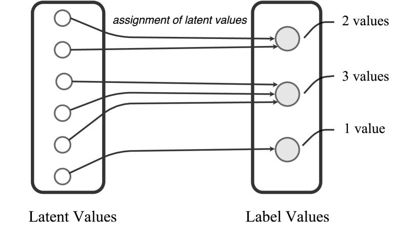
Figure 1: Assignment of the latent values to the label values. The arrows show that each latent value maps into exactly one label value. We improve the existing models by determining this assignment according to the complexity of the gestures.

In this paper we propose an euclidean distance-based algorithm that, given the number of available latent values, determines their assignment among the labels. Our approach inspects the samples associated with each label in order to get an associated complexity measurement, and then uses it to distribute the latent values. We evaluate our method on the task of recognizing human gestures from unsegmented video streams in binary datasets using a LDCRF. Our results show that the distribution of latent values has a high and non-trivial impact on the accuracy of the model, and that using our method improves the performance by up to $10\%$ in accuracy in the tested datasets. The code of our method is available online.

II Related Work

Many different probabilistic graphical models have been used for recognizing human gestures and activities, such as: Hidden Markov Models (HMMs) [7, 8, 9], Dynamic Bayesian Networks (DBNs) [10], and Conditional Random Fields (CRFs) [11, 3]. These graphical models are either generative or discriminative, depending on whether they make independence assumptions on the input or not. As we usually rely on input that is heavily correlated, discriminative models tend to perform better [12], especially for sequence labeling tasks [3, 6]. Sminchisescu et al., for instance, outperformed a HMM approach using a CRF for the task of classifying human motion activities, such as walking and jumping [11].

In several approaches, there is an additional layer of latent variables, which are not observed, but inferred. This layer helps to model complex labels [3, 6, 5, 13, 2] and is also used to exploit the underlying semantics between temporal segments [3]. Although the authors agree with the gains of using a layer of latent variables, they have diverging interpretations on how exactly they do so. Hu et al. stated that latent variables represent a subset of a given label. For instance, take an hypothetical class for the activity to open something. The layer of latent variables would help to model the difference between opening a door and opening a bottle [3]. On the other hand, Morency et al. claim that latent variables represent different stages of a same label being performed [6]. In a complex gesture or activity, different parts of the motion would have different label values, for example.

CRFs are discriminative models which were first introduced by Lafferty et al., and quickly adopted in the vision community [1]. The two most successful extensions for gesture and activity recognition based on CRFs are the Hidden Conditional Random Fields (HCRFs) and the Latent-Dynamic Conditional Random Fields (LDCRFs). The HCRFs add a layer of latent variables that are connected to a single label variable, which predicts the gesture or the activity which was performed for all the observations [5]. The model presented by Hu et al. exploits, by using a HCRF-like structure, full connectivity between input, latent and label variables. The layer of latent variables added has a direct mapping to the label variables. The LDCRFs models, beyond adding the layer of latent variables, have disjoint sets of latent values associated with each label value. They also include one label variable per observation, enabling the output to be a continuous stream, and outperforming models based on Support Vector Machines (SVMs), HMMs, CRFs and HCRFs [6]. A representative LDCRFs approach is presented by Song et al. [2]. They proposed a multi-view version of the LDCRFs and also of the HCRFs. By splitting semantically related input variables in different views, the performance of these models was improved.

Hu et al. and Sung et al. also presented two-layered discriminative models for activity recognition. The model presented by Hu et al. recognizes sub-level activities and high-level activities successively, using the assumption that a high-level activity is composed of multiple sub-activities. While the first layer of the hierarchical model predicts low-level activity for each temporal segment, the second uses the sub-activity to estimate the high-level activity [13]. They added a set of latent variables to enrich the expressiveness of the second layer, and use the sub-activity as an observed variable. The model presented by Sung et al. learns the sub-activities implicitly, by considering them as latent variables [14].

In the aforementioned sequential discriminative models where the latent values have a direct mapping to the label, the assignment of the number of latent values per label value is chosen arbitrarily. Typically the same number of latent values is given for all label values [2, 3, 6]. Our work proposes a systematic way to distribute these, presenting significant performance gains in the tested datasets. Our method is valid for all the models of this category, but we mainly build upon the LDCRFs proposed by Morency et al. [6], since they were used to measure the performance improvements achieved by adopting our approach.

III Methodology

III-A Theoretical Background

In this section we briefly describe the main characteristics and modeling of Conditional Random Fields (CRFs) and Latent Dynamic Conditional Random Fields (LDCRFs). For details on how the inference or the parameter learning can be used, the reader is referred to [15, 16].

III-A1 Conditional Random Fields

We review Conditional Random Fields as presented by Lafferty et al.  [1], but using a factor graph notation for the sake of simplicity.

Let $\mathbf{X}=(X_{1},\ldots,X_{k})$ be a set of observed random variables (e.g. feature vectors such as skeleton joints), and $\mathbf{Y}=(Y_{1},\ldots,Y_{l})$ a set of target random variables (labels). $G$ is a factor graph $(V,E,A)$, whose nodes $V$ have a direct mapping with $\mathbf{X}\cup\mathbf{Y}$, and where $A$ is the set of factors associated with the edges $E$ that map the subset $\mathbf{X_{a}}\cup\mathbf{Y_{a}}$ into a positive real value:

$$A=\{\psi_{1},...,\psi_{m}\},\psi_{a}:\mathbf{Y_{a}}\cup\mathbf{X_{a}}\mapsto\mathbb{R}^{+}.$$ (1)

The graph $G$ is a Conditional Random Field if $P(\mathbf{y}|\mathbf{x})$ factorizes according to Equation 2:

$$P(\mathbf{y}|\mathbf{x})=\frac{1}{Z(\mathbf{x})}\prod_{a\in A}\psi_{a}(\mathbf{y_{a}},\mathbf{x_{a}}),$$ (2)

$$Z(\mathbf{x})=\sum_{\mathbf{y}\in\mathbf{Y}}\prod_{a\in A}\psi_{a}(\mathbf{y_{a}},\mathbf{x_{a}}).$$ (3)

where $Z(\mathbf{x})$ is the partition function. Lower case bold letters represent assignments to these sets of random variables, and $\mathbf{y_{a}}$ and $\mathbf{x_{a}}$ represent the values that correspond to the domain of the factor $\psi_{a}$.

III-A2 Linear Chain Conditional Random Fields

Given the CRF model, is easy to derive a Linear Chain Conditional Random Field, which can be seen in Figure 2. For each edge $(i,j)$ in the chain, define a feature function:

$$f_{k}(v_{i},v_{j})=\begin{cases}1&\text{$(v_{i},v_{j})\in E$}\\ 0&\text{otherwise}\end{cases}.$$ (4)

Let $\log\psi_{a}$ be linear over the set of feature functions $K=\{f_{1},...,f_{m}\}$, and the vector of parameters of the model $\hat{\theta}=\{\theta_{1},...,\theta_{m}\}$:

$$\psi_{a}(\mathbf{y_{a}},\mathbf{x_{a}})=\exp\Bigg{\{}\theta_{a}f_{a}(\mathbf{y_{a}},\mathbf{x_{a}})\Bigg{\}}.$$ (5)

We can then write the Linear Chain CRF as:

$$P(\mathbf{y}|\mathbf{x})=\frac{1}{Z(\mathbf{x})}\exp\Bigg{\{}\sum_{t=1}^{T}\sum_{k=1}^{K}\theta_{k}f_{k}(y_{t},y_{t-1},\mathbf{x_{t}})\Bigg{\}}.$$ (6)

Notice that we iterate through all the $T$ levels of the chain and all the $K$ feature functions. We also modified the notation for feature functions so that they can represent the feature functions of both $label-label$ and $feature-label$ edges at once. The partition function $Z(\mathbf{x})$ is defined as:

$$Z(\mathbf{X})=\sum_{{y_{t},y_{t-1}}\in\mathbf{Y}}\exp\Bigg{\{}\sum_{t=1}^{T}\sum_{k=1}^{K}\theta_{k}f_{k}(y_{t},y_{t-1},\mathbf{x_{t}})\Bigg{\}}.$$ (7)

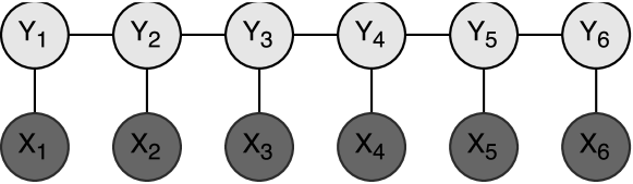
Figure 2: A CRF graphical model. The feature variables $X_{i}$ are connected directly to the label variables $Y_{i}$.

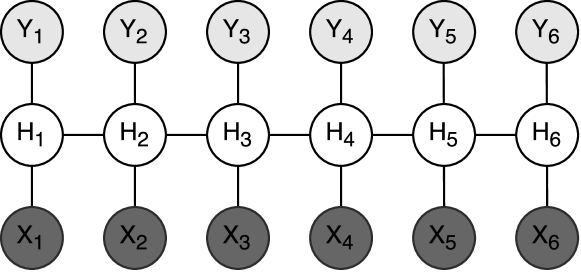
Figure 3: A LDCRF graphical model. A new layer, composed of latent variables $H_{i}$, is used to enrich the expressiveness of the model. The latent variables connect the label variables $Y_{i}$ to the feature variables $X_{i}$ and model the substructure of the gesture or activity.

III-A3 Latent-Dynamic Conditional Random Fields

Another extension for CRF models presented by Morency et al. [6] includes a third set of random variables $\mathbf{H}=(H_{1},\ldots,H_{n})$. The values of variables $H_{i}$ have a direct mapping with the label values, and the probability of each label value a label variable $Y$ might assume is the sum of the probabilities of its associated latent values:

$$P(\mathbf{y}|\mathbf{x})=\sum_{\mathbf{\textbf{h}:\forall h_{j}\in\mathbf{H}_{Y_{j}}}}P(\textbf{h}|\textbf{x}),$$ (8)

where each $h_{j}\in\mathbf{H}_{Y_{j}}$ is a member of the set of possible latent values for the class $Y_{j}$. The final probability distribution $P(\textbf{h}|\textbf{x})$ considering the latent variables instead of the label ones is given by:

$$P(\mathbf{h}|\mathbf{x})=\frac{1}{Z(\mathbf{x})}\exp\Bigg{\{}\sum_{t=1}^{T}\sum_{k=1}^{K}\theta_{k}f_{k}(h_{t},h_{t-1},\mathbf{x})\Bigg{\}},$$ (9)

$$Z(\mathbf{x})=\sum_{{h_{t},h_{t-1}}\in\mathbf{H}}\exp\Bigg{\{}\sum_{t=1}^{T}\sum_{k=1}^{K}\theta_{k}f_{k}(h_{t},h_{t-1},\mathbf{x})\Bigg{\}}.$$ (10)

A graphical representation of a LDCRF model is depicted in Figure 3.

III-B The Semantics of Latent Values

As stated, in a Latent Dynamic Conditional Random Field, we split each target variable value $y_{t}$ into a series of equivalent latent values $\mathbf{h}$. This increases the capacity of the model to represent complex labels, because it allows us to train a classifier to a larger number of labels than the existing ones [6].

Consider, for instance, an LDCRF that receives the positions of the joints of individuals as an input and has to decide which sports people are playing at each frame. There are a myriad of sports with distinct gestures and actions involved, and, therefore, one could divide a class $sport$ into other simpler, more atomic classes, such as $(football,handball,chess)$. This is, intuitively, how Hu et al. view the role of latent values [3]. They allow different subsets of an activity or gesture to be represented by different label values, which improves the accuracy.

Another perspective is provided by Morency et al., which view the role of the latent variables as a way to model the sub stages of a given gesture or activity [6]. Let’s consider a gesture with a complex substructure, such as a sequence of signals in American Sign Language (ASL). In this case, different latent values may model different parts of the gesture. Differently from Hu’s perspective, the idea is that the same gesture may be modeled by different latent values in different stages of the gesture.

In the following sections, we describe our algorithm for assigning the number of latent values per class that takes those insights into consideration. Figures 4 and 5 illustrate the feature space of a CRF and of a LDCRF with different sets of latent values for each label, giving further insight on how this assignment is done. In Figure 4 we classify the entries as one of the four labels directly, whereas in Figure 5 we classify them as one of the seven values our latent variable might assume and then map those values into the label values.

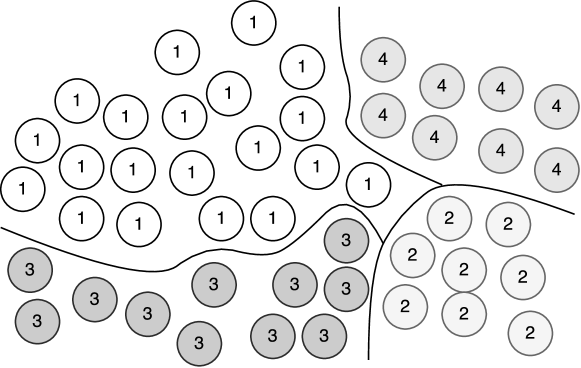
Figure 4: Feature space of a CRF model. The lines separate the instances assigned to different label values.

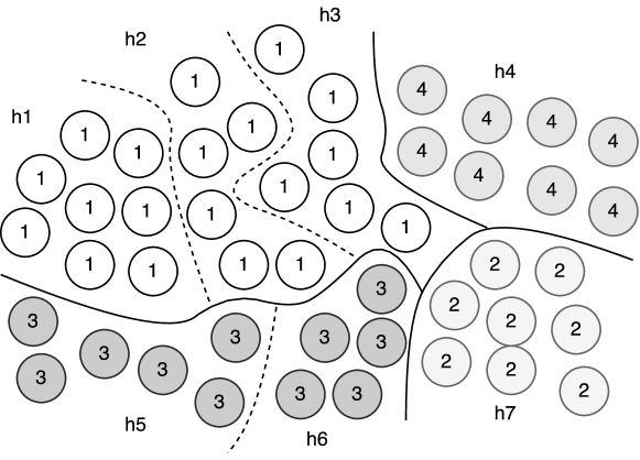
Figure 5: Feature space of a latent model. Notice that we have $\mathbf{H}_{Y_{1}}=\{h_{1},h_{2},h_{3}\},\mathbf{H}_{Y_{2}}=\{h_{7}\},\mathbf{H}_{Y_{3}}=\{h_{5},h_{6}\},\mathbf{H}_{Y_{4}}=\{h4\}$. The dashed lines separate the instances assigned to different latent values.

III-C Computing The Complexities and Assigning Latent Values

In order to decide which of the label values will benefit from having multiple latent values assigned to it, we propose a heuristic algorithm for finding the labels which can be better represented by many subsets or substages and the proportion to which they should receive latent values.

In the first step, we compute a measure of the complexity associated with each of the labels of the classifier according to Algorithm 1. Let $\mathcal{L}=\{l_{1},l_{2},l_{3}...,l_{n}\}$ be a set of labels in a dataset. We normalize the different samples that have the same label values  (lines $2$ – $8$) and then calculate the point-to-point euclidean distance between the pairs of features of these samples (lines $11$ – $17$). This measures the complexities associated with each label, $v_{0},\ldots,v_{n}$, by estimating the difference among the samples of a given label. Each complexity measurement $v_{i}$ is then normalized, dividing it by the total sum of all measurements (lines $18$ – $21$). This makes $v_{i}\in[0,1]$ and $\sum_{\forall i\in Y}v_{i}=1$.

This heuristic is in agreement with the intuitions previously presented. If there are labels with different sub activities or sub gestures, as one would obtain from grouping opening a bottle and opening a door in the same label, when we calculate the point-to-point euclidean distance between the pairs of features, we would get a high value, as the samples from different sub activities will differ among themselves. Consequently, we then assign more latent values to these labels.

On the other hand, if we have labels with a complex substructure, is it expected that there will be an overlap between different stages of the gesture when we take the point-to-point euclidean distance. Indeed, such assumption makes sense, since people will not execute each part of a complex gesture or activity in the exact same time. Notice that considering this setting we also will give a higher measure of complexity for labels with several sub stages.

Once we computed the complexities, we proceed to distribute the latent values according to Algorithm 2. Our algorithm increments the number of latent values associated with a given label value such that the normalized array $norm$ will be close to the array $v$ calculated in the first algorithm (lines $5$ – $11$). The algorithm receives as input the number of values we want to distribute, the complexity measures calculated in the previous step, the set of distinct labels and a real value $c\in[0,1]$. Notice that $c$ is a limit for the maximum percentage of latent values that one label value might claim. In the array $buckets=\{v_{1},...,v_{n}\}$, the position $buckets[i]$ is the number of latent values assigned to the i-th label.

IV Experiments

We evaluated our method on the task of unsegmented human gesture recognition using binary datasets. Those were created by grouping the labels of existing datasets such as the ArmGesture dataset and a subset of $6$ labels of the NATOPS dataset. Bellow we describe them, give details of our implementation and on the experiments protocol.

IV-A Datasets

The ArmGesture dataset [17] contains the data on six arm gestures described by 2D joint angles and 3D euclidean coordinates for left/right shoulders and elbow. The six gestures are presented in Figure 6 (a). The data was collected from $13$ participants with an average of $120$ samples per class, and subsampled by the factor of $2$ [2].

The NATOPS dataset [18] contains twenty-four body/hand gestures used when handling aircraft on the deck of an aircraft carrier. We used the same subset of gestures chosen by Song et al. [2]. These gestures can be seen in Figure 6 (b).

One of drawbacks of these datasets is that the gestures do not differ much in terms of complexity. Thus, in order to better measure the impact of our method, we generate datasets were different labels have different complexity measurements, but that are still based on real world data. Given the two original datasets, we make them binary by grouping the labels into two sets, each of which will become a new label. Notice that there are several grouping strategies. For instance, in a dataset with labels $(\{l_{1}\},\{l_{2}\},\{l_{3}\}...\{l_{n}\})$, one may group the label as $(\{l_{1}\},\{l_{2},l_{3}...l_{n}\})$, $(\{l_{1},l_{2}\},\{l_{3}...l_{n}\})$.

Since we also want to evaluate how our model performs when the samples contain several gestures, we created new versions by grouping the different video segments of the original datasets in groups of three and concatenate them. We call these datasets many gestures datasets, and the other ones single gesture datasets.

Each created dataset is identified by the following expression:

$$concat(id,\{1st\_labels\_set\},-,\{2nd\_labels\_set\}),$$

where $id$ is either AG for the ArmGesture dataset or NT for the NATOPS dataset, the label fields are the numbers of the labels grouped together (separated by an hyphen). The expression NT01$-$2345, for instance, refers to the dataset created by grouping the labels $\{0,1\}$ and the labels $\{2,3,4,5\}$ in the NATOPS dataset. We then have to specify if the dataset has many gestures or a single gesture.

1:procedure CompMeasure($instances$, $\mathcal{L}$)

2:     for $l\in\mathcal{L}$ do

3:         $aux\leftarrow$ instances of label $l$

4:         $length\leftarrow argmax(aux.length)$

5:         for $\forall x\in aux$ do

6:              $x\leftarrow linearInterpolation(x,length)$

7:         end for

8:     end for

9:     $n\leftarrow\mathcal{L}.length$

10:     $v\leftarrow zeros(n)$

11:     for $l\in\mathcal{L}$ do

12:         $aux\leftarrow$ instances of label $l$

13:         for $\forall x,y\in aux$ do

14:              $dist\leftarrow euclideanDistance(x,y)$

15:              $v[l]\leftarrow v[l]+dist$

16:         end for

17:     end for

18:     $valuesSum\leftarrow v[0]+...+v[n]$

19:     for $\forall s\in v$ do

20:         $s\leftarrow s\div valuesSum$

21:     end for

22:     return $v$

23:end procedure

Algorithm 1 Algorithm for measuring the complexity of each label.

1:procedure Dist($number$, $values$, $\mathcal{L}$, $c$)

2:     $n\leftarrow\mathcal{L}.length$

3:     $buckets\leftarrow ones(n)$

4:     $left=number-\mathcal{L}.length$

5:     while $left\neq 0$ do

6:         $norm\leftarrow(b_{i})\div(\sum\limits_{j\in buckets}b_{j}),\forall i\in buckets$

7:         $dif\leftarrow abs(buckets-values)$

8:         $i\leftarrow indexMin(dif)$ s.t. the normalized array where we we add $1$ to $b_{i}$ has $b_{i}<c$.

9:         $left\leftarrow left-1$

10:         $bucket[i]\leftarrow bucket[i]+1$

11:     end while

12:     return $buckets$

13:end procedure

Algorithm 2 Algorithm for distributing latent values across labels values given a complexity measurement.

IV-B Experiments Protocol

We performed three experiments with the datasets. The first one is a proof of concept on how the assignment of latent values may change the accuracy of a LDCRF. The second and the third ones make comparisons between the accuracy of a LDCRF whose states have been assigned using our method and arbitrarily.

IV-B1 Experiment 1

As stated, this experiment is a proof of concept to show that the assignment of the latent values is non-trivial and has a considerable impact in the accuracy.

For a the NT23$-$0145 many gestures dataset we plot the confusion matrix (Figure 7) of four different assignments of latent values. In the first assignment, the first label value has two associated latent values and the second one has only one, whereas in second assignment the first label value has one associated latent value and the second one has two. The remaining assignments are the cases where both labels values have either one and two latent values, respectively. The training and the test sets were obtained by dividing the dataset into three parts, from which $2/3rds$ were for the training and the remaining $1/3rd$ for testing.

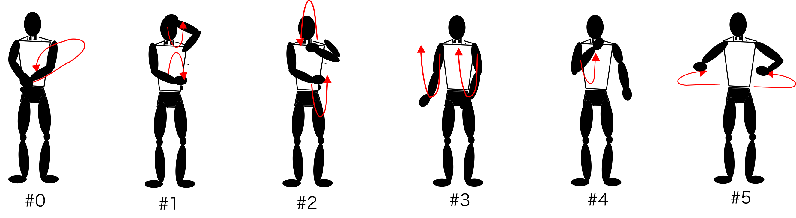
(a) Gestures from the ArmGesture dataset.

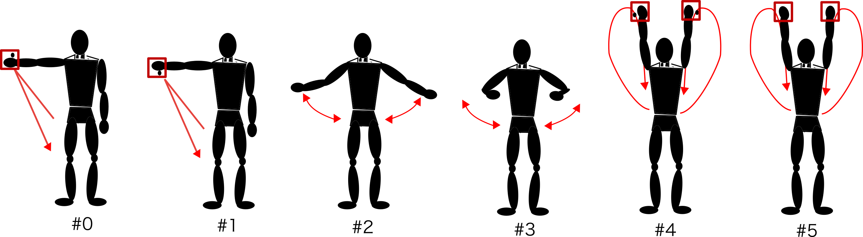
(b) Gestures from the NATOPS dataset.

Figure 6: Datasets used in experiments.

TABLE I: Results of our method in binary datasets. We present the accuracy and the standard deviation for two values of $c$ and the normal distribution. We also present the percentage of the complexity values calculated for each of the two binary labels in row CM.

		Single Gesture				Many Gestures
Exp	Dataset	Ours c=1	Ours c=0.75	Normal	CM	Ours c=1	Ours c=0.75	Normal	CM
	AG0$-$12345	$98.9\pm 0.3$	$97.2\pm 3.3$	$98.9\pm 0.3$	$02,98$	$97.3\pm 1.3$	$97.5\pm 0.9$	$97.7\pm 1.1$	$03,97$
	AG01$-$2345	$99.2\pm 0.4$	$99.3\pm 0.5$	$99.2\pm 0.4$	$14,86$	$85.0\pm 24.8$	$97.2\pm 0.8$	$97.3\pm 1.3$	$14,86$
	AG012$-$345	$94.3\pm 0.4$	$93.8\pm 0.9$	$94.3\pm 0.4$	$41,59$	$89.2\pm 2.9$	$90.7\pm 0.6$	$90.6\pm 0.9$	$37,63$
	NT0$-$12345	$92.7\pm 0.9$	$92.8\pm 1.0$	$92.9\pm 1.2$	$02,98$	$91.5\pm 1.2$	$92.6\pm 0.8$	$92.0\pm 1.1$	$03,97$
	NT01$-$2345	$92.2\pm 1.6$	$\mathbf{96.3\pm 1.0}$	$86.6\pm 13.4$	$13,87$	$86.2\pm 3.6$	$\mathbf{93.8\pm 0.4}$	$83.8\pm 22.0$	$17,83$
II	NT012$-$345	$79.5\pm 12.6$	$73.4\pm 12.6$	$79.5\pm 12.6$	$45,55$	$74.2\pm 1.3$	$\mathbf{79.5\pm 17.6}$	$74.2\pm 1.3$	$52,48$
	AG01$-$2345	$99.2\pm 0.4$	$99.3\pm 0.5$	$99.2\pm 0.4$	$14,86$	$85.0\pm 24.8$	$97.2\pm 0.8$	$97.3\pm 1.3$	$14,86$
	AG12$-$0345	$95.6\pm 1.0$	$95.4\pm 0.7$	$95.4\pm 0.7$	$18,82$	$90.1\pm 1.6$	$90.4\pm 1.3$	$90.5\pm 1.9$	$14,86$
	AG23$-$0145	$99.8\pm 0.3$	$99.8\pm 0.3$	$99.8\pm 0.3$	$18,82$	$96.9\pm 1.7$	$\mathbf{97.2\pm 1.1}$	$94.7\pm 4.8$	$19,81$
	AG34$-$0125	$96.1\pm 1.3$	$96.1\pm 1.3$	$96.1\pm 1.3$	$32,68$	$90.8\pm 1.6$	$90.8\pm 1.6$	$90.8\pm 1.6$	$38,62$
	AG45$-$0123	$98.2\pm 1.0$	$98.2\pm 1.0$	$98.2\pm 1.0$	$22,78$	$\mathbf{96.3\pm 1.2}$	$95.4\pm 0.7$	$94.6\pm 0.3$	$27,73$
	NT01$-$2345	$92.2\pm 1.6$	$\mathbf{96.3\pm 1.0}$	$86.6\pm 13.4$	$13,87$	$86.2\pm 3.6$	$\mathbf{93.8\pm 0.4}$	$83.8\pm 22.0$	$17,83$
	NT12$-$0345	$71.9\pm 3.1$	$71.8\pm 1.1$	$\mathbf{73.4\pm 1.7}$	$19,81$	$70.5\pm 1.6$	$72.4\pm 3.4$	$72.0\pm 2.3$	$23,77$
	NT23$-$0145	$\mathbf{92.2\pm 1.7}$	$84.0\pm 0.9$	$86.2\pm 5.1$	$24,76$	$\mathbf{89.7\pm 1.8}$	$81.1\pm 1.4$	$85.7\pm 12.0$	$23,77$
	NT34$-$0125	$69.6\pm 0.9$	$69.8\pm 1.0$	$70.0\pm 1.4$	$22,78$	$69.3\pm 1.6$	$\mathbf{69.7\pm 1.6}$	$66.8\pm 1.8$	$20,80$
III	NT45$-$0123	$99.3\pm 0.0$	$99.3\pm 0.1$	$99.3\pm 0.1$	$20,80$	$94.4\pm 1.0$	$\mathbf{94.7\pm 1.2}$	$87.8\pm 10.4$	$21,79$

IV-B2 Experiment 2 and 3

For Experiments 2 and 3, we compare the accuracy of training a LDCRF with our method of assigning latent values (for two values of $c$, $0.75$ and $1$) with the accuracy of an arbitrary assignment. We split the data into a test set of $1/3rd$ of the data, and performed a 5-fold cross validation in the remaining $2/3rds$. We then obtain total number of latent values to which had the best performance in the 5-fold cross validation for our method of assignment and for the arbitrary one. This parameters is then used to train the model with what was the validation $2/3rds$ of the data and test it with the $1/3rd$ which was originally the test set. This procedure is repeated $3$ times, varying the validation set chosen initially (as in a 5-fold cross validation nested inside a 3-fold cross validation).

In the validation phase, we selected the total number of latent variable values from a predetermined number of possibilities. For the binary datasets created from the ArmGesture dataset those values were $\{2,4,6,8,10,12,14\}$ and for the datasets created from the NATOPS dataset those values were $\{2,4,6,8\}$. The choice of these values adopted three criteria: (i) even numbers, so that the arbitrary assignment always gave all labels the same amount of latent values, (ii) feasibility for computing time, (iii) values that do not over-fit the model.

In Experiment 2 we created the datasets using the following algorithm: we start with the label grouping $\{\},\{l_{0},l_{1},l_{2},l_{3},l_{4},l_{5}\}$. Then we incrementally create new datasets by adding the label with the lowest index from the second group to the first group and generating the correspondent binary dataset. We stop when both groups have the same number of labels. The idea behind exploring this pattern is to see how the difference in the complexity of binary labels would affect the method. Notice that this is possible because as we add more label values to be collapsed in the first of the mentioned groups, we decrease the difference of the complexity measurement between the two label values.

In Experiment 3 we created the datasets by combining the labels in all possible forms to obtain two groups, containing two and three labels respectively. These labels are then collapsed to generate the binary labels of the new dataset. We explore this pattern to see how our assignment would improve the LDCRF given a more subtle difference in the complexity measurement of the binary label values.

IV-C Implementation Details

We implemented our Latent Dynamic CRF based on the Latent Graph CRF model from PyStruct [19]. For the inference we use the Quadratic Pseudo-Boolean Optimization (QPBO), with the interface also provided by PyStruct. The initial assignment of the latent values was done with a deterministic implementation of the k-means clustering technique, which uses a PCA to initialize its centroids.

V Results

In this section we present and analyze the results of the experiments proposed in Section IV.

V-A Experiment 1

The confusion matrix of the assignment of latent values, $(1,2),(2,1),(1,1),(2,2)$  for the NT23$-$0145 dataset, can be seen in Figure 7. Each row of each matrix is normalized so that we can compare the gains of a given latent value assignment for each of the classes. The results show that the model with the $(2,1)$ assignment has the better accuracy trade-off, with approximately $89.5\%$ average accuracy . It is worth mentioning that the model with the $(2,2)$ assignment is significantly worse than all the others, with only $51.5\%$ average accuracy. A clear example of a case where more latent values do not correspond to a better model. Together, these results show that assigning the latent values according to our computed complexity measurement improves the accuracy of the LDCRF. Additionally, they show that this assignment has a non-trivial impact in the accuracy of the model.

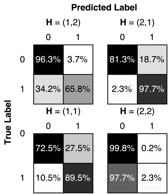
Figure 7: Confusion matrix for the NT23$-$0145 many gestures dataset using different assignments of latent values. The rows of the matrix are normalized, for comparing the accuracy of the classes and the shading of each cell is proportional to the number of instances that correspond to the given scenario.

V-B Experiment 2 and 3

The results for Experiments 2 and 3 are shown in Table I. We present results for our approach for two values of $c$ and also for the arbitrary assignment. The column CM contains the calculated complexity measurement for the two labels in the dataset. The cells in bold indicate cases where the accuracy achieved by training the model with our method was $1\%$ bigger than the arbitrary choice, as well as cases where the arbitrary choice outperformed ours by $1\%$. Notice that the second scenario happened once, in the NT12$-$0345 dataset, where the arbitrary assignment had an accuracy slightly higher than ours. On the other hand, our method outperformed the arbitrary choice by significant values in the many cases. In the NT01$-$2345 single gesture dataset and in the NT01$-$2345 many gestures datasets, for instance, we increased the accuracy of the method by roughly $10\%$.

Two interesting questions that might arise given the results shown are (i) why does our method gives much better results with the NATOPS dataset than with the ArmGesture dataset and (ii) why does our method performs better in datasets where the difference in the estimated complexity for the binary labels is not too big. We draw the following observations. The low gains in performance in the ArmGesture dataset is probably due to how easy the dataset is. The accuracy is already too high with modeling that uses just a few latent values, and adding more models just makes the dataset overfit. In many cases the models selected in the validation for the ArmGesture dataset used only two latent values, which is equivalent to a normal linear chain CRF. It is worth noting that, when we have a larger imbalance in the complexity of the binary labels, it also becomes easier to classify, as one must only learn less complex labels. This might be the reason of the better performance of our method compared to the arbitrary assignment in datasets whose difference in the associated complexity of the binary label is small.

VI Conclusion

The assignment values of latent values is an important parameter in CRF based models with a layer of latent variables. The previous work on such models had a very intuitive approach towards the purpose of the latent variables, and did not address the problem of finding an ideal assignment of these values throughout the label values.

We introduced a new method for assigning them in Latent-Dynamic Conditional Random Fields which outperforms an arbitrary distribution of those values. We evaluated our approach using real world binary datasets for the task of unsegmented human gesture recognition, and provided empirical results of the advantages of our method. The method is generalizable for all the models with a latent layer whose values have a direct mapping with the label values.

Our method showed significant improvements in the hardest of the datasets we used for benchmarking (the NATOPs dataset), and was particularly effective when the difference in the complexity measurement calculated was not too high. By applying our technique we increased the recognition accuracy by roughly $10\%$ in some cases.

In the future, it is of interest to investigate the semantics of the latent layer and its impact on the models performance. To help in such investigation, we plan to create a new dataset where the labels have a significant difference with respect to complexity.

References

- [1] J. Lafferty, A. McCallum, and F. C. Pereira, “Conditional random fields: Probabilistic models for segmenting and labeling sequence data,” 2001.
- [2] Y. Song, L.-P. Morency, and R. Davis, “Multi-view latent variable discriminative models for action recognition,” in Computer Vision and Pattern Recognition (CVPR), 2012 IEEE Conference on. IEEE, 2012, pp. 2120–2127.
- [3] N. Hu, G. Englebienne, Z. Lou, and B. Krose, “Learning latent structure for activity recognition,” in Robotics and Automation (ICRA), 2014 IEEE International Conference on. IEEE, 2014, pp. 1048–1053.
- [4] C. M. de Souza Vicente, E. R. Nascimento, L. E. C. Emery, C. A. G. Flor, T. Vieira, and L. B. Oliveira, “High performance moves recognition and sequence segmentation based on key poses filtering,” in 2016 IEEE Winter Conference on Applications of Computer Vision (WACV), March 2016, pp. 1–8.
- [5] S. B. Wang, A. Quattoni, L. Morency, D. Demirdjian, and T. Darrell, “Hidden conditional random fields for gesture recognition,” in Computer Vision and Pattern Recognition, 2006 IEEE Computer Society Conference on, vol. 2, 2006, pp. 1521–1527.
- [6] L. Morency, A. Quattoni, and T. Darrell, “Latent-dynamic discriminative models for continuous gesture recognition,” in Computer Vision and Pattern Recognition, 2007. CVPR ’07. IEEE Conference on, June 2007, pp. 1–8.
- [7] S. Fujie, Y. Ejiri, K. Nakajima, Y. Matsusaka, and T. Kobayashi, “A conversation robot using head gesture recognition as para-linguistic information,” in Robot and Human Interactive Communication, 2004. ROMAN 2004. 13th IEEE International Workshop on. IEEE, 2004, pp. 159–164.
- [8] M. Assan and K. Grobel, “Video-based sign language recognition using hidden markov models,” in Gesture and Sign Language in Human-Computer Interaction. Springer, 1997, pp. 97–109.
- [9] J. Sung, C. Ponce, B. Selman, and A. Saxena, “Unstructured human activity detection from rgbd images,” in Robotics and Automation (ICRA), 2012 IEEE International Conference on. IEEE, 2012, pp. 842–849.
- [10] Y.-c. Ho, C.-h. Lu, I.-h. Chen, S.-s. Huang, C.-y. Wang, L.-c. Fu et al., “Active-learning assisted self-reconfigurable activity recognition in a dynamic environment,” in Proceedings of the 2009 IEEE international conference on Robotics and Automation. IEEE Press, 2009, pp. 1567–1572.
- [11] C. Sminchisescu, A. Kanaujia, and D. Metaxas, “Conditional models for contextual human motion recognition,” Computer Vision and Image Understanding, vol. 104, no. 2, pp. 210–220, 2006.
- [12] A. Y. Ng and M. I. Jordan, “On discriminative vs. generative classifiers: A comparison of logistic regression and naive bayes,” in Advances in Neural Information Processing Systems 14, T. G. Dietterich, S. Becker, and Z. Ghahramani, Eds. MIT Press, 2002, pp. 841–848.
- [13] N. Hu, G. Englebienne, and B. Krose, “A two-layered approach to recognize high-level human activities,” in Robot and Human Interactive Communication, 2014 RO-MAN: The 23rd IEEE International Symposium on, Aug 2014, pp. 243–248.
- [14] J. Sung, C. Ponce, B. Selman, and A. Saxena, “Unstructured human activity detection from rgbd images,” in Robotics and Automation (ICRA), 2012 IEEE International Conference on, May 2012, pp. 842–849.
- [15] C. Sutton and A. McCallum, “An introduction to conditional random fields,” Machine Learning, vol. 4, no. 4, pp. 267–373, 2011.
- [16] S. Nowozin and C. H. Lampert, “Structured learning and prediction in computer vision,” Found. Trends. Comput. Graph. Vis., vol. 6, pp. 185–365, Mar. 2011.
- [17] A. Quattoni, S. Wang, L.-P. Morency, M. Collins, and T. Darrell, “Hidden conditional random fields,” IEEE Transactions on Pattern Analysis & Machine Intelligence, no. 10, pp. 1848–1852, 2007.
- [18] Y. Song, D. Demirdjian, and R. Davis, “Tracking body and hands for gesture recognition: Natops aircraft handling signals database,” in Automatic Face & Gesture Recognition and Workshops (FG 2011), 2011 IEEE International Conference on. IEEE, 2011, pp. 500–506.
- [19] A. C. Müller and S. Behnke, “pystruct - learning structured prediction in python,” Journal of Machine Learning Research, vol. 15, pp. 2055–2060, 2014.