A boundary integral equation method for mode elimination and vibration confinement in thin plates with clamped points

Abstract

We consider the bi-Laplacian eigenvalue problem for the modes of vibration of a thin elastic plate with a discrete set of clamped points. A high-order boundary integral equation method is developed for efficient numerical determination of these modes in the presence of multiple localized defects for a wide range of two-dimensional geometries. The defects result in eigenfunctions with a weak singularity that is resolved by decomposing the solution as a superposition of Green’s functions plus a smooth regular part. This method is applied to a variety of regular and irregular domains and two key phenomena are observed. First, careful placement of clamping points can entirely eliminate particular eigenvalues and suggests a strategy for manipulating the vibrational characteristics of rigid bodies so that undesirable frequencies are removed. Second, clamping of the plate can result in partitioning of the domain so that vibrational modes are largely confined to certain spatial regions. This numerical method gives a precision tool for tuning the vibrational characteristics of thin elastic plates.

1 Introduction

The eigenvalues of fourth-order differential operators are central in determining mechanical properties of rigid bodies. This paper considers the small amplitude out-of-plane vibrations of a thin elastic plate [44]. The vibrational frequencies $\lambda>0$ and modes $u(\mathbf{x})$ satisfy the bi-Laplacian eigenvalue problem

$$\Delta^{2}u=\lambda u,\qquad\mathbf{x}\in\Omega;\qquad\int_{\Omega}u^{2}\,d\mathbf{x}=1,$$ (1a)

where $$\Omega\subset\mathbb{R}^{2} \mathbf{x}=(x,y) \Delta^{2}u:=u_{xxxx}+2u_{xxyy}+u_{yyyy} \partial\Omega$$ is a closed planar region representing the extent of the plate, , and . Conditions on the boundary are application specific, with a common condition being that the plate is clamped on its periphery which stipulates that

$$u=\partial_{\mathbf{n}}u=0,\qquad\mathbf{x}\in\partial\Omega,$$ (1b)

where $$\partial_{\mathbf{n}}$$ is the outward facing normal derivative. A wide variety of engineering systems utilize thin perforated plates in their construction. Examples include heat exchangers [41, 47, 35], porous elastic materials, and acoustic tilings [5, 48, 30]. The specific placement of these perforations permits the manipulation of acoustic and vibrational properties of the plate while economizing on weight and material cost. Homogenization theories have been proposed to replace the natural elastic modulus of the plate with an effective modulus [11, 4], however, an averaging approach omits the pronounced localizing effects that clamping has on vibrational modes [23].

Figure 1: In the limit of vanishing hole radius ${\displaystyle\varepsilon}\to 0$, a point constraint $u(\mathbf{x}_{j})=0$ must be enforced at each of the hole centers for $j=1,\ldots,M$.

In the present work, we consider a finite collection of $M$ defects or punctures on (1a) with the conditions

$$u(\mathbf{x}_{j})=0,\qquad j=1,\ldots,M.$$ (1c)

These point constraints arise in singular perturbation studies of (1a) in the presence of $M$ small circular perforations of radius ${\displaystyle\varepsilon}$ (cf. Fig. 1). As the radius ${\displaystyle\varepsilon}$ of the perforations shrink to zero, the behavior of the limiting eigenvalue $\lambda_{{\displaystyle\varepsilon}}$ as ${\displaystyle\varepsilon}\to 0$ satisfies [36, 39, 38, 12]

$$\lambda_{{\displaystyle\varepsilon}}=\lambda+4\pi\nu\sum_{j=1}^{M}|\nabla u(\mathbf{x}_{j})|^{2}+\mathcal{O}(\nu^{2}),\qquad\nu=-\frac{1}{\log{\displaystyle\varepsilon}},$$ (2)

where $(\lambda,u)$ satisfies (1a-1b) plus the point constraints (1c). In the degenerate case $\sum_{j=1}^{M}|\nabla u(\mathbf{x}_{j})|^{2}=0$, equation (2) is not valid and a separate limiting form can be derived [12, 36]. The fact that the clamping condition on each perforation leaves an imprint as the radius shrinks to zero (Fig. 1) implies that no matter how small a perforation is, the vibrational characteristics are distinct from the no hole problem

$$\Delta^{2}u^{\star}=\lambda^{\star}u^{\star},\quad\mathbf{x}\in\Omega;\qquad u^{\ast}=\partial_{\mathbf{n}}u^{\star}=0,\quad\mathbf{x}\in\partial\Omega;\qquad\int_{\Omega}{u^{\star}}^{2}d\mathbf{x}=1.$$ (3)

The discontinuous limiting behavior of (2) is qualitatively different from the spectral problem for the Laplacian in the presence of small perturbing holes [24, 34, 42, 49, 50]. A consequence of the point constraints (1c) is that the eigenfunctions $u(\mathbf{x})$ are not necessarily smooth but satisfy local conditions

$$u(\mathbf{x})=\alpha_{j}|\mathbf{x}-\mathbf{x}_{j}|^{2}\log|\mathbf{x}-\mathbf{x}_{j}|+\mathcal{O}(1),\qquad\mathbf{x}\to\mathbf{x}_{j};\qquad j=1,\ldots,M,$$ (4)

where the constants $\{\alpha_{j}\}_{j=1}^{M}$ reflect the strength of each puncture and depend on the domain $\Omega$ and the clamping locations $\{\mathbf{x}_{j}\}_{j=1}^{M}$. The difference between the punctured eigenvalues $\lambda$ of (1) and the puncture free eigenvalues $\lambda^{\star}$ of (3) satisfies (cf. [38])

$$(\lambda-\lambda^{\star})\braket{u,u^{\star}}=-8\pi\sum_{j=1}^{M}\alpha_{j}u^{\star}(\mathbf{x}_{j}),\qquad\braket{u,u^{\star}}=\int_{\Omega}u(\mathbf{x})u^{\star}(\mathbf{x})\,d\mathbf{x}.$$ (5)

The presence of clamped locations also has a profound localizing effect on the eigenfunctions. In a rectangular domain with a single clamped point located along the long axis, the effect of clamping on (1) has been observed (cf. [23]) to partition $\Omega$ into two distinct domains on the left and right of the clamping location, as shown in Fig 2. One aim of this work is to numerically investigate the global effects that point constraints have on the eigenfunctions of (1) in a variety of different planar geometries.

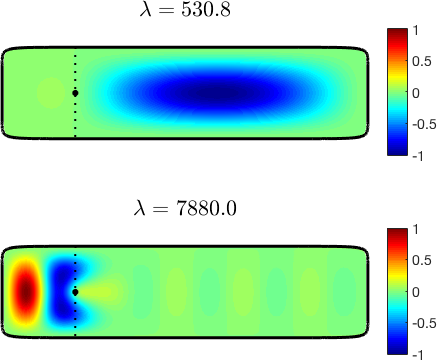
Figure 2: The localization of two eigenfunctions by a single clamped point, located at the black point, in a rectangular domain. In each case, the eigenfunction is essentially zero on one side of the clamping point. See [23] and Sec. 4.2 for more details.

Fourth-order eigenvalue problems (Equations (1) and (3)) exhibit other qualitatively different properties compared to the well-understood Laplacian counterpart. For example, the fundamental eigenfunction of (1), ie. the mode associated with the lowest eigenvalue, is not necessarily single signed [16, 15, 46, 14, 26, 28]. In contrast, the fundamental eigenfunction of the Laplacian is always single signed and the corresponding eigenvalue is simple [21, 27]. An elementary example of this phenomenon is the annular domain ${\displaystyle\varepsilon}<r<1$ in which the radially symmetric and mode $1$ eigenvalues of the bi-Laplacian cross at ${\displaystyle\varepsilon}^{-1}\approx 762.36$ [15]. Correspondingly, for ${\displaystyle\varepsilon}^{-1}>762.36$, the fundamental eigenfunction has multiplicity two and one nodal line. Also, in domains with a corner, the first eigenfunction may possess an infinite number of nodal lines [14]. Many numerical methods have been developed to treat fourth-order eigenvalue problems in view of these characteristics [10, 3, 13, 37, 31, 52].

The main goal of this paper is to introduce a novel high-order boundary integral equation method for the numerical solution of (1) in the presence of a finite collection of punctures (1c). High-order methods for computing eigenvalues of the Laplacian and Helmholtz equations in two and three dimensions have been developed with domain decomposition methods [9, 17, 18], radial basis functions [43], boundary integral equations [6, 45, 20], the method of particular solution [7, 25, 33], the Dirichlet to Neumann map [8], and chebfun [19]. The method of fundamental solutions has also been used to compute eigenvalues of the biharmonic equation [40, 3]. However, none of these works consider the eigenvalue problem with clamped points. We extend the work of one of the previous authors [38] where a finite difference method coupled with an inexact Newton method is used to solve (1) in the unit circle with symmetrically chosen clamped points. Owing to the accuracy and robustness of the boundary integral equation methods, our new method forms third-order solutions of (1) in smooth two-dimensional geometries, including multiply-connected geometries (Figure 13), and with a large assortment of clamping locations.

Using our new method, we demonstrate the dependence of $\lambda$ on the number $M$ and locations $\{\mathbf{x}_{1},\ldots,\mathbf{x}_{M}\}$ of the puncture sites for a variety of planar regions $\Omega\subset\mathbb{R}^{2}$. In particular, we investigate two effects that clamped points have on the vibrational properties of plates with various regular and irregular geometries. Our first observation is that by specific location of punctures, the vibrational properties can be dramatically altered—in particular, undesirable frequencies of vibration can be tuned out by deliberate location of clamped points at nodal lines of the unclamped eigenfunction $u^{\star}$ of (3). Our second observation, extending previous results in [23] for rectangular domains, is that mode confinement occurs in a variety of two dimensional geometries.

The outline of the paper is as follows. In Section 2 we describe the details of a boundary integral method for solving (1). In Section 3, the implementation details are discussed and third-order convergence of the method is verified for a closed-form solution of (1). In Section 4, we apply our method to a disk, rectangles, an ellipse, a non-symmetric shape, and a multiply-connected region. Finally, in Section 5 we discuss the results and areas of future investigations.

2 Integral equation formulation of the clamped eigenvalue problem

In this section, we first compute and analyze the fundamental solution of the modified biharmonic operator $\Delta^{2}-\lambda$. We then use the fundamental solution to reformulate equation (1) as a system of second-kind boundary integral equations with compact integral operators.

2.1 Fundamental solution

We require the fundamental solution $G(\mathbf{x},\mathbf{y})$ of the modified biharmonic operator satisfying

$$\Delta^{2}G-\mu^{4}G=\delta(\mathbf{x}-\mathbf{y}),\qquad\mathbf{x}\in\mathbb{R}^{2},$$

where $\lambda=\mu^{4}$. The factorization $\Delta^{2}-\mu^{4}=(\Delta-\mu^{2})(\Delta+\mu^{2})$, and the fact the fundamental solution is radially symmetric, imposes that $G(\mathbf{x},\mathbf{y})$ is a linear combination of the Bessel functions $J_{0}(\mu\rho)$, $Y_{0}(\mu\rho)$, $I_{0}(\mu\rho)$, and $K_{0}(\mu\rho)$, where $\rho=|\mathbf{x}-\mathbf{y}|$. Using a linear combination of the two singular Bessel functions that decay as $r\rightarrow\infty$, the fundamental solution centered at $\mathbf{y}$ is of the form

$$G(\mathbf{x},\mathbf{y})=c_{1}Y_{0}(\mu|\mathbf{x}-\mathbf{y}|)+c_{2}K_{0}(\mu|\mathbf{x}-\mathbf{y}|).$$

To find the appropriate constants $c_{1},c_{2}$, we use the identities $(\Delta+\mu^{2})Y_{0}(\mu|\mathbf{x}-\mathbf{y}|)=-4\delta(\mathbf{x}-\mathbf{y})$ and $(\Delta-\mu^{2})K_{0}(\mu|\mathbf{x}-\mathbf{y}|)=-2\pi\delta(\mathbf{x}-\mathbf{y})$, and compute the fundamental solution by solving

$$(\Delta-\mu^{2})(\Delta+\mu^{2})c_{1}Y_{0}(\mu|\mathbf{x}-\mathbf{y}|)+(\Delta+\mu^{2})(\Delta-\mu^{2})c_{2}K_{0}(\mu|\mathbf{x}-\mathbf{y}|)=\delta(\mathbf{x}-\mathbf{y}).$$

This calculation reveals that the fundamental solution of $\Delta^{2}-\mu^{4}$ centered at $\mathbf{y}$ is

$$G(\mathbf{x},\mathbf{y})=-\frac{1}{8\mu^{2}}Y_{0}(\mu|\mathbf{x}-\mathbf{y}|)-\frac{1}{4\pi\mu^{2}}K_{0}(\mu|\mathbf{x}-\mathbf{y}|).$$ (6)

We will be using $G$ in an indirect integral equation formulation, and this will require the behavior of the fundamental solution when $\mathbf{x}\rightarrow\mathbf{y}$. Without loss of generality, we take $\mathbf{y}=\textbf{0}$ and expand the fundamental solution for small $|\mathbf{x}|$. Using small argument approximations of the Bessel functions (cf. [1]), we have

$$G(\mathbf{x},\textbf{0})=\frac{|\mathbf{x}|^{2}}{8\pi}\log|\mathbf{x}|\left(1+\mathcal{O}(|\mathbf{x}|^{4})\right)+\frac{|\mathbf{x}|^{2}}{8\pi}\left(-1+\gamma+\log\left(\frac{\mu}{2}\right)+\mathcal{O}(|\mathbf{x}|^{4})\right),\quad\mbox{as}\quad|\mathbf{x}|\to 0,$$

where $\gamma\approx 0.5772156649$ is Euler’s constant. As mentioned in the introduction, a key behavior of the solution of (1) is the local behavior (4) near each of the defects. Since the fundamental solution satisfies this required behavior, the solution of (1) can be written as

$$u(\mathbf{x})=u_{S}(\mathbf{x})+u_{R}(\mathbf{x}),\qquad u_{S}(\mathbf{x})=8\pi\sum_{j=1}^{M}\alpha_{j}G(\mathbf{x},\mathbf{x}_{j}),$$ (7)

where $G(\mathbf{x},\mathbf{y})$ is given in (6). In Section 3.2, we describe an inexact Newton method to find the strength of the defects $\{\alpha_{j}\}_{j=1}^{M}$ and the eigenvalues $\lambda$. The decomposition (7) of the solution as the sum of a singular and regular part allows for the local behavior (4) to be precisely enforced while the regular part $u_{R}$ satisfies the homogeneous fourth-order PDE

$$\Delta^{2}u_{R}-\lambda u_{R}=0,\quad\mathbf{x}\in\Omega;$$ (8a)

$$u_{R}=-u_{S},\qquad\partial_{n}u_{R}=-\partial_{n}u_{S},\quad\mathbf{x}\in\partial\Omega,$$ (8b)

where $u_{S}$ is specified in (7). We note that in [38], the singular part was chosen to be

$$u_{S}(\mathbf{x})=\sum_{j=1}^{M}\alpha_{j}|\mathbf{x}-\mathbf{x}_{j}|^{2}\log|\mathbf{x}-\mathbf{x}_{j}|.$$

While this choice has the correct local behavior (4), it leads to a forcing term in the PDE for $u_{R}$ that, for a boundary integral equation method, is prohibitive. However, the boundary conditions (8b) in our new formulation depends nonlinearly on the unknown eigenvalue $\lambda$.

Once the functions $u_{S}$ and $u_{R}$ are computed, they can be easily evaluated at the locations of the clamped points. This is used to iteratively solve the non-linear equation (Section 3.2)

$$F(\mathbf{z})=\left[\begin{array}[]{c}u_{S}(\mathbf{x}_{1})+u_{R}(\mathbf{x}_{1})\\ \vdots\\ u_{S}(\mathbf{x}_{M})+u_{R}(\mathbf{x}_{M})\\ \alpha_{1}^{2}+\cdots+\alpha_{M}^{2}-1\end{array}\right]=\left[\begin{array}[]{c}0\\ \vdots\\ 0\\ 0\end{array}\right],$$ (17)

where $\mathbf{z}=(\alpha_{1},\ldots,\alpha_{M},\lambda)$. The particular normalization condition $\sum_{j=1}^{M}\alpha_{j}^{2}=1$ is chosen purely for ease of implementation. Once a solution is obtained, the eigenfunction can be normalized according to (1a) or any other condition.

2.2 Computing the regular solution $u_{R}$

Equation (8) is linear and homogeneous, so it can be recast in terms of a boundary integral equation. In this section, we describe appropriate layer potentials. Since the PDE is fourth-order, a sum of two linearly independent layer potentials must be used. The regular part $u_{R}$ is written as

$$u_{R}(\mathbf{x})=\int_{\partial\Omega}G_{1}(\mathbf{x},\mathbf{y})\sigma_{1}(\mathbf{y})ds_{\mathbf{y}}+\int_{\partial\Omega}G_{2}(\mathbf{x},\mathbf{y})\sigma_{2}(\mathbf{y})ds_{\mathbf{y}},$$ (18)

where $G_{1}$ and $G_{2}$ are linear combinations of $G$ and its partial derivatives. The choice of $G_{1}$ and $G_{2}$ determines the nature of the boundary integral equation which plays a crucial role on the conditioning of the linear system that arises after discretization. In particular, $G_{1}$ and $G_{2}$ should be chosen so that the resulting boundary integral equation is of the second-kind with compact integral operators. This means that the limiting values of the layer potential ansatz (18) must have jumps that are proportional to $\sigma_{1}$ and $\sigma_{2}$ as $\mathbf{x}\rightarrow\partial\Omega$, and the kernels must be integrable.

To find kernels $G_{1}$ and $G_{2}$ with these desired results, we use the work of Farkas [22] who formulated the desired second-kind integral equations for the fourth-order biharmonic equation. For the biharmonic equation with Dirichlet and Neumann boundary conditions, Farkas proposed the kernels

$$G_{1}(\mathbf{x},\mathbf{y}) =G_{\mathbf{n}\mathbf{n}\mathbf{n}}+3G_{\mathbf{n}\boldsymbol{\tau}\boldsymbol{\tau}},$$

$$G_{2}(\mathbf{x},\mathbf{y}) =\Delta G-2G_{\mathbf{n}\mathbf{n}},$$

where the normal vector $\mathbf{n}$ and tangent vector $\boldsymbol{\tau}$ are taken with respect to the source point $\mathbf{y}$. Since the leading order singularity of $G$, $\frac{1}{8\pi}|\mathbf{x}|^{2}\log|\mathbf{x}|$, is equal to the fundamental solution of the two-dimensional biharmonic equation, the jumps in the layer potential (18) agree, to a first approximation, with the jumps found by Farkas. In particular, any additional jumps in $G_{1}$ and $G_{2}$ will result from the higher-order terms in the expansion of $G$. Since the higher-order terms contain singularities of strength no less than $|\mathbf{x}|^{6}\log|\mathbf{x}|$, no additional jumps will be present as long as $G_{1}$ and $G_{2}$ do not involve derivatives of order six or higher. Since the derivatives $G_{1}$ and $G_{2}$ are no more than third-order, the jumps of $G_{1}$ and $G_{2}$ will agree with those computed by Farkas.

2.3 Explicit expressions of the kernels

For $\mathbf{x},\mathbf{y}\in\partial\Omega$, we require the four kernels

$$G_{11}(\mathbf{x},\mathbf{y}) =G_{1}(\mathbf{x},\mathbf{y}),$$

$$G_{12}(\mathbf{x},\mathbf{y}) =G_{2}(\mathbf{x},\mathbf{y}),$$

$$G_{21}(\mathbf{x},\mathbf{y}) =\frac{\partial}{\partial\mathbf{n}_{\mathbf{x}}}G_{1}(\mathbf{x},\mathbf{y}),$$

$$G_{22}(\mathbf{x},\mathbf{y}) =\frac{\partial}{\partial\mathbf{n}_{\mathbf{x}}}G_{2}(\mathbf{x},\mathbf{y}).$$

Substituting the fundamental solution (6) into these expressions, and using the identities

$$\frac{\partial}{\partial\mathbf{n}}(\mathbf{r}\cdot\mathbf{n})=-1,\qquad\frac{\partial}{\partial\mathbf{n}}\rho=-2\frac{\mathbf{r}\cdot\mathbf{n}}{\rho^{2}},\qquad\frac{\partial}{\partial\mathbf{n}_{\mathbf{x}}}(\mathbf{r}\cdot\mathbf{n})=1,\qquad\frac{\partial}{\partial\mathbf{n}_{\mathbf{x}}}\rho=-2\frac{\mathbf{r}\cdot\mathbf{n}_{\mathbf{x}}}{\rho^{2}},$$

where $\mathbf{r}=\mathbf{x}-\mathbf{y}$, $\rho=|\mathbf{r}|$, and similar identities for the tangential derivatives, the kernels $G_{11}$ and $G_{12}$ are

$$G_{11}=-\frac{1}{4\pi\mu^{2}} \left(3\mu^{3}K_{1}(\mu\rho)\frac{(\mathbf{r}\cdot\mathbf{n})}{\rho}-2\mu^{3}K_{1}(\mu\rho)\frac{(\mathbf{r}\cdot\mathbf{n})^{3}}{\rho^{3}}+6\mu^{2}K_{0}(\mu\rho)\frac{(\mathbf{r}\cdot\mathbf{n})}{\rho^{2}}\right.$$

$$\left.-8\mu^{2}K_{0}(\mu\rho)\frac{(\mathbf{r}\cdot\mathbf{n})^{3}}{\rho^{4}}-16\mu K_{1}(\mu\rho)\frac{(\mathbf{r}\cdot\mathbf{n})^{3}}{\rho^{5}}+12\mu K_{1}(\mu\rho)\frac{(\mathbf{r}\cdot\mathbf{n})}{\rho^{3}}\right)$$

$$-\frac{1}{8\mu^{2}} \left(-3\mu^{3}Y_{1}(\mu\rho)\frac{(\mathbf{r}\cdot\mathbf{n})}{\rho}+2\mu^{3}Y_{1}(\mu\rho)\frac{(\mathbf{r}\cdot\mathbf{n})^{3}}{\rho^{3}}-6\mu^{2}Y_{0}(\mu\rho)\frac{(\mathbf{r}\cdot\mathbf{n})}{\rho^{2}}\right.$$

$$\left.+8\mu^{2}Y_{0}(\mu\rho)\frac{(\mathbf{r}\cdot\mathbf{n})^{3}}{\rho^{4}}-16\mu Y_{1}(\mu\rho)\frac{(\mathbf{r}\cdot\mathbf{n})^{3}}{\rho^{5}}+12\mu Y_{1}(\mu\rho)\frac{(\mathbf{r}\cdot\mathbf{n})}{\rho^{3}}\right),$$

$$G_{12}=-\frac{1}{4\pi} \left(1-2\frac{(\mathbf{r}\cdot\mathbf{n})^{2}}{\rho^{2}}\right)\left(K_{0}(\mu\rho)+\frac{2}{\mu\rho}K_{1}(\mu\rho)\right)+\frac{1}{8}\left(1-2\frac{(\mathbf{r}\cdot\mathbf{n})^{2}}{\rho^{2}}\right)\left(Y_{0}(\mu\rho)-\frac{2}{\mu\rho}Y_{1}(\mu\rho)\right).$$

The expressions for $G_{21}$ and $G_{22}$ require one additional derivative of $G_{11}$ and $G_{12}$. For completeness, these lengthy expressions are given in Appendix A.

2.4 The boundary integral equation

As discussed in Section 2.1, all four kernels $G_{ij}$ have the same asymptotic behavior as the fundamental solution of the biharmonic equation. Therefore, the boundary integral equation for $\boldsymbol{\sigma}$ is identical to the boundary integral equation for the biharmonic equation [22],

$$D(\mathbf{x})\boldsymbol{\sigma}(\mathbf{x})+\int_{\partial\Omega}A(\mathbf{x},\mathbf{y})\boldsymbol{\sigma}(\mathbf{y})ds_{\mathbf{y}}=\mathbf{g}(\mathbf{x}),$$ (19)

where

$$D(\mathbf{x})=\left(\begin{array}[]{cc}\displaystyle\frac{1}{2}&0\\ -\kappa(\mathbf{x})&\displaystyle\frac{1}{2}\end{array}\right),$$

$\kappa(\mathbf{x})$ is the curvature of $\partial\Omega$ at $\mathbf{x}$, and

$$\mathbf{g}=-\left(\begin{array}[]{c}u_{S}\\ \partial_{\mathbf{n}}u_{S}\end{array}\right),\quad\boldsymbol{\sigma}=\left(\begin{array}[]{c}\sigma_{1}\\ \sigma_{2}\end{array}\right),\quad A=\left(\begin{array}[]{cc}G_{11}&G_{12}\\ G_{21}&G_{22}\end{array}\right).$$

To apply quadrature formulae, the limiting values of $G_{ij}$ as $\mathbf{x}\to\mathbf{y}$ are required. These can be found by applying L’Hôpital’s rule to each of the four kernels. For $\mathbf{x}$, $\mathbf{y}$ on $\partial\Omega$ we have

$$\lim_{\mathbf{y}\rightarrow\mathbf{x}}G_{11}(\mathbf{x},\mathbf{y}) =0,$$ (20)

$$\lim_{\mathbf{y}\rightarrow\mathbf{x}}G_{12}(\mathbf{x},\mathbf{y}) =\frac{1}{4\pi}\kappa(\mathbf{x}),$$

$$\lim_{\mathbf{y}\rightarrow\mathbf{x}}G_{21}(\mathbf{x},\mathbf{y}) =-\frac{3}{4\pi}\kappa(\mathbf{x})^{2},$$

$$\lim_{\mathbf{y}\rightarrow\mathbf{x}}G_{22}(\mathbf{x},\mathbf{y}) =\frac{1}{2\pi}\kappa(\mathbf{x}).$$

3 Numerical Methods

Here we describe a numerical method for solving the boundary integral equation (19) (Section 3.1), applying an inexact Newton method for (17) (Section 3.2), and an algorithm for tracing the first eigenvalue, $\lambda$, as clamped points are smoothly moved through the geometry $\Omega$ (Section 3.3).

3.1 Discretization of the integral equation

We apply a standard collocation method to solve the second-kind boundary integral equation (19). The boundary, $\partial\Omega$, is first discretized at collocation points $\mathbf{x}_{i}$, $i=1,\ldots,N$. To satisfy the boundary integral equation at these collocation points, we require

$$D(\mathbf{x}_{i})\boldsymbol{\sigma}(\mathbf{x}_{i})+\int_{\partial\Omega}A(\mathbf{x}_{i},\mathbf{y})\boldsymbol{\sigma}(\mathbf{y})ds_{\mathbf{y}}=\mathbf{g}(\mathbf{x}_{i}).$$ (21)

The integral in (21) is approximated with the trapezoid rule where the abscissae are the collocation points which yields the dense linear system

$$D(\mathbf{x}_{i})\boldsymbol{\sigma}_{i}+\sum_{j=1}^{N}A(\mathbf{x}_{i},\mathbf{x}_{j})\Delta s_{j}\boldsymbol{\sigma}_{j}=\mathbf{g}_{i},$$

where $\boldsymbol{\sigma}_{i}=\boldsymbol{\sigma}(\mathbf{x}_{i})$, $\mathbf{g}_{i}=\mathbf{g}(\mathbf{x}_{i})$, and $\Delta s_{j}$ is the Jacobian of the curve at point $\mathbf{x}_{j}$. The limiting values from (20) are used for the diagonal terms $A(\mathbf{x}_{i},\mathbf{x}_{i})$ of the linear system.

The convergence order of the method depends on the regularity of the kernels $G_{ij}$. The regularity of the kernels can be computed by taking a simple geometry, such as the unit circle, fixing $\mathbf{x}$, and computing the limit as $\mathbf{y}\rightarrow\mathbf{x}$ of $G_{ij}(\mathbf{x},\mathbf{y})$ and its derivatives. These calculations reveal that

$$G_{11}\in C^{3},\qquad G_{12}\in C^{3},\qquad G_{21}\in C^{1},\qquad G_{22}\in C^{3}.$$

The accuracy of the trapezoid rule for a periodic $C^{k}$ function is $k+2$, so we expect third-order convergence because of the $C^{1}$ regularity of $G_{21}$. Higher-order accuracy can be achieved by using specialized quadrature [2, 32] designed for functions with weak logarithmic singularities. Once values for the density function $\boldsymbol{\sigma}_{j}$ are computed, we can compute $u_{R}(\mathbf{x})$ for any $\mathbf{x}\in\Omega$ with spectral accuracy. In particular, we compute the value at the clamped locations with the trapezoid rule to yield that

$$u_{R}(\mathbf{x}) =\int_{\partial\Omega}G_{1}(\mathbf{x},\mathbf{y})\sigma_{1}(\mathbf{y})ds_{\mathbf{y}}+\int_{\partial\Omega}G_{2}(\mathbf{x},\mathbf{y})\sigma_{2}(\mathbf{y})ds_{\mathbf{y}}$$

$$\approx\frac{2\pi}{N}\sum_{j}\left(G_{1}(\mathbf{x},\mathbf{y}_{j})\sigma_{1_{j}}+G_{2}(\mathbf{x},\mathbf{y}_{j})\sigma_{2_{j}}\right)\Delta s_{j}.$$

If a target point $\mathbf{x}$ is sufficiently close to $\partial\Omega$, then the accuracy of the trapezoid rule will be diminished due to large derivatives in $G_{i}(\mathbf{x},\mathbf{y})$. In this case, we simply upsample the geometry and density functions so that sufficient accuracy can be achieved at the clamped locations.

3.2 Nonlinear solvers

To solve the nonlinear equation (17) for $\{\alpha_{j}\}_{j=1}^{M}$ and $\lambda$, we apply one of two strategies. First, in symmetric cases such as the disk geometry, if the clamped points are equidistributed in the azimuthal direction at a fixed radius, then $\alpha_{1}=\cdots=\alpha_{M}$. Therefore, $\alpha_{j}=M^{-\frac{1}{2}}$ for $j=1,\ldots,M$, and the only parameter remaining is $\lambda$. For such a case, and any scenario in which symmetry considerations reduce the unknown to just $\lambda$, a bisection method can be applied to reliably solve (17) since convergence to the desired root is guaranteed for an appropriately chosen initial interval. This method is generally preferred in cases where all the $\alpha_{j}$ are equal and the single unknown is the eigenvalue itself.

Second, when symmetry can not be assumed, we apply an inexact Newton’s method to (17). In our calculations, the Jacobian matrix $J$ of $F$ is formed by finite difference approximations which we have found to be accurate and efficient.

We validate the method with the unit disk geometry. A closed-form solution of (1) can be developed in the special case $M=1$ and $\mathbf{x}_{1}=(0,0)$. In a similar manner to the construction of the fundamental solution (6), a linear combination of $K_{0}$ and $Y_{0}$ can be chosen to eliminate the logarithmic singularity at the origin. Therefore radially symmetric eigenfunctions of (1) are a combination of $Y_{0}(\mu\rho),$ $K_{0}(\mu\rho)$, $J_{0}(\mu\rho)$ and $I_{0}(\mu\rho)$ with $\rho=|\mathbf{x}|$. The eigenfunctions that are finite at the origin and satisfy $u(0)=0$ and $u(1)=\partial_{\rho}u(1)=0$ are

$$u(\rho)=A\left[J_{0}(\mu_{0,n}\rho)-I_{0}(\mu_{0,n}\rho)-\left(\frac{J_{0}(\mu_{0,n})-I_{0}(\mu_{0,n})}{\frac{2}{\pi}K_{0}(\mu_{0,n})+Y_{0}(\mu_{0,n})}\right)\left(\frac{2}{\pi}K_{0}(\mu_{0,n}\rho)+Y_{0}(\mu_{0,n}\rho)\right)\right],$$

where $A$ is a normalization constant and the eigenvalues $\lambda_{0,n}=\mu_{0,n}^{4}$ satisfy the relationship

$$\big{(}J_{0}(\mu_{0,n})-I_{0}(\mu_{0,n})\big{)}\left(\frac{2}{\pi}K_{1}(\mu_{0,n})+Y_{1}(\mu_{0,n})\right)=\big{(}J_{1}(\mu_{0,n})+I_{1}(\mu_{0,n})\big{)}\left(\frac{2}{\pi}K_{0}(\mu_{0,n})+Y_{0}(\mu_{0,n})\right).$$ (22)

The smallest positive solution of (22) gives rise to the eigenvalue $\lambda_{\textrm{true}}\approx 516.9609.$ This solution provides a benchmark against which the efficacy of our numerical method can be verified. We compute the relative error $\mathcal{E}_{\textrm{rel}}$ between the numerically determined value of $\lambda_{\textrm{num}}$ and the exact value $\lambda_{\textrm{true}}$. In Fig. 3, the numerical error scales $\mathcal{O}(N^{-3})$ as the number of boundary points $N$ increases which agrees with our expected third-order convergence. In this example, the bisection method was used, and the strength of the singularity is $\alpha=1$.

Figure 3: The relative error (black) of our numerical method when using the bisection method to find the first eigenvalue of (1) with a single clamped point at the center of the unit disk. A line of slope $-3$ (red) indicates the expected third-order convergence.

3.3 Initialization, parameterization of puncture patterns, and arclength continuation

The solution of the nonlinear system (17) by Newton’s Method relies on good initial iterates. In addition, a careful selection of the initial guess is necessary to reliably locate the lowest mode of the punctured problem (1). For the unit circle, we start with the clamped points at the center of the circle and initialize Newton iterations for (17) with the known eigenvalue $\lambda\approx 516.9609$ for a single clamped point at the origin. For other geometries, we start the clamped point near $\partial\Omega$. In this scenario, equation (17) is initialized with a mode of the unclamped problem (3) calculated from a low-accuracy finite element approximation [29]. Once a solution of (1) has been generated, the punctures are gradually moved, and (17) is repeatedly solved until the punctures occupy a specified target set.

In the examples that follow, we compute eigenvalues $\lambda=\lambda(r)$ of (1) for families of puncture patterns described by a single parameter $r\geq 0$. For reasons of efficiency and to provide robustness to the Newton iterations, we use arc-length adaptively to focus resolution at sharp peaks of the curve as compared to the surrounding areas. The algorithm to find points on the curve $\lambda=\lambda(r)$ is initialized with a relatively large step size $\mathrm{d}r$ with the concavity monitored until proximity to an extrema is detected. Once an extrema of the curve is detected, $\mathrm{d}r$ is reduced based on the current slope up to a minimum allowable step size.

4 Numerical Examples

In this section we demonstrate the effectiveness of the method on regular and irregular domains. To understand the role of clamping in the eigenvalue problem, and interpret the results obtained with our numerical method, we recall from (5) that

$$(\lambda-\lambda^{\star})\braket{u,u^{\star}}=-8\pi\sum_{j=1}^{M}\alpha_{j}u^{\star}(\mathbf{x}_{j}),\qquad\braket{u,u^{\star}}=\int_{\Omega}u(\mathbf{x})u^{\star}(\mathbf{x})\,d\mathbf{x},$$

which relates the modes $(\lambda,u)$ of (1) to the unclamped modes $(\lambda^{\star},u^{\star})$ of (3). In each of the examples that follow, we will use a low accuracy finite element method [29] to obtain the required solutions of (3).

4.1 Unit circle

The relationship (5) shows how the distinct eigenvalues and eigenfunctions of the clamped and unclamped problems, (1) and (3), respectively, are related. For each domain it is therefore important to consider the solutions $(\lambda^{\star},u^{\star})$ to understand the effect of puncture configurations.

For the unit disk case, the solutions of problem (3) are found by first factorizing $\Delta^{2}-\mu^{4}=(\Delta-\mu^{2})(\Delta+\mu^{2})=0$ which indicates that the basis for the space of eigenfunctions is

$$e^{im\theta}\{J_{m}(\mu_{m,n}\rho),Y_{m}(\mu_{m,n}\rho),K_{m}(\mu_{m,n}\rho),I_{m}(\mu_{m,n}\rho)\},\qquad\mu_{m,n}=\lambda_{m,n}^{1/4},$$

where $\rho=|\mathbf{x}|$. The indices $m=0,\pm 1,\pm 2,\ldots$ indicate the angular wavenumber (and number of angular nodal lines) where as $n=0,1,2,\ldots$ counts the number of radial nodal lines for each wavenumber. In the unclamped problem (3), the smooth eigenfunctions satisfying $u^{\star}=\partial_{\rho}u^{\star}=0$ on $\rho=1$ are

$$u^{\star}_{m,n}(\rho,\theta)=e^{im\theta}\left[J_{m}(\mu^{\star}_{m,n}\rho)-\frac{J_{m}(\mu^{\star}_{m,n})}{I_{m}(\mu^{\star}_{m,n})}I_{m}(\mu^{\star}_{m,n}\rho)\right],$$

with the eigenvalues $\mu^{\star}_{m,n}$ determined by the relationship

$$J^{\prime}_{m}(\mu^{\star}_{m,n})I_{m}(\mu^{\star}_{m,n})=I^{\prime}_{m}(\mu^{\star}_{m,n})J_{m}(\mu^{\star}_{m,n}).$$ (23)

The first four eigenvalues $\lambda^{\star}_{m,n}=(\mu^{\star}_{m,n})^{4}$, found from the numerical solution of (23), are

$$\lambda^{\star}_{0,0}=104.4,\qquad\lambda^{\star}_{1,0}=452.0,\qquad\lambda^{\star}_{2,0}=1216.4,\qquad\lambda^{\star}_{0,1}=1581.7.$$ (24)

In Fig. 4, the first few eigenfunctions are plotted with the nodal lines along which $u^{\star}=0$ highlighted.

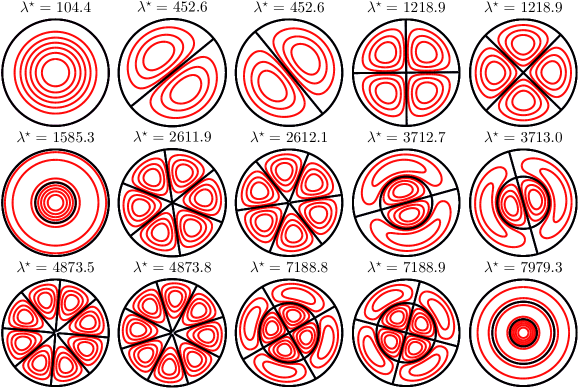
Figure 4: The contour lines of the first $15$ modes of the unclamped problem (3) on the unit disk. The nodal lines ($u^{\star}=0$) are plotted in black. Eigenfunctions are repeated according to their multiplicity.

For punctures away from the origin, we seek solutions of (1) with parameterized puncture sets to minimize the number of unknowns over which nonlinear iterations are processed. In the disk case, our first example is a single ring of punctures given explicitly as

$$\mathbf{x}_{j}=r\left(\cos\frac{2\pi j}{M},\sin\frac{2\pi j}{M}\right),\qquad j=1,\ldots,M.$$ (25)

There is now a single parameter $r$ over which various configurations can be investigated from $0<r<1$. From the eigenvalue $\lambda\approx 516.96$, which is the lowest positive solution of (22), we form an initial guess for the Newton iterations. Since our search pattern (25) is radially symmetric, the puncture strengths $\{\alpha_{j}\}_{j=1}^{M}$ can be assumed to be identical in this case.

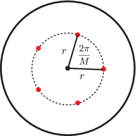
(a) Single puncture ring pattern

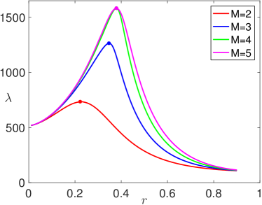
(b) The lowest eigenvalue against ring radius

Figure 5: Left: A disk with a single ring puncture configuration (red dots). Right: The lowest radially symmetric eigenvalue as a function of the puncture ring radius $r$. The integral equation (19) is discretized with $N=128$ boundary points.

In Fig. 5 we see that as the eigenvalue is varied, $\lambda$ attains a maximum value depending on the number of punctures and the radius of the ring. In Table 1, we display the maximum value of the lowest eigenvalue $\lambda_{c}$ and the critical radius $r_{c}$ of puncture ring where it is attained. The results in Table 1 are in good agreement with [38] and corroborate the observation that the maximum eigenvalue saturates as the number of puncture points $M$ increases.

To explain the saturation effect, we recall equation (5) that relates the puncture and puncture free modes. Consider a mode $(\lambda_{k}^{\star},u_{k}^{\star})$ of the puncture free eigenfunction problem (3) such that $u_{k}^{\star}(\mathbf{x}_{j})=0$, for $j=1,\ldots,M$. Then from (5) we have that $(\lambda-\lambda_{k}^{\star})\braket{u,u_{k}^{\star}}=0$. This implies that either $\lambda=\lambda_{k}^{\star}$ or $\braket{u,u_{k}^{\star}}=0$ so that if $u\to u^{\star}_{k}$, then $\lambda\to\lambda_{k}^{\star}$. From this we conclude that by centering punctures on the nodal set of a puncture free eigenfunction $u_{k}^{\star}$, then that eigenfunction becomes a mode of (1) thereby eliminating other modes form the spectrum.

$M$	$2$	$3$	$4$	$5$	$6$	$7$	$8$
$r_{c}$	$0.222$	$0.348$	$0.379$	$0.379$	$0.379$	$0.379$	$0.379$
$\lambda_{c}$	$734.96$	$1264.2$	$1581.5$	$1581.5$	$1581.5$	$1581.5$	$1581.5$

Table 1: The maximum value $\lambda_{c}$ of the lowest eigenvalue of the unit disk with a single ring of punctures. The values are obtained by numerical simulations with $N=128$ boundary points.

In this disk case with a single ring of punctures, saturation occurs when the punctures are placed on the nodal set of $u^{\star}_{0,1}(\mu^{\star}_{0,1}\rho)$—the mode with zero angular nodal lines and one radial nodal line. From (24), we see that the corresponding eigenvalue is $\lambda_{0,1}^{\star}=1581.7$ which agrees closely with the saturating value in Table 1. The critical radius $r_{c}$ is found by solving

$$u^{\star}_{0,1}(\mu^{\star}_{0,1}r_{c})=0\quad\Longrightarrow\quad r_{c}\approx 0.379,$$

which agrees closely with the numerical results in Table 1.

The practical importance of this phenomenon is that undesirable frequencies of the plate can be removed by specific placement of clamping locations. For example, the placement of five clamped points equally spaced on a circle of radius $r_{c}\approx 0.379$ yields that the lowest mode of (1) becomes $u^{\star}_{0,1}\approx 1585.3$, and the first four (including multiplicities) vibrational frequencies in Fig. 4 have been tuned out. For four equally spaced clamping points, the lowest mode would have been $\lambda^{\star}_{2,0}\approx 1218.9$ resulting in the lowest three modes being tuned out.

4.2 Rectangular Domain

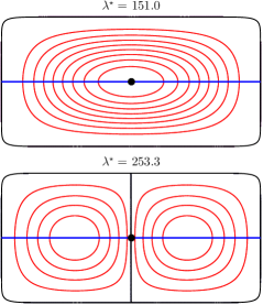
(a) The first two unclamped modes.

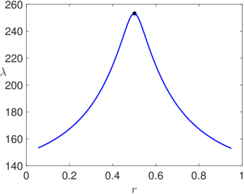
(b) The first clamped mode along the centerline

Figure 6: Results for the rectangular domain (26) with $a=\sqrt{2}$, $b=1/\sqrt{2}$ and a single clamped point on the horizontal axis. The eigenvalue attains its maximum when clamping is at the origin.

In this section, we consider rectangular domains and demonstrate a qualitative agreement with a previous study [23] on the localization of eigenfunctions of (1). We parameterize the boundary as

$$\partial\Omega=(x,y)=(a\,r(\theta)\cos\theta,b\,r(\theta)\sin\theta),\qquad\theta\in[0,2\pi),\qquad r(\theta)=\left[\cos^{p}\theta+\sin^{p}\theta\right]^{-\frac{1}{p}},$$ (26)

where $p$ is a parameter which regularizes the corners of the rectangle while $a$ and $b$ give the aspect ratio. We use $p=16$ in our calculations. Our first simulation investigates the effect of a single clamping location on the eigenvalue $\lambda$ of (1). We take a single clamped point and vary its location on the horizontal axis while calculating $\lambda(r)$ for $r\in(0,1)$ where $r=0$ and $r=1$ correspond to the left and right hand boundaries. In the curve Fig. 6(b) we see that the lowest eigenvalue attains a maximum at $r=1/2$ when the clamping occurs at the origin. The value of $\lambda$ at that peak corresponds to the second unclamped mode seen in eigenfunction of Fig. 6(a). Therefore a single clamping point placed at the center of the rectangle completely removes the first mode from the spectrum of (3).

(a) One clamped point.

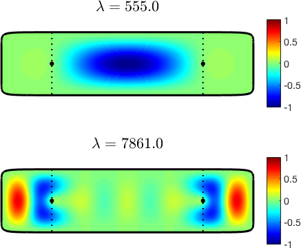
(b) Two clamped points.

Figure 7: Mode confinement effect with one (left panel) and two (right panel) point constraints on higher (bottom) and lower (top) modes of (1) in the rectangular domain (26) with $a=2$, $b=1/2$. Clamping occurs on the horizontal axis at locations $\pm(1.2,0)$. The simulations use $N=512$ discretization points of the domain’s boundary.

In our second simulation, we investigate the effect clamping points has on the eigenfunctions oscillations (cf. [23]). In Fig. 7 we display two modes for (1) for the rectangular domain with $a=2$, $b=1/2$ with one and two clamped points. The main observation is that a result of clamping is a confinement region, i.e. the eigenfunction is effectively zero on either the left or right of the clamping point.

4.3 Elliptical Domain

In this section, we consider equation (1) on the elliptical domain defined parametrically as

$$\partial\Omega=(x,y)=(a\cos\theta,b\sin\theta),\qquad\theta\in[0,2\pi).$$ (27)

As with the disk problem, the defect free eigenfunctions $u^{\star}$ satisfying equation (3) gives insight into the effect that puncturing will have on the modes. In Fig. 8, we display the first $15$ modes of (3) for $a=\frac{3}{2}$, $b=\frac{2}{3}$ with nodal lines. The choice $a=b^{-1}$ is made so that the ellipse has area $\pi$.

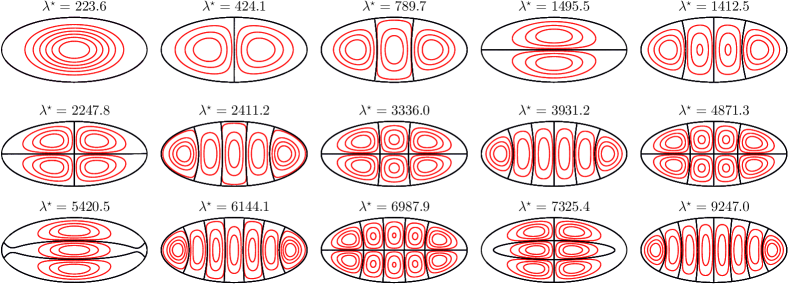
Figure 8: The first $15$ clamped modes of (3) of an ellipse (27) with $a=3/2$, $b=2/3$. The nodal lines ($u^{\star}=0$) are in black.

As with the disk domain, we determine solutions of (1) over one parameter families of puncture patterns. In this example we choose inscribed ellipses, circular patterns, and rectangular patterns. For the elliptical and rectangular cases, the aspect ratio of the puncture pattern is chosen to be the same as the outer ellipse and the pattern is stretched in a uniform way by a single parameter $r$ (cf. Fig. 9).

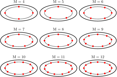
(a) Ellipse puncture patterns.

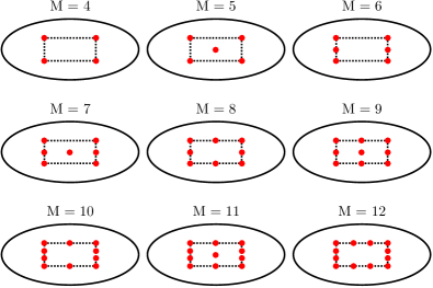
(b) Rectangular puncture patterns.

Figure 9: Elliptical and rectangular puncture patterns for $M=4,\ldots,12,$ inside an ellipse (27) with $a=3/2$, $b=2/3$. The aspect ratio of the patterns matches that of the outer ellipse.

The results for the puncture patterns corresponding to Fig. 9 and the circular pattern Fig. 5 are given in Fig. 10. The curves show that the pattern that generates the maximum eigenvalue varies for different $M$. The horizontal axis is a positive parameter $r$ which is a scale factor controlling the size of the pattern. The elliptical puncture pattern generates the largest eigenvalue for all $M$ tested except for $M=5$ where the rectangular patter generates a higher value. The circular pattern generally results in a lower maximum eigenvalue than the other patterns tested, expect in the $M=4$ case where the circular example generates a slightly larger value than the rectangle.

The discussion from the previous circular and rectangular examples, together with formula (5), suggest that clamping along the nodal lines of the unperturbed mode results in a maximum deviation of the eigenvalue $\lambda$ of (1). This suggests that the better performance of the elliptical pattern in maximizing the eigenvalue is that it more closely places punctures on the nodal lines (cf. Fig. 9) of $u^{\star}(\mathbf{x})$.

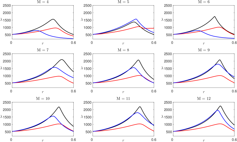
Figure 10: The first eigenvalue of (1) for the ellipse (27) with $a=3/2$, $b=2/3$ and $M=4,\ldots,12,$ punctures. Curves for rectangular (blue), elliptical (black) and circular (red) patterns.

4.4 Non-symmetric geometry

Here we consider the asymmetric domain whose boundary $\partial\Omega$ is specified parametrically as

$$\partial\Omega=(r(\theta)\cos\theta,r(\theta)\sin\theta),\qquad\theta\in[0,2\pi);\qquad r(\theta)=1+0.25\sin\theta+0.15\cos 3\theta,$$

and investigate the solution of (1) with a single clamped point. As in the previous examples, the first step is to consider the eigenvalues of the hole free problem (3). The first two modes are shown in Fig. 11(a).

To initiate Newton iterations for this example, we begin with a single clamped point near the boundary so that the unperturbed mode $\lambda^{\star}\approx 118.3$ in Fig. 11(a) provides a good initial guess for the system. From this start point, we vary the puncture location along a straight line (blue line in Fig. 11(a)) through the center of the domain to the opposing boundary. The maximum of this curve is attained when the clamping location coincides with the maximum of the first eigenfunction, occurring at the solid dot shown in Fig. 11(a).

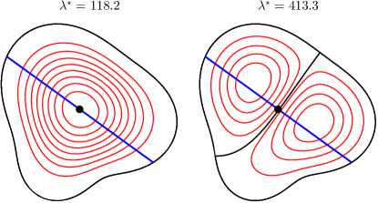
(a) The first and second unpunctured modes.

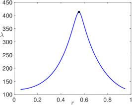
(b) The first punctured eigenvalue.

Figure 11: Panel (a): The first two modes of the hole free problem (3). Panel (b): The first eigenvalue of (1) for a clamped point located a distance $r$ along the blue line in panel (a).

In this example we again see that the first frequency can be tuned out of the vibrational characteristics of the plate by careful placement of just one clamping point.

4.5 Non-simply connected geometry

In this section, we consider a non-simply connected domain comprised of the unit disk with a circle of radius $0.2$ and center $(-0.3,0)$ removed. This multiply-connected domain has a confinement zone in the eigenfunction (see Fig. 12). Throughout this confinement zone (shaded region of Fig. 12(a)), the eigenfunction is very close to zero indicating again that small defects (holes, clamping points) cause a global perturbation to the modal characteristics in the fourth-order problem (1).

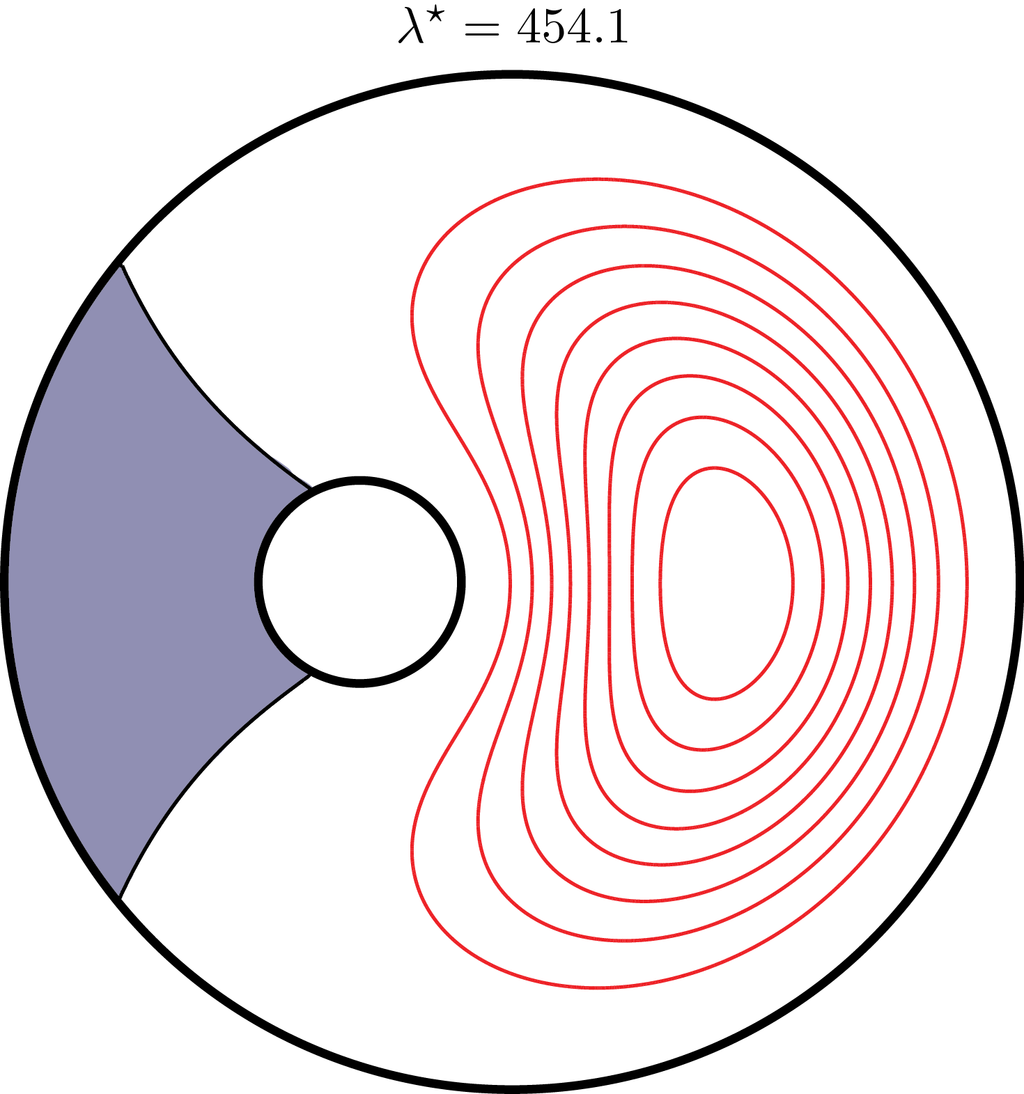
(a) Domain and first unclamped mode.

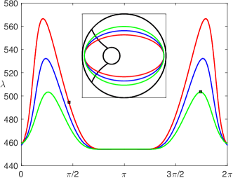
(b) Effect of clamping along an ellipse.

Figure 12: Non simply-connected domain example: Left: The first mode corresponding to $\lambda^{\star}=454.1$ with the shaded confinement zone in which $u^{\star}\approx 0$. Right: The clamped eigenvalue for a single point on inner ellipses with $a=0.95$ and $b=0.5$ (red curve), $0.6$ (blue curve), $0.7$ (green curve). The clamped modes corresponding to the black squares are shown in Fig. 13.

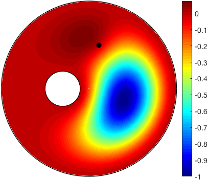
(a) $b=0.5$.

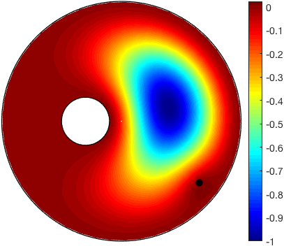
(b) $b=0.7$.

Figure 13: The clamped modes corresponding to solid squares in Fig. 12(b). The mode changes sign in the vicinity of the clamping point. Left: The single clamped point is $\mathbf{x}_{1}=(0.114,0.496)$ and $\lambda=494.5$. Right: The single clamped point is $\mathbf{x}_{1}=(0.648,-0.512)$ and $\lambda=503.4$.

To investigate the effect of clamping, we vary the location of a single clamped point along an inner ellipse with parameterization (27) for $a=0.95$ and the three values $b=0.5$, $0.6$, $0.7$. The results, displayed in Fig. 12(b), show the eigenvalue as a function of angular position on the ellipse. The flat region in the center of each curve corresponds to the transit of the clamped point through the confinement zone. In this region the eigenfunction is very close to zero ($u^{\star}\approx 0$), therefore the formula (5) shows that the eigenvalue should correspond to the unperturbed mode of Fig. 12(a).

In Fig. 13 we show two typical clamped modes which correspond to the particular clamping locations marked in Fig. 12(b). In each case a large confinement zone is seen to the left of the hole while the mode is also suppressed in the vicinity of the clamped point.

5 Conclusions

This paper has analyzed the modes of vibrations of thin elastic plates with multiple point constraints. We have developed and validated a novel boundary integral method for determining the eigenvalues of the fourth-order bi-Laplacian problem (1) with multiple clamped point constraints. This method is third-order accurate and can be easily applied to a variety of symmetric, asymmetric and multiply-connected geometries in two dimensions.

Our results indicate that the number and location of clamping points has two profound effects on the modes of vibrations of thin plates. First, by placing the clamping locations at the nodal lines of the unclamped eigenfunctions, certain eigenvalues can be removed from the spectrum of the problem. This implies that the vibrational characteristics of the plate can be manipulated or tuned by judicious placement of a small number clamping sites. A particularly important consequence of this effect in engineering applications is that undesirable frequencies of vibration can be completely removed. Second, clamping can have the effect of partitioning the plate into multiple subdomains in which vibrational modes are largely confined to a subset of those smaller spatial regions. This localization effect, previously seen only in rectangular plates with a single clamping location [23], has been observed here in other geometries and for multiple clamping locations.

There are many possibilities for future work that arise from this study. The order of the numerical method could be improved by adopting quadrature methods (cf. [2, 32]) suited to integrals with logarithmic singularities. In addition, the boundary integral equation could be more efficiently solved with a fast summation method such as the kernel-independent fast multipole method [51]. A more significant challenge is to develop a numerical method for the point constraint eigenvalue problem (1) which does not require the solution of a nonlinear system, such as (17), but still enforces the weak logarithmic singularity on the eigenfunction. This would eliminate the use of Newton’s method and the need to carefully control the initial conditions of the system. Such a method would easily accommodate a much larger number of clamping locations and allow for more reliable evaluation of the high frequency modes of (1).

Appendix A Kernels

The four kernels that appear in the integral equation (19) are $G_{11}=G_{1}$, $G_{12}=G_{2}$, $G_{21}=\partial{\mathbf{n}_{\mathbf{x}}}G_{1}$, and $G_{22}=\partial{\mathbf{n}_{\mathbf{x}}}G_{2}$. Expressions for $G_{11}$ and $G_{12}$ are in Section 2.3. Here we compute their normal derivatives with respect to the target point.

$$G_{21}=-\frac{1}{4\pi\mu^{2}} \left(-3\mu^{4}K_{0}(\mu\rho)\frac{(\mathbf{r}\cdot\mathbf{n})(\mathbf{r}\cdot\mathbf{n}_{\mathbf{x}})}{\rho^{2}}-12\mu^{3}K_{1}(\mu\rho)\frac{(\mathbf{r}\cdot\mathbf{n})(\mathbf{r}\cdot\mathbf{n}_{\mathbf{x}})}{\rho^{3}}+3\mu^{3}K_{1}(\mu\rho)\frac{(\mathbf{n}\cdot\mathbf{n}_{\mathbf{x}})}{\rho}\right.$$

$$\left.+2\mu^{4}K_{0}(\mu\rho)\frac{(\mathbf{r}\cdot\mathbf{n})^{3}(\mathbf{r}\cdot\mathbf{n}_{\mathbf{x}})}{\rho^{4}}+16\mu^{3}K_{1}(\mu\rho)\frac{(\mathbf{r}\cdot\mathbf{n})^{3}(\mathbf{r}\cdot\mathbf{n}_{\mathbf{x}})}{\rho^{5}}-6\mu^{3}K_{1}(\mu\rho)\frac{(\mathbf{r}\cdot\mathbf{n})^{2}(\mathbf{n}\cdot\mathbf{n}_{\mathbf{x}})}{\rho^{3}}\right.$$

$$\left.+6\mu^{2}K_{0}(\mu\rho)\frac{(\mathbf{n}\cdot\mathbf{n}_{\mathbf{x}})}{\rho^{2}}-24\mu^{2}K_{0}(\mu\rho)\frac{(\mathbf{r}\cdot\mathbf{n})(\mathbf{r}\cdot\mathbf{n}_{\mathbf{x}})}{\rho^{4}}-24\mu^{2}K_{0}(\mu\rho)\frac{(\mathbf{r}\cdot\mathbf{n})^{2}(\mathbf{n}\cdot\mathbf{n}_{\mathbf{x}})}{\rho^{4}}\right.$$

$$\left.+48\mu^{2}K_{0}(\mu\rho)\frac{(\mathbf{r}\cdot\mathbf{n})^{3}(\mathbf{r}\cdot\mathbf{n}_{\mathbf{x}})}{\rho^{6}}+96\mu K_{1}(\mu\rho)\frac{(\mathbf{r}\cdot\mathbf{n})^{3}(\mathbf{r}\cdot\mathbf{n}_{\mathbf{x}})}{\rho^{7}}-48\mu K_{1}(\mu\rho)\frac{(\mathbf{r}\cdot\mathbf{n})^{2}(\mathbf{n}\cdot\mathbf{n}_{\mathbf{x}})}{\rho^{5}}\right.$$

$$\left.-48\mu K_{1}(\mu\rho)\frac{(\mathbf{r}\cdot\mathbf{n})(\mathbf{r}\cdot\mathbf{n}_{\mathbf{x}})}{\rho^{5}}+12\mu K_{1}(\mu\rho)\frac{(\mathbf{n}\cdot\mathbf{n}_{\mathbf{x}})}{\rho^{3}}\right)$$

$$-\frac{1}{8\mu^{2}} \left(-3\mu^{4}Y_{0}(\mu\rho)\frac{(\mathbf{r}\cdot\mathbf{n})(\mathbf{r}\cdot\mathbf{n}_{\mathbf{x}})}{\rho^{2}}+12\mu^{3}Y_{1}(\mu\rho)\frac{(\mathbf{r}\cdot\mathbf{n})(\mathbf{r}\cdot\mathbf{n}_{\mathbf{x}})}{\rho^{3}}-3\mu^{3}Y_{1}(\mu\rho)\frac{(\mathbf{n}\cdot\mathbf{n}_{\mathbf{x}})}{\rho}\right.$$

$$\left.+2\mu^{4}Y_{0}(\mu\rho)\frac{(\mathbf{r}\cdot\mathbf{n})^{3}(\mathbf{r}\cdot\mathbf{n}_{\mathbf{x}})}{\rho^{4}}-16\mu^{3}Y_{1}(\mu\rho)\frac{(\mathbf{r}\cdot\mathbf{n})^{3}(\mathbf{r}\cdot\mathbf{n}_{\mathbf{x}})}{\rho^{5}}+6\mu^{3}Y_{1}(\mu\rho)\frac{(\mathbf{r}\cdot\mathbf{n})^{2}(\mathbf{n}\cdot\mathbf{n}_{\mathbf{x}})}{\rho^{3}}\right.$$

$$\left.-6\mu^{2}Y_{0}(\mu\rho)\frac{(\mathbf{n}\cdot\mathbf{n}_{\mathbf{x}})}{\rho^{2}}+24\mu^{2}Y_{0}(\mu\rho)\frac{(\mathbf{r}\cdot\mathbf{n})(\mathbf{r}\cdot\mathbf{n}_{\mathbf{x}})}{\rho^{4}}+24\mu^{2}Y_{0}(\mu\rho)\frac{(\mathbf{r}\cdot\mathbf{n})^{2}(\mathbf{n}\cdot\mathbf{n}_{\mathbf{x}})}{\rho^{4}}\right.$$

$$\left.-48\mu^{2}Y_{0}(\mu\rho)\frac{(\mathbf{r}\cdot\mathbf{n})^{3}(\mathbf{r}\cdot\mathbf{n}_{\mathbf{x}})}{\rho^{6}}+96\mu Y_{1}(\mu\rho)\frac{(\mathbf{r}\cdot\mathbf{n})^{3}(\mathbf{r}\cdot\mathbf{n}_{\mathbf{x}})}{\rho^{7}}-48\mu Y_{1}(\mu\rho)\frac{(\mathbf{r}\cdot\mathbf{n})^{2}(\mathbf{n}\cdot\mathbf{n}_{\mathbf{x}})}{\rho^{5}}\right.$$

$$\left.-48\mu Y_{1}(\mu\rho)\frac{(\mathbf{r}\cdot\mathbf{n})(\mathbf{r}\cdot\mathbf{n}_{\mathbf{x}})}{\rho^{5}}+12\mu Y_{1}(\mu\rho)\frac{(\mathbf{n}\cdot\mathbf{n}_{\mathbf{x}})}{\rho^{3}}\right).$$

$$G_{22}=-\frac{1}{4\pi} \left(8K_{0}(\mu\rho)\frac{(\mathbf{r}\cdot\mathbf{n})^{2}(\mathbf{r}\cdot\mathbf{n}_{\mathbf{x}})}{\rho^{4}}+\frac{16}{\mu}K_{1}(\mu\rho)\frac{(\mathbf{r}\cdot\mathbf{n})^{2}(\mathbf{r}\cdot\mathbf{n}_{\mathbf{x}})}{\rho^{5}}-4K_{0}(\mu\rho)\frac{(\mathbf{r}\cdot\mathbf{n})(\mathbf{n}\cdot\mathbf{n}_{\mathbf{x}})}{\rho^{2}}\right.$$

$$\left.-\frac{8}{\mu}K_{1}(\mu\rho)\frac{(\mathbf{r}\cdot\mathbf{n})(\mathbf{n}\cdot\mathbf{n}_{\mathbf{x}})}{\rho^{3}}-\mu K_{1}(\mu\rho)\frac{(\mathbf{r}\cdot\mathbf{n}_{\mathbf{x}})}{\rho}-\frac{4}{\mu}K_{1}(\mu\rho)\frac{(\mathbf{r}\cdot\mathbf{n}_{\mathbf{x}})}{\rho^{3}}\right.$$

$$\left.-2K_{0}(\mu\rho)\frac{(\mathbf{r}\cdot\mathbf{n}_{\mathbf{x}})}{\rho^{2}}+2\mu K_{1}(\mu\rho)\frac{(\mathbf{r}\cdot\mathbf{n})^{2}(\mathbf{r}\cdot\mathbf{n}_{\mathbf{x}})}{\rho^{3}}\right)$$

$$+\frac{1}{8} \left(8Y_{0}(\mu\rho)\frac{(\mathbf{r}\cdot\mathbf{n})^{2}(\mathbf{r}\cdot\mathbf{n}_{\mathbf{x}})}{\rho^{4}}-\frac{16}{\mu}Y_{1}(\mu\rho)\frac{(\mathbf{r}\cdot\mathbf{n})^{2}(\mathbf{r}\cdot\mathbf{n}_{\mathbf{x}})}{\rho^{5}}-4Y_{0}(\mu\rho)\frac{(\mathbf{r}\cdot\mathbf{n})(\mathbf{n}\cdot\mathbf{n}_{\mathbf{x}})}{\rho^{2}}\right.$$

$$\left.+\frac{8}{\mu}Y_{1}(\mu\rho)\frac{(\mathbf{r}\cdot\mathbf{n})(\mathbf{n}\cdot\mathbf{n}_{\mathbf{x}})}{\rho^{3}}-\mu Y_{1}(\mu\rho)\frac{(\mathbf{r}\cdot\mathbf{n}_{\mathbf{x}})}{\rho}+\frac{4}{\mu}Y_{1}(\mu\rho)\frac{(\mathbf{r}\cdot\mathbf{n}_{\mathbf{x}})}{\rho^{3}}\right.$$

$$\left.-2Y_{0}(\mu\rho)\frac{(\mathbf{r}\cdot\mathbf{n}_{\mathbf{x}})}{\rho^{2}}+2\mu Y_{1}(\mu\rho)\frac{(\mathbf{r}\cdot\mathbf{n})^{2}(\mathbf{r}\cdot\mathbf{n}_{\mathbf{x}})}{\rho^{3}}\right).$$

References

- [1] M. Abramowitz and I. Stegun. Handbook of Mathematical Functions with Formulas, Graphs and Mathematical Tables. Dover, New York, 1964.
- [2] B. K. Alpert. Hybrid Gauss-Trapezoidal Quadrature Rules. SIAM Journal on Scientific Computing, 20:1551–1584, 1999.
- [3] Carlos J. S. Alves and Pedro R. S. Antunes. The method of fundamental solutions applied to the calculation of eigensolutions for 2d plates. International Journal for Numerical Methods in Engineering, 77(2):177–194, 2009.
- [4] I.V. Andrianov, V.V. Danishevs’kyy, and A.L. Kalamkarov. Asymptotic analysis of perforated plates and membranes. part 2: Static and dynamic problems for large holes. International Journal of Solids and Structures, 49(2):311–317, 2012.
- [5] Noureddine Atalla and Franck Sgard. Modeling of perforated plates and screens using rigid frame porous models. Journal of Sound and Vibration, 303(1-2):195–208, 2007.
- [6] Arnd Bäcker. Numerical aspects of eigenvalue and eigenfunction computations for chaotic quantum systems. In The mathematical aspects of quantum maps, pages 91–144. Springer, 2003.
- [7] A. H. Barnett. Perturbative Analysis of the Method of Particular Solutions for Improved Inclusion of High-Lying Dirichlet Eigenvalues. SIAM Journal on Numerical Analysis, 47(3):1952–1970, 2009.
- [8] Alex Barnett and Andrew Hassell. Fast Computation of High-Frequency Dirichlet Eigenmodes via Spectral Flow of the Interior Neumann-to-Dirichlet Map. Communications on Pure and Applied Mathematics, 67(3):351–407, 2014.
- [9] Timo Betcke. A GSVD formulation of a domain decomposition method for planar eigenvalue problems. IMA Journal of Numerical Analysis, 27(3):451–478, 2007.
- [10] B. M. Brown, E. B. Davies, P. K. Jimack, and M. D. Mihajlović. A numerical investigation of the solution of a class of fourth order eigenvalue problems. Proceeding of the Royal Society A: Mathematical Physical & Engineering Sciences, 456(1998):1505–1521, 2000.
- [11] K.A. Burgemeister and C.H. Hansen. Calculating resonance frequencies of perforated panels. Journal of Sound and Vibration, 196(4):387–399, 1996.
- [12] A. Campbell and S.A. Nazarov. Asymptotics of eigenvalues of a plate with small clamped zone. Positivity, 5:275–295, 2001.
- [13] Gilles Chardon and Laurent Daudet. Low-complexity computation of plate eigenmodes with vekua approximations and the method of particular solutions. Computational Mechanics, 52(5):983–992, 2013.
- [14] C. Coffman. On the structure of solutions which satisfy the clamped plate conditions on a right angle. SIAM Journal on Mathematical Analysis, 13(5):746–757, 1982.
- [15] C. V. Coffman, R. J. Duffin, and D. H. Shaffer. The fundamental mode of vibration of a clamped annular plate is not of one sign. Constructive Approaches to Mathematical Models (Proc. Conf. in honor of R. J. Duffin, Pittsburgh, PA.), pages 267–277, 1979.
- [16] Charles V Coffman and Richard J Duffin. On the fundamental eigenfunctions of a clamped punctured disk. Advances in Applied Mathematics, 13(2):142–151, 1992.
- [17] Jean Descloux and Michael Tolley. An accurate algorithm for computing the eigenvalues of a polygonal membrane. Computer Methods in Applied Mechanics and Engineering, 39(1):37–53, 1983.
- [18] Tobin A. Driscoll. Eigenmodes of Isospectral Drums. SIAM Review, 39(1):1–17, 1997.
- [19] Toby Driscoll. Frequencies of a Drum. http://www.chebfun.org/examples/ode-eig/Drum.html.
- [20] Mario Durán, Jean-Claude Nédélec, and Sebastián Ossandón. An Efficient Galerkin BEM to Compute High Acoustic Eigenfrequencies. Journal of Vibration and Acoustics, 131(3):031001, 2009.
- [21] Lawrence C. Evans. Partial Differential Equations: Second Edition. American Mathematical Society, 2010.
- [22] P. Farkas. Mathematical Foundations for Fast Algorithms for the Biharmonic Equation. PhD thesis, University of Chicago, 1989.
- [23] Marcel Filoche and Svitlana Mayboroda. Strong localization induced by one clamped point in thin plate vibrations. Phys. Rev. Lett., 103:254301, Dec 2009.
- [24] M. Flucher. Approximation of dirichlet eigenvalues on domains with small holes. Journal of Mathematical Analysis and Applications, 193(1):169–199, 1995.
- [25] L. Fox, P. Henrici, and C. Moler. Approximations and bounds for eigenvalues of elliptic operators. SIAM Journal on Numerical Analysis, 4(1):89–102, 1967.
- [26] Filippo Gazzola, Hans-Christoph Grunau, and Guido Sweers. Polyharmonic Boundary Value Problems. Springer, 2010.
- [27] David Gilbarg and Neil S. Trudinger. Elliptic Partial Differential Equations of Second Order. Springer, 1998.
- [28] Hans-Christoph Grunau and Guido Sweers. In any dimension a “clamped plate” with a uniform weight may change sign. Nonlinear Analysis: Theory, Methods and Applications, 97(0):119 – 124, 2014.
- [29] Kazuo Ishihara. A mixed finite element method for the biharmonic eigenvalue problems of plate bending. Publications of the Research Institute for Mathematical Sciences, 14(2), 1978.
- [30] L. Jaouen and F.-X. Bécot. Acoustical characterization of perforated facings. The Journal of the Acoustical Society of America, 129(3):1400–1406, 2011.
- [31] Shidong Jiang, Mary-Catherine A. Kropinski, and Bryan D. Quaife. Second kind integral equation formulations for the modified biharmonic equation and its applications. Journal of Computational Physics, 249:113–126, 2013.
- [32] Sharad Kapur and Vladimir Rokhlin. High-Order Corrected Trapezoidal Quadrature Rules for Singular Functions. SIAM Journal on Numerical Analysis, 34(4):1331–1356, 1997.
- [33] A. Karageorghis. The Method of Fundamental Solutions for the Calculation of the Eigenvalues of the Helmholtz Equation. Applied Mathematics Letters, 14:837–842, 2011.
- [34] T. Kolokolnikov, M. S. Titcombe, and M. J. Ward. Optimizing the fundamental neumann eigenvalue for the laplacian in a domain with small traps. European Journal of Applied Mathematics, 16:161–200, 4 2005.
- [35] K. Krishnakumar and G. Venkatarathnam. Transient testing of perforated plate matrix heat exchangers. Cryogenics, 43(2):101–109, 2003.
- [36] M. C. Kropinski, A. E. Lindsay, and M. J. Ward. Asymptotic analysis of localized solutions to some linear and nonlinear biharmonic eigenvalue problems. Studies in Applied Mathematics, 126(4):347–408, 2011.
- [37] W. M. Lee and J. T. Chen. Free vibration analysis of circular plates with multiple circular holes using indirect biem and addition theorem. J. Appl. Mechanics, 78(1), 2010.
- [38] A. E. Lindsay, W. Hao, and A. J. Sommese. Vibrations of thin plates with small clamped patches. Proceedings of the Royal Society of London A: Mathematical, Physical and Engineering Sciences, 471(2184), 2015.
- [39] A. E. Lindsay, M. J. Ward, and T. Kolokolnikov. The transition to point constraint in a mixed biharmonic eigenvalue problem. SIAM Journal on Applied Mathematics, 75(3):1193–1224, 2015.
- [40] L. Marin and D. Lesnic. The Method of Fundamental Solutions for Inverse Boundary Value Problems Associated with the Two-Dimensional Biharmonic Equation. Mathematical and Computer Modelling, 42:261–278, 2005.
- [41] Michael J. Nilles, Myron E. Calkins, Michael L. Dingus, and John B. Hendricks. Heat transfer and flow friction in perforated plate heat exchangers. Experimental Thermal and Fluid Science, 10(2):238–247, 1995. Aerospace Heat Exchanger Technology.
- [42] Shin Ozawa. Singular variation of domains and eigenvalues of the laplacian. Duke Mathematical Journal, 48(4):767–778, 12 1981.
- [43] R. B. Platte and T. A. Driscoll. Computing Eigenmodes of Elliptic Operators Using Radial Basis Functions. Computers and Matematics with Applications, 48:561–576, 2004.
- [44] J. N. Reddy. Theory and Analysis of Plates and Shells. CRC Press, Taylor and Francis, 2007.
- [45] O. Steinbach and G. Unger. A boundary element method for the Dirichlet eigenvalue problem of the Laplace operator. Numerische Mathematik, 113(2):281–298, 2009.
- [46] G. Sweers. When is the first eigenfunction for the clamped plate equation of fixed sign? Electronic J. Differ. Equ. Conf. Southwest Texas State Univ., San Marcos, Texas, 6:285–296, 2001.
- [47] G. Venkatarathnam. Effectiveness- relationship in perforated plate matrix heat exchangers. Cryogenics, 36(4):235–241, 1996.
- [48] Chunqi Wang, Li Cheng, Jie Pan, and Ganghua Yu. Sound absorption of a micro-perforated panel backed by an irregular-shaped cavity. The Journal of the Acoustical Society of America, 127(1):238–246, 2010.
- [49] M. Ward, W. Heshaw, and J. Keller. Summing logarithmic expansions for singularly perturbed eigenvalue problems. SIAM Journal on Applied Mathematics, 53(3):799–828, 1993.
- [50] M. Ward and J. Keller. Strong localized perturbations of eigenvalue problems. SIAM Journal on Applied Mathematics, 53(3):770–798, 1993.
- [51] Lexing Ying, George Biros, and Denis Zorin. A kernel-independent adaptive fast multipole algorithm in two and three dimensions. J. Comput. Phys., 196(2):591–626, May 2004.
- [52] Y.B. Zhao, G.W. Wei, and Y. Xiang. Plate vibration under irregular internal supports. International Journal of Solids and Structures, 39(5):1361 – 1383, 2002.