The sign of the dipole-dipole potential by axion exchange

Abstract

We calculate a dipole-dipole potential between fermions mediated by a light pseudoscalar, axion, paying a particular attention to the overall sign. While the sign of the potential is physical and important for experiments to discover or constrain the axion coupling to fermions, there is often a sign error in the literature. The purpose of this short note is to clarify the sign issue of the axion-mediated dipole-dipole potential. As a by-product, we find a sign change of the dipole-dipole potenital due to the different spin of the mediating particle.

1 Introduction

The exchange of a light particle gives rise to a force between other particles. One of such light particles is a pseudo Nambu-Goldstone boson, an axion, which appears in the Peccei-Quinn solution to the strong CP problem [1, 2, 3, 4]. The axion and axion-like particles have been searched for in many experiments (see e.g. Refs. [5, 6, 7, 8, 9] for recent reviews).

The axion or axion-like particle is generically coupled to nucleons and leptons, and the axion exchange induces a spin-dependent force between them, which has been constrained by many experiments [10]. Furthermore, there have been proposed many axion search experiments, some of which aim to measure the spin-dependent force due to axion exchange (e.g. [11]). Therefore, it is important to unambiguously understand the relation between the axion coupling and the observables.

In this short note we calculate a dipole-dipole potential between fermions mediated by an axion, paying a particular attention to the overall sign. The sign of the potential is physical and therefore important for experiments to discover or constrain the axion coupling to fermions. In particular, the most challenging part of experiments searching for such axion-mediated dipole-dipole potential is to shield the standard magnetic dipole-dipole interaction to an extremely high degree. The experimental limits are therefore sensitive to the sign of the potential as well as the residual magnetic dipole-dipole interaction. We note however that there is often a sign error in the literature, including the seminal paper [12] on the axion-exchange potentials between fermions. Also, some of the experiments seem to use the potential with a wrong sign (e.g. [13, 14, 15]). The sign issue may not affect the experimental limits on the spin-dependent force as long as the estimated limit is symmetric about zero. However, as a matter of fact, the sign is essential to claim a discovery of such a new force in future experiments.

The purpose of this short note is to clarify the sign issue of the dipole-dipole potential induced by axion exchange, and to eliminate the possibility that the sign error mediates to future experiments searching for such an anomalous force.

2 Scalar exchange potential

As an exercise, let us first consider a case where both fermions $\psi_{1}$ and $\psi_{2}$ interact with a real scalar $\phi$ through Yukawa interactions. The Lagrangian is given by

$$\mathcal{L}=\frac{1}{2}\partial_{\mu}\phi\partial^{\mu}\phi-\frac{1}{2}m_{\phi}^{2}\phi^{2}+\sum_{j=1,2}\left(\bar{\psi}_{j}(i\gamma^{\mu}\partial_{\mu}-M_{j})\psi_{j}-g_{Sj}\phi\,\bar{\psi}_{j}\psi_{j}\right),$$ (1)

where $m_{\phi}$ and $M_{j}$ are the mass of $\phi$ and $\psi_{j}$, respectively, and $g_{Sj}$ is a Yukawa coupling between $\phi$ and $\psi_{j}$. Here and in what follows we adopt the convention and notation used in the textbook by Peskin and Schroeder [16], except for the representation of the gamma matrices and the normalization of the spinors. We adopt the Dirac representation of the gamma matrices,

$$\gamma^{0}=\left(\begin{array}[]{cc}1&0\\ 0&-1\end{array}\right),~{}~{}\gamma^{i}=\left(\begin{array}[]{cc}0&\sigma^{i}\\ -\sigma^{i}&0\end{array}\right),~{}{\rm and}~{}\gamma_{5}=\left(\begin{array}[]{cc}0&1\\ 1&0\end{array}\right),~{}$$ (2)

where $\sigma^{i}$ are the Pauli matrices.

The vertex factor of the Yukawa interaction is then given by

$$(-i)g_{Sj}.$$ (3)

The scattering amplitude for $\psi_{1}(p_{1})\psi_{2}(p_{2})\to\psi_{1}(p_{1}^{\prime})\psi_{2}(p_{2}^{\prime})$ mediated by the scalar $\phi$ (see Fig. 1) is expressed as

$$i\mathcal{M}=\bar{u}_{1}^{s_{1}^{\prime}}(p_{1}^{\prime})(-ig_{S1})u_{1}^{s_{1}}(p_{1})\frac{i}{q^{2}-m_{\phi}^{2}}\bar{u}_{2}^{s_{2}^{\prime}}(p_{2}^{\prime})(-ig_{S2})u_{2}^{s_{2}}(p_{2}).$$ (4)

Here $q\equiv p_{1}^{\prime}-p_{1}=-(p_{2}^{\prime}-p_{2})$ is the momentum transfer between the two fermions, and the superscripts $s_{1}$, $s_{1}^{\prime}$, $s_{2}$ and $s_{2}^{\prime}$ denote the spin of each fermion. We adopt the non-relativistic normalization condition ${u_{j}^{s^{\prime}}}^{\dagger}(p)u_{j}^{s}(p)=\delta_{s,s^{\prime}}$ (no summation over $j$), which is different from the usual relativistic normalization, ${u_{j}^{s^{\prime}}}^{\dagger}(p)u_{j}^{s}(p)=2E\,\delta_{s,s^{\prime}}$, where $p=(E,\vec{p})$. With the non-relativistic normalization, the plane wave solution is given by

$$u_{j}^{s}(p)=\sqrt{\frac{E+M_{j}}{2E}}\left(\chi_{s},\,\frac{\vec{\sigma}\cdot\vec{p}}{E+M_{j}}\chi_{s}\right)^{\mathrm{T}}\simeq\left(\chi_{s},\,\frac{\vec{\sigma}\cdot\vec{p}}{2M_{j}}\chi_{s}\right)^{\mathrm{T}},$$ (5)

where $\chi_{s}$ is a two component spinor satisfying $\chi^{\dagger}_{s^{\prime}}\chi_{s}=\delta_{s,s^{\prime}}$, and we have taken the non-relativistic limit, $E\approx M_{j}$, in the second equality. Substituting this solution into (4), one obtains

$$i\mathcal{M}\simeq-i\frac{g_{S1}g_{S2}}{(q^{0})^{2}-|\vec{q}|^{2}-m_{\phi}^{2}}\delta_{s_{1},s_{1}^{\prime}}\delta_{s_{2},s_{2}^{\prime}}\simeq i\frac{g_{S1}g_{S2}}{|\vec{q}|^{2}+m_{\phi}^{2}}\delta_{s_{1},s_{1}^{\prime}}\delta_{s_{2},s_{2}^{\prime}},$$ (6)

where we have used, $|q^{0}|\ll|\vec{q}|$, in the non-relativistic limit in the second equality.

In general, the position-space potential can be obtained by taking the Fourier transform of the momentum-space amplitude with respect to the momentum transfer $\vec{q}$. In the case at hand, it is given by

$$V(\vec{r}) =-\int\frac{d^{3}q}{(2\pi)^{3}}e^{i\vec{q}\cdot\vec{r}}\left(\frac{g_{S1}g_{S2}}{|\vec{q}|^{2}+m_{\phi}^{2}}\right)$$ (7)

$$=-\frac{g_{S1}g_{S2}}{4\pi r}e^{-m_{\phi}r}$$ (8)

This result is of course consistent with Refs. [12] and [17] and many other literatures.

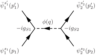
(a) Scalar exchange diagram

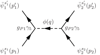
(b) Pseudoscalar exchange diagram

Figure 1: Feynman diagrams for fermion scattering mediated by (a) scalar and (b) pseudo scalar, respectively.

3 Pseudoscalar exchange potential

Next, let us go on to another type of interaction involving a pseudoscalar $\phi$. The Lagrangian is given by

$$\mathcal{L}=\frac{1}{2}\partial_{\mu}\phi\partial^{\mu}\phi-\frac{1}{2}m_{\phi}^{2}\phi^{2}+\sum_{j=1,2}\left(\bar{\psi}_{j}(i\gamma^{\mu}\partial_{\mu}-M_{j})\psi_{j}-ig_{Pj}\phi\,\bar{\psi}_{j}\gamma_{5}\psi_{j}\right),$$ (9)

where $g_{Pj}$ is a real coupling constant between $\phi$ and $\psi_{j}$. Note that the imaginary unity $i$ is included in the last term to make $g_{Pj}$ real. The vertex factor of the above interaction is

$$(-i)ig_{Pj}\gamma_{5}=g_{Pj}\gamma_{5}.$$ (10)

Then the scattering amplitude for $\psi_{1}(p_{1})\psi_{2}(p_{2})\to\psi_{1}(p_{1}^{\prime})\psi_{2}(p_{2}^{\prime})$ mediated by the pseudoscalar (see Fig. 1) is given by

$$i\mathcal{M}=\bar{u}_{1}^{s_{1}^{\prime}}(p_{1}^{\prime})g_{P1}\gamma_{5}u_{1}^{s_{1}}(p_{1})\frac{i}{q^{2}-m_{\phi}^{2}}\bar{u}_{2}^{s_{2}^{\prime}}(p_{2}^{\prime})g_{P2}\gamma_{5}u_{2}^{s_{2}}(p_{2}).$$ (11)

Using the plane wave solution (5), we can calculate the matrix element

$$\bar{u}_{1}^{s_{1}^{\prime}}(p_{1}^{\prime})\gamma_{5}u_{1}^{s_{1}}(p_{1}) \simeq\chi_{s_{1}^{\prime}}^{{\dagger}}\left(\frac{\vec{\sigma}}{2M_{1}}\cdot(\vec{p_{1}}-\vec{p_{1}}^{\prime})\right)\chi_{s_{1}},$$ (12)

$$\bar{u}_{2}^{s_{2}^{\prime}}(p_{2}^{\prime})\gamma_{5}u_{2}^{s_{2}}(p_{2}) \simeq\chi_{s_{2}^{\prime}}^{{\dagger}}\left(\frac{\vec{\sigma}}{2M_{2}}\cdot(\vec{p_{2}}-\vec{p_{2}}^{\prime})\right)\chi_{s_{2}},$$ (13)

and the amplitude becomes

$$i\mathcal{M} \simeq i\frac{g_{P1}g_{P2}}{q^{2}-m_{\phi}^{2}}\frac{\left(\chi^{\dagger}_{s_{1}^{\prime}}(\vec{\sigma}\cdot(-\vec{q}))\chi_{s_{1}}\right)\left(\chi^{{\dagger}}_{s_{2}^{\prime}}(\vec{\sigma}\cdot\vec{q})\chi_{s_{2}}\right)}{4M_{1}M_{2}},$$ (14)

$$\simeq i\frac{g_{P1}g_{P2}}{|\vec{q}|^{2}+m_{\phi}^{2}}\frac{\left(\chi^{\dagger}_{s_{1}^{\prime}}(\vec{\sigma}\cdot\vec{q})\chi_{s_{1}}\right)\left(\chi^{{\dagger}}_{s_{2}^{\prime}}(\vec{\sigma}\cdot\vec{q})\chi_{s_{2}}\right)}{4M_{1}M_{2}},$$ (15)

where we have taken the nonrelativistic limit in the second equality. Then, by taking the Fourier transform of the amplitude, we obtain

$$V(\vec{r}) =-\int\frac{d^{3}q}{(2\pi)^{3}}e^{i\vec{q}\cdot\vec{r}}\left[\frac{g_{P1}g_{P2}}{|\vec{q}|^{2}+m_{\phi}^{2}}\frac{(\vec{{S}}_{1}\cdot\vec{q})(\vec{{S}}_{2}\cdot\vec{q})}{M_{1}M_{2}}\right],$$ (16)

$$=\frac{g_{P1}g_{P2}}{M_{1}M_{2}}(\vec{{S}}_{1}\cdot\vec{\nabla})(\vec{{S}}_{2}\cdot\vec{\nabla})\int\frac{d^{3}q}{(2\pi)^{3}}\frac{1}{|\vec{q}|^{2}+m_{\phi}^{2}}e^{i\vec{q}\cdot\vec{r}},$$ (17)

$$=\frac{g_{P1}g_{P2}}{M_{1}M_{2}}(\vec{{S}}_{1}\cdot\vec{\nabla})(\vec{{S}}_{2}\cdot\vec{\nabla})\left(\frac{e^{-m_{\phi}r}}{4\pi r}\right),$$ (18)

where $\vec{{S}}_{1}$ and $\vec{{S}}_{2}$ are the spin operators of the fermions $\psi_{1}$ and $\psi_{2}$, respectively. In the literature, the spin operators are often represented by $\vec{\sigma}_{1}$ and $\vec{\sigma}_{2}$, and they are related as $\vec{{S}}_{1}=\vec{\sigma}_{1}/2$ and $\vec{{S}}_{2}=\vec{\sigma}_{2}/2$. Finally, using the formula

$$\nabla_{i}\nabla_{j}\left(\frac{e^{-m_{\phi}r}}{r}\right)=-e^{-m_{\phi}r}\left[\delta_{ij}\left(\frac{m_{\phi}}{r^{2}}+\frac{1}{r^{3}}+\frac{4\pi}{3}\delta^{3}(r)\right)-\hat{r}_{i}\hat{r}_{j}\left(\frac{m_{\phi}^{2}}{r}+\frac{3m_{\phi}}{r^{2}}+\frac{3}{r^{3}}\right)\right],$$ (19)

we arrive at the dipole-dipole potential induced by axion exchange,

$$V(\vec{r}) =-\frac{g_{P1}g_{P2}\exp(-m_{\phi}r)}{4\pi M_{1}M_{2}}\left[(\vec{{S}}_{1}\cdot\vec{{S}}_{2})\left(\frac{m_{\phi}}{r^{2}}+\frac{1}{r^{3}}+\frac{4\pi}{3}\delta^{3}(r)\right)\right.$$

$$~{}~{}~{}~{}~{}~{}~{}~{}~{}~{}~{}~{}~{}~{}~{}~{}~{}~{}~{}~{}~{}~{}~{}~{}~{}~{}~{}~{}~{}~{}~{}~{}~{}~{}\left.-(\vec{{S}}_{1}\cdot\hat{r})(\vec{{S}}_{2}\cdot\hat{r})\left(\frac{m_{\phi}^{2}}{r}+\frac{3m_{\phi}}{r^{2}}+\frac{3}{r^{3}}\right)\right],$$ (20)

where $\hat{r}\equiv\vec{r}/r$ is the unit vector. In the massless limit, we obtain

$$V(\vec{r}) \to-\frac{g_{P1}g_{P2}}{4\pi M_{1}M_{2}r^{3}}\left[\vec{{S}}_{1}\cdot\vec{{S}}_{2}-3(\vec{{S}}_{1}\cdot\hat{r})(\vec{{S}}_{2}\cdot\hat{r})\right],~{}~{}~{}~{}~{}~{}(m_{\phi}\to 0)$$ (21)

where we have dropped the contact term. The form of the potential in the massless limit should be compared with the standard magnetic dipole-dipole interaction,

$$H_{\mu\mu}=-\frac{3(\vec{\mu}_{1}\cdot\hat{r})(\vec{\mu}_{2}\cdot\hat{r})-\vec{\mu}_{1}\cdot\vec{\mu}_{2}}{4\pi r^{3}},$$ (22)

where $\vec{\mu}_{1}$ and $\vec{\mu}_{2}$ are the magnetic moments and we have omitted the Fermi contact term. The magnetic moment for an elementary Dirac particle is related to its spin as

$$\vec{\mu}=g\frac{e}{2m}\vec{{S}},$$ (23)

where $m$ and $g$ are the mass and $g$-factor of the particle, respectively. Notice the overall sign difference between (22) and (21) when $g_{P1}=g_{P2}$.

The above result (20) (and (21)) is consistent with Ref. [17], and with Ref. [19] in the limit of $m_{\phi}\to 0$. It is also consistent with the one (neutral) pion exchange potential between nucleons [20]. On the other hand, the results in e.g. Refs. [21, 12] have an opposite sign.

The sign of the potential is physical, therefore it is important for experiments to discover or constrain the axion couplings to fermions. Unfortunately, there is often the sign error in the literature (including the equation in the header of the limit on invisible axion electron coupling in PDG [10]). So far, the axion-mediated dipole-dipole potential is only limited by experiments, and the sign error does not change the results unless the estimated error is antisymmetric about the sign of the potential. However, as a matter of fact, the sign is essential to claim a discovery of such potential in future experiments.

Appendix A Monopole-dipole potential by axion exchange

Here we give a monopole-dipole potential by the axion exchange for completeness. Assuming a scalar coupling to $\psi_{1}$ and a pseudoscalar coupling to $\psi_{2}$, we obtain after a similar calculation,

$$V(\vec{r}) =-\int\frac{d^{3}q}{(2\pi)^{3}}e^{i\vec{q}\cdot\vec{r}}\left[\frac{ig_{S1}g_{P2}}{|\vec{q}|^{2}+m_{\phi}^{2}}\frac{(\vec{{S}}_{2}\cdot\vec{q})}{M_{2}}\right]$$ (24)

$$=-\frac{g_{S1}g_{P2}}{M_{2}}(\vec{{S}}_{2}\cdot\vec{\nabla})\int\frac{d^{3}q}{(2\pi)^{3}}\frac{1}{|\vec{q}|^{2}+m_{\phi}^{2}}e^{i\vec{q}\cdot\vec{r}}$$ (25)

$$=\frac{g_{S1}g_{P2}}{4\pi M_{2}}(\vec{{S}}_{2}\cdot\hat{r})\left(\frac{m_{\phi}}{r}+\frac{1}{r^{2}}\right)e^{-m_{\phi}r},$$ (26)

which agrees with the result in Ref. [12].

References

- [1] R. D. Peccei and H. R. Quinn, “CP Conservation in the Presence of Instantons,” Phys. Rev. Lett. 38 (1977) 1440–1443.
- [2] R. D. Peccei and H. R. Quinn, “Constraints Imposed by CP Conservation in the Presence of Instantons,” Phys. Rev. D16 (1977) 1791–1797.
- [3] S. Weinberg, “A New Light Boson?,” Phys. Rev. Lett. 40 (1978) 223–226.
- [4] F. Wilczek, “Problem of Strong p and t Invariance in the Presence of Instantons,” Phys. Rev. Lett. 40 (1978) 279–282.
- [5] J. E. Kim and G. Carosi, “Axions and the Strong CP Problem,” Rev. Mod. Phys. 82 (2010) 557–602, arXiv:0807.3125 [hep-ph].
- [6] O. Wantz and E. P. S. Shellard, “Axion Cosmology Revisited,” Phys. Rev. D82 (2010) 123508, arXiv:0910.1066 [astro-ph.CO].
- [7] A. Ringwald, “Exploring the Role of Axions and Other WISPs in the Dark Universe,” Phys. Dark Univ. 1 (2012) 116–135, arXiv:1210.5081 [hep-ph].
- [8] M. Kawasaki and K. Nakayama, “Axions: Theory and Cosmological Role,” Ann. Rev. Nucl. Part. Sci. 63 (2013) 69–95, arXiv:1301.1123 [hep-ph].
- [9] D. J. E. Marsh, “Axion Cosmology,” Phys. Rept. 643 (2016) 1–79, arXiv:1510.07633 [astro-ph.CO].
- [10] Particle Data Group Collaboration, C. Patrignani et al., “Review of Particle Physics,” Chin. Phys. C40 no. 10, (2016) 100001.
- [11] A. Arvanitaki and A. A. Geraci, “Resonantly Detecting Axion-Mediated Forces with Nuclear Magnetic Resonance,” Phys. Rev. Lett. 113 (2014) 161801, arXiv:1403.1290 [hep-ph].
- [12] J. E. Moody and F. Wilczek, “New Macroscopic Forces?,” Phys. Rev. D30 (1984) 130.
- [13] G. Vasilakis, J. M. Brown, T. W. Kornack, and M. V. Romalis, “Limits on new long range nuclear spin-dependent forces set with a K - He-3 co-magnetometer,” Phys. Rev. Lett. 103 (2009) 261801, arXiv:0809.4700 [physics.atom-ph].
- [14] S. Kotler, R. Ozeri, and D. F. J. Kimball, “Constraints on exotic dipole-dipole couplings between electrons at the micrometer scale,” Phys. Rev. Lett. 115 no. 8, (2015) 081801, arXiv:1501.07891 [physics.atom-ph].
- [15] W. A. Terrano, E. G. Adelberger, J. G. Lee, and B. R. Heckel, “Short-range spin-dependent interactions of electrons: a probe for exotic pseudo-Goldstone bosons,” Phys. Rev. Lett. 115 no. 20, (2015) 201801, arXiv:1508.02463 [hep-ex].
- [16] M. E. Peskin and D. V. Schroeder, An Introduction to quantum field theory. 1995. http://www.slac.stanford.edu/spires/find/books/www?cl=QC174.45%3AP4.
- [17] B. A. Dobrescu and I. Mocioiu, “Spin-dependent macroscopic forces from new particle exchange,” JHEP 11 (2006) 005, arXiv:hep-ph/0605342 [hep-ph].
- [18] B. R. Holstein and A. Ross, “Spin Effects in Long Range Gravitational Scattering,” arXiv:0802.0716 [hep-ph].
- [19] A. A. Anselm, “Massless Higgs-Goldstone bosons,”.
- [20] K. A. Brueckner and K. M. Watson, “Nuclear Forces in Pseudoscalar Meson Theory,” Phys. Rev. 92 (1953) 1023–1035.
- [21] A. A. Anselm, “Possible new long range interaction and methods for its observation,” JETP Lett. 36 (1982) 55.