Observation of Floquet band topology change in driven ultracold Fermi gases

Abstract

Periodic driving of a quantum system can significantly alter its energy bands and even change the band topology, opening a completely new avenue for engineering novel quantum matter. Although important progress has been made recently in measuring topological properties of Floquet bands in different systems, direct experimental measurement of Floquet band dispersions and their topology change is still demanding. Here we directly measure Floquet band dispersions in a periodically driven spin-orbit coupled ultracold Fermi gas. Using spin injection radio-frequency spectroscopy, we observe that the Dirac point originating from two dimensional spin-orbit coupling can be manipulated to emerge at the lowest or highest two dressed bands by fast modulating Raman laser frequencies, demonstrating topological change of Floquet bands. Our work will provide a powerful tool for understanding fundamental Floquet physics as well as engineering exotic topological quantum matter.

Engineering energy band dispersions plays a crucial role for designing quantum materials with novel functionalities. Besides traditional methods in solid state, periodic modulation of system parameters can significantly alter the band dispersions of a quantum matter such as turning a trivial insulator into a topological one Linder2011 . Thanks to Floquet theory, such periodic driven quantum systems can be described by an effective static Floquet Hamiltonian, which may exhibit distinct properties compared to their unmodulated counterparts. Experimentally, such Floquet band engineering has been recently investigated in atomic Aidelsburger2013 ; Miyake2013 , photonic Rechtsman2013 and solid state systems Wang2013 .

Ultracold atomic gases, due to its unprecedented tunability, provides an ideal platform for the investigation of Floquet physics Eckard2016 . As a prominent example, by loading ultracold atoms in a periodically modulated optical honeycomb lattice, recent experiment Jotzu2014 has realized the Haldane model that exhibits anomalous quantum Hall effect Haldane1988 . So far, cold atom experiments have mainly focused on detecting Floquet band structures and their properties indirectly, such as through atomic transport Jotzu2014 or by adiabatically loading bosonic atoms to band minima Parker2013 ; Spielman2015 ; Khamehchi2016 . A direct measurement of the Floquet band dispersions and the change of their topological properties is still lacking in atomic systems.

Dirac points are band touching points with linear dispersions and their creation and annihilation showcase one type of topological change of band dispersions of a quantum matter. Two-dimensional (2D) spin-orbit coupling (SOC), such as Rashba SOC, naturally possesses a Dirac point in its band dispersion. It is well known that SOC plays a key role in many exotic topological materials Hasan ; Qi . In ultra-cold atoms, synthetic one-dimension (1D) SOC (an equal sum of Rashba Rashba and Dresselhaus Dresselhaus55PR SOC) was first experimentally realized using a pair of counter-propagating Raman lasers to dress two atomic spin states spielman ; FuPRA ; Shuai-PRL ; Washington-PRA ; Purdue ; Jing ; MIT ; Spielman-Fermi ; Lev ; Jo . Recently, by coupling three internal spin states of ultracold ⁴⁰K Fermi gases through three Raman lasers propagating in a plane, a 2D SOC characterized by the emergence of a Dirac point has been observed Huang15 . Furthermore, an energy gap which is crucial for the investigation of topological physics in ultracold atomic gases can be generated at the position of the Dirac point by tuning the polarization of the Raman lasers Meng15 .

In this paper, we utilize 2D spin-orbit coupled Fermi gases as a platform to investigate Floquet band engineering. By periodically modulating the detunings of two Raman lasers through their frequencies, we can manipulate the strengths and even the signs of the Raman coupling of the effective Floquet Hamiltonian and therefore modify the position of the Dirac point in the Floquet band. For suitable modulations, the Dirac point initially located at the lower two dressed bands can disappear and then emerge at the upper two bands. Such modulation induced Floquet bands and their topology change are directly observed and characterized in experiment using spin injection radio-frequency (rf) spectroscopy. The corresponding Floquet sidebands are also observed in experiments. Our results showcase the 2D spin-orbit coupled Fermi gas as a powerful platform for exploring Floquet band engineering and exotic quantum matter Goldman2014 ; Eckardt2015 ; Bukov2015 .

Results

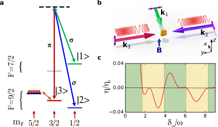
Figure 1: Scheme for realizing driven degenerate Fermi gases with modulated 2D SOC. (a) Energy level diagram of Fermi gases ⁴⁰K. Three hyperfine spin states are coupled with the electronic excited states through three Raman lasers. The atoms are initially prepared in the free reservoir spin state $|9/2,5/2\rangle$. (b) Configuration of three Raman lasers in the $xy$ plane. The detunings of the Raman lasers 2 and 3 are modulated as $\delta_{2(0)}+\delta_{m}\cos(\omega t)$ and $\delta_{3(0)}+\delta_{m}\cos(\omega t+\phi_{0})$. (c) Plot of the product of the effective Raman coupling strengths $\eta=\Omega_{12}^{\prime}\Omega_{13}^{\prime}\Omega_{23}^{\prime}$ (scaled by $\eta_{0}=\Omega_{12}\Omega_{13}\Omega_{23}$) as a function of the modulation parameter $\delta_{m}/\omega$. The background colors indicate the sign of $\eta$ which determines the position of the Dirac point. The relative phase $\phi_{0}=\pi/2$.

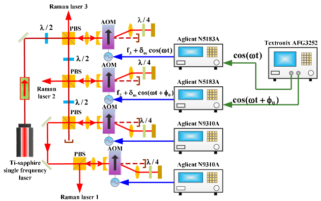
Figure 6: Schematic of generating the Raman lasers. $\lambda/2$: half wave plate; $\lambda/4$: quarter wave plate; PBS: Polarized beam splitter; AOM: acousto-optic modulator.

The experimental setup for generating 2D SOC is the same as that in our previous experiment Huang15 (see Methods). As shown in Fig. 6(a), three hyperfine spin states of the ⁴⁰K Fermi gas are coupled to the electronic excited states by three far-detuned Raman lasers, with the corresponding two-photon Raman coupling strengths between hyperfine states $|j\rangle$ and $|j^{\prime}\rangle$ denoted by $\Omega_{jj^{\prime}}$. The three Raman lasers propagate in the $x$-$y$ plane (Fig. 6(b)), thus the motion of the atoms along $z$ direction is decoupled from the internal degrees of freedom.

In experiment, the two-photon Raman detunings are modulated as $\delta_{2}=\delta_{2(0)}+\delta_{m}\cos(\omega t)$ and $\delta_{3}=\delta_{3(0)}+\delta_{m}\cos(\omega t+\phi_{0})$ by varying the frequencies of the Raman lasers 2 and 3 (see supplementary information supp ). Here, $\phi_{0}$ is the initial relative phase between the two modulations, which could be tuned arbitrarily in experiment. With a high modulation frequency $\omega=2\pi\times 100$ kHz which is much larger than the other relevant energy scales, the system can be described by an effective static Floquet Hamiltonian (see Eq. (1) in Methods), which is the same as that of the unmodulated system with the Raman coupling strengths $\Omega_{jj^{\prime}}$ replaced by $\Omega_{12}^{\prime}=\Omega_{12}J_{0}\left(\delta_{m}/\omega\right)$, $\Omega_{13}^{\prime}=\Omega_{13}J_{0}\left(\delta_{m}/\omega\right)$, and $\Omega_{23}^{\prime}=\Omega_{23}J_{0}\left(2\delta_{m}\sin(\phi_{0}/2)/\omega\right)$ supp . Here $J_{0}(x)$ is the $0$-th order Bessel function. The effective $3\times 3$ static Floquet Hamiltonian (1) has three dressed bands, and the position of the Dirac point is determined by the sign of the quantity $\eta=\Omega_{12}^{\prime}\Omega_{13}^{\prime}\Omega_{23}^{\prime}$. The Dirac point emerges at the crossing of the lower (upper) two bands for negative (positive) $\eta$ Huang15 . By varying the modulating amplitude $\delta_{m}$ and relative phase $\phi_{0}$, we can manipulate $\eta$ (see Fig. 6(c)) and thus alter the topology of the Floquet band structure. For the measurement, we use momentum-resolved spin injection rf spectroscopy to study the energy-momentum dispersions of the dressed states, in which the atoms are driven from a free spin-polarized state (initial state) into the SOC dressed ones (finial states).

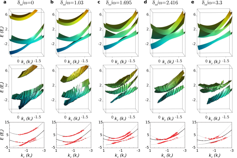
Figure 2: Observation of Floquet band topological change. The upper and middle panels represent theoretically calculated and experimentally measured 2D Floquet band dispersions, respectively. The lower panel represents the corresponding 1D dispersions along $k_{x}=0.05k_{r}$ for (a)-(d) and $k_{x}=-0.7k_{r}$ for (e) where the greyness of the lines indicates the population of the final state $\left|3\right\rangle$. The modulation amplitudes of the Raman detunings are (a) $\delta_{m}/\omega=0$, (b) $1.03$, (c) $1.695$, (d) $2.416$, and (e) $3.3$. Other parameters are $\Omega_{12}=5.46E_{r}$, $\Omega_{13}=4.62E_{r}$, $\Omega_{23}=-4.2E_{r}$, $\delta_{2(0)}=-2.47E_{r}$, and $\delta_{3(0)}=0.93E_{r}$. The relative phase is $\phi_{0}=\pi/2$.

Observation of topology change of Floquet band dispersions: The wavelengths of the Raman lasers are tuned to 768.85 nm between the $D_{1}$ line and $D_{2}$ line, making $\eta=-1$ for the Raman coupling strengths in the absence of the modulation $\delta_{m}=0$. Therefore, the two lower energy bands touch at a Dirac point which is observed in experiment as shown in Fig. 2(a) with the three band dispersions measured by spin-injection rf spectroscopy. The band dispersions are also determined theoretically by calculating the eigenenergy spectrum of the effective static Floquet Hamiltonian (1) and compared with the experimental results.

We first consider the periodic modulations with the relative phase $\phi_{0}=\pi/2$. By increasing $\delta_{m}/\omega$, the three effective Raman coupling strengths decrease, and the Dirac point moves in the momentum space, but still within the lowest two bands for a small $\delta_{m}/\omega$ (see Fig. 2(b)). When $\delta_{m}/\omega\approx 1.7$, $J_{0}(\sqrt{2}\delta_{m}/\omega)=0$ and thus $\Omega_{23}^{\prime}=0$. The two spin states $|2\rangle$ and $|3\rangle$ decouple and the Dirac point moves to infinity, showing three Floquet bands which are gapped everywhere (see Fig. 2(c)). When $\delta_{m}/\omega$ is slightly larger than $1.7$, the Dirac point re-appears at the crossing of the two upper bands because $\Omega_{23}^{\prime}$ changes sign and becomes positive. When $\delta_{m}/\omega\approx 2.4$, $J_{0}(\delta_{m}/\omega)=0$ and thus $\Omega_{12}^{\prime}=\Omega_{13}^{\prime}=0$, the two spin states $|2\rangle$ and $|3\rangle$ are coupled by an effective 1D SOC which does not exhibit a Dirac point. For our experimental parameters, the uncoupled free particle dispersion band for spin state $|1\rangle$ intersects with the upper branch of the 1D SOC (Fig. 2(d)), where a small gap between these two dispersions is opened due to the finite driving frequency $\omega$. By further increasing $\delta_{m}/\omega$, $\Omega_{12}^{\prime}$ and $\Omega_{13}^{\prime}$ change sign simultaneously and thus the Dirac point remains staying at the same crossing of the two upper dressed bands (see Fig. 2(e)). Now the upper band initially without topological properties becomes topological.

We denote $\mathbf{k}_{0}=(k_{x}^{0},k_{y}^{0})$ as the original position of the Dirac point in momentum space in the absence of modulation. In the presence of modulation, the position of the Dirac point is shifted to a different place and there is an energy separation at $\mathbf{k}_{0}$ between the two crossed bands. We characterize the three band dispersions by measuring the energy separations between the three dressed bands at the position of $\mathbf{k}_{0}$. In Fig. 3(a), we plot these energy separations as a function of the modulation parameter $\delta_{m}/\omega$. With the increase of $\delta_{m}/\omega$, the three effective Raman coupling strengths are decreased, the energy separation between the lower two bands at $\mathbf{k}_{0}$ is increased (blue line in Fig. 3(a)), while the separation between the upper two bands is decreased (red line in Fig. 3(a)). The good agreement between experiment and theory demonstrate the expected modulation of the Floquet band dispersion.

In the presence of modulation, the current position of the Dirac point $\mathbf{k=}\left(k_{x},k_{y}\right)$ is different from $\mathbf{k}_{0}$. For different values of $\delta_{m}/\omega$, it can be computed theoretically from the effective static Floquet Hamiltonian (1). In Fig. 3(b), we show the trajectory of the current Dirac point as a function of the modulation parameter $\delta_{m}/\omega$, together with the experimental measured positions for three values of $\delta_{m}/\omega$ shown in Fig. 2. Across the points $\delta_{m}/\omega=z_{n,0}/\sqrt{2}=1.7,3.9,6.1,8.3,\ldots$, the Dirac point moves to infinity (Fig. 2(c)) and then reappears at the crossing of the other two dressed bands (Fig. 2(e)). Here $z_{n,0}$ are the zeros of the Bessel function $J_{0}(z_{n,0})=0$. On the contrary, at the two sides of $\delta_{m}/\omega=2.4,5.5,8.65,11.8,\ldots$, two of the effective Raman couplings change sign simultaneously and the position of the Dirac point does not change. Such observed move of the Dirac point between lower and upper two bands with increasing $\delta_{m}/\omega$ showcases the topology change of Floquet band structure of driven Fermi gases.

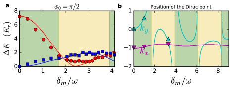
Figure 3: Characterization of the change of the Floquet band structure. (a) Energy separations between three energy bands at $\mathbf{k}_{0}$, the position of the Dirac point in the absence of modulation. The symbols and solid lines correspond to experimental and theoretical results, respectively. (b) Change of the position of the Dirac point as a function of the modulation parameter $\delta_{m}/\omega$. The magenta and cyan lines correspond to theoretical plot of $k_{x}$ and $k_{y}$ of the Dirac point. The symbols correspond to the positions of the measured Dirac point for the three $\delta_{m}/\omega=0$, $1.03$, $3.3$. Note that the Dirac point goes to infinity for $\delta_{m}/\omega=1.7$, as observed in Fig. 2(c). All other parameters are the same as Fig. 2. The background colors in both panels indicate whether the Dirac point exhibits at the crossing of two lower (green) or higher (yellow) bands.

Observation of Floquet sidebands: Periodic driving not only modifies the band structure drastically, but also induces Floquet sidebands. Due to the absorption and emission of integer times of energy $\hbar\omega$, the energy dispersion of the Floquet system repeats itself periodically in the energy domain. Although the sidebands are not easy to be identified in periodically driven bosonic systems, the modulated Fermi gas provides an ideal platform to map out the sidebands using spin injection rf spectroscopy. Fig. 4(a) shows the measured $n=+1$ and $n=-1$ sidebands. According to Floquet theory, the sideband energy dispersions should be a simple copy of $n=0$ dressed energy bands. Here one dressed energy band in $n=+1$ (or $n=-1$) sideband is shown in Fig. 4(a). To test the Floquet theory, we also measure the energy separation of the dressed states at the position of the original Dirac point $\mathbf{k}_{0}$ by including the $n=+1$ and $n=-1$ sidebands as a function of the modulation parameter $\delta_{m}/\omega$. They agree with the theoretical calculation very well as shown in Fig. 4(b). The energy separation between the sidebands and the original bands is around $\sim\hbar\omega=h\times 100$ kHz, the same as the driving frequency.

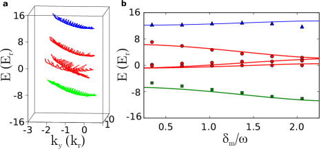
Figure 4: Observation of Floquet sidebands. (a) Plot of the measured energy bands by rf spin-injection spectroscopy with $\delta_{m}/\omega=1.03$. (b) Values of the quasi-energies at $\mathbf{k}_{0}$ as a function of $\delta_{m}/\omega$. The solid lines are the theoretical plots and the symbols are the experimental data. The other parameters are the same as those in Fig. 2.

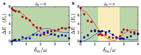
Figure 5: Effect of initial relative phase $\phi_{0}$. The parameters and labels are the same as Fig. 3(a) except that $\phi_{0}=0$ for (a) and $\phi_{0}=\pi$ for (b), respectively.

Effects of relative phase: In the presence of multiple modulations of the system parameters, the relative phase between these modulations plays a key role in the driven dynamics and the energy dispersions of corresponding effective Hamiltonian are usually very different. A prominent example is the comparison between circular and linear drivings of two components of a gauge field where the former one breaks the time reversal symmetry and may lead to the appearance of fascinating topological states while the latter one does not Wang2013 ; Jotzu2014 . Here the relative phase $\phi_{0}$ between the modulation of the two detunings can dramatically change $\Omega_{23}^{\prime}=J_{0}\left(2\delta_{m}\sin(\phi_{0}/2)/\omega\right)$ and thus affect the sign of $\eta$ and the position of the Dirac point. In Fig. 5, we plot the band separations at the original Dirac point $\mathbf{k}_{0}$, similar as Fig. 3(a), but with $\phi_{0}=0$ and $\phi_{0}=\pi$, respectively. When $\phi_{0}=0$, the Raman coupling $\Omega_{23}^{\prime}$ does not change sign during the modulation. The simultaneous change of the other two Raman coupling strengths does not reverse the sign of the parameter $\eta=\Omega_{12}^{\prime}\Omega_{13}^{\prime}\Omega_{23}^{\prime}$, therefore the Dirac point always exhibits at the lower two bands (Fig. 5(a)). However, similar to the case of $\phi_{0}=\pi/2$, $\eta$ changes sign for $\phi_{0}=\pi$, thus the Dirac point moves from the lower two bands to the upper two bands and vice versa (Fig. 5(b)).

Discussions

The motion of atoms along the $z$ direction is decoupled from that in the $xy$ plane, therefore the rf spectroscopy only detects the band dispersion in the $xy$ plane although the Fermi gas can be 3D. For a 2D (or a fixed $k_{z}$ plane in 3D) Fermi gas, a topological band gap at the Dirac point can be opened by varying the polarizations of the Raman lasers, which induces an imaginary part for the Raman coupling strength that corresponds to an effective perpendicular Zeeman field. For example, in the recent experiment Meng15 , an imaginary term $i\Gamma$ has been generated for the Raman coupling $\Omega_{12}$. The exhibited energy gap $\Delta$ at the position of the original Dirac point is found to be proportional to $\Gamma$ and the Chern number of the two bands are given by $\pm\text{sgn}(\Gamma\Omega_{13}\Omega_{23})$. In the presence of the same modulations that we explored, the real and imaginary parts of the Raman coupling $\Omega_{12}$ change sign simultaneously. Consequently, the Chern number of the two gapped bands are given by $\pm\text{sgn}(\eta)$ ($\mp\text{sgn}(\eta)$) if $\Gamma$ is of the same (opposite) sign with $\Omega_{12}$ before the modulations are applied. This provides a useful guide to detect the topological properties of the driven energy bands in the presence of an energy gap. Such topological band gaps support the existence of exotic Majorana fermions in 2D and Weyl fermions in 3D in the presence of pairing interactions, while the periodic driving provides a knob of tuning topological band regions, yielding Floquet Majorana or Weyl fermions.

In conclusion, we have experimentally directly observed the topology change of the Floquet band structure in a periodically driven quantum system using spin-injection rf spectroscopy. Our model system, periodically driven Fermi gases with 2D SOC, provides an ideal platform for testing and understanding rich Floquet physics and band engineering novel exotic quantum materials.

Methods

Experimental setup: The three spin states are selected within the $4^{2}S_{1/2}$ ground electronic manifold with $|1\rangle=|F=7/2,m_{F}=1/2\rangle$, $|2\rangle=|9/2,1/2\rangle$ and $|3\rangle=|9/2,3/2\rangle$, where $(F,m_{F})$ are the quantum numbers for hyperfine spin states. The experiment starts with a Fermi gas of $N=2\times 10^{6}$ ⁴⁰K atoms in a crossed 1064 nm optical dipole trap at $T/T_{F}\approx 0.3$, where $T_{F}$ is the Fermi temperature defined by $T_{F}=(6N)^{1/3}\hbar\overline{\omega}/k_{B}$ with $\bar{\omega}\simeq 2\pi\times 80$ Hz labels the geometric trapping frequency. The fermionic atoms are transferred into $|9/2,5/2\rangle$ as the initial state via a rapid adiabatic passage induced by a rf field at $19.6$ G. Then a homogeneous bias magnetic field along the $z$ axis (gravity direction) is ramped to $B_{0}=121.4$ G by a pair of coils operating in the Helmholtz configuration, splitting the $|3\rangle$ and $|2\rangle$ Zeeman states by $\sim$38.7 MHz and the $|1\rangle$ and $|2\rangle$ states by 1,293 MHz. The large Zeeman splitting would isolate these three hyperfine spin states from other ones in the Raman transitions. We choose the one-photon recoil momentum $\hbar q_{r}$ and the recoil energy $E_{r}=\hbar^{2}q_{r}^{2}/2m=h\times 8.45$ kHz as the natural momentum and energy units. Here $q_{r}=2\pi/\lambda$ and $\lambda$ is the wavelength of the Raman lasers. Using the acoustic-optic modulators (AOM), the frequencies of the Raman lasers 2 and 3 are modulated as $f_{2(0)}+\delta_{m2}\cos(\omega t)$ and $f_{3(0)}+\delta_{m3}\cos(\omega t+\phi_{0})$, respectively, yielding the detuning modulations discussed above (see supplementary information supp ).

Effective Floquet Hamiltonian: With the high-frequency modulation of the Raman detunings, the motion of atoms in the $xy$ plane can be described by an effective static Floquet Hamiltonian

$$H_{xy}^{eff}=\sum_{j=1}^{3}\left(\frac{\hbar^{2}(\mathbf{k}-\mathbf{q}_{j})^{2}}{2m}+\delta_{j(0)}\right)|j\rangle\langle j|-\sum_{j^{\prime}\neq j}\frac{\Omega_{jj^{\prime}}^{\prime}}{2}|j\rangle\langle j^{\prime}|$$ (1)

with the modified Raman coupling strengths $\Omega_{jj^{\prime}}^{\prime}$ due to the fast modulation. Here, $\hbar\mathbf{k}=(\hbar k_{x},\hbar k_{y})$ denotes the momentum of atoms projected on the $x-y$ plane, $\delta_{2(0)}$ ($\delta_{3(0)}$) corresponds to the original two-photon Raman detuning between Raman lasers $1$ and $2$ ($1$ and $3$) without the fast modulation (i.e., $\delta_{1(0)}$ is chosen as 0). The wave vectors of three lasers $\mathbf{q}_{1}=-q_{r}\hat{e}_{x}$, $\mathbf{q}_{2}=q_{r}\hat{e}_{y}$ and $\mathbf{q}_{3}=-q_{r}\hat{e}_{y}$.

Spin-injection spectroscopy: The Raman lasers are derived from a continuous-wave Ti-sapphire single frequency laser with the wavelength $\lambda=768.85$ nm which are ramped up linearly from zero to their final intensity in 60 ms. Subsequently, a Gaussian shape pulse with 450 $\mu s$ of the rf field is applied to drive atoms from $|9/2,5/2\rangle$ to the final empty SOC state. Since the spin state $|9/2,5/2\rangle$ is coupled to the state $|3\rangle$ via rf, spin injection rf spectroscopy will measure the weight of the $|3\rangle$ state and obtain the energy dispersions with 2D SOC. At last, the Raman lasers, the optical trap and the magnetic field are switched off abruptly, and atoms freely expand for 12 ms in a magnetic field gradient applied along the $x$ axis. Absorption image are taken along the $z$ direction. By counting the number of atoms in state $|3\rangle$ as a function of the momentum and the rf frequency from the absorption image, the energy band structure and the position of the Dirac point can be determined.

Acknowledgements: Useful discussions with L. Jiang are acknowledged. This research is supported by the MOST (Grant No. 2016YFA0301600), NSFC (Grant No. 11234008, 11361161002, 11222430). C.Q. and C.Z. are supported by by ARO (W911NF-17-1-0128), AFOSR (FA9550-16-1-0387), and NSF (PHY-1505496).

Author contributions: L.H., P.P., D.L., Z.M., L.C., P.W., and J.Z. performed experiments. C.Q., C.Z. and J.Z. developed the theory. C.Q., C.Z., and J.Z. contributed to the theoretical modelling and explanation of the experimental data. C.Q., C.Z. and J.Z. wrote the paper. All authors discussed the results and commented on the manuscript. J.Z. supervised the project.

Competing financial interests

The authors declare no competing financial interests.

Supplementary Information for “Observation of Floquet band topology change in driven ultracold Fermi gases”

I Theoretical modelling

The three Raman lasers propagate in the x-y plane, thus the motion of the atoms along the z direction is decoupled from the internal degrees of freedom. After the adiabatic elimination of the excited states, the Hamiltonian for atoms can be written as $H=\hbar^{2}k_{z}^{2}/(2m)+H_{xy}$ with

$$H_{xy}=\sum_{j=1}^{3}\left(\frac{\hbar^{2}(\mathbf{k}-\mathbf{q}_{j})^{2}}{2m}+\delta_{j}\right)|j\rangle\langle j|-\sum_{j^{\prime}\neq j}\frac{\Omega_{jj^{\prime}}}{2}|j\rangle\langle j^{\prime}|.$$ (2)

Here, $\hbar\mathbf{k}=(\hbar k_{x},\hbar k_{y})$ denotes the momentum of atoms projected on the $x-y$ plane, $\delta_{1}$ is set as zero (the energy reference) for simplification and $\delta_{2}$ ($\delta_{3}$) corresponds to the two-photon Raman detuning between Raman lasers $1$ and $2$ ($1$ and $3$). The wavevectors of the three lasers are $\mathbf{q}_{j}$ with their magnitudes given by $q_{r}=2\pi/\lambda$ where $\lambda$ is the wavelength of the lasers. For the experimental configuration shown in Fig.1(b) of the main text, the three vectors are given by $\mathbf{q}_{1}=-q_{r}\hat{e}_{x}$, $\mathbf{q}_{2}=q_{r}\hat{e}_{y}$ and $\mathbf{q}_{3}=-q_{r}\hat{e}_{y}$. The two-photon Raman coupling strength between the between hyperfine states $j$ and $j^{\prime}$ is denoted by $\Omega_{jj^{\prime}}$ which is a real number.

The Dirac point exhibited by the Hamiltonian Eq. (2) is robust in the sense that it moves in momentum space without gap opening as long as the three Raman coupling strengths $\Omega_{jj^{\prime}}$ are real. The position of the Dirac point can be manipulated by changing the magnitude or the sign of the Raman coupling. Particularly, the Dirac point appears at the crossing of the two lowest (highest) dressed bands if $\Omega_{12}\Omega_{13}\Omega_{23}<0$ ($>0$). Below, we show that the periodic modulation of the Raman detunings provides another powerful way for the manipulation of the Dirac point and consequently alters the topology of the band structure.

Using the acoustic-optic modulators (AOM), the frequencies of the Raman lasers 2 and 3 are modulated as $f_{2(0)}+\delta_{m2}\cos(\omega t)$ and $f_{3(0)}+\delta_{m3}\cos(\omega t+\phi_{0})$, respectively (see below section B). Consequently, the two-photon Raman detunings become $\delta_{2}=\delta_{2(0)}+\delta_{m2}\cos(\omega t)$ and $\delta_{3}=\delta_{3(0)}+\delta_{m3}\cos(\omega t+\phi_{0})$ where $\phi_{0}$ is the initial relative phase between the two modulations which could be tuned arbitrarily in experiment. The overall phase of two modulations, which amounts to a different launching time of the driving and may play a crucial role for the micromotion of the atoms, is not important for effective model description. However, the relative phase $\phi_{0}$ between the two modulations always appear in the effective Hamiltonian and could change the band structure dramatically.

The modulation frequency $\omega=2\pi/T=2\pi\times 100\text{ kHz}=\text{11.8}E_{r}$ is chosen to be much larger than other energy scales in Eq. (2). For such a high-frequency driving, the system can be described by the following time-independent effective Hamiltonian ($\hbar=1$)

$$H_{xy}^{\text{eff}}=\left(\begin{array}[]{ccc}\frac{(\mathbf{k}-\mathbf{q}_{1})^{2}}{2m}&-\frac{\Omega_{12}^{\prime}}{2}&-\frac{\Omega_{13}^{\prime}}{2}\\ -\frac{\Omega_{12}^{\prime}}{2}&\frac{(\mathbf{k}-\mathbf{q}_{2})^{2}}{2m}+\delta_{2(0)}&-\frac{\Omega_{23}^{\prime}}{2}\\ -\frac{\Omega_{13}^{\prime}}{2}&-\frac{\Omega_{23}^{\prime}}{2}&\frac{(\mathbf{k}-\mathbf{q}_{3})^{2}}{2m}+\delta_{3(0)}\end{array}\right),$$ (3)

with the three effective Raman coupling strengths $\Omega_{jj^{\prime}}^{\prime}$ are given by

$$\Omega_{12}^{\prime} = \Omega_{12}\times\frac{1}{T}\int_{0}^{T}e^{-i\delta_{m2}\sin(\omega t)/\omega}dt=\Omega_{12}J_{0}\left(\frac{\delta_{m2}}{\omega}\right),$$

$$\Omega_{13}^{\prime} = \Omega_{13}\times\frac{1}{T}\int_{0}^{T}e^{-i\delta_{m3}\sin(\omega t+\phi_{0})/\omega}dt=\Omega_{13}J_{0}\left(\frac{\delta_{m3}}{\omega}\right),$$

$$\Omega_{23}^{\prime} = \Omega_{23}\times\frac{1}{T}\int_{0}^{T}e^{i\delta_{m2}\sin(\omega t)/\omega}e^{-i\delta_{m3}\sin(\omega t+\phi_{0})/\omega}dt$$ (4)

$$= \Omega_{23}\bigg{[}J_{0}\left(\frac{\delta_{m2}}{\omega}\right)J_{0}\left(\frac{\delta_{m3}}{\omega}\right)+2\sum_{n=1}^{\infty}J_{n}\left(\frac{\delta_{m2}}{\omega}\right)\times$$

$$J_{n}\left(\frac{\delta_{m3}}{\omega}\right)\cos(n\phi_{0})\bigg{]}$$

where $J_{n}(x)$ is the $n$-th order Bessel function of the first kind. Note that the three effective Raman coupling strengths are still real and thus the Dirac point is protected under the periodic modulation of the detunings. In this work, we will consider the same modulation amplitudes for the two detunings, i.e., $\delta_{m2}=\delta_{m3}=\delta_{m}$. In this situation, the effective Raman coupling strength $\Omega_{23}^{\prime}$ can be simplified to

$$\Omega_{23}^{\prime} = \Omega_{23}\times\frac{1}{T}\int_{0}^{T}e^{-i2\delta_{m}\cos(\omega t+\phi_{0}/2)\sin(\phi_{0}/2)/\omega}dt$$ (5)

$$= J_{0}\left(\frac{2\delta_{m}}{\omega}\sin(\phi_{0}/2)\right).$$

Although the effective Raman couplings remain real numbers, because of the nature of the Bessel functions, the signs of the effective Raman coupling strengths $\Omega_{jj^{\prime}}^{\prime}$ and thus their product $\eta=\Omega_{12}^{\prime}\Omega_{23}^{\prime}\Omega_{13}^{\prime}$ could be reversed in the modulation (see Fig.1(c) of the main text). As a result, the Dirac point may appear at the crossing of different dressed bands depending on the laser parameters.

Below we show the derivation of the static effective Hamiltonian (3).

I.1 First method

The time-dependent Hamiltonian is given by (we have taken $E_{r}={\hbar^{2}k_{r}^{2}}/{2m}$ and $\hbar k_{r}$ as the units for the energy and momentum),

$$H=\left(\begin{array}[]{lll}(\mathbf{k}-\mathbf{q}_{1})^{2}&-\frac{\Omega_{12}}{2}&-\frac{\Omega_{13}}{2}\\ -\frac{\Omega_{12}}{2}&(\mathbf{k}-\mathbf{q}_{2})^{2}+\delta_{2}(t)&-\frac{\Omega_{23}}{2}\\ -\frac{\Omega_{13}}{2}&-\frac{\Omega_{23}}{2}&(\mathbf{k}-\mathbf{q}_{3})^{2}+\delta_{3}(t)\end{array}\right).$$ (6)

The two detunings are modulated in the following way

$$\delta_{2} = \delta_{2(0)}+\delta_{m2}\cos(\omega t+\alpha),$$ (7)

$$\delta_{3} = \delta_{3(0)}+\delta_{m3}\cos(\omega t+\alpha+\phi_{0}),$$ (8)

where $\alpha$ is the initial phase of the modulation and $\phi_{0}$ is the relative phase between the two modulations.

To eliminate the time-dependence, one can apply a time-dependent unitary transformation of the following form

$$U=\left(\begin{array}[]{ccc}1&0&0\\ 0&e^{-i\frac{\delta_{m2}}{\omega}\sin(\omega t+\alpha)}&0\\ 0&0&e^{-i\frac{\delta_{m3}}{\omega}\sin(\omega t+\alpha+\phi_{0})}\end{array}\right).$$ (9)

The wave function is then transformed as $\tilde{\Psi}=U^{-1}\Psi$, i.e.,

$$\tilde{\Psi}=\left(\begin{array}[]{c}\tilde{\Psi}_{1}\\ \tilde{\Psi}_{2}\\ \tilde{\Psi}_{3}\end{array}\right)=\left(\begin{array}[]{c}\Psi_{1}\\ e^{i\frac{\delta_{m2}}{\omega}\sin(\omega t+\alpha)}\Psi_{2}\\ e^{i\frac{\delta_{m3}}{\omega}\sin(\omega t+\alpha+\phi_{0})}\Psi_{3}\end{array}\right)$$ (10)

The Hamiltonian is transformed as $\tilde{H}=U^{-1}HU-iU^{-1}\frac{\partial U}{\partial t}$, i.e.,

$$\tilde{H}=\left(\begin{array}[]{ccc}(\mathbf{k}-\mathbf{q}_{1})^{2}&-\frac{\Omega_{12}}{2}e^{-i\frac{\delta_{m2}}{\omega}\sin(\omega t+\alpha)}&-\frac{\Omega_{13}}{2}e^{-i\frac{\delta_{m3}}{\omega}\sin(\omega t+\alpha+\phi_{0})}\\ -\frac{\Omega_{12}}{2}e^{i\frac{\delta_{m2}}{\omega}\sin(\omega t+\alpha)}&(\mathbf{k}-\mathbf{q}_{2})^{2}+\delta_{2(0)}&-\frac{\Omega_{23}}{2}e^{i\frac{\delta_{m2}}{\omega}\sin(\omega t+\alpha)}e^{-i\frac{\delta_{m3}}{\omega}\sin(\omega t+\alpha+\phi_{0})}\\ -\frac{\Omega_{13}}{2}e^{i\frac{\delta_{m3}}{\omega}\sin(\omega t+\alpha+\phi_{0})}&-\frac{\Omega_{23}}{2}e^{-i\frac{\delta_{m2}}{\omega}\sin(\omega t+\alpha)}e^{i\frac{\delta_{m3}}{\omega}\sin(\omega t+\alpha+\phi_{0})}&(\mathbf{k}-\mathbf{q}_{3})^{2}+\delta_{3(0)}\end{array}\right).$$

The effective Hamiltonian is defined as the time-average of $\tilde{H}$ in one period

$$H_{eff}=\frac{\omega}{2\pi}\int_{0}^{2\pi/\omega}\tilde{H}(t)dt.$$ (11)

Therefore the diagonal parts do not change while the non-diagonal parts will be averaged out, yielding effective Raman couplings

$$\Omega_{12}^{\prime} = \Omega_{12}\frac{\omega}{2\pi}\int_{0}^{2\pi/\omega}e^{-i\frac{\delta_{m2}}{\omega}\sin(\omega t+\alpha)}dt=\frac{\Omega_{12}}{2\pi}\int_{0}^{2\pi}e^{-i\frac{\delta_{m2}}{\omega}\sin(\tau+\alpha)}d\tau=\Omega_{12}J_{0}\left(\frac{\delta_{m2}}{\omega}\right),$$ (12)

$$\Omega_{13}^{\prime} = \Omega_{13}\frac{\omega}{2\pi}\int_{0}^{2\pi/\omega}e^{-i\frac{\delta_{m3}}{\omega}\sin(\omega t+\alpha+\phi_{0})}dt=\frac{\Omega_{13}}{2\pi}\int_{0}^{2\pi}e^{-i\frac{\delta_{m3}}{\omega}\cos(\tau+\alpha+\phi_{0})}d\tau=\Omega_{13}J_{0}\left(\frac{\delta_{m3}}{\omega}\right),$$ (13)

$$\Omega_{23}^{\prime} = \Omega_{23}\frac{\omega}{2\pi}\int_{0}^{2\pi/\omega}e^{i\frac{\delta_{m2}}{\omega}\sin(\omega t+\alpha)}e^{-i\frac{\delta_{m3}}{\hbar}\sin(\omega t+\alpha+\phi_{0})}dt$$ (14)

$$= \Omega_{23}\bigg{[}J_{0}\left(\frac{\delta_{m2}}{\omega}\right)J_{0}\left(\frac{\delta_{m3}}{\omega}\right)+2\sum_{n=1}^{\infty}J_{n}\left(\frac{\delta_{m2}}{\omega}\right)\times J_{n}\left(\frac{\delta_{m3}}{\omega}\right)\cos(n\phi_{0})\bigg{]}.$$

If $\delta_{m2}=\delta_{m3}$, then $\Omega_{23}^{\prime}$ can be simplified to

$$\Omega_{23}^{\prime} = \Omega_{23}\frac{1}{2\pi}\int_{0}^{2\pi}e^{i\frac{\delta_{m}}{\omega}[\sin(\tau+\alpha)-\sin(\tau+\alpha+\phi_{0})]}d\tau=\frac{\Omega_{23}}{2\pi}\int_{0}^{2\pi}e^{-i\frac{2\delta_{m}}{\omega}\sin\frac{\phi_{0}}{2}\cos(\tau+\alpha+\frac{\phi_{0}}{2})}d\tau$$ (15)

$$= \Omega_{23}J_{0}\left(\frac{2\delta_{m}}{\omega}\sin(\phi_{0}/2)\right).$$

Particularly, we find (i) $\Omega_{23}^{\prime}=\Omega_{23}$ for $\phi_{0}=0$; (ii) $\Omega_{23}^{\prime}=\Omega_{23}J_{0}(\sqrt{2}\delta_{m}/\omega)$ for $\phi_{0}=\pi/2$; (iii) $\Omega_{23}^{\prime}=\Omega_{23}J_{0}(2\delta_{m}/\omega)$ for $\phi_{0}=\pi$.

I.2 Second method

The effective Hamiltonian can also be derived from the Goldman-Dalibard method Goldman2014 . The equation is

$$H_{eff}=H_{0}+\frac{1}{\omega}\sum_{j=1}^{\infty}\frac{1}{j}[V^{(j)},V^{(-j)}]+\frac{1}{2\omega^{2}}\sum_{j}^{\infty}\frac{1}{j^{2}}\left([[V^{(j)},H_{0}],V^{(-j)}]+[[V^{(-j)},H_{0}],V^{(j)}]\right)+\mathcal{O}\left(\frac{1}{\omega^{3}}\right).$$ (16)

This methods becomes cumbersome for high order terms. But for high frequency limit, we can safely keep the first several terms and find the approximate effective Hamiltonian with good precision.

In the above expression, $H_{0}$ is the time-independent part of the Hamiltonian and

$$V^{(+1)}=\left(\begin{array}[]{ccc}0&0&0\\ 0&\frac{\delta_{m2}}{2}e^{i\alpha}&0\\ 0&0&\frac{\delta_{m3}}{2}e^{i(\alpha+\phi_{0})}\end{array}\right),\qquad V^{(-1)}=\left(\begin{array}[]{ccc}0&0&0\\ 0&\frac{\delta_{m2}}{2}e^{-i\alpha}&0\\ 0&0&\frac{\delta_{m3}}{2}e^{-i(\alpha+\phi_{0})}\end{array}\right)$$ (17)

are positive and negative frequency parts of the periodic driving of $\delta_{2}$ and $\delta_{3}$. Actually, the first order term vanishes and the second term gives the effective Raman couplings

$$\Omega_{12}^{\prime} = \Omega_{12}\left(1-\frac{\delta_{m2}^{2}}{4\omega^{2}}+\ldots\right),$$ (18)

$$\Omega_{13}^{\prime} = \Omega_{13}\left(1-\frac{\delta_{m3}^{2}}{4\omega^{2}}+\ldots\right),$$ (19)

$$\Omega_{23}^{\prime} = \Omega_{23}\left(1-\frac{\delta_{m2}^{2}+\delta_{m3}^{2}-2\delta_{m2}\delta_{m3}\cos\phi_{0}}{4\omega^{2}}+\ldots\right).$$ (20)

If $\delta_{m2}=\delta_{m3}$, then $\Omega_{23}^{\prime}=\Omega_{23}\left[1-\frac{1}{4}\left(\frac{2\delta_{m}}{\omega}\sin\frac{\phi_{0}}{2}\right)^{2}+\ldots\right]$. Using the series expansions for Bessel functions, it is easy to find that the above expressions are the same (up to the order of $1/\omega^{2}$) as that derived using the first method.

The so-called kick operator at time $t$ is given by

$$K(t)=\frac{1}{i\omega}\sum_{j=1}^{\infty}\frac{1}{j}\left(V^{(j)}e^{ij\omega t}-V^{(-j)}e^{-ij\omega t}\right)$$ (21)

For our system, we have

$$K(t)=\left(\begin{array}[]{ccc}0&0&0\\ 0&\frac{\delta_{m2}}{\omega}\sin(\omega t+\alpha)&0\\ 0&0&\frac{\delta_{m3}}{\omega}\sin(\omega t+\alpha+\phi_{0})\end{array}\right),$$ (22)

which is diagonal. Therefore, the time-evolution operator for the original Hamiltonian over a complete driving period takes the form

$$U(t=t_{0}+T,t_{0})=e^{-iTH_{t_{0}}^{F}}=e^{-iK(t=t_{0}+T)}e^{-iTH_{eff}}e^{iK(t_{0})}.$$ (23)

Here, the effective Hamiltonian $H_{eff}$ does not depend on the initial time $t_{0}$. Its eigenvalues, i.e, the quasi-energies, determine the linear phase evolution of the system. One should distinguish the effective Hamitonian from $H_{t_{0}}^{F}$ which contains the information of the micromotion operator $U_{F}(t)=e^{-iK(t)}$. It is easy to realize that $U_{F}(t)$ is just the unitary operator (Eq. (9)) that we have introduced in the previous method.

II Evolution of the chirality of the Dirac point in the modulation

The low-energy effective Hamiltonian near the Dirac point can be written as (see Meng15 )

$$H_{eff}=\epsilon(\mathbf{p})\sigma_{0}+(-\alpha_{y}p_{y}+h_{x})\sigma_{x}+(\beta_{y}p_{y}-\beta_{x}p_{x}+h_{z})\sigma_{z}$$ (24)

where $\alpha_{y}$, $h_{x}$, $\beta_{y}$, $\beta_{x}$, $h_{z}$ are functions of the system parameters $\Omega_{12}$, $\Omega_{23}$, $\Omega_{13}$, $\delta_{2}$, $\delta_{3}$, etc. The Dirac point appears at $p_{y}^{D}=h_{x}/\alpha_{y}$ and $p_{x}^{D}=(\beta_{y}p_{y}^{D}+h_{z})/\beta_{x}$. By shifting the reference frame to this point and redefining the momentum, one simplifies the above Hamiltonian to

$$H_{eff}=\epsilon(\mathbf{p})\sigma_{0}+(-\alpha_{y}p_{y})\sigma_{x}+(\beta_{y}p_{y}-\beta_{x}p_{x})\sigma_{z}+\lambda\sigma_{y}$$ (25)

One finds Xiao2010 that the chirality of the Dirac point is determined by the coefficients $\alpha_{y}$ and $\beta_{x}$. Since $\text{sgn}(\alpha_{y}\beta_{x})=\text{sgn}(\Omega_{13}\Omega_{23})$. Therefore, the chirality reverses sign whenever one of the two Raman coupling $\Omega_{13}$ and $\Omega_{23}$ change sign.

III The configuration of Raman lasers

The Raman lasers are derived from a continuous-wave Ti-sapphire single frequency laser (M Squared lasers, SolsTiS) with the wavelength 768.85 nm as shown in Fig. S1. The Raman laser 1 is sent through the two double-pass acousto-optic modulators (AOM) (3200-124, Crystal Technology, Inc) driven by two signal generators (N9310A, Agilent) and frequency shifted -212.975$\times$4 MHz. The Raman laser 2 and 3 double-pass through two AOM and are frequency-shifted +201.144$\times$2 and +220.531$\times$2 MHz respectively. In order to periodically drive the two-photon Raman detuning, the Raman laser 2 and 3 are frequency modulated respectively with $f_{2(0)}+\delta_{m2}\cos(\omega t)$ and $f_{3(0)}+\delta_{m3}\cos(\omega t+\phi_{0})$, in which a signal generator (AFG3252 Textronix) generates $\cos(\omega t)$ and $\cos(\omega t+\phi_{0})$ signal outputs simultaneously to externally modulate the frequencies of two signal generators (N5183A, Agilent) for Raman lasers 2 and 3. The modulation frequency response of the frequency modulation of the signal generator (N5183A, Agilent) may reach 3 MHz and the maximum deviation is about 10 MHz, which can satisfy the experimental requirement.

References

- (1) Linder, N. H., Refael, G. & Galitski, V. Floquet topological insulator in semiconductor quantum wells, Nat. Phys. 7, 490 (2011).
- (2) Aidelsburger, M., Atala, M., Lohse, M., Barreiro, J. T., Paredes, B. & Bloch, I. Realization of the Hofstadter Hamiltonian with Ultracold Atoms in Optical Lattices, Phys. Rev. Lett. 111, 185301 (2013).
- (3) Miyake, H., Siviloglou, G. A., Kennedy, C. J., Burton, W. C. & Ketterle, W. Realizing the Harper Hamiltonian with Laser-Assisted Tunneling in Optical Lattices, Phys. Rev. Lett. 111, 185302 (2013).
- (4) Rechtsman, M. C., Zeuner, J. M., Plotnik, Y., Lumer, Y., Podolsky, D., Dreisow, F., Nolte, S., Segev, M. & Szameit, A. Photonic Floquet topological insulators, Nature 496, 196 (2013).
- (5) Wang, Y. H., Steinberg, H., Jarillo-Herrero, P. & Gedik, N. Observation of Floquet-Bloch States on the Surface of a Topological Insulator, Science 342, 453 (2013).
- (6) Eckard, A. Atomic quantum gases in periodically driven optical lattices, arXiv:1606.08041
- (7) Jotzu, G., Messer, M., Desbuquois, R., Lebrat, M., Uehlinger, T., Greif, D. & Esslinger, T. Nature 515, 237 (2014).
- (8) Haldane, F. D. M., Model for a Quantum Hall Effect without Landau Levels: Condensed-Matter Realization of the “Parity Anomaly”, Phys. Rev. Lett. 61, 2015 (1988).
- (9) Parker, C. V., Ha, L.-C. & Chin, C. Direct observation of effective ferromagnetic domains of cold atoms in a shaken optical lattice, Nat. Phys. 9, 769 (2013).
- (10) Jiménez-Garzia, K., LeBlanc, L. J., Williams, R. A., Beeler, M. C., Qu, C., Gong, M., Zhang, C. & Spielman, I. B. Tunable Spin-Orbit Coupling via Strong Driving in Ultracold-Atom Systems, Phys. Rev. Lett. 114, 125301 (2015).
- (11) Khamehchi, M. A., Qu, C., Mossman, M. E., Zhang, C. & Engels, P. Spin-momentum coupled Bose-Einstein condensates with lattice band pseudospins, Nat. Commun. 7, 10867 (2016).
- (12) Hasan, M. Z. & Kane, C. L. Colloquium: Topological insulators, Rev. Mod. Phys. 82, 3045 (2010).
- (13) Qi, X.-L. & Zhang, S.-C. Topological insulators and superconductors Rev. Mod. Phys. 83, 1057 (2011).
- (14) Bychkov, Y. A. & Rashba, E. I. Oscillatory effects and the magnetic susceptibility of carriers in inversion layers. J. Phys. C 17, 6039 (1984).
- (15) Dresselhaus, G., Spin-orbit coupling effects in zinc blende structures, Phys. Rev. 100, 580 (1955).
- (16) Lin, Y.-J., Jiménez-García, K. & Spielman, I. B. Spin-orbit-coupled Bose-Einstein condensates. Nature 471, 83-86 (2011).
- (17) Fu, Z., Wang, P., Chai, S., Huang, L. & Zhang, J. Bose- Einstein condensate in a light-induced vector gauge potential using the 1064 nm optical dipole trap lasers. Phys. Rev. A 84, 043609 (2011).
- (18) Zhang, J.-Y. et al. Collective dipole oscillations of a spin-orbit coupled Bose-Einstein condensate. Phys. Rev. Lett. 109, 115301 (2012).
- (19) Qu, C., Hamner, C., Gong, M., Zhang, C. & Engels, P. Observation of Zitterbewegung in a spin-orbit coupled Bose-Einstein condensates. Phys. Rev. A 88, 021604(R) (2013)
- (20) Olson, A. J., Wang, S. -J., Niffenegger, R. J., Li, C. -H., Greene, C. H. & Chen, Y. P. Tunable Laudan-Zener transitions in a spin-orbit-coupled Bose-Einstein condesate. Phys. Rev. A 90, 013616 (2014).
- (21) Wang, P., Yu, Z., Fu, Z., Miao, J., Huang, L., Chai, S., Zhai, H. & Zhang, J. Spin-orbit coupled degenerate Fermi gases. Phys. Rev. Lett. 109, 095301 (2012).
- (22) Cheuk, L. W. et al. Spin-injection spectroscopy of a spin-orbit coupled Fermi gas. Phys. Rev. Lett. 109, 095302 (2012).
- (23) Williams, R. A., Beeler, M. C., LeBlanc, L. J. & Spielman I. B. Raman-induced interactions in a single-component Fermi gas near an s-wave Feshbach resonance. Phys. Rev. Lett. 111, 095301 (2013).
- (24) Burdick, N. Q., Tang, Y. & Lev, B. L. Long-Lived Spin-Orbit-Coupled Degenerate Dipolar Fermi Gas, Phys. Rev. X 6, 031022 (2016).
- (25) Song, B., He, C., Zhang, S., Hajiyev, E., Huang, W., Liu, X.-J. & Jo, G.-B., Spin-orbit-coupled two-electron Fermi gases of ytterbium atoms. Phys. Rev. A 94, 061604(R) (2016).
- (26) Huang, L., Meng, Z., Wang, P., Peng, P., Zhang, S.-L., Chen, L., Li, D., Zhou, Q. & Zhang, J. Experimental realization of a two-dimensional synthetic spin-orbit coupling in ultracold Fermi gases. Nat. Phys. 12, 540 (2016).
- (27) Meng, Z., Huang, L., Peng, P., Li, D., Chen, L., Xu, Y., Zhang, C., Wang, P. & Zhang, J. Experimental observation of topological band gap opening in ultrocold Fermi gases with two-dimensional spin-orbit coupling, Phys. Rev. Lett. 117, 235304 (2016).
- (28) Goldman, N. & Dalibard, J. Periodically Driven Quantum Systems: Effective Hamiltonians and Engineered Gauge Fields, Phys. Rev. X 4, 031027 (2014).
- (29) Eckardt, A. & Anisimovas, E. High-frequency approximation for periodically driven quantum systems from a Floquet-space perspective, New. J. Phys. 17, 093039 (2015).
- (30) Bukov, M., D’Alessio, L. & POlkovnikov, A. Universal High-Frequency Behavior of Periodically Driven Systems: from Dynamical Stabilization to Floquet Engineering, Advances in Physics, 64, 139 (2015).
- (31) Our supplementary materials.
- (32) D. Xiao, M.-C. Chang and Q. Niu, Rev. Mod. Phys. 82, 1959 (2010).