Ontological Multidimensional Data Models and Contextual Data Quality

Abstract.

Data quality assessment and data cleaning are context-dependent activities. Motivated by this observation, we propose the Ontological Multidimensional Data Model (OMD model), which can be used to model and represent contexts as logic-based ontologies. The data under assessment is mapped into the context, for additional analysis, processing, and quality data extraction. The resulting contexts allow for the representation of dimensions, and multidimensional data quality assessment becomes possible. At the core of a multidimensional context we include a generalized multidimensional data model and a Datalog^± ontology with provably good properties in terms of query answering. These main components are used to represent dimension hierarchies, dimensional constraints, dimensional rules, and define predicates for quality data specification. Query answering relies upon and triggers navigation through dimension hierarchies, and becomes the basic tool for the extraction of quality data. The OMD model is interesting per se, beyond applications to data quality. It allows for a logic-based, and computationally tractable representation of multidimensional data, extending previous multidimensional data models with additional expressive power and functionalities.

1. Introduction

Assessing the quality of data and performing data cleaning when the data are not up to the expected standards of quality have been and will continue being common, difficult and costly problems in data management (Batini & Scannapieco, 2006; Eckerson, 2002; Redman, 1998). This is due, among other factors, to the fact that there is no uniform, general definition of quality data. Actually, data quality has several dimensions. Some of them are (Batini & Scannapieco, 2006): (1) Consistency, which refers to the validity and integrity of data representing real-world entities, typically identified with satisfaction of integrity constraints. (2) Currency (or timeliness), which aims to identify the current values of entities represented by tuples in a (possibly stale) database, and to answer queries with the current values. (3) Accuracy, which refers to the closeness of values in a database to the true values for the entities that the data in the database represents; and (4) Completeness, which is characterized in terms of the presence/absence of values. (5) Redundancy, e.g. multiple representations of external entities or of certain aspects thereof. Etc. (Cf. also (Jiang et al., 2008; Fan, 2015; Fan & Geerts, 2012) for more on quality dimensions.)

In this work we consider data quality as referring to the degree to which the data fits or fulfills a form of usage (Batini & Scannapieco, 2006), relating our data quality concerns to the production and the use of data. We will elaborate more on this after the motivating example in this introduction.

Independently from the quality dimension we may consider, data quality assessment and data cleaning are context-dependent activities. This is our starting point, and the one leading our research. In more concrete terms, the quality of data has to be assessed with some form of contextual knowledge; and whatever we do with the data in the direction of data cleaning also depends on contextual knowledge. For example, contextual knowledge can tell us if the data we have is incomplete or inconsistent. In the latter case, the context knowledge is provided by explicit semantic constraints.

In order to address contextual data quality issues, we need a formal model of context. In very general terms, the big picture is as follows. A database can be seen as a logical theory, $\mathcal{T}$, and a context for it, as another logical theory, $\mathcal{T}^{c}$, into which $\mathcal{T}$ is mapped by means of a set, $\mathfrak{m}$, of logical mappings, as shown in Figure 1. The image of $\mathcal{T}$ in $\mathcal{T}^{c}$ is $\mathcal{T}^{\prime}=\mathfrak{m}(\mathcal{T})$, which could be seen as an interpretation of $\mathcal{T}$ in $\mathcal{T}^{c}$. The contextual theory $\mathcal{T}^{c}$ provides extra knowledge about $\mathcal{T}$, as a logical extension of its image $\mathcal{T}^{\prime}$. For example, $\mathcal{T}^{c}$ may contain additional semantic constraints on elements of $\mathcal{T}$ (or their images in $\mathcal{T}^{c}$) or extensions of their definitions. In this way, $\mathcal{T}^{c}$ conveys more semantics or meaning about $\mathcal{T}$, contributing to making more sense of $\mathcal{T}$’s elements. $\mathcal{T}^{c}$ may also contain data and logical rules that can be used for further processing or using knowledge in $\mathcal{T}$. The embedding of $\mathcal{T}$ into $\mathcal{T}^{c}$ can be achieved via predicates in common or, more complex logical formulas.

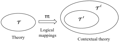
Figure 1. Embedding into a contextual theory

In this work, building upon and considerably extending the framework in (Bertossi et al., 2011a, 2016), context-based data quality assessment, quality data extraction and data cleaning on a relational database $D$ for a relational schema $\mathcal{R}$ are approached by creating a context model where $D$ is the theory $\mathcal{T}$ above (it could be expressed as a logical theory (Reiter, 1984)), the theory $\mathcal{T}^{c}$ is a (logical) ontology $\mathcal{O}^{c}$; and, considering that we are using theories around data, the mappings can be logical mappings as used in virtual data integration (Lenzerini, 2002) or data exchange (Barcelo, 2009). In this work, the mappings turn out to be quite simple: The ontology contains, among other predicates, nicknames for the predicates in $\mathcal{R}$ (i.e. copies of them), so that each predicate $P$ in $\mathcal{R}$ is directly mapped to its copy $P^{\prime}$ in $\mathcal{O}^{c}$.

Once the data in $D$ is mapped into $\mathcal{O}^{c}$, i.e. put in context, the extra elements in it can be used to define alternative versions of $D$, in our case, clean or quality versions, $D^{q}$, of $D$ in terms of data quality. The data quality criteria are imposed within $\mathcal{O}^{c}$. This may determine a class of possible quality versions of $D$, virtual or material. The existence of several quality versions reflects the uncertainty that emerges from not having only quality data in $D$.

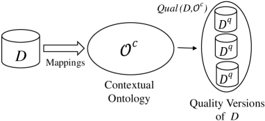
Figure 2. Contextual ontology and quality versions

The whole class, ${\it Qual}(D,\mathcal{O}^{c})$, of quality versions of $D$ determines or characterizes the quality data in $D$, as the data that are certain with respect to ${\it Qual}(D,\mathcal{O}^{c})$. One way to go in this direction consists in keeping only the data that are found in the intersection of all the instances in ${\it Qual}(D,\mathcal{O}^{c})$. A more relaxed alternative consists in considering as quality data those that are obtained as certain answers to queries posed to $D$, but answered through ${\it Qual}(D,\mathcal{O}^{c})$: The query is posed to each of the instances in ${\it Qual}(D,\mathcal{O}^{c})$ (which essentially have the same schema as $D$), but only those answers that are shared by those instances are considered to be certain (Imielinski & Lipski, 1984). These answers become the quality-answers in our setting.

The main question is about the kind of contextual ontologies that are appropriate for our tasks. There are several basic conditions to satisfy. First of all, $\mathcal{O}^{c}$ has to be written in a logical language. As a theory it has to be expressive enough, but not too much so that computational problems, such as (quality) data extraction via queries becomes intractable, if not impossible. It also has to combine well with relational data. And, as we emphasize and exploit in our work, it has to allow for the representation and use of dimensions of data, i.e. conceptual axes along which data are represented and analyzed. They are the basic elements in multidimensional databases and data warehouses (Jensen et al., 2010), where we usually find time, location, product, as three dimensions that give context to numerical data, e.g. sales. Dimensions are almost essential elements of contexts, in general, and crucial if we want to analyze data from different perspectives or points of view. We use dimensions as (possibly partially ordered) hierarchies of categories. For example, the location dimension could have categories, city, province, country, continent, in this hierarchical order of abstraction.

The language of choice for the contextual ontologies will be Datalog^± (Calì et al., 2009). As an extension of Datalog, a declarative query language for relational databases (Ceri et al., 1990), it provides declarative extensions of relational data by means of expressive rules and semantic constraints. Certain classes of Datalog^± programs have non-trivial expressive power and good computational properties at the same time. One of those good classes is that of weakly-sticky Datalog^± (Calì et al., 2012c). Programs in that class allow us to represent a logic-based, relational reconstruction and extension of the Hurtado-Mendelzon multidimensional data model (Hurtado & Mendelzon, 2002; Hurtado et al., 2005), which allows us to bring data dimensions into contexts.

Every contextual ontology $\mathcal{O}^{c}$ contains its multidimensional core ontology, $\mathcal{O}^{M}$, which is written in Datalog^± and represents what we will call the ontological multidimensional data model (OMD model, in short), plus a quality-oriented sub-ontology, $\mathcal{O}^{q}$, containing extra relational data (shown as instance $E$ in Figure 5), Datalog rules, and possibly additional constraints. Both sub-ontologies are application dependent, but $\mathcal{O}^{M}$ follows a relatively fixed format, and contains the dimensional structure and data that extend and supplement the data in the input instance $D$, without any explicit quality concerns in it. The OMD model is interesting per se in that it considerably extends the usual multidimensional data models (more on this later). Ontology $\mathcal{O}^{q}$ contains as main elements definitions of quality predicates that will be used to produce quality versions of the original tables, and to compute quality query answers. Notice that the latter problem becomes a case of ontology-based data access (OBDA), i.e. about indirectly accessing underlying data through queries posed to the interface and elements of an ontology (Poggi et al., 2008).

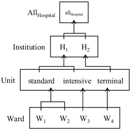
Figure 3. The Hospital dimension

Table 1. ${\it Temperatures}$

	Time	Patient	Value	Nurse
1	12:10-Sep/1/2016	Tom Waits	38.2	Anna
2	11:50-Sep/6/2016	Tom Waits	37.1	Helen
3	12:15-Nov/12/2016	Tom Waits	37.7	Alan
4	12:00-Aug/21/2016	Tom Waits	37.0	Sara
5	11:05-Sep/5/2016	Lou Reed	37.5	Helen
6	12:15-Aug/21/2016	Lou Reed	38.0	Sara

Table 2. ${\it Temperatures}^{q}$

	Time	Patient	Value	Nurse
1	12:15-Nov/12/2016	Tom Waits	37.7	Alan
2	12:00-Aug/21/2016	Tom Waits	37.0	Sara
3	12:15-Aug/21/2016	Lou Reed	38.0	Sara

Example 1.1.

The relational table Temperatures (Table 1) shows body temperatures of patients in an institution. A doctor wants to know “The body temperatures of Tom Waits for August 21 taken around noon with a thermometer of brand $B_{1}$” (as he expected). Possibly a nurse, unaware of this requirement, used a thermometer of brand $B_{2}$, storing the data in Temperatures. In this case, not all the temperature measurements in the table are up to the expected quality. However, table Temperatures alone does not discriminate between intended values (those taken with brand $B_{1}$) and the others.

For assessing the quality of the data or for extracting quality data in/from the table Temperatures according to the doctor’s quality requirement, extra contextual information about the thermometers in use may help. In this case, we may have contextual information in the form of a guideline prescribing that: “Nurses in intensive care unit use thermometers of Brand $B_{1}$”​. We still cannot combine this guideline with the data in the table. However, if we know that nurses work in wards, and those wards are associated to units, then we may be in position to combine the table with the given contextual information. Actually, as shown in Figure 4, the context contains dimensional data, in categorical relations linked to dimensions.

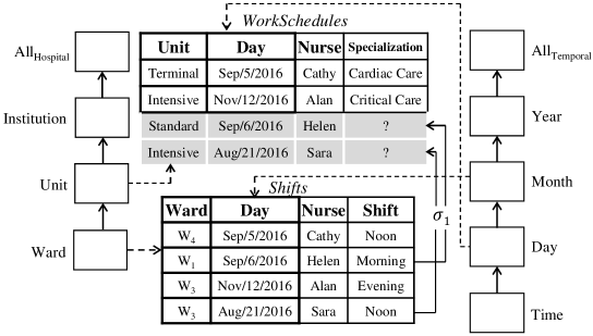
Figure 4. Dimensional data with categorical relations

In it we find two dimensions, $\sf{Hospital}$, on the left-hand side, and $\sf{Temporal}$, on the right-hand side. For example, the $\sf{Hospital}$ dimension’s instance is found in Figure 3. In the middle of Figure 4 we find categorical relations (shown as solid tables and initially excluding the two rows shaded in gray at the bottom of the top table). They are associated to categories in the dimensions.

Now we have all the necessary information to discriminate between quality and non-quality entries in Table 1: Nurses appearing in it are associated to wards, as shown in table Shifts; and the wards are associated to units, as shown in Figure 3. Table WorkSchedules may be incomplete, and new -possibly virtual- entries can be produced for it, showing Helen and Sara working for the Standard and Intensive units, resp. (These correspond to the two (potential) extra, shaded tuples in Figure 4.) This is done by upward navigation and data propagation through the dimension hierarchy. At this point we are in position to take advantage of the guideline, inferring that Alan and Sara used thermometers of brand $B_{1}$, as expected by the physician.

As expected, in order to do upward navigation and use the guideline, they have to be represented in our multidimensional contextual ontology. Accordingly, the latter contains, in addition to the data in Figure 4, the two rules, for upward data propagation and the guideline, resp.:

(1) $$\sigma_{1}\!:\ \ {\it Shifts}(w,d;n,s),{\it WardUnit}(w,u) \rightarrow \exists t\;{\it WorkSchedules}(u,d;n,t).$$

(2) $${\it WorkTimes}({\sf intensive},t;n,y) \rightarrow {\it TakenWithTherm}(t,n,{\sf b1}).$$

Here, ${\it WorkTimes}$ is a categorical relation linked to the Time category in the Temporal dimension. It contains the schedules as in relation WorkSchedules, but at the time of the day level, say “14:30 on Feb/08, 2017”, rather than the day level.

Rule (1) tells that:  “If a nurse has shifts in a ward on a specific day, he/she has a work schedule in the unit of that ward on the same day”. Notice that the use of (1) introduces unknown, actually null, values in attribute Specialization, which is due to the existential variable ranging over the attribute domain. Existential rules of this kind already make us depart from classic Datalog, taking us to Datalog^±.

Also notice that in (1) we are making use of the binary dimensional predicate WardUnit that represents in the ontology the child-parent relation between members of the Ward and Unit categories.

Rule (1) properly belong to a contextual, multidimensional, core ontology $\mathcal{O}^{M}$ in the sense that it describes properly dimensional information. Now, rule (2), the guideline, could also belong to $\mathcal{O}^{M}$, but it is less clear that it convey strictly dimensional information. Actually, in our case we intend to use it for data quality purposes (cf. Example 1.2 below), and as such we will place it in the quality-oriented ontology $\mathcal{O}^{q}$. In any case, the separation is always application dependent. However, under certain conditions on the contents of $\mathcal{O}^{M}$, we will be able to guarantee (in Section 4) that the latter has good computational properties. $\hfill\Box$

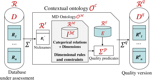
Figure 5. A contextual ontology

The contextual ontology $\mathcal{O}^{c}$ can be used to support the specification and extraction of quality data, as shown in Figure 5. A database instance $D$ for a relational schema $\mathcal{R}=\{R_{1},...,R_{n}\}$ is mapped into $\mathcal{O}^{c}$ for quality data specification and extraction. The ontology contains a copy, $\mathcal{R}^{\prime}=\{R^{\prime}_{1},...,R^{\prime}_{n}\}$, of schema $\mathcal{R}$ with predicates that are nicknames for those in $\mathcal{R}$. The nickname predicates are directly populated with the data in the corresponding relations (tables) in $D$.

In addition to the multidimensional (MD) ontology, $\mathcal{O}^{M}$, the contextual ontology contains, in ontology $\mathcal{O}^{q}$, definitions of application-dependent quality predicates $\mathcal{P}$, those in $\Sigma^{\mathcal{P}}$. Together with application-dependent, not directly dimensional rules, e.g. capturing guidelines as in Example 1.1, they capture data quality concerns. Figure 5 also shows $E$ as a possible extra contextual database, with schema $\mathcal{R}^{E}$, whose data could be used at the contextual level in combination with the data strictly associated to the multidimensional ontology (cf. Section 5 for more details).

Data originally obtained from $D$ is processed through the contextual ontology, producing, possibly virtual, extensions for copies, $R^{q}$, of the original predicates $R$ in $\mathcal{R}$. Predicates $R^{q}\in\mathcal{R}^{q}$ are the “quality versions” of predicates $R\in\mathcal{R}$. The following example shows the gist.

Example 1.2.

(ex. 1.1 cont.)  ${\it Temperatures}^{\prime}$, the nickname for predicate ${\it Temperatures}$ in the original instance, is defined by the rule:

(3) $${\it Temperatures}(t,p,v,n)\rightarrow{\it Temperatures}^{\prime}(t,p,v,n).$$

Furthermore, $\mathcal{O}^{q}$ contains rule (2) as a definition of quality predicate ${\it TakenWithTherm}$. Now, ${\it Temperatures}^{q}$, the quality-version of predicate ${\it Temperatures}$, is defined by means of:

(4) $${\it Temperatures}^{\prime}(t,p,v,n),{\it TakenWithTherm}(t,n,{\sf b1})\rightarrow{\it Temperatures}^{q}(t,p,v,n).$$

The extension of ${\it Temperatures}^{q}$ can be computed, and is shown in  Table 2. It contains “quality data” from the original relation ${\it Temperatures}$. The second and the third tuples in ${\it Temperatures}^{q}$ are obtained through the fact that Sara was in the intensive care unit on Aug/21, as reported by the last in-gray shaded tuple in WorkSchedules in Figure 4, which was created by upward data propagation with the dimensional ontology.

It is not mandatory to materialize relation ${\it Temperatures}^{q}$. Actually, the doctor’s query:

(5) $$\!\!\!\mathcal{Q}(v)\!:\exists n\;\exists t\;({\it Temperatures}(t,{\sf tom\;waits},v,n)\ \wedge\ {\sf 11\!:\!45\mbox{-}aug\mbox{/}21\mbox{/}2016}\leq t\leq{\sf 12\!:\!15\mbox{-}aug\mbox{/}21\mbox{/}2016})\vspace{-4mm}$$

oo

can be answered by, (a) replacing Temperatures by ${\it Temperatures}^{q}$, (b) unfolding the definition of ${\it Temperatures}^{q}$ in (4), obtaining a query in terms of ${\it TakenWithTherm}$ and ${\it Temperatures}^{\prime}$; and (c) using (2) and (3) to compute the answers through $\mathcal{O}^{M}$ and $D$. The quality answer is the second tuple in Table 2. (This procedure is described in general in Section 5.2). $\hfill\Box$

Due to the simple ontological rules and the use of them in the example above, we obtain a single quality instance. In other cases, we may obtain several of them, and quality query answering amounts to doing certain query answering (QA) on Datalog^± ontologies, in particular on the the MD ontologies. Query answering on Datalog^± ontologies has been investigated in the literature for different classes of Datalog^± programs. For some of them, query answering is tractable and there are efficient algorithms. For others, the problem is know to be tractable, but still practical algorithms are needed. For some classes, the problem is known to be intractable. For this reason, it becomes important to characterize the kind of Datalog^± ontologies used for the OMD model.

The promising application of the OMD model that we investigate in this work is related to data quality concerns as pertaining to the use and production of data (Batini & Scannapieco, 2006). By this we mean that the available data are not bad or good a priori or prima facie, but their quality depends on how they were created or how they will be used, and this information is obtained from a contextual ontology. This form of data quality has been mentioned in the literature. For example, in (Wang & Strong, 1996) contextual data quality dimensions are described as those quality dimensions that are relevant to the context of data usage. In (Herzog et al., 2009) and (Juran & Godfrey, 1999), quality is characterized as “fitness for use”.

Our motivating example already shows the gist of our approach to this form of data quality: Nothing looks wrong with the data in Table 1 (the data source), but in order to assess the quality of the source’s data or to extract quality data from it, we need to provide additional data and knowledge that do not exist at the source; and they are both provided by the context. From this point of view, we are implicitly addressing a problem of incomplete data, one of the common data quality dimensions (Batini & Scannapieco, 2006). However, this is not the form of explicit incompleteness that we face with null or missing values in a table (Libkin, 2014). (Cf. Section 6.3 for an additional discussion on the data quality dimensions addressed by the OMD model.)

As we pointed out before (cf. Footnote 2), our contextual approach can be used, depending on the elements we introduce in a contextual ontology, to address other data quality concerns, such as inconsistency, redundancy, and the more typical and direct form of incompleteness, say obtaining from the context data values for null or missing values in tables.

In this work we concentrate mostly on the OMD model by itself, but also on its combination and use with quality-oriented ontologies for quality QA. We do not go into data quality assessment, which is also an interesting subject. Next, we summarize the main contributions of this work.

(A)  We propose and formalize the Ontological Multidimensional Data Model (OMD model), which is based on a relational extension via Datalog^± of the HM model for multidimensional data.  The OMD allows for: (a) Categorical relations linked to dimension categories (at any level), which go beyond the bottom-level, numerical fact tables found in data warehouses. (b) Incomplete data (and complete data as usual). (c) A logical integration and simultaneous representation of dimensional data and metadata, the latter by means of semantic dimensional constrains and dimensional rules. (d) Dimensional navigation and data generation, both upwards and downwards (the examples above show only the upward case).

(B)  We establish that, under natural assumptions that MD ontologies belong to the class of weakly-sticky (WS) Datalog^± programs (Calì et al., 2012c), for which conjunctive QA is tractable (in data).  The class of W ​​S programs is an extension of sticky Datalog^±(Calì et al., 2012c)  and weakly-acyclic programs (Fagin et al., 2005). Actually, W ​​S  Datalog^± is defined through restrictions on join variables occurring in infinite-rank positions, as introduced in (Fagin et al., 2005).

In this work, we do not provide algorithms for (tractable) QA on weakly-sticky Datalog^± programs. However, in (Milani & Bertossi, 2016b) a practical algorithm was proposed, together with a methodology for magic-set- based query optimization.

(C)  We analyze the interaction between dimensional constraints and the dimensional rules, and their effect on QA. Most importantly, the combination of constraints that are equality-generating dependencies (egds) and the rules, which are tuple-generating dependencies (tgds) (Calì et al., 2003), may lead to undecidability of QA.  Separability (Calì et al., 2012c) is a semantic condition on egds and tgds that guarantees the interaction between them does not harm the tractability of QA.  Separability is an application-dependent issue. However, we show that, under reasonable syntactic conditions on egds in MD ontologies, separability holds.

(D)  We propose a general ontology-based approach to contextual quality data specification and extraction. The methodology takes advantage of a MD ontology and a process of dimensional navigation and data generation that is triggered by queries about quality data.  We show that under natural conditions the elements of the quality-oriented ontology $\mathcal{O}^{q}$, in form of additional Datalog^±rules and constraints, do not affect the good computational properties of the core MD ontology $\mathcal{O}^{M}$.

The closest work related to our OMD model can be found in the dimensional relational algebra proposed in (Martinenghi & Torlone, 2014), which is subsumed by the OMD model (Milani, 2017, chap. 4). The contextual and dimensional data representation framework in (Bolchini et al., 2013) is also close to our OMD model in that it uses dimensions for modeling context. However, in their work dimensions are different from the dimensions in the HM data model. Actually, they use the notion of context dimension trees (CDTs) for modeling multidimensional contexts. Section 6.5 includes more details on related work.

This paper is structured as follows. Section 2 contains a review of databases, Datalog^±, and the HM data model. Section 3 formalizes the OMD data model. Section 4 analyzes the computational properties of the OMD model. Section 5 extends the OMD model with additional contextual elements for specifying and extracting quality data, and show how to use the extension for this task. Section 6 discusses additional related work, draws some final conclusions, and includes a discussion of possible extensions of the OMD model.  This paper considerably extends results previously reported in (Milani & Bertossi, 2015b).

2. Background

In this section, we briefly review relational databases and the multidimensional data model.

2.1. Relational Databases

We always start with a relational schema $\mathcal{R}$ with two disjoint domains: $\mathcal{C}$, with possibly infinitely many constants, and $\mathcal{N}$, of infinitely many labeled nulls. $\mathcal{R}$ also contains predicates of fixed finite arities. If $P$ is an $n$-ary predicate (i.e. with $n$ arguments) and $1\leq i\leq n$, $P[i]$ denotes its $i$-th position. $\mathcal{R}$ gives rise to a language $\mathfrak{L}(\mathcal{R})$ of first-order (FO) predicate logic with equality ($=$). Variables are usually denoted with $x,y,z,...$, and sequences thereof by $\bar{x},...$. Constants are usually denoted with $a,b,c,...$; and nulls are denoted with $\zeta,\zeta_{1},...$. An atom is of the form $P(t_{1},\ldots,t_{n})$, with $P$ an $n$-ary predicate and $t_{1},\ldots,t_{n}$ terms, i.e. constants, nulls, or variables. The atom is ground (aka. a tuple) if it contains no variables. An instance $I$ for schema $\mathcal{R}$ is a possibly infinite set of ground atoms; this set $I$ is also called an extension for the schema. In particular, the extension of a predicate $P$ in an instance $I$, denoted by $P(I)$, is the set of atoms in $I$ whose predicate is $P$. A database instance is a finite instance that contains no nulls. The active domain of an instance $I$, denoted ${\it Adom}(I)$, is the set of constants or nulls that appear in atoms of $I$. Instances can be used as interpretation structures for language $\mathfrak{L}(\mathcal{R})$.

An instance $I$ may be closed or incomplete (a.k.a. open or partial). In the former case, one makes the meta-level assumption, the so-called closed-world-assumption (CWA) (Reiter, 1984; Abiteboul et al., 1995), that the only positive ground atoms that are true w.r.t. $I$ are those explicitly given as members of $I$. In the latter case, those explicit atoms may form only a proper subset of those positive atoms that could be true w.r.t. $I$.

A homomorphism is a structure-preserving mapping, $h\!\!:\mathcal{C}\cup\mathcal{N}\!\rightarrow\!\mathcal{C}\cup\mathcal{N}$, between two instances $I$ and $I^{\prime}$ for schema $\mathcal{R}$ such that: (a) $t\in\mathcal{C}$ implies $h(t)=t$, and (b) for every ground atom $P(\bar{t})$: if $P(\bar{t})\in I$, then $P(h(\bar{t}))\in I^{\prime}$.

A conjunctive query (CQ) is an FO formula, $\mathcal{Q}(\bar{x})$, of the form:

(6) $$\exists\bar{y}\;(P_{1}(\bar{x}_{1})\wedge\dots\wedge P_{n}(\bar{x}_{n})),$$

with $P_{i}\in\mathcal{R}$, and (distinct) free variables $\bar{x}:=\bigcup\bar{x}_{i}\smallsetminus\bar{y}$. If $\mathcal{Q}$ has $m$ (free) variables, for an instance $I$, $\bar{t}\in(\mathcal{C}\cup\mathcal{N})^{m}$  is an answer to $\mathcal{Q}$ if $I\models\mathcal{Q}[\bar{t}]$, meaning that $Q[\bar{t}]$ becomes true in $I$ when the variables in $\bar{x}$ are componentwise replaced by the values in $\bar{t}$. $\mathcal{Q}(I)$ denotes the set of answers to $\mathcal{Q}$ in $I$. $\mathcal{Q}$ is a boolean conjunctive query (BCQ) when $\bar{x}$ is empty, and if it is true in $I$, in which case $\mathcal{Q}(I):=\{{\it true}\}$. Otherwise, $\mathcal{Q}(I)=\emptyset$, and we say it is false.

A tuple-generating dependency (tgd), also called a rule, is an implicitly universally quantified sentence of $\mathfrak{L}(\mathcal{R})$ of the form:

(7) $$\sigma\!:\ \ P_{1}(\bar{x}_{1}),\ldots,P_{n}(\bar{x}_{n})\ \rightarrow\ \exists\bar{y}\ P(\bar{x},\bar{y}),$$

with $P_{i}\in\mathcal{R}$, and $\bar{x}\subseteq\bigcup_{i}\bar{x}_{i}$, and the dots in the antecedent standing for conjunctions. The variables in $\bar{y}$ (that could be empty) are the existential variables. We assume $\bar{y}\cap\cup\bar{x}_{i}=\emptyset$. With ${\it head}(\sigma)$ and ${\it body}(\sigma)$ we denote the atom in the consequent and the set of atoms in the antecedent of $\sigma$, respectively.

A constraint is an equality-generating dependency (egd  ​​) or a negative constraint (nc), which are also sentences of $\mathfrak{L}(\mathcal{R})$, respectively, of the forms:

(8) $$P_{1}(\bar{x}_{1}),\ldots,P_{n}(\bar{x}_{n})\ \rightarrow\ x=x^{\prime},$$

(9) $$P_{1}(\bar{x}_{1}),\ldots,P_{n}(\bar{x}_{n})\ \rightarrow\ \bot,$$

with $P_{i}\in\mathcal{R}$, and $x,x^{\prime}\in\bigcup_{i}\bar{x}_{i}$, and $\bot$ is a symbol that denotes the Boolean constant (propositional variable) that is always false. Satisfaction of constraints by an instance is as in FO logic. In Section 3 we will use ncs with negated body atoms (i.e. negative literals), in a limited manner. Their semantics is also as in FO logic, i.e. the body cannot be made true in a consistent instance, for any data values for the variables in it.

Tgds, egds, and ncs are particular kinds of relational integrity constraints (ICs) (Abiteboul et al., 1995). In particular, egds include key constraints and functional dependencies (FDs). ICs also include inclusion dependencies (IDs): For an $n$-ary predicate $P$ and an $m$-ary predicate $S$, the ID $P[j]\subseteq S[k]$, with $j\leq n,\ k\leq m$, means that -in the extensions of $P$ and $S$ in an instance- the values appearing in the $j$th position (attribute) of $P$ must also appear in the $k$th position of $S$.

Relational databases work under the CWA, i.e. ground atoms not belonging to a database instance are assumed to be false. As a consequence, an IC is true or false when checked for satisfaction on a (closed) database instance, never undetermined. However, as we will see below, if instances are allowed to be incomplete, i.e. with undetermined or missing ground atoms, ICs may not be false, but only undetermined in relation to their truth status. Actually, they can be used, by enforcing them, to generate new tuples for the (open) instance.

Datalog is a declarative query language for relational databases that is based on the logic programming paradigm, and allows to define recursive views (Abiteboul et al., 1995; Ceri et al., 1990). A Datalog program $\Pi$ for schema $\mathcal{R}$ is a finite set of non-existential rules, i.e. as in (7) but without $\exists$-variables. Some of the predicates in $\Pi$ are extensional, i.e. they do not appear in rule heads, and their complete extensions are given by a database instance $D$ (for a subschema of $\mathcal{R}$), that is called the program’s extensional database. The program’s intentional predicates are those that are defined by the program by appearing in tgds’ heads. The program’s extensional database $D$ may give to them only partial extensions (additional tuples for them may be computed by the application of the program’s tgds). However, without loss of generality, it is common with Datalog to make the assumption that intensional predicates do not have an explicit extension, i.e. explicit ground atoms in $D$.

The minimal-model semantics of a Datalog program w.r.t. an extensional database instance $D$ is given by a fix-point semantics (Abiteboul et al., 1995): the extensions of the intentional predicates are obtained by, starting from $D$, iteratively enforcing the rules and creating tuples for the intentional predicates, i.e. whenever a ground (or instantiated) rule body becomes true in the extension obtained so far, but not the head, the corresponding ground head atom is added to the extension under computation. If the set of initial ground atoms is finite, the process reaches a fix-point after a finite number of steps. The database instance obtained in this way turns out to be the unique minimal model of the Datalog program: it extends the extensional database $D$, makes all the rules true, and no proper subset has the two previous properties. Notice that the constants in a minimal model of a Datalog program are those already appearing in the active domain of $D$ or in the program rules; no new data values of any kind are introduced.

One can pose a CQ to a Datalog program by evaluating it on the minimal model of the program, seen as a database instance. However, it is common to add the query to the program, and the minimal model of the combined program gives us the set of answers to the query. In order to do this, a CQ as in (6) is expressed as a Datalog rule of the form:

(10) $$P_{1}(\bar{x}_{1}),...,P_{n}(\bar{x}_{n})\rightarrow{\it ans}_{\mathcal{Q}}(\bar{x}),$$

where ${\it ans}_{\mathcal{Q}}(\cdot)$ is an auxiliary, answer-collecting predicate. The answers to query $\mathcal{Q}$ form the extension of predicate ${\it ans}_{\mathcal{Q}}(\cdot)$ in the minimal model of the original program extended with the query rule. When $\mathcal{Q}$ is a BCQ, ${\it ans}_{\mathcal{Q}}$ is a propositional atom; and $\mathcal{Q}$ is true in the undelying instance exactly when the atom ${\it ans}_{\mathcal{Q}}$ belongs to the minimal model of the program.

Example 2.1.

A Datalog program $\Pi$ containing the rules  $P(x,y)~{}\rightarrow~{}R(x,y)$,  and  $P(x,y),R(y,z)$  $~{}\rightarrow~{}R(x,z)$   recursively defines, on top of an extension for predicate $P$, the intentional predicate $R$ as the transitive closure of $P$. With $D=\{P(a,b),P(b,d)\}$ as the extensional database, the extension of $R$ can be computed by iteratively adding tuples enforcing the program rules, which results in the instance $I=\{P(a,b),P(b,d),R(a,b),R(b,d),R(a,d)\}$, which is the minimal model of the program.

The CQ $\mathcal{Q}(x)\!:\ R(x,b)\wedge R(x,d)$ can be expressed by the rule  $R(x,b),R(x,d)\ \rightarrow\ {\it ans}_{\mathcal{Q}}(x)$. The set of answers is the computed extension for ${\it ans}_{\mathcal{Q}}(x)$ on instance $D$, namely $\{a\}$. Equivalently, the query rule can be added to the program, and the minimal model of the resulting program will contain the extension for the auxiliary predicate ${\it ans}_{\mathcal{Q}}$: $I^{\prime}=\{P(a,b),P(b,d),R(a,b),R(b,d),R(a,d),{\it ans}_{\mathcal{Q}}(a)\}$. $\hfill\Box$

2.2. Datalog^±

Datalog^± is an extension of Datalog. The “$+$” stands for the extension, and the “$-$”, for some syntactic restrictions on the program that guarantee some good computational properties. We will refer to some of those restrictions in Section 4. Accordingly, until then we will consider Datalog⁺ programs.

A Datalog⁺ program may contain, in addition to (non-existential) Datalog rules, also existential rules rules of the form (7), and constraints of the forms (8) and (9). A Datalog⁺ program has an extensional database $D$. In a Datalog⁺ program $\Pi$, unlike plain Datalog, predicates are not necessarily partitioned into extensional and intentional ones: any predicate may appear in the head of a rule. As a consequence, some predicates may have partial extensions in the extensional database $D$, and their extensions will be completed via rule enforcements.

The semantics of a Datalog⁺ program $\Pi$ with an extensional database instance $D$ is model-theoretic, and given by the class ${\it Mod}(\Pi,{D})$ of all, possibly infinite, instances ${I}$ for the program’s schema (in particular, with domain contained in $\mathcal{C}\cup\mathcal{N}$) that extend $D$ and make $\Pi$ true. Notice that, and in contrast to Datalog, the combination of the “open-world assumption” and the use of $\exists$-variables in rule heads makes us consider possibly infinite models for a Datalog⁺program, actually with domains that go beyond the active domain of the extensional database.

If a Datalog^± program $\Pi$ has an extensional database instance $D$, a set $\Pi^{R}$ of tgds, and a set $\Pi^{C}$ of constraints of the forms (8) or (9), then $\Pi$ is consistent if ${\it Mod}(\Pi,{D})$ is non-empty, i.e. the program has at least one model.

Given a Datalog⁺program $\Pi$ with database instance $D$ and an $n$-ary CQ $\mathcal{Q}(\bar{x})$, $\bar{t}\in(\mathcal{C}\cup\mathcal{N})^{n}$ is an answer w.r.t. $\Pi$ iff ${I}\models\mathcal{Q}[\bar{t}]$ for every ${I}\in{\it Mod}(\Pi,{D})$, which is equivalent to $\Pi\cup D\models\mathcal{Q}[\bar{t}]$. Accordingly, this is certain answer semantics. In particular, a BCQ $\mathcal{Q}$ is true w.r.t. $\Pi$ if it is true in every ${I}\in{\it Mod}(\Pi,{D})$. In the rest of this paper, unless otherwise stated, CQs are BCQs, and CQA is the problem of deciding if a BCQ is true w.r.t. a given program.

Without any syntactic restrictions on the program, and even for programs without constraints, conjunctive query answering (CQA) may be undecidable (Beeri & Vardi, 1981). CQA appeals to all possible models of the program. However, the chase procedure (Maier et al., 1979) can be used to generate a single, possibly infinite, instance that represents the class ${\it Mod}(\Pi,{D})$ for this purpose. We show it by means of an example.

Example 2.2.

Consider a program $\Pi$ with the set of rules  $\sigma\!:R(x,y)\ \rightarrow\ \exists z\ R(y,z)$,  and  $\sigma^{\prime}\!:R(x,y),R(y,z)\ \rightarrow\ S(x,y,z)$, and an extensional database instance ${D}=\{R(a,b)\}$, providing an incomplete extension for the program’s schema. With the instance $I_{0}:={D}$, the pair $(\sigma,\theta_{1})$, with (value) assignment (for variables) $\theta_{1}\!:\ x\mapsto a,y\mapsto b$, is applicable: $\theta_{1}({\it body}(\sigma))=\{R(a,b)\}\subseteq I_{0}$. The chase enforces $\sigma$ by inserting a new tuple $R(b,\zeta_{1})$ into $I_{0}$ ($\zeta_{1}$ is a fresh null, i.e. not in $I_{0}$), resulting in instance $I_{1}$.

Now, $(\sigma^{\prime},\theta_{2})$, with $\theta_{2}\!:\ x\mapsto a,y\mapsto b,z\mapsto\zeta_{1}$, is applicable, because $\theta_{2}({\it body}(\sigma^{\prime}))$ $=$ $\{R(a,b),R(b,$  $\zeta_{1})\}\subseteq I_{1}$. The chase adds $S(a,b,\zeta_{1})$ into $I_{1}$, resulting in $I_{2}$. The chase continues, without stopping, creating an infinite instance, usually called the chase (instance): ${\it chase}(\Pi,{D})=\{R(a,b),R(b,\zeta_{1}),S(a,b,\zeta_{1}),$  $R(\zeta_{1},\zeta_{2}),R(\zeta_{2},\zeta_{3}),S(b,\zeta_{1},\zeta_{2}),\ldots\}$. $\hfill\Box$

For some programs an instance obtained through the chase may be finite. Different orders of chase steps may result in different sequences and instances. However, it is possible to define a canonical chase procedure that determines a canonical sequence of chase steps, and consequently, a canonical chase instance (Calì et al., 2013).

Given a program $\Pi$ and extensional database ${D}$, its chase (instance) is a universal model (Fagin et al., 2005): For every ${I}\in{\it Mod}(\Pi,{D})$, there is a homomorphism from the chase into ${I}$. For this reason, the (certain) answers to a CQ $\mathcal{Q}$ under $\Pi$ and ${D}$ can be computed by evaluating $\mathcal{Q}$ over the chase instance (and discarding the answers containing nulls) (Fagin et al., 2005). Universal models of Datalog programs are finite and coincide with the minimal models. However, the universal model of a Datalog⁺ program may be infinite, this is when the chase procedure does not stop, as shown in Example 2.2. This is a consequence of the OWA underlying Datalog⁺ programs and the presence of existential variables.

If a program $\Pi$ consists of a set of tgds $\Pi^{R}$ and a set of ncs $\Pi^{C}$, then CQA amounts to deciding if $D\cup\Pi^{R}\cup\Pi^{C}\models\mathcal{Q}$. However, this is equivalent to deciding if: (a) $D\cup\Pi^{R}\models\mathcal{Q}$,  or  (b) for some $\eta\in\Pi^{C}$, $D\cup\Pi^{R}\models\mathcal{Q}_{\eta}$, where $\mathcal{Q}_{\eta}$ is the BCQ obtained as the existential closure of the body of $\eta$ (Calì et al., 2012c, theo. 6.1). In the latter case, $D\cup\Pi$ is inconsistent, and $\mathcal{Q}$ becomes trivially true. This shows that CQA evaluation under ncs can be reduced to the same problem without ncs, and the data complexity of CQA does not change. Furthermore, ncs may have an effect on CQA only if they are mutually inconsistent with the rest of the program, in which case every BCQ becomes trivially true.

If $\Pi$ has egds, they are expected to be satisfied by a modified (canonical) chase (Calì et al., 2013) that also enforces the egds. This enforcement may become impossible at some point, in which case we say the chase fails (cf. Example 2.3).  Notice that consistency of a Datalog⁺ program is defined independently from the chase procedure, but can be characterized in terms of the chase. Furthermore, if the canonical chase procedure terminates (finitely or by failure) the result can be used to decide if the program is consistent. The next example shows that egds may have an effect on CQA even with consistent programs.

Example 2.3.

Consider a program $\Pi$ with ${D}=\{R(a,b)\}$ with two rules and an egd:

(11) $$R(x,y)~{} \rightarrow~{}\exists z\;\exists w\;S(y,z,w).$$

(12) $$S(x,y,y)~{} \rightarrow~{}P(x,y).$$

(13) $$S(x,y,z)~{} \rightarrow~{}y=z.$$

The chase of $\Pi$ first applies (11) and results in $I_{1}=\{R(a,b),S(b,\zeta_{1},\zeta_{2})\}$. There are no more tgd/assignment applicable pairs. But, if we enforce the egd (13), equating $\zeta_{1}$ and $\zeta_{2}$, we obtain $I_{2}=\{R(a,b),S(b,\zeta_{1},\zeta_{1})\}$. Now, (12) and $\theta^{\prime}:x\mapsto b,y\mapsto\zeta_{1}$ are applicable, so we add $P(b,\zeta_{1})$ to $I_{2}$, generating $I_{3}=\{R(a,b),S(b,\zeta_{1},\zeta_{1}),P(b,\zeta_{1})\}$. The chase terminates (no applicable tgds or egds), obtaining ${\it chase}(\Pi,{D})=I_{3}$.

Notice that the program consisting only of (11) and (12) produces $I_{1}$ as the chase, which makes the BCQ $\exists x\exists y\;P(x,y)$ evaluate to false. With the program also including the egd (13) the answer is now true, which shows that consistent egds may affect CQ answers. This is in line with the use of a modified chase procedure that applies them along with the tgds.

Now consider program $\Pi^{\prime}$ that is $\Pi$ with the extra rule  $R(x,y)~{}\rightarrow~{}\exists z\;S(z,x,y)$, which enforced on $I_{3}$ results in $I_{4}=\{R(a,b),S(b,\zeta_{1},\zeta_{1}),P(b,\zeta_{1}),S(\zeta_{3},a,b)\}$. Now (13) is applied, which creates a chase failure as it tries to equate constants $a$ and $b$. This is case where the set of tgds and the egd are mutually inconsistent. $\hfill\Box$

2.3. The Hurtado-Mendelzon Multidimensional Data Model

According to the Hurtado-Mendelzon multidimensional data model (in short, the HMmodel) (Hurtado & Mendelzon, 2002), a dimension schema, $\mathscr{H}=\langle\mathscr{K},\nearrow\rangle$, consists of a finite set $\mathscr{K}$ of categories, and an irreflexive, binary relation $\nearrow$, called the child-parent relation, between categories (the first category is a child and the second category is a parent). The transitive and reflexive closure of $\nearrow$ is denoted by $\nearrow^{*}$, and is a partial order (a lattice) with a top category, All, which is reachable from every other category: $K\!\nearrow^{*}\!{\it All}$, for every category $K\in\mathscr{K}$. There is a unique base category, $K^{b}$, that has no children. There are no “shortcuts”, i.e. if $K\nearrow K^{\prime}$, there is no category $K^{\prime\prime}$, different from $K$ and $K^{\prime}$, with $K\nearrow^{*}K^{\prime\prime}$, $K^{\prime\prime}\nearrow^{*}K^{\prime}$.

A dimension instance for schema $\mathscr{H}$ is a structure $\mathscr{L}=\langle\;\!\mathcal{U},<,m\;\!\rangle$, where $\mathcal{U}$ is a non-empty, finite set of data values called members, $<$ is an irreflexive binary relation between members, also called a child-parent relation (the first member is a child and the second member is a parent), and $m\!:\mathcal{U}\rightarrow\mathscr{K}$ is the total membership function. Relation $<$ parallels (is consistent with) relation $\nearrow$: $e<e^{\prime}$ implies $m(e)\nearrow m(e^{\prime})$. The statement $m(e)=K$ is also expressed as $e\in K$. $<^{*}$ is the transitive and reflexive closure of $<$, and is a partial order over the members. There is a unique member all, the only member of All, which is reachable via $<^{*}$ from any other member: $e<^{*}{\it all}$, for every member $e$. A child member in $<$ has only one parent member in the same category: for members $e$, $e_{1}$, and $e_{2}$, if $e<e_{1}$, $e<e_{2}$ and $e_{1},e_{2}$ are in the same category (i.e. $m(e_{1})=m(e_{2})$), then $e_{1}=e_{2}$. $<^{*}$ is used to define the roll-up relations for any pair of distinct categories $K\nearrow^{*}K^{\prime}$:  $L_{K}^{K^{\prime}}(\mathscr{L})=\{(e,e^{\prime})~{}|~{}e\in K,\ e^{\prime}\in K^{\prime}\mbox{ and }e<^{*}e^{\prime}\}$.

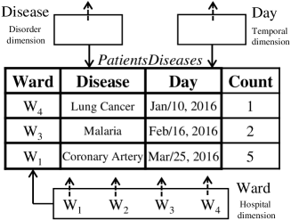
Figure 6. An HM model

Example 2.4.

The HM model in Figure 6 includes three dimension instances: Temporal and Disorder (at the top) and Hospital (at the bottom). They are not shown in full detail, but only their base categories Day, Disease, and Ward, resp. We will use four different dimensions in our running example, the three just mentioned and also Instrument (cf. Example 3.2). For the Hospital dimension, shown in detail in Figure 3, $\mathscr{K}=\{{\it Ward},{\it Unit},{\it Institution},{\it All}_{\it Hospital}\}$, with base category Ward and top category ${\it All}_{\it Hospital}$. The child-parent relation $\nearrow$ contains $({\it Institution}$  $,{\it All}_{\it Hospital})$, $({\it Unit},{\it Institution})$, and $({\it Ward},{\it Unit})$. The category of each member is specified by $m$, e.g. $m({\sf H}_{1})={\it Institution}$. The child-parent relation $<$ between members contains $({\sf W}_{1},{\sf standard})$, $({\sf W}_{2},{\sf standard})$, $({\sf W}_{3},{\sf intensive})$, $({\sf W}_{4},{\sf terminal})$, $({\sf standard},{\sf H}_{1})$, $({\sf intensive},{\sf H}_{1})$, $({\sf terminal},{\sf H}_{2})$, $({\sf H}_{1},$  ${\sf all}_{\it Hospital})$, and $({\sf H}_{2},$  ${\sf all}_{\it Hospital})$. Finally, $L_{\it Ward}^{\it Institution}$ is one of the roll-up relations and contains $({\sf W}_{1},{\sf H}_{1})$, $({\sf W}_{2},{\sf H}_{1})$, $({\sf W}_{3},{\sf H}_{1})$, and $({\sf W}_{4},{\sf H}_{2})$.$\hfill\Box$

In the rest of this section we show how to represent an HM model in relational terms. This representation will be used in the rest of this paper, in particular to extend the HM model. We introduce a relational dimension schema $\mathcal{H}=\mathcal{K}\cup\mathcal{L}$, where $\mathcal{K}$ is a set of unary category predicates, and $\mathcal{L}$ (for “lattice”) is a set of binary child-parent predicates, with the first attribute as the child and the second as the parent. The data domain of the schema is $\mathcal{U}$ (the set of category members). Accordingly, a dimension instance is a database instance $D^{\mathcal{H}}$ for $\mathcal{H}$ that gives extensions to predicates in $\mathcal{H}$. The extensions of the category predicates form a partition of $\mathcal{U}$.

In particular, for each category $K\in\mathscr{K}$ there is a category predicate $K(\cdot)\in\mathcal{K}$, and the extension of the predicate contains the members of the category. Also, for every pair of categories $K$, $K^{\prime}$ with $K\nearrow K^{\prime}$, there is a corresponding child-parent predicate, say $K\!K^{\prime}(\cdot,\cdot)$, in $\mathcal{L}$, whose extension contains the child-parent, $<$-relationships between members of $K$ and $K^{\prime}$. In other words, each child-parent predicate in $\mathcal{L}$ stands for a roll-up relation between two categories in child-parent relationship.

Example 2.5.

(ex 2.4 cont.) In the relational representation of the Hospital dimension (cf. Figure 3), schema $\mathcal{K}$ contains unary predicates ${\it Ward}(\cdot)$, ${\it Unit}(\cdot)$, ${\it Institution}(\cdot)$ and ${\it All}_{\it Hospital}(\cdot)$. The instance $D^{\mathcal{H}}$ gives them the extensions: ${\it Ward}=\{{\sf W}_{1},{\sf W}_{2},{\sf W}_{3},{\sf W}_{4}\}$, ${\it Unit}$ $=$ $\{{\sf standard},{\sf intensive},{\sf terminal}\}$, ${\it Institution}$ $=$ $\{{\sf H}_{1},{\sf H}_{2}\}$ and ${\it All}_{\it Hospital}$ $=$ $\{{\sf all}_{\it Hospital}\}$. $\mathcal{L}$ contains binary predicates: ${\it WardUnit}(\cdot,\cdot)$, ${\it UnitInstitution}(\cdot,\cdot)$, and ${\it Institution}{\it All}_{\it Hospital}(\cdot,\cdot)$, with the following extensions:   ${\it WardUnit}=\{({\sf W}_{1},$  ${\sf standard}),$ $({\sf W}_{2},{\sf standard}),$ $({\sf W}_{3},{\sf intensive}),$ $({\sf W}_{4},{\sf terminal})\}$, ${\it UnitInstitution}=\{({\sf standard},{\sf H}_{1}),$
$({\sf intensive},{\sf H}_{1}),$ $({\sf terminal},{\sf H}_{2})\}$, and ${\it InstitutionAll}_{\it Hospital}$ $=$ $\{({\sf H}_{1},{\sf all}_{\it Hospital}),$ $({\sf H}_{2},{\sf all}_{\it Hospital})\}$. $\hfill\Box$

In order to recover the hierarchy of a dimension in its relational representation, we have to impose some ICs. First, inclusion dependencies (IDs) associate the child-parent predicates to the category predicates. For example, the following IDs: ${\it WardUnit}[1]\subseteq{\it Ward}[1]$, and ${\it WardUnit}[2]\subseteq{\it Unit}[1]$. We need key constraints for the child-parent predicates, with the first attribute (child) as the key. For example, ${\it WardUnit}[1]$ is the key attribute for ${\it WardUnit}(\cdot,\cdot)$, which can be represented as the egd:  ${\it WardUnit}(x,y),{\it WardUnit}(x,z)\rightarrow y=z$.

Assume $\mathcal{H}$ is the relational schema with multiple dimensions. A fact-table schema over $\mathcal{H}$ is a predicate $T(C_{1},...,C_{n},M)$, where $C_{1},...,C_{n}$ are attributes with domains $\mathcal{U}_{i}$ for subdimensions $\mathcal{H}_{i}$, and $M$ is the measure attribute with a numerical domain. Attribute $C_{i}$ is associated with base-category predicate $K^{b}_{i}(\cdot)\in\mathcal{K}_{i}$ through the ID:  $T[i]\subseteq K^{b}_{i}[1]$. Additionally, $\{C_{1},...,C_{n}\}$ is a key for $T$, i.e. each point in the base multidimensional space is mapped to at most one measurement. A fact-table provides an extension (or instance) for $T$. For example, in the center of Figure 6, the fact table ${\it PatientsDiseases}$ is linked to the base categories of the three participating dimensions through its attributes Ward, Disease, and Day, upon which its measure attribute Count functionally depends.

This multidimensional representation enables aggregation of numerical data at different levels of granularity, i.e. at different levels of the hierarchies of categories. The roll-up relations can be used for aggregation.

3. The Ontological Multidimensional Data Model

In this section, we present the OMD model as an ontological, Datalog⁺-based extension of the HM model. In this section we will be referring to the working example from Section 1, extending it along the way when necessary to illustrate elements of the OMD model.

An OMD model has a database schema $\mathcal{R}^{\mathcal{M}}=\mathcal{H}\cup\mathcal{R}^{c}$, where $\mathcal{H}$ is a relational schema with multiple dimensions, with sets $\mathcal{K}$ of unary category predicates, and sets $\mathcal{L}$ of binary, child-parent predicates (cf. Section 2.3); and $\mathcal{R}^{c}$ is a set of categorical predicates, whose categorical relations can be seen as extensions of the fact-tables in the HM model.

Attributes of categorical predicates are either categorical, whose values are members of dimension categories, or non-categorical, taking values from arbitrary domains. Categorical predicate are represented in the form $R(C_{1},\ldots,C_{m};N_{1},\ldots,N_{n})$, with categorical attributes (the $C_{i}$) all before the semi-colon (“;”), and non-categorical attributes (the $N_{i}$) all after it.

The extensional data, i.e the instance for the schema $\mathcal{R}^{\mathcal{M}}$, is $I^{\mathcal{M}}=D^{\mathcal{H}}\cup I^{c}$, where $D^{\mathcal{H}}$ is a complete database instance for subschema $\mathcal{H}$ containing the dimensional predicates (i.e. category and child-parent predicates); and sub-instance $I^{c}$ contains possibly partial, incomplete extensions for the categorical predicates, i.e. those in $\mathcal{R}^{c}$.

Every schema $\mathcal{R}^{\mathcal{M}}=\mathcal{H}\cup\mathcal{R}^{c}$ for an OMD model comes with some basic, application-independent semantic constraints. We list them next, represented as ICs.

1.   Dimensional child-parent predicates must take their values from categories. Accordingly, if child-parent predicate $P\in\mathcal{L}$ is associated to category predicates $K,K^{\prime}\in\mathcal{K}$, in this order, we introduce IDs $P[1]\subseteq K[1]$ and $P[2]\subseteq K^{\prime}[1]$), as ncs:

(14) $$P(x,x^{\prime}),\lnot K(x)\rightarrow\bot,\ \ \ \ \mbox{ and }\ \ \ \ P(x,x^{\prime}),\lnot K^{\prime}(x^{\prime})\rightarrow\bot.$$

We do not represent them as the tgds $P(x,x^{\prime})\rightarrow K(x)$, etc., because we reserve the use of tgds for predicates (in their right-hand sides) that may be incomplete. This is not the case for $K$ or $K^{\prime}$, which have complete extensions in every instance. For this same reason, as mentioned right after introducing ncs in (8), we use here ncs with negative literals: they are harmless in the sense that they are checked against complete extensions for predicates that do not appear in rule heads. Then, this form of negation is the simplest case of stratified negation (Abiteboul et al., 1995). Checking any of these constraints amounts to posing a non-conjunctive query to the instance at hand (we retake this issue in Section 4.3).

2.  Key constraints on dimensional child-parent predicates $P\in\mathcal{K}$, as egds:

(15) $$P(x,x_{1}),P(x,x_{2})~{}\rightarrow~{}x_{1}=x_{2}.$$

3.  The connections between categorical attributes and the category predicates are specified by means of IDs represented as ncs. More precisely, for the $i$th categorical position of predicate $R$ taking values in category $K$, the ID $R[i]\subseteq K[1]$ is represented by:

(16) $$R(\bar{x};\bar{y}),\lnot K(x)~{}\rightarrow~{}\bot,$$

where $x$ is the $i$th variable in the list $\bar{x}$.

Example 3.1.

(ex. 1.1 cont.) The categorical attributes Unit and Day of categorical predicate ${\it WorkSchedules}(\!{\it Unit},\!{\it Day};\!{\it Nurse}\!,{\it Speciality})$ in $\mathcal{R}^{c}$ are connected to the Hospital and Temporal dimensions, resp., which is captured by the IDs ${\it WorkSchedules}[1]\subseteq{\it Unit}[1]$, and ${\it WorkSchedules}[2]\subseteq{\it Day}[1]$. The former is written in Datalog⁺ as in (16):

(17) $${\it WorkSchedules(u,d;n,t)},\lnot{\it Unit}(u)~{}\rightarrow ~{}\bot.$$

For the Hospital dimension, one of the two IDs for the child-parent predicate ${\it WardUnit}$ is ${\it WardUnit}[2]\subseteq{\it Unit}[1]$, which is expressed by an nc of the form (14):

$${\it WardUnit(w,u)},\lnot{\it Unit}(u)~{}\rightarrow ~{}\bot.$$

The key constraint of WardUnit is captured by an egd of the form (15):

$$\hskip 93.89418pt{\it WardUnit(w,u)},{\it WardUnit(w,u^{\prime})}~{}\rightarrow ~{}\ u=u^{\prime}.\hskip 93.89418pt\hfill\Box$$

The OMD model allows us to build multidimensional ontologies, $\mathcal{O}^{\mathcal{M}}$. Each of them, in addition to an instance $I^{\mathcal{M}}$ for a schema $\mathcal{R}^{\mathcal{M}}$, includes a set $\Omega^{\mathcal{M}}$ of basic constraints as in 1.-3. above, a set $\Sigma^{\mathcal{M}}$ of dimensional rules, and a set $\kappa^{\mathcal{M}}$ of dimensional constraints. All these rules and constraints are expressed in the Datalog⁺ language associated to schema $\mathcal{R}^{\mathcal{M}}$. Below we introduce the general forms for dimensional rules in $\Sigma^{\mathcal{M}}$ (those in 4.) and the dimensional constraints in $\kappa^{\mathcal{M}}$ (in 5.), which are all application-dependent.

4.  Dimensional rules as Datalog⁺ tgds:

(18) $$R_{1}(\bar{x}_{1};\bar{y}_{1}),...,R_{n}(\bar{x}_{n};\bar{y}_{n}),P_{1}(x_{1},x^{\prime}_{1}),...,P_{m}(x_{m},x^{\prime}_{m})\ \rightarrow\ \exists\bar{y}^{\prime}\ {R^{\prime}}({\bar{x}^{\prime}};\bar{y}).$$

Here, $R_{i}(\bar{x}_{i};\bar{y}_{i})$ and ${R^{\prime}}({\bar{x}^{\prime}};\bar{y})$ are categorical predicates, the $P_{i}$ are child-parent predicates, $\bar{y}^{\prime}\subseteq\bar{y}$,  ${\bar{x}^{\prime}}\subseteq\bar{x}_{1}\cup...\cup\bar{x}_{n}\cup\{x_{1},...,x_{m},x^{\prime}_{1},...,x^{\prime}_{m}\}$,  $\bar{y}\!\smallsetminus\!\bar{y}^{\prime}\subseteq\bar{y}_{1}\cup...\cup\bar{y}_{n}$; repeated variables in bodies (join variables) appear only in categorical positions in the categorical relations and attributes in child-parent predicates.

Notice that existential variables appear only in non-categorical attributes.  The main reason for this condition is that in some applications we may have an existing, fixed and closed-world multidimensional database providing the multidimensional structure and data. In particular, we may not want to create new category elements via value invention, but only values for non-categorical attributes, which do not belong to categories. We will discuss this condition in more detail and its possible relaxation in Section 6.4.

5.  Dimensional constraints, as egds or ncs, of the forms:

(19) $$R_{1}(\bar{x}_{1};\bar{y}_{1}),...,R_{n}(\bar{x}_{n};\bar{y}_{n}),P_{1}(x_{1},x^{\prime}_{1}),...,P_{m}(x_{m},x^{\prime}_{m})~{}\rightarrow~{} z=z^{\prime}.$$

(20) $$R_{1}(\bar{x}_{1};\bar{y}_{1}),...,R_{n}(\bar{x}_{n};\bar{y}_{n}),P_{1}(x_{1},x^{\prime}_{1}),...,P_{m}(x_{m},x^{\prime}_{m})~{}\rightarrow~{} \bot.$$

Here, $R_{i}\in\mathcal{R}^{c}$, $P_{j}\in\mathcal{L}$, and $z,z^{\prime}\in\bigcup\bar{x}_{i}\cup\bigcup\bar{y}_{j}$.

Some of the lists in the bodies of (18)-(19) may be empty, i.e. $n=0$ or $m=0$. This allows us to represent, in addition to properly “dimensional” constraints, also classical constraints on categorical relations, e.g. keys or FDs.

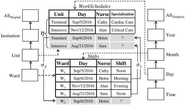
Figure 7. An OMD model with categorical relations, dimensional rules, and constraints

A general tgd of the form (18) can be used for upward- or downward-navigation (or, more precisely, upward or downward data generation) depending on the joins in the body. The direction is determined by both the difference of category levels in a dimension of the categorical variables that appear in the body joins, and the value propagation to the rule head. To be more precise, consider the simplest case where (18) is of the form

$$R(\bar{x};\bar{y}_{1}),P(x_{1},x^{\prime}_{1})\ \rightarrow\ \exists\bar{y}^{\prime}\ {R^{\prime}}({\bar{x}^{\prime}};\bar{y}),$$

with a join between $R(\bar{x};\bar{y}_{1})$ and $P(x_{1},x^{\prime}_{1})$ (via a categorical variable in $\bar{x}$). When $x_{1}\in\bar{x}$ and $x^{\prime}_{1}\in\bar{x}^{\prime}$, one-step upward-navigation is enabled, from (the level of) $x_{1}$ to (the level of) $x^{\prime}_{1}$. An example is $\sigma_{1}$ in (1). Now, when $x^{\prime}_{1}\in\bar{x}$ and $x_{1}\in\bar{x}^{\prime}$, one-step downward-navigation is enabled. An example is $\sigma_{2}$ in (22).  More generally, multi-step navigation, between a category and an ancestor or descendant category, can be captured through a chain of joins with adjacent child-parent dimensional predicates in the body of a tgd (an example is (23) below). However, a general dimensional rule of the form (18) may contain joins in mixed directions, even on the same dimension.

Example 3.2.

(ex. 3.1 cont.)   The left-hand-side of Figure 7 shows a dimensional constraint $\eta$ categorical relation WorkSchedules, which is linked to the Temporal dimension via the Day category. It tells us (possibly because the Intensive care unit was closed during January) that:  “No personnel was working in the Intensive care unit in January”. It is a constraint of the form (20):

(21) $$\eta\!:\ {\it WorkSchedules}({\sf intensive},d;n,s),{\it DayMonth}(d,{\sf jan})~{}\rightarrow~{}\bot.$$

The dimensional rule $\sigma_{1}$ in Figure 7 and given in (1) (as a tgd of the general form (18)) can be used to generate new tuples for relation WorkSchedules. Then, constraint $\eta$ is expected to be satisfied both by the initial extensional tuples for WorkSchedules and its tuples generated through $\sigma_{1}$, i.e. by its non-shaded tuples and shaded tuples in Figure 7, resp. In this example, $\eta$ is satisfied.

Notice that WorkSchedules refers to the ${\it Day}$ attribute of the Temporal dimensions, whereas $\eta$ involves the Month attribute. Then, checking $\eta$ requires upward navigation through the Temporal dimension. Also the Hospital dimension is involved in the satisfaction of $\eta$:  The tgd $\sigma_{1}$ in may generate new tuples for WorkSchedules, by upward navigation from Ward to Unit.

Furthermore, we have an additional tgd:

(22) $$\sigma_{2} : \!\!{\it WorkSchedules}(u,d;n,t),{\it WardUnit}(w,u)~{}\rightarrow~{}\exists s\;{\it Shifts}(w,d;n,s)$$

that can be used with WorkSchedules to generate data for categorical relation Shifts. The shaded tuple in it is one of those. This tgd reflects the institutional guideline stating that “If a nurse works in a unit on a specific day, he/she has shifts in every ward of that unit on the same day”.  Accordingly, $\sigma_{2}$ relies on downward navigation for tuple generation, from the Unit category level down to the Ward category level.

Here, $\sigma_{1}$ and $\sigma_{2}$ in (1) and (22) are examples of tgds enabling upward and downward, one-step dimension navigation, resp. The following dimensional rule enables multi-step navigation, propagating doctors at the unit level all the way up to the hospital level:

(23) $${\it WardDoc}({\it ward};{\it na},{\it sp}),{\it WardUnit}({\it ward,unit}),{\it UnitInst}({\it unit,ins})\rightarrow{\it HospDoc}({\it ins};{\it na},{\it sp}).$$

Assuming the ontology also has a categorical relation, ${\it Therm(Ward,Thertype};{\it Nurse})$, with Ward and Thertype categorical attributes, the latter for an ${\sf Instrument}$ dimension, the following should be an egd of the form (19) saying that “All thermometers in a unit are of the same type”:

(24) $${\it Therm(w,t;n)},{\it Therm(w^{\prime},t^{\prime};n^{\prime})},\!{\it WardUnit(w,u)},\!{\it WardUnit(w^{\prime},u)}\rightarrow t=t^{\prime}.$$

Notice that our ontological language allows us to impose a condition at the Unit level without having it as an attribute in the categorical relation.

Notice that existential variables in dimensional rules, such as $t$ and $s$ as in (1) and (22), resp., make up for the missing, non-categorical attributes Speciality and Shift in WorkSchedules and Shifts, resp.$\hfill\Box$

Example 3.3.

(ex. 3.2 cont.)  Rule $\sigma_{2}$ supports downward tuple-generation. When enforcing it on a tuple ${\it WorkSchedules}(u,d;n,t)$, via category member $u$ (for Unit), a tuple for Shifts is generated for each child $w$ of $u$ in the Ward category for which the body of $\sigma_{2}$ is true. For example, chasing $\sigma_{2}$ with the third tuple in WorkSchedules generates two new tuples in Shifts:  ${\it Shifts}({\sf W}_{2},{\sf sep/6/2016},{\sf helen},\zeta)$ and ${\it Shifts}({\sf W}_{1},{\sf sep/6/2016},{\sf helen},\zeta^{\prime})$, with fresh nulls, $\zeta$ and $\zeta^{\prime}$. The latter tuple is not shown in Figure 7 since it is dominated by the third tuple, ${\it Shifts}({\sf W}_{1},{\sf sep/6/2016},{\sf helen},{\sf morning})$, in Shifts (i.e. the existing tuple is more general or informative than the one that would be introduced with a null value, and also it already serves as a witness for the existential statement). With the old and new tuples we can obtain the answers to the query about the wards of Helen on Sep/6/2016:  $\mathcal{Q}^{\prime}(w)\!:\ \exists s\;{\it Shifts}(w,{\sf sep/6/2016},{\sf helen},s)$. They are $W_{1}$ and $W_{2}$.

In contrast, the join between Shifts and WardUnit in $\sigma_{1}$ enables upward-dimensional navigation; and the generation of only one tuple for WorkSchedules from each tuple in Shifts, because each Ward member has at most one Unit parent. $\hfill\Box$

4. Computational Properties of the OMD Model

As mentioned before, without any restrictions Datalog⁺ programs conjunctive query answering (CQA) may be undecidable, even without constraints (Calì et al., 2003). Accordingly, it is important to identify classes of programs for which CQA is decidable, and hopefully in polynomial time in the size of the underlying database, i.e. in data complexity. Some classes of this kind have been identified. In the rest of this section we introduce some of them that are particularly relevant for our research. We show that under natural assumptions or OMD ontologies belong to those classes. In general, those program classes do not consider constraints. At the end of the section we consider the presence of them in terms of their effect on QA.

4.1. Weakly-Acyclic, Sticky and Weakly-Sticky Programs

Weakly-acyclic Datalog^± programs (without constraints) form a syntactic class of Datalog⁺ programs that is defined appealing to the notion of dependency graph (Fagin et al., 2005). The dependency graph (DG) of a Datalog⁺ program $\Pi$ is a directed graph whose vertices are the positions of the program’s schema. Edges are defined as follows. For every $\sigma\in\Pi$ and universally quantified variable ($\forall$-variable) $x$ in ${\it head}(\sigma)$ and position $p$ in ${\it body}(\sigma)$ where $x$ appears:  (a) Create an edge from $p$ to position $p^{\prime}$ in ${\it head}(\sigma)$ where $x$ appears (representing the propagation of a value from a position in the body of a rule to a position in its head).  (b) Create a special edge from $p$ to position $p^{\prime\prime}$ in ${\it head}(\sigma)$ where an $\exists$-variable $z$ appears (representing a value invention in the position of an existential variable in the rule head).

The rank of a position $p$, ${\it rank}(p)$, is the maximum number of special edges on (finite or infinite) paths ending at $p$. $\pi_{F}(\Pi)$ denotes the set of finite-rank positions in $\Pi$. A program is Weakly-Acyclic (WA) if all of the positions have finite-rank.

Example 4.1.

Program $\Pi$ below has the DG in Figure  8, with dashed special edges.

Figure 8. Dependency graph

$$U(x) ~{}\rightarrow~{}\exists y\;R(x,y),$$

$$R(x,y) ~{}\rightarrow~{}P(x,y).$$

oo

$U[1]$, $R[1]$ and $P[1]$ have rank $0$.  $R[2]$ and $P[2]$ have rank $1$. Then, $\pi_{F}(\Pi)=\{U[1],R[1],P[1],R[2],P[2]\}$, and $\Pi$ is W ​​A.$\hfill\Box$

The chase for these programs stops in polynomial time in the size of the extensional data, making CQA ptime-complete in data complexity (Fagin et al., 2005), but 2exptime-complete in combined complexity, i.e. in the combined size of the program, query and data (Kolaitis et al., 2006).

Sticky Datalog⁺ programs (without constraints) are characterized through a marking procedure on body variables program rules. For a program $\Pi$, the procedure has two steps:

1. Preliminary step: For every $\sigma\in\Pi$ and variable $x$ in ${\it body}(\sigma)$, if there is an atom in ${\it head}(\sigma)$ where $x$ does not appear, mark every occurrence $x$ in ${\it body}(\sigma)$.

2. Propagation step: For every $\sigma\in\Pi$, if a marked variable in ${\it body}(\sigma)$ appears in position $p$, then for every $\sigma^{\prime}\in\Pi$, mark every occurrence of a variable in ${\it body}(\sigma^{\prime})$ that also appears in ${\it head}(\sigma^{\prime})$ in position $p$.

Example 4.2.

Consider program $\Pi$ on the left-hand side below., with its second rule already showing marked variables (with a hat) after the preliminary step. The set of rules on the right-hand side show the result of whole marking procedure.

$$\begin{array}[]{rl c rl}R(x,y),P(x,z)~{}\rightarrow&~{}S(x,y,z).&&R(\hat{x},y),P(\hat{x},\hat{z})~{}\rightarrow&~{}S(x,y,z).\\ S(\hat{x},y,\hat{z})~{}\rightarrow&~{}U(y).&&S(\hat{x},y,\hat{z})~{}\rightarrow&~{}U(y).\\ U(x)~{}\rightarrow&~{}\exists y\;R(y,x).&&U(x)~{}\rightarrow&~{}\exists y\;R(y,x).\end{array}$$

For example, $x$ is marked in $S[1]$ in the body of the second rule (after the preliminary step). For the propagation step, we find $S[1]$ in the head of the first rule, containing $x$ (it could have been a different variable). Then the occurrences of $x$ in the body of the first rule have to be marked too, in positions $R[1]$ and $P[1]$. $\hfill\Box$

A Datalog⁺ program $\Pi$ is sticky when, after applying the marking procedure, there is no rule with a marked variable appearing more than once in its body. (Notice that a variable never appears both marked and unmarked in a same body.) Accordingly, the program in Example 4.2 is not sticky: marked variable $x$ in the first rule’s body appears in a join (in $R[1]$ and $P[1]$).

The stickiness property for a program guarantees that, given a CQ, a finite initial fragment of the possibly infinite chase can be used for answering the query; actually, a fragment of polynomial size in that of the extensional data (cf. (Calì et al., 2012c) and (Milani & Bertossi, 2016b) for a more detailed discussion). As a consequence, CQA on sticky programs is in ptime in data. (It is exptime-complete in combined complexity (Calì et al., 2012c).) Even more, CQA over sticky programs enjoys first-order rewritable (Gottlob et al., 2011), that is, a CQ posed to the program can be rewritten into an FO query that can be evaluated directly on the extensional data.

None of the well-behaved classes of weakly-acyclic and sticky programs contain the other, but they can be combined into a new syntactic class of weakly-sticky (WS) programs that extends both original classes. Again, its characterization does not depend on the extensional data, and uses the already introduced notions of finite-rank and marked variable: A program $\Pi$ (without constraints) is weakly-sticky if every repeated variable in a rule body is either non-marked or appears in some position in $\pi_{F}(\Pi)$ (in that body).

Example 4.3.

Consider program $\Pi$ already showing the marked variables:

$$R(\hat{x},\hat{y})~{}\rightarrow ~{}\exists z\;R(y,z).$$

$$R(\hat{x},\hat{y}),U(\hat{y}),R(\hat{y},\hat{z})~{}\rightarrow ~{}R(x,z).$$

Here, $\pi_{F}(\Pi)=\{U[1]\}$. The only join variable is $y$ in the second rule, which appears in $U[1]$. Since $U[1]\in\pi_{F}(\Pi)$, $\Pi$ is WS.  Now, let $\Pi^{\prime}$ be obtained from $\Pi$ by replacing the second rule by (the already marked) rule:   $R(\hat{x},\hat{y}),R(\hat{y},\hat{z})~{}\rightarrow~{}R(x,z)$.  Now, $\pi_{F}(\Pi^{\prime})=\emptyset$, and the marked join variable $y$ in the second rule appears in $R[1]$ and $R[2]$, both non-finite (i.e. infinite) positions. Then, $\Pi^{\prime}$ is not WS.$\hfill\Box$

The W ​​S conditions basically prevent marked join variables from appearing only in infinite (i.e. infinite-rank) positions. With W ​​S programs the chase may not terminate, due to an infinite generation and propagation of null values, but in finite positions only finitely many nulls may appear, which restricts the values that the possibly problematic variables, i.e. those marked in joins, may take (cf. (Milani & Bertossi, 2016b) for a discussion). For W ​​S programs CQA is tractable. Actually, CQA can be done on initial, query-dependent fragments of the chase of polynomial size in data. CQA is tractable, but ptime-complete in data, and 2exptime-complete in combined complexity (Calì et al., 2012c).

In the following and as usual with a Datalog^± program $\Pi$, we say $\Pi$ is weakly-acyclic, sticky or weakly-sticky, etc., if its set of tgds has those properties.

4.2. OMD Ontologies as Weakly-Sticky Datalog^± Programs

In this section we investigate the ontologies $\mathcal{O}^{\mathcal{M}}$ used by the OMD model as Datalog^± programs. We start by considering only their subontologies $\Sigma^{\mathcal{M}}$ formed by their tgds. The impact of the set $\kappa^{\mathcal{M}}$ of constraints in $\mathcal{O}^{\mathcal{M}}$ is analyzed in Section 4.3.

It turns out that the MD ontologies are weakly-sticky. Intuitively, the main reason is that the join variables in the dimensional tgds are in the categorical positions, where finitely many members of dimensions can appear during the chase, because no existential variable ($\exists$-variable) occurs in a categorical position; so, no new values are invented in them positions during the chase.

Proposition 4.4.

MD ontologies are weakly-sticky Datalog^± programs. $\hfill\Box$

Proof of Proposition 4.4: The tgds are of the form (18):

$$R_{1}(\bar{x}_{1};\bar{y}_{1}),...,R_{n}(\bar{x}_{n};\bar{y}_{n}),P_{1}(x_{1},x^{\prime}_{1}),...,P_{m}(x_{m},x^{\prime}_{m})\ \rightarrow\ \exists\bar{y}^{\prime}\ R^{\prime}(\bar{x}^{\prime};\bar{y}),$$

where: (a) $\bar{y}^{\prime}\subseteq\bar{y}$, (b) $\bar{x}^{\prime}\subseteq\bar{x}_{1}\cup...\cup\bar{x}_{n}\cup\{x_{1},...,x_{m},x^{\prime}_{1},...,x^{\prime}_{m}\}$, (c) $\bar{y}\!\smallsetminus\!\bar{y}^{\prime}\subseteq\bar{y}_{1}\cup...\cup\bar{y}_{n}$, and (d) repeated (i.e. join) variables in bodies are only in positions of categorical attributes.

We have to show that every join variable in such a tgd either appears at least once in a finite-rank position or it is not marked. Actually, the former always holds, because, by condition (d), join variables appear only in categorical positions; and categorical positions, as we will show next, have finite, actually $0$, rank (so, no need to investigate marked positions).

In fact, condition (a) guarantees that there is no special edge in the dependency graph of a set of dimensional rules $\Sigma^{\mathcal{M}}$ that ends at a categorical position. Also, (b) ensures that there is no path from a non-categorical position to a categorical position, i.e. categorical positions are connected only to categorical positions. Consequently, every categorical position has a finite-rank, namely $0$. $\hfill\Box$

The proof establishes that every position involved in join in the body of a tgd has finite rank. However, non-join body variables in a tgd might still have infinite rank.

Example 4.5.

(ex. 3.2 cont.) For the MD ontology with $\sigma_{1}$ and $\sigma_{2}$, ${\it WorkSchedules}[4]$ and ${\it Shifts}[4]$ have infinite rank; and all the other positions have finite rank.$\hfill\Box$

Corollary 4.6.

Conjunctive query answering on MD ontologies (without constraints) can be done in polynomial-time in data complexity. $\hfill\Box$

The tractability (in data) of CQA under W ​​S programs was established in (Calì et al., 2012c) on theoretical grounds, without providing a practical algorithm. An implementable, polynomial-time algorithm for CQA under W ​​S programs is presented in (Milani & Bertossi, 2016b). Given a CQ posed to the program, they apply a query-driven chase of the program, generating a finite initial portion of the chase instance that suffices to answer the query at hand. Actually, the algorithm can be applied to a class that not only extends WS, but is also closed under magic-set rewriting of Datalog⁺ programs (Alviano et al., 2012), which allows for query-dependent optimizations of the program (Milani & Bertossi, 2016b).

Unlike sticky programs, for complexity-theoretic reasons, W ​​S programs do not allow FO rewritability for CQA. However, a hybrid algorithm is proposed in (Milani et al., 2016c). It is based on partial grounding of the tgds using the extensional data, obtaining a sticky program, and a subsequent rewriting of the query. These algorithms can be used for CQA under our MD ontologies. However, presenting the details of these algorithms is beyond the scope of this paper.

4.3. OMD Ontologies with Constraints

In order to analyze the impact of the constraints on MD ontologies, i.e. those in 1.-3., 5. in Section 3, on CQA, we have to make and summarize some general considerations on constraints in Datalog⁺ programs. First, the whole discussion on constraints of Section 2.2 apply here. In particular, the presence of constraints may make the ontology inconsistent, in which case CQA becomes trivial. Furthermore, in comparison to a program without constraints, the addition of the latter to the same program may change query answers, because some models of the ontology may be discarded. Furthermore, CQA under ncs can be reduced to CQA without them.

First, those in (14) and (16) are ncs with negative literals in their bodies. The former capture the structure of the underlying multidimensional data model (as opposed to the ontological one). They can be checked against the extensional database $D$. If they are satisfied, they will stay as such, because the dimensional tgds in (18) do not invent category members. If the underlying multidimensional database has been properly created, those constraints will be satisfied and preserved as such. The same applies to the negative constraints in (16): the dimensional tgds may invent only non-categorical values in categorical relations. (cf. Section 6.4 for a discussion.)

As discussed in Section 3, egds may be more problematic since there may be interactions between egds and tgds during the chase procedure: the enforcement of a tgd may activate an egd, which in turn may make some tgds applicable, etc. (cf. Section 2.2). Actually, these interactions between tgds and egds, make it in general impossible to postpone egd checking or enforcement until all tgds have been applied: tgd-chase steps and egd-chase steps may have to be interleaved. When the (combined) chase does not fail, the result is a possibly infinite universal model that satisfies both the tgds and egds (Calì et al., 2013).

The interaction of tgds and egds  may lead to undecidability of CQA (Calì et al., 2003; Chandra & Vardi, 1985; Johnson & Klug, 1984; Mitchell, 1983). However, a separability property of the combination of egds and tgds guarantees a harmless interaction that makes CQA decidable and preserves CQA (Calì et al., 2012c):  For a program $\Pi$ with extensional database $D$, a set of tgds $\Pi^{R}$, and a set of egds $\Pi^{C}$, $\Pi^{R}$ and $\Pi^{C}$ are separable if either (a) the chase with $\Pi$ fails, or (b) for any BCQ $\mathcal{Q}$, $\Pi\models\mathcal{Q}$ if and only if $\Pi^{R}\cup D\models\mathcal{Q}$.

In Example 2.3, the tgds and the egd are not separable as the chase does not fail, and the egd changes CQ answers (in that case, $\Pi\not\models\mathcal{Q}$ and $\Pi^{\prime}\models\mathcal{Q}$).

Separability is a semantic property, relative to the chase, and depends on a program’s extensional data. If separability holds, combined chase failure can be detected by posing BCQs (with $\neq$, and obtained from the egds’  bodies) to the program without the egds (Calì et al., 2012d, theo. 1). However, separability is undecidable (Calì et al., 2012d). Hence the need for an alternative, syntactic, decidable, sufficient condition for separability. Such a condition has been identified for egds that are key constraints (Calì et al., 2013); it is that of non-conflicting interaction. Intuitively, the condition guarantees that the tgds can only generate tuples with new key values, so they cannot violate the key dependencies.

Back to our OMD ontologies, it is easy to check that the egds of the form (15) in 2., actually key constraints, are non-conflicting, because they satisfy the first of the conditions for non-conflicting interaction. Then, they are separable from the dimensional constraints as egds.

More interesting and crucial are the dimensional constraints under 5.. They are application-dependent ncs or egds. Accordingly, the discussion in Section 4.3 applies to them, and not much can be said in general. However, for the combination of dimensional tgds and dimensional egds in OMD ontologies, separability holds when the egds satisfy a simple condition.

Proposition 4.7.

For an MD ontology $\mathcal{O}^{\mathcal{M}}$ with a set $\Sigma^{\mathcal{M}}$ of tgds as in (18) and set $\kappa^{\mathcal{M}}$ of egds as in (19), if for every egd in $\kappa^{\mathcal{M}}$ the variables in the head occur in categorical positions in the body, then separability holds. $\hfill\Box$

Proof of Proposition 4.7: Let $D^{\mathcal{M}}$ be the ontology’s extensional data. We have to show that if ${\it chase}(\mathcal{O}^{\mathcal{M}})$ does not fail, then for every BCQ $\mathcal{Q}$, ${\it chase}(\mathcal{O}^{\mathcal{M}})\models\mathcal{Q}$ if and only if ${\it chase}(\Sigma^{\mathcal{M}},D^{\mathcal{M}})\models\mathcal{Q}$.

Let’s assume that the chase with $\mathcal{O}^{\mathcal{M}}$ does not fail. As we argued before Proposition 4.4, no null value replaces a variable in a categorical position during the chase with $\mathcal{O}^{\mathcal{M}}$. For this reason, the variables in the heads of egds are never replaced by nulls. As a result, the egds can only equate constants, leading to chase failure if they are different. Since we assumed the chase with $\mathcal{O}^{\mathcal{M}}$ does not fail, the egds are never applicable during the chase or they do not produce anything new (when the two constants are indeed the same), so they can be ignored, and the same result for the chase with or without egds.$\hfill\Box$

An example of dimensional egd as in Proposition  4.7 is (24). Also the key constraints in (15) satisfy the syntactic condition. In combination with Proposition 4.4, we obtain:

Corollary 4.8.

Under the hypothesis of Proposition 4.7, CQA from an MD ontology can be done in polynomial-time in data. $\hfill\Box$

Proof of Corollary 4.8: From the proof of Proposition 4.7, we have that the ${\it chase}(\mathcal{O}^{\mathcal{M}})$ never fails, and the egds can be eliminated. Then CQA can be correctly done with the extensional database and the tgds, which can de done in polynomial time in data. $\hfill\Box$

5. Contextual Data Quality Specification and Extraction

The use of the OMD model for quality data specification and extraction generalizes a previous approach to- and work on context-based data quality assessment and extraction (Bertossi et al., 2011a, 2016), which was briefly described in Section 1. The important new element in comparison to previous work is the presence in an ontological context $\mathcal{O}^{c}$ as in Figure 5 of the core multi-dimensional (MD) ontology $\mathcal{O}^{M}$ represented by an OMD model as introduced in Section 3.

In the rest of this section we show in detail the components and use of an MD context in quality data specification and extraction, for which we refer to Figure 5. For motivation and illustration we use a running example that extends those in Sections 1 and 3.

On the LHS of Figure 5, we find a database instance, $D$, for a relational schema $\mathcal{R}=\{R_{1},...,R_{n}\}$. The goal is to specify and extract quality data from $D$. For this we use the contextual ontology $\mathcal{O}^{c}$ shown in the middle, which contains the following elements and components:

1. Nickname predicates $R^{\prime}$ in a nickname schema $\mathcal{R}^{\prime}$ for predicates $R$ in $\mathcal{R}$. These are copies of the predicates for $D$ and are populated exactly as in $D$, by means of the simple mappings (rules) forming a set $\Sigma^{\prime}$ of tgds, of the form:

   (25) $$R(\bar{x})~{}\rightarrow~{}R^{\prime}(\bar{x}).$$

   whose enforcement producing a material or virtual instance $D^{\prime}$ within $\mathcal{O}^{c}$.

2. The core MD ontology, $\mathcal{O}^{\mathcal{M}}$, as in Section 3, with an instance $I^{\mathcal{M}}=D^{\mathcal{H}}\cup I^{c}$, a set $\Sigma^{\mathcal{M}}$ of dimensional tgds, and a set $\kappa^{\mathcal{M}}$ of dimensional constraints, among them egds and ncs.

3. There can be, for data quality use, extra contextual data forming an instance $E$, with schema $\mathcal{R}^{E}$, that is not necessarily part of (or related to) the OMD ontology $\mathcal{O}^{\mathcal{M}}$. It is shown in Figure 5 on the RHS of the middle box.

4. A set of quality predicates, $\mathcal{P}$, with their definitions as Datalog rules forming a set $\Sigma^{\mathcal{P}}$ of tgds. They may be defined in terms of predicates in $\mathcal{R}^{E}$, built-ins, and dimensional predicates in $\mathcal{R}^{\mathcal{M}}$. We will assume that quality predicates in $\mathcal{P}$ do not appear in the core dimensional ontology $\mathcal{O}^{M}$ that defines the dimensional predicates in $\mathcal{R}^{\mathcal{M}}$. As a consequence, the program defining quality predicates can be seen as a “top layer”, or top sub-program, that can be computed after the core (or base) ontological program has been computed. For a quality predicate $P\in\mathcal{P}$, its definition of the form:

   (26) $$\varphi_{P}^{E}(\bar{x}),\varphi^{\mathcal{M}}_{P}(\bar{x})~{}\rightarrow~{}P(\bar{x}).$$

   Here, $\varphi_{P}^{E}(\bar{x})$ is a conjunction of atoms with predicates in $\mathcal{R}^{E}$ or plus built-ins, and $\varphi^{\mathcal{M}}_{P}(\bar{x})$ is a conjunction of atoms with predicates in $\mathcal{R}^{\mathcal{M}}$.

   Due to their definitions, quality predicates in the context can be syntactically told apart from dimensional predicates. Quality predicate reflect application dependent, specific quality concerns.

Example 5.1.

(ex. 1.1 and 3.1 cont.) Predicate for ${\it Temperatures}\in\mathcal{R}$, the initial schema, has ${\it Temperatures}^{\prime}\in\mathcal{R}^{\prime}$ as a nickname, and defined by ${\it Temperatures}(\bar{x})\rightarrow{\it Temperatures}^{\prime}(\bar{x})$. The former has Table 1 as extension in instance $D$, which is under quality assessment, and with this rule, the data are copied into the context.

The core MD ontology $\mathcal{O}^{\mathcal{M}}$ has WorkSchedules and Shifts as categorical relations, linked to the Hospital and Temporal dimensions (cf. Figure 4). $\mathcal{O}^{\mathcal{M}}$ has a set of dimensional tgds, $\Sigma^{\mathcal{M}}$, that includes $\sigma_{1}$ and $\sigma_{2}$, and also a dimensional rule defining a categorical relation WorkTimes, as a view in terms of WorkSchedules the TimeDay child-parent dimensional relation, to create data from the day level down to the time (of the day) level:

(27) $${\it WorkSchedules}(u,d;n,s),{\it TimeDay}(t,d) \rightarrow{\it WorkTimes}(u,t;n,s).$$

$\mathcal{O}^{\mathcal{M}}$ also has a set $\kappa^{\mathcal{M}}$ of dimensional constraints, including the dimensional nc and egd, (21) and (24), resp.

Now, in order to address data quality concerns, e.g. about certified nurses or thermometers, we introduce quality predicates, e.g. ${\it TakenWithTherm}$, about times at which nurses use certain thermometers, with a definition of the form (26):

(28) $${\it WorkTimes}({\sf intensive},t;n,y) \rightarrow{\it TakenWithTherm}(t,n,{\sf b1}),$$

which captures the guideline about thermometers used in intensive care units; and becomes a member of $\Sigma^{\mathcal{P}}$​ (cf. Figure 5).

In this case, we are not using any contextual database $E$ outside the MD ontology, but we could have an extension for a predicate ${\it Supply(Ins,Th)}\in\mathcal{R}^{E}$, showing thermometer brands (${\it Th}$) supplied to hospital institutions (${\it Ins}$), in the Hospital dimension. It could be used to define (or supplement the previous definition of) TakenWithTherm(t,n,th):

(29) $${\it Supply(ins,th),\!UnitInstitution(u,ins)},\!{\it WorkTimes}(u,t;n,y)\rightarrow{\it TakenWithTherm(t,n,th)}.$$

$\hfill\Box$

Now the main idea consists in using the data brought into the context via the nickname predicates and all the contextual elements to specify quality data for the original schema $\mathcal{R}$, as a quality alternative to instance $D$.

• We introduce a “quality schema”, $\mathcal{R}^{q}$, a copy of schema $\mathcal{R}$, with a predicate $R^{q}$ for each predicate $R\in\mathcal{R}$. These are quality versions of the original predicates. They are defined, and populated if needed, through quality data extraction rules that form a set, $\Sigma^{q}$ (cf. Figure  5), of Datalog rules of the form:

  (30) $$R^{\prime}(\bar{x}),\psi^{\mathcal{P}}_{R^{\prime}}(\bar{x})~{}\rightarrow~{}R^{q}(\bar{x}).$$

  Here, $\psi^{\mathcal{P}}_{R^{\prime}}(\bar{x})$ is an ad hoc for predicate $R$ conjunction of quality predicates (in $\mathcal{P}$) and built-ins. The connection with the data in the corresponding original predicate is captured with the join with its nickname predicate $R^{\prime}$.

Definitions of the initial predicates’ quality versions impose conditions corresponding to user’s data quality profiles, and their extensions form the quality data (instance).

Example 5.2.

(ex. 5.1 cont.) The quality version of the original predicate ${\it Temperatures}$ is ${\it Tempera}$-  ${\it tures}^{q}\in\mathcal{R}^{q}$, defined by:

(31) $${\it Temperatures}^{\prime}(t,p,v,n),{\it TakenWithTherm}(t,n,{\sf b1})~{}\rightarrow~{}{\it Temperatures}^{q}(t,p,v,n),$$

imposing extra quality conditions on the former. This is a definition of the form (30) in $\Sigma^{q}$ (cf. also Example 1.2). $\hfill\Box$

5.1. Computational Properties of the Contextual Ontology

In Section 4, we studied the computational properties of MD ontologies without considering additional rules defining quality predicates and quality versions of tables in $D$. In this regard, it may happen that the combination of Datalog^± ontologies that enjoy good computational properties may be an ontology without such properties (Baget et al., 2011b, 2015). Actually, in our case, the contextual ontology may not preserve the syntactic properties of the core MD ontology.

Example 5.3.

(ex.  4.5 and 5.2 cont.) To the W ​​S MD ontology containing the dimensional rules $\sigma_{1}$, $\sigma_{2}$. we can add a non-recursive Datalog rule defining a quality predicate ${\it SameShift}({\it Ward},{\it Day};{\it Nurse}_{1},$  ${\it Nurse}_{2})$ saying that ${\it Nurse}_{1}$ and ${\it Nurse}_{2}$ have the same shifts at the same ward and on the same day:

$$\sigma_{3}\!:\ {\it Shifts}(w,d;n,s),{\it Shifts}(w,d;n^{\prime},s)\ \rightarrow\ {\it SameShift}(w,d;n,n^{\prime}).$$

Now, $\Sigma=\{\sigma_{1},\sigma_{2},\sigma_{3}\}$ is not W ​​S since variable $s$ in the body of $\sigma_{3}$ is a repeated marked body variable only appearing in infinite-rank position ${\it Shifts}[4]$. This shows that the even the definition of a quality predicates in plain Datalog may break the WS  property. $\hfill\Box$

Under our layered (or modular) approach (cf. item (d) at the beginning of this section), according to which definitions in $\Sigma^{\mathcal{P}}$ and $\Sigma^{q}$ belong to Datalog programs that call predicates defined in the MD ontology $\mathcal{O}^{M}$ as extensional predicates, we can guarantee that the good computational properties of the core MD ontology still hold for the contextual ontology $\mathcal{O}^{c}$. In fact, the top Datalog program can be computed in terms of CQs and iteration starting from extensions for the dimensional predicates. In the end, all this can be done in polynomial time in the size of the initial extensional database. The data in the non-dimensional, contextual, relational instance $E$ are also called as extensional data by $\Sigma^{\mathcal{P}}$ and $\Sigma^{q}$. Consequently, this is not a source of additional complexity. Thus, even when weak-stickiness does not hold for the combined contextual ontology, CQA is still tractable.

5.2. Query-Based Extraction of Quality Data

In this section we present a methodology to obtain quality data through the context on the basis of data that has origin in the initial instance $D$. The approach is query based, i.e. queries are posed to the contextual ontology $\mathcal{O}^{c}$, and in its language. In principle, any query can be posed to this ontology, assuming one knows its elements. However, most typically a user will know about $D$’s schema $\mathcal{R}$ only, and the (conjunctive) query, $\mathcal{Q}$, will be expressed in language $\mathfrak{L}(\mathcal{R})$, but (s)he will still expect quality answers. For this reason, $\mathcal{Q}$ is rewritten into a query $\mathcal{Q}^{q}$, the quality version of $\mathcal{Q}$, that is obtained by replacing every predicate $R\in\mathcal{R}$ in it by its quality version $R^{q}$ (notice that $\mathcal{Q}^{q}$ is also conjunctive). This idea leads as to the following notion of quality answer to a query.

Definition 5.4.

Given instance $D$ of schema $\mathcal{R}$ and a conjunctive query $\mathcal{Q}\in\mathfrak{L}(\mathcal{R})$, a sequence of constants $\bar{c}$ is a quality answer to $\mathcal{Q}$ from $D$ via $\mathcal{O}^{c}$ iff  $\mathcal{O}^{c}\models\mathcal{Q}^{q}[\bar{c}]$, where $\mathcal{Q}^{q}$ is the quality version of $\mathcal{Q}$, and $\mathcal{O}^{c}$ is the contextual ontology containing the MD ontology $\mathcal{O}^{M}$, and into which $D$ is mapped via rules (25).  ${\it Q\!Ans}(\mathcal{Q},D,\mathcal{O}^{c})$ denotes the set of quality answers to $\mathcal{Q}$ from $D$ via $\mathcal{O}^{c}$. $\hfill\Box$

A particular case of this definition occurs when the query is an open atomic query, say $\mathcal{Q}\!:\ R(\bar{x})$, with $R\in\mathcal{R}$. We could define the core quality version of $D$, denoted by ${\it Core}^{q}(D)$, as the database instance for schema $\mathcal{R}$ obtained by collecting the quality answers for these queries:

(32) $${\it Core}^{q}(D):=\{R(\bar{c})~{}|~{}\mathcal{O}^{c}\models R^{q}[\bar{c}]\mbox{ and }R\in\mathcal{R}\}.$$

We just gave a model-theoretic definition of quality answer. Actually, a clean answer to a query holds in every quality instance in the class ${\it Qual}(D,\mathcal{O}^{c})$ (cf. Figure 2). This semantic definition has a computational counterpart: quality answers can be obtained by conjunctive query answering from ontology $\mathcal{O}^{c}$​, a process that in general will inherit the good computational properties of the MD ontology $\mathcal{O}^{M}$, as discussed earlier in this section.

In the rest of this section, we describe the QualityQA algorithm (cf. Algorithm 1), given a CQ $\mathcal{Q}\in\mathfrak{L}(\mathcal{R})$ and a contextual ontology $\mathcal{O}^{c}$ that imports data from instance $D$, computes ${\it Q\!Ans}(\mathcal{Q},D,\mathcal{O}^{c})$. The assumption is that we have an algorithm for CQA from the MD ontology $\mathcal{O}^{M}$. If it is a weakly-sticky Datalog^± ontology, we can use the chase-based algorithm introduced in (Milani & Bertossi, 2016b). We also assume that a separability check takes place before calling the algorithm (cf. Sections 4.3 and 6.2).

For the unfolding-based steps 2 and 3, we are assuming the predicate definitions in $\Sigma^{\mathcal{P}}$ and $\Sigma^{q}$ are given in non-recursive Datalog. Starting from the CQ $\mathcal{Q}^{q}$, unfolding results into a union of conjunctive queries (UCQs) (a union in the case predicates are defined by more than one Datalog rule). Next, according to Step 4, each (conjunctive) disjunct of $\mathcal{Q}^{\mathcal{M}}$ can be answered by the given algorithm for CQA from $\mathcal{O}^{\mathcal{M}}$ with extensional data in $E$ and $D^{\prime}$ (the latter obtained by importing $D$ into context $\mathcal{O}^{c}$). The algorithm can be applied in particular to compute the core clean version, ${\it Core}^{q}(D)$, of $D$.

Step 1: Replace each predicate $R$ in $\mathcal{Q}$ with its corresponding quality version $R^{q}$, obtaining a CQ $\mathcal{Q}^{q}$ over schema $\mathcal{R}^{q}$.

Step 2: Unfold in $\mathcal{Q}^{q}$ the definitions of quality-version predicates $R^{q}$ given by the rules (30) in $\Sigma^{q}$. Obtain a UCQ $\mathcal{Q}^{c}$ in terms of predicates in $\mathcal{R}^{\prime}\cup\mathcal{P}$ and built-ins.

Step 3: Unfold in $\mathcal{Q}^{c}$ the definitions of quality predicates given by the rules (26) in $\Sigma^{\mathcal{P}}$. Obtain a UCQ $\mathcal{Q}^{\mathcal{M}}$ in terms of predicates in $\mathcal{R}^{\prime}\cup\mathcal{R}^{E}\cup\mathcal{R}^{\mathcal{M}}$, and built-ins.

Step 4: Answer $\mathcal{Q}^{\mathcal{M}}$ by CQA (for each of $\mathcal{Q}^{\mathcal{M}}$’s disjuncts) over the extensional database $E\cup D^{\prime}$ and the MD ontology $\mathcal{O}^{\mathcal{M}}$.

ALGORITHM 1 The QualityQA algorithm

Example 5.5.

(ex. 5.2 cont.) The initial query in (5), asking for (quality) values for Tom Waits’ temperature, is, according to Step 1 of QualityQA, first rewritten into:

$$\mathcal{Q}^{q}(v)\!:\exists n\;\exists t\;({\it Temperatures^{q}(t,{\sf tom\;waits},v,n)}\;\wedge\;{\sf 11\!:\!45\mbox{-}aug\mbox{/}21\mbox{/}2016}\leq t\leq{\sf 12\!:\!15\mbox{-}aug\mbox{/}21\mbox{/}2016}),$$

which can be answered using (31) to unfold according to Step 2 of QualityQA, obtaining:

$$\mathcal{Q}^{c}(v)\!:\;\exists n\;\exists t\;( {\it Temperatures}^{\prime}(t,{\sf tom\;waits},v,n)\wedge{\it TakenWithTherm}(t,n,{\sf b1})\ \wedge$$

$$~{}~{}~{}~{}~{}~{}~{}~{}~{}~{}~{}~{}~{}~{}~{}~{}~{}~{}~{}~{}~{}~{}~{}~{}~{}~{}~{}~{}~{}~{}~{}~{}~{}~{}~{}{\sf 11\!:\!45\mbox{-}aug\mbox{/}21\mbox{/}2016}\leq t\leq{\sf 12\!:\!15\mbox{-}aug\mbox{/}21\mbox{/}2016}).$$

Step 3 of QualityQA uses the quality predicate definition (28) for unfolding, obtaining the query:

$$\mathcal{Q}^{\mathcal{M}}(v)\!:\exists n\;\exists t\;\exists y\;( {\it Temperatures}^{\prime}(t,{\sf tom\;waits},v,n)\wedge{\it WorkTimes}({\sf intensive},t;n,y)\ \wedge$$

$$~{}~{}~{}~{}~{}~{}~{}~{}~{}~{}~{}~{}~{}~{}~{}~{}~{}~{}~{}~{}~{}~{}~{}~{}~{}~{}~{}~{}~{}~{}~{}~{}~{}~{}~{}~{}~{}{\sf 11\!:\!45\mbox{-}aug\mbox{/}21\mbox{/}2016}\leq t\leq{\sf 12\!:\!15\mbox{-}aug\mbox{/}21\mbox{/}2016}),$$

expressed in terms of ${\it Temperatures}^{\prime}$, predicates in $\mathcal{R}^{\mathcal{M}}$, and built-ins.

Finally, at Step 4 of QualityQA, $\mathcal{Q}^{\mathcal{M}}$ is answered as a CQ over $\mathcal{O}^{\mathcal{M}}$ and database $D^{\prime}$, using, for example, the QA algorithms in (Milani et al., 2016c; Milani & Bertossi, 2016b).

Predicate unfolding may produce a UCQ rather than a CQ. For example, if we unfold predicate TakenWithTherm according to both definitions (28) and (29), we obtain the following UCQ:

$$\mathcal{Q}^{\mathcal{M}}(v)\!:\ \ \ \exists n\;\exists t\;\exists y\;( {\it Temperatures}^{\prime}(t,{\sf tom\;waits},v,n)\wedge{\it WorkTimes}({\sf intensive},t;n,y)\ \wedge$$

$$~{}~{}~{}~{}~{}~{}~{}~{}~{}~{}~{}~{}~{}~{}~{}~{}~{}~{}~{}~{}~{}~{}~{}~{}~{}~{}~{}~{}~{}~{}~{}~{}~{}~{}~{}~{}~{}{\sf 11\!:\!45\mbox{-}aug\mbox{/}21\mbox{/}2016}\leq t\leq{\sf 12\!:\!15\mbox{-}aug\mbox{/}21\mbox{/}2016})\ \ \ \ \ \vee$$

$$\hskip 14.22636pt\exists i\;\exists n\;\exists t\;\exists u\;\exists y\;( {\it Temperatures}^{\prime}(t,{\sf tom\;waits},v,n)\wedge{\it Supply}(i,{\sf b1})\wedge{\it UnitInstitution}(u,i)\ \wedge$$

$${\it WorkTimes}(u,t;n,y)\wedge{\sf 11\!:\!45\mbox{-}aug\mbox{/}21\mbox{/}2016}\leq t\leq{\sf 12\!:\!15\mbox{-}aug\mbox{/}21\mbox{/}2016}).$$

$\hfill\Box$

6. Discussion and Conclusions

In this paper, we started from the idea that data quality is context-dependent. As a consequence, we needed a formal model of context for context-based data quality assessment and quality data extraction. For that, we followed and extended the approach in (Bertossi et al., 2011a, 2016), by proposing ontological contexts, and embedding multidimensional (MD) data models in them. For the latter, we took advantage of our relational reconstruction of the HM data model (Hurtado & Mendelzon, 2002; Hurtado et al., 2005).

The MD data model was extended with categorical relations, which are linked to categories at different levels of dimension hierarchies, and also with dimensional constraints rules. The latter add the capability of navigating multiple dimensions in both upward and downward directions. Although not shown here (but cf. (Milani, 2017)), it is possible to include in the ontological contexts semantic constraints usually present in the HM model, such as strictness and homogeneity, which guarantee summarizability (or aggregation) for the correct computation of cube views (Hurtado & Mendelzon, 2002).

We represented MD ontologies using the Datalog^± ontological language, and we showed that they fall in the syntactic class of W ​​S Datalog^± programs, for which CQA is tractable. We also unveiled conditions under which separability of egds and rules holds.

We used and extended the MD ontologies with rules for data quality specification and extraction, and proposed a general methodology for quality data extraction via query answering. Our underlying approach to data quality is that the given database instance does not have all the necessary elements to assess the quality of data or to extract quality data. The context is used for that purpose, and provides additional information about the origin and intended use of data. Notice that from this point of view, our contexts can also be seen as enabling tailoring and focusing of given data for a particular application. This is a idea that deserves additional investigation.

Our approach to quality data specification and extraction is declarative (Fan & Geerts, 2012; Bertossi & Bravo, 2013). It uses logic-based languages, namely relational calculus, Datalog and Datalog^±to specify quality data. These languages have a precise and clear semantics and their scope of applicability can be easily analyzed. It is also independent of any procedural mechanism for quality data extraction and data cleaning, but computational methods can be extracted from (or be based on) the specifications

The implementation of the QualityQA algorithm and experiments to evaluate its performance correspond to ongoing work. The algorithm and its optimization is based on our work on QA under W ​​S programs (Milani & Bertossi, 2016b; Milani et al., 2016c).

Some important possible extensions of- and issues about our OMD data model that deserve further investigation, have to do with: (a) Having categorical attributes in categorical relations forming a key.  (b) Adopting and using a repair semantics when the MD ontology becomes inconsistent.  (c) Analyzing and implementing data quality extraction as a data cleaning or repair problem.  (d) Allowing some predicates to be closed and the related problem of non-deterministic or uncertain value invention, mainly for downwards navigation. We briefly elaborate on each of them in Sections 6.1, 6.2, 6.3 and 6.4, respectively. They correspond all to open areas of research. Hence the speculative style of the discussion.

6.1. Categorical Keys

In our running example, the categorical relation WorkSchedules(Unit,Day;Nurse,Speciality), does not have $\{{\it Unit},{\it Day}\}$ as a key: multiple nurses might have work schedules in the same unit and on the same day. However, in many applications it may make sense to have the categorical attributes forming a key for a categorical relation. (For example, in the HM model, the non-measure attributes in a fact-table form a key.) This is not required by the basic OMD model, and such a key constraint has to be added.

If we assume that in a categorical relation $R(C_{1},...,C_{n};A_{1},...,A_{m})$,  $\{C_{1},...,C_{n}\}$ is a key for $R$, we have to include egds in the MD ontology, one for each pair $y_{i}\in\bar{y}$, $y^{\prime}_{i}\in\bar{y}^{\prime}$:

(33) $$R(\bar{x};\bar{y}),R(\bar{x};\bar{y}^{\prime})~{}\rightarrow~{}y^{\prime}_{i}=y_{i}.$$

We can use our running example to show that dimensional rules and categorical keys of the form (33) may not be separable (cf. Section 4.3).

Example 6.1.

Consider the categorical relation InstitutionBoard(Institution;Chair, President,CEO) with Institution as a key. In particular, we have the egd:

$${\it InstitutionBoard}(i;c,p,e),{\it InstitutionBoard}(i;c^{\prime},p^{\prime},e^{\prime})~{}\rightarrow~{}c^{\prime}=c.$$

We also have the dimensional rules (they differ on the underlined $\exists$-variables on the RHS):

(34) $${\it PatientUnit}(u,d;p),{\it UnitInstiution}(u,i)\rightarrow\exists c\;\exists n\;{\it InstitutionBoard}(i;c,\underline{c},n).$$

(35) $${\it PatientUnit}(u,d;p),{\it UnitInstiution}(u,i)\rightarrow\exists c\;\exists n\;{\it InstitutionBoard}(i;c,\underline{n},n).$$

Let $({\sf standard},{\sf sep/5};{\sf tom\;waits})$ be the only tuple in the extension of PatientUnit. The egds defining Institution as a key are not separable from the dimensional tgds (34) and (35) (cf. Section 4.3), because: (a) the chase does not fail since the egds only equate nulls invented by (34) and (35), and (b) the BCQ $\mathcal{Q}:\exists i\;\exists c\;{\it InstitutionBoard}(i,c,c,c)$ has a negative answer without the categorical key, but a positive answer with the categorical key. Actually, the combination of tgds and egds here is conflicting (cf. Section 4.3), because no $\exists$-variable in (34) or (35) appears in a key position, and then the tgds may generate different tuples with the same key values. $\hfill\Box$

Despite the possible non-separability introduced by categorical keys, CQA is still in ptime in data complexity, because no null value appears in categorical positions. As a consequence, there are polynomially many (in the size of data) key categorical values. There are also polynomially many tgd-chase steps, including those that are applicable after the egd-chase steps or due to non-separability. This shows that the chase procedure, with tgd- and egd-chase steps (as we explained in Sections 2.2) runs in polynomial time for an MD ontology under categorical keys, and CQA  can be done on the resulting chase instance.

Proposition 6.2.

The data complexity of CQA on MD ontologies with categorical keys is in ptime.$\hfill\Box$

6.2. Inconsistent MD Ontologies

We discussed in Section 4.3 the presence of dimensional ncs and egds may lead to an inconsistent MD ontology (cf. Section 2.2). In this case, the ontology can be repaired according to an inconsistency-tolerant semantics, so that it still gives semantically meaningful and non-trivial answers to queries under inconsistency. A common approach to DL or Datalog^± ontology repair has been based on repairing the extensional database in the case of Datalog^± (Lukasiewicz et al., 2012), and the A-Box in the case of DL (Lembo et al., 2010; Rosati, 2011; Bienvenu at al., 2014; Lembo et al., 2015; Bienvenu at al., 2016) ontologies.

According to this semantics, a repair of an inconsistent ontology $\mathcal{O}$ including an extensional instance $I$, is a consistent ontology with the same rules and constraints as $\mathcal{O}$, but with an extensional instance $I^{\prime}$ that is maximally contained in $I$. The consistent answers to a query posed to $\mathcal{O}$ are those answers shared by all the repairs of the latter. QA under this semantics is np-hard in the size of $I$, already for DL (Lembo et al., 2015) or Datalog^± ontologies (Lukasiewicz et al., 2012, 2015) with relatively low expressive power.

Repairing the inconsistent ontology by changing the extensional instance amounts, in the case of an MD ontology $\mathcal{O}^{M}$, to possibly changing the MD instance. In this regard, we might want to respect the MD structure of data, in particular, semantic constraints that apply at that level, e.g. enforcing summarizability constraints mentioned earlier in this section. Repairs and consistent answers from MD databases have been investigated in (Bertossi et al., 2009; Ariyan & Bertossi, 2011, 2013), and also in (Yaghmaie et al., 2012), which proposes the path schema for MD databases as a better relational schema for dealing with the kinds of inconsistencies that appear in them.

6.3. Quality Data Extraction as Inconsistency Handling

As pointed out in Section 1, context-based quality data extraction is reminiscent of database repairing and consistent query answering (Bertossi, 2011b, 2006). Actually, we can reproduce from our context-based approach to data cleaning a scenario where cleaning can be seen as consistent query answering.

The initial database $D$ may not be subject to integrity constraints. However, as we can see in Example 5.2, the rule (31) could be seen as a rewriting of the query $\mathcal{Q}(t,p,v,n)\!:\ {\it Temperatures}^{\prime}(t,p,v,n)$, performed to obtain the consistent answers (or consistent contents of Temperatures’ in this case) w.r.t. the contextual inclusion dependency  $\psi\!:\ {\it Temperatures}^{\prime}(t,p,v,n)\rightarrow{\it TakenWithTherm}(t,n,{\sf b1})$. The rewriting reflects a repair semantics based on deletions of tuples from ${\it Temperatures}^{\prime}$ when the constraint is not satisfied (Bertossi, 2011b). That is, predicate ${\it TakenWithTherm}(t,n,{\sf b1})$ acts as a filter on predicate ${\it Temperatures}^{\prime}$.

The quality version ${\it Core}^{q}(D)$ of the initial instance $D$, defined in (32), can be seen then as the intersection of all repairs of $D$ w.r.t. these contextual constraints (more precisely, as the intersection of the instances in ${\it Qual}(D,\mathcal{O}^{c})$). Doing quality (or consistent) query answering directly from the intersection of all repairs is sound, but possibly incomplete. However, this has been a predominant approach to OBDA with inconsistent ontologies (Lembo et al., 2015; Lukasiewicz et al., 2012, 2015): the ontology is repaired by repairing the extensional instance and considering the intersection of its repairs (cf. also Section 6.2).

In Section 1 we characterized our context-based approach to data quality mainly as one confronting incompleteness of data. However, we can also see it as addressing inconsistency w.r.t. constraints imposed at the contextual level rather than directly at the database level.

6.4. Categorical Value Invention and Closed Predicates

We assumed in Section 3 that tgds do not have existential quantifiers on variables for categorical attributes. This has two important consequences. First, the OMD programs become weakly-sticky (cf. Proposition 4.4); second, we can apply the CWA to categories and categorical attributes (actually, without existential quantifications on categorical attributes, making the CWA or the OWA does not matter for CQA). Relaxing this condition has two immediate effects on the MD ontology: (a) We cannot make the CWA on dimension categories (and categorical attributes) anymore (without violating the ncs in (16)); and (b) The set of tgds of an OMD ontology may not be weakly-sticky anymore. The following example shows both issues.

Table 3. DischargePatients

	Inst.	Day	Patient
1	$H_{1}$	Sep/9	Tom Waits
2	$H_{1}$	Sep/6	Lou Reed
3	$H_{2}$	Oct/5	Elvis Costello
4	$H_{1}$	Dec/16	Elvis Costello

Table 4. PatientUnit

	Unit	Day	Patient
1	Standard	Sep/5	Tom Waits
2	Standard	Sep/9	Tom Waits
3	Intensive	Sep/6	Lou Reed

Example 6.3.

Consider categorical relations DischargePatients (Table 4) and PatientUnit (Table 4), containing data on patients leaving an institution and on locations of patients, resp. Since, a patient was in a unit when discharged, we can use DischargePatient to generate data for PatientUnit, at the Unit level, down from the Institution level, through the tgd (with a conjunction in the head that can be eliminated),

(36) $${\it DischargePatients}(i,d;p)~{}\rightarrow~{}\exists u\;({\it UnitInstitution(u,i)}\wedge{\it PatientUnit(u,d;p)}),$$

which invents values downwards, in the categorical position (for units) ${\it PatientUnit}[1]$ and in the child-parent predicate UnitInstitution in its head. This may invent new category members, which could be in conflict with the a CWA applied to category predicates, child-parent predicates, and indirectly via the ncs, to categorical attributes.

Let’s now add the following tgds, respectively, saying that every patient eventually leaves the hospital, and defining the patients’ relationships of being on a day in the same unit.

(37) $${\it PatientUnit(u,d;p)},{\it UnitInstitution(u,i)}~{} \rightarrow~{}\exists d^{\prime}{\it DischargePatients}(i,d^{\prime};p),$$

(38) $${\it PatientUnit(u,d;p)},{\it PatientUnit(u,d;p^{\prime})}~{} \rightarrow~{}{\it SameDay}(d;p,p^{\prime}),$$

The set of rules (36)-(38) is not weakly-sticky.$\hfill\Box$

If we accept value invention in OMD ontologies, then their weak-stickiness cannot be guaranteed, and has to be analyzed for each particular ontology. However, the issue raised by the example in relation to the invention of category members still persists.

Sometimes an existential quantifier is used to refer to an unspecified element in a specified set or domain, as a disjunction over its elements. This interpretation of quantifiers is possible if we have a metalevel CWA assumption or a domain closure axioms (Reiter, 1984) over (some) predicates, none of which is part of Datalog^±.

Recent work in OBDA addresses this problem, allowing the combination of open and closed predicates in Datalog^± ontologies, but previously tractable CQA may become intractable (Ahmetaj et al., 2016a). Similar extensions and results hold for light-weight DLs (Seylan et al., 2009; Franconi et al., 2011; Lutz et al., 2013, 2015).

In our case, if we accept value invention for category members, the natural candidates to be declared as closed in the new setting are the unary category predicates and the child-parent predicates: we do not want to create new category members or new children for a given parent, nor, under upward data propagation, a new parent for a given child since parents are unique, as captured by the “upward” egds (15), which will force the invented nulls to take the given parent values. More problematic becomes downward data propagation with existential quantifiers over categorical positions. Even under a closure assumption on child-parent predicates, we may end up creating new children (we stand for existing do not have any “downward” egds).

If we accept tgds such as (36) and we consider category predicates and child-parent predicates as closed, then we start departing from the usual Datalog^± semantics, and some of the results we have for weakly-sticky programs (with OWA semantics) have to be reconsidered.

Having existential variables over categorical predicates may lead to new forms of inconsistency, involving category values. Adopting a repair semantic based on changes on the extensional data leads to repairs of a MD database, which should be treated as such and not as an ordinary relational database (cf. Section 6.2).

As an alternative to existential categorical variables as choices from given (possibly closed) sets of values, we could think of using disjunctive Datalog^±, with disjunctive tgds (Alviano et al., 2012; Bourhis et al., 2015), in particular for downward navigation. However, CQA under disjunctive sticky-Datalog^± may be undecidable in some cases (Gottlob et al., 2015; Morak, 2014). Furthermore, disjunctive rule heads may become data dependant.

6.5. Related Work

As a logical extension of a multidimensional data model, our model is similar in spirit to the data warehouse conceptual data model (Franconi & Sattler, 1999) that extends the entity-relationship data model with dimensions by means of the expressive description logic (DL) $\mathcal{ALCFI}$ (Horrocks & Sattler, 1999). They concentrate on the model and reasoning about the satisfiability of the MD schema and implied statements, but not OBDA. In (Malaki et al., 2012), preliminary work motivated by data quality on specifying MD ontologies in light-weight DLs is reported, without going much into quality aspects or query answering.

The existing declarative approaches to data quality (Bertossi & Bravo, 2013) mostly use classic ICs, such as FDs and IDs, and denial constraints (i.e. the ncs of Datalog^±). Newer classes of dependencies have been introduced to capture data quality conditions and directly support data cleaning processes (Fan, 2008). Examples are conditional dependencies (conditional FDs and IDs), and matching dependencies (Fan et al., 2009, 2011). We claim that more expressive contexts are necessary in real life databases to express stronger conditions and semantics of (quality) data.

Models of context (Bolchini et al., 2007a) have been proposed and investigated in the data management and knowledge representation literature. Concentrating mostly on the former, in the following we briefly review, in an itemized manner, some of those models. After describing them, we make comparisons with our model of context and its use.

A.  Multi Context Systems (MCS) (Giunchiglia & Serafini, 1994) and Local Models Semantics (LMS) (Ghidini & Giunchiglia, 2001; ghidini, ) are related logic-based frameworks for formalizing contexts and reasoning with them. MCS provides a proof-theoretic framework with a hierarchy of FO languages, each of them for knowledge representation and reasoning within a specific context. LMS is a model-theoretic framework based on the principles of locality, i.e. reasoning uses only part (the context) of what is potentially available; and compatibility of the kinds of reasoning performed in different contexts.

B.  In (Motschnig, 1995, 2000), a general framework is proposed based on the concept of viewing for decomposing information bases into possibly overlapping fragments, called contexts, in order to be able to better manage and customize information. Viewing refers to giving partial information on conceptual entities by observing them from different viewpoints or situations.

C.  In (Analyti et al., 2007; Theodorakis et al., 2002), a model of contexts in information bases is proposed. A context is defined as a set of objects, each of them with possibly several names. Operations, such as create, copy, merge, and browse, are defined for manipulating and using contexts. Contextual objects can be structured through traditional abstraction mechanisms, i.e. classification, generalization, and attribution. A theory of contextualized information bases is introduced. It includes a set of validity constraints for contexts, a model theory, as well as a set of sound and complete inference rules.

D.  In (Ghidini & Serafini, 1998), ideas from (Ghidini & Giunchiglia, 2001), specially LMS, are applied to information integration and federated database management, where each database may have its own local semantics. LMS for federated databases is used, as an extension of LMS. A notion of logical consequence between formulae (queries) in different databases is defined, and becomes the theoretical basis for the implementation of algorithms for query answering and their optimization.

E.  Context-aware data tailoring (Bolchini et al., 2009) proposes context dimension trees (CDTs) for modeling multidimensional aspects of context. It allows sub-dimensions with values of finer granularity. A user’s context is modeled as a “chunk configuration”, consisting of a set of dimension labels and their assigned values, and is used to specify the relevant portion of a target database for the user. This user’s view is computed by combining the sub-views linked to dimension values (Bolchini et al., 2007b, 2013).

F.  In (Martinenghi & Torlone, 2014) dimensions, as in multidimensional databases, are used for modeling contexts. A context-aware data model is proposed in which the notion of context is implicit and indirectly captured by contextual attributes, i.e. relational attributes that take as values members of dimension categories. In particular, in a contextual relation the context of a tuple is captured by its values in dimensions, while the categories of these members specify the granularity level of the context. They present a query language that extends the relational algebra, by introducing new operators for manipulating the granularity of contextual attributes.

G.  In (Pitoura et al., 2011; Stefanidis et al., 2011) contexts are used in preference database systems to support context-aware queries whose results depend on the context at the time of their submission. Data cubes are used to store the dependencies between context-dependent preferences, database relations, and OLAP techniques for processing context-aware queries. This allows for the manipulation of the captured context data at various levels of abstraction.

H.  The context relational model (CR) model (Rousoss et al., 2005) extends the relational model with contexts, which are treated as first-class citizens, at the level of database models and query languages. A relation in this model has different schemas and extensions in different contexts. A set of basic operations is introduced that extend relational algebra so as to take context into account.

In the following we compare our OMD contexts with the context models in  D.-H., which have been used in data management and are relatively close to ours.

Our model of context is relational in that data are represented as relations only. However, the relational context models described above are not completely relational: they use an extension of relations with new data entities. In H., a collection of relations represents a contextual relation. Accordingly, creating, manipulating and querying those contextual relations requires additional tools and care. In E.-G., no relational representation of dimensions is given. The formalizations of context in F.-G. use a MD data model for modeling dimensions, and those in E. propose CDTs and chunk configurations, which are not represented by relational terms.

With respect to languages for querying context, E.-H. use extensions of relational algebra, from which shortcomings are inherited, in particular, the lack of recursion queries and the inability to capture incomplete data. Both features are supported the OMD model. The work under D. studies and formalizes the problem of querying federated databases using the notion of logical consequence.  OMD extends the work in F. and its query language (cf. (Milani, 2017, chap. 4)).

Concerning the applications of these context models, the context model in G. can be used in particular for context-aware preference databases. Context-aware data tailoring E. is a methodology for managing small databases (possibly obtained from larger sources) aimed at being hosted by portable devices. The work in  D. focuses on using LMS for federated databases. It is not clear how these models can be adapted for other purposes. The work on context-aware databases in F. is fairly general and can be applied in many applications in data management. Our MD context model is not restricted to the problem of data quality specification and extraction, and can have wide applicability. However, it is an open problem to find ways to provide and include in OMD the specific applications and tools that those other models provide.

References

- Abiteboul et al. (1995) Abiteboul, S., Hull, R. and Vianu, V. Foundations of Databases. Addison-Wesley, 1995.
- Ahmetaj et al. (2016a) Ahmetaj, S., Ortiz, M. and Šimkus, M. Polynomial Datalog Rewritings for Ontology Mediated Queries with Closed Predicates. In Proc. of the Alberto Mendelzon International Workshop on Foundations of Data Management (AMW), CEUR-WS Proc. Vol. 1644, 2016.
- Alviano et al. (2012) Alviano, M., Faber, W., Leone, N. and Manna, M. Disjunctive Datalog with Existential Quantifiers: Semantics, Decidability, and Complexity Issues. Theory and Practice of Logic Programming (TPLP), 2012, 12(4-5): 701-718.
- Alviano et al. (2012) Alviano, M., Leone, N., Manna, M., Terracina, G. and Veltri, P. Magic-Sets for Datalog with Existential Quantifiers. In Proc. of the Int. Conference on Datalog in Academia and Industry 2.0, 2012, Springer LNCS 7494, pp. 31-43.
- Analyti et al. (2007) Anality, A., Theodorakis, M., Spyratos, N. and Constantopoulos, P. Contextualization as an Independent Abstraction Mechanism for Conceptual Modeling. Information Systems, 2007, 32(1): 24-60.
- Ariyan & Bertossi (2011) Ariyan, S. and Bertossi, L. Structural Repairs of Multidimensional Databases. In Proc. of the Alberto Mendelzon International W S of Foundations of Data Management (AMW), 2011. CEUR-WS, Vol-749.
- Ariyan & Bertossi (2013) Ariyan, S. and Bertossi, L. A Multidimensional Data Model with Subcategories for Flexibly Capturing Summarizability. In Proc. of the International Conference on Scientific and Statistical Database Management (SSDBM), 2013.
- Baget et al. (2011b) Baget, J. F., Leclére, M., Mugnier, M.L. and Salvat, E. On Rules with Existential Variables: Walking the Decidability Line. Artificial Intelligence, 2011, 175(9-10): 1620-1654.
- Baget et al. (2015) Baget, J. F., Bienvenu, M., Mugnier, M.L. and Rocher, S. Combining Existential Rules and Transitivity: Next Steps. In Proc. of the International Joint Conference on Artificial Intelligence (IJCAI), 2015, pp. 2720-2726.
- Bahmani et al. (2012) Bahmani, Z., Bertossi, L., Kolahi, S. and Lakshmanan, L. Declarative Entity Resolution via Matching Dependencies and Answer Set Programs. In Proc. of the International Conference on Principles of Knowledge Represenattion and Reasoning (KR), 2012, AAAI Press, pp. 380-390.
- Barcelo (2009) Barcelo, P. Logical Foundations of Relational Data Exchange. ACM SIGMOD Record, 2009, 38(1):49-58.
- Batini & Scannapieco (2006) Batini, C. and Scannapieco, M. Data Quality: Concepts, Methodologies and Techniques. Second edition, Springer, 2016.
- Beeri & Vardi (1981) Beeri, C. and Vardi, M. Y. The Implication Problem for Data Dependencies. In Proc. of the Colloquium on Automata, Languages and Programming (ICALP), 1981, Springer LNCS 115, pp. 73-85.
- Bertossi (2006) Bertossi, L. Consistent Query Answering in Databases. ACM Sigmod Record, June 2006, 35(2):68-76.
- Bertossi et al. (2009) Bertossi, L., Bravo, L. and Caniupan, M. Consistent Query Answering in Data Warehouses. In Proc. of the Alberto Mendelzon International Workshop on Foundations of Data Management (AMW), 2009. CEUR-WS, Vol-450.
- Bertossi et al. (2011a) Bertossi, L., Rizzolo, F. and Lei, J. Data Quality is Context Dependent. In Proc. of the Workshop on Enabling Real-Time Business Intelligence (BIRTE) Collocated with the International Conference on Very Large Data Bases (VLDB), Springer LNBIP 84, 2011, pp. 52-67.
- Bertossi (2011b) Bertossi, L. Database Repairing and Consistent Query Answering. Morgan & Claypool, 2011.
- Bertossi & Bravo (2013) Bertossi, L. and Bravo, L. Generic and Declarative Approaches to Data Quality Management. In Handbook of Data Quality - Research and Practice, 2013, Springer, pp. 181-211, DOI: 10.1007/978-3-642-36257-6_9.
- Bertossi et al. (2016) Bertossi, L. and Rizzolo, F. Contexts and Data Quality Assessment. Corr Arxiv Paper cs.DB/1608.04142, 2016.
- Bienvenu at al. (2014) Bienvenu M., Bourgaux, C. and Goasdouè, F. Querying Inconsistent Description Logic Knowledge Bases under Preferred Repair Semantics. In Proc. of the National Conference on Artificial Intelligence (AAAI), 2014, pp. 996-1002.
- Bienvenu at al. (2016) Bienvenu M., Bourgaux, C. and Goasdouè, F. Explaining Inconsistency-tolerant Query Answering over Description Logic Knowledge Bases. In Proc. of the National Conference on Artificial Intelligence (AAAI), 2016, pp. 900-906.
- Bolchini et al. (2007a) Bolchini, C., Curino, C. A., Quintarelli, E., Schreiber, F. A. and Tanca, L. A Data-Oriented Survey of Context Models. ACM SIGMOD Record, 2007, 36(4): 19-26.
- Bolchini et al. (2007b) Bolchini, C., Quintarelli, E., Rossato, R. and Tanca, L. Using Context for the Extraction of Relational Views. In Proc. of the International and Interdisciplinary Conference on Modeling and Using Context, 2007, pp. 108-121.
- Bolchini et al. (2009) Bolchini, C., Curino, C. A., Quintarelli, E., Schreiber, F. A. and Tanca, L. Context Information for Knowledge Reshaping. International Journal of Web Engineering and Technology, 2009, 5(1): 88-103.
- Bolchini et al. (2013) Bolchini, C., Quintarelli, E. and Tanca, L. CARVE: Context-Aware Automatic View Definition over Relational Databases. Information Systems, 2013, 38(1): 45-67.
- Bourhis et al. (2015) Bourhis, P., Manna, M., Morak, M. and Pieris, A. Guarded-Based Disjunctive Tuple-Generating Dependencies. ACM Trans. Database Syst., 2016, 41(4).
- Calì et al. (2003) Calì, A., Lembo, D. and Rosati, R. On the Decidability and Complexity of Query Answering over Inconsistent and Incomplete Databases. In Proc. of the ACM SIGMOD-SIGACT Symposium on Principles of Database Systems (PODS), 2003, pp. 260-271.
- Calì et al. (2009) Calì, A., Gottlob, G. and Lukasiewicz, T. Datalog±: A Unified Approach to Ontologies and Integrity Constraints. In Proc. of the International Conference on Database Theory (ICDT), 2009, pp. 14-30.
- Calì et al. (2012c) Calì, A., Gottlob, G. and Pieris, A. Towards More Expressive Ontology Languages: The Query Answering Problem. Artificial Intelligence, 2012, 193:87-128.
- Calì et al. (2012d) Calì, A., Console, M. and Frosini, R. On Separability of Ontological Constraints. In Proc. of the Alberto Mendelzon International Workshop on Foundations of Data Management (AMW), 2012, CEUR-WS Proc. Vol. 866, pp. 48-61.
- Calì et al. (2013) Calì, A., Gottlob, G. and Kifer, M. Taming the Infinite Chase: Query Answering under Expressive Relational Constraints. Journal of Artificial Intelligence Research (JAIR), 2013, 48(1): 115-174.
- Caniupan and Bertossi (2010) Caniupan-Marileo, M. and Bertossi, L. The Consistency Extractor System: Answer Set Programs for Consistent Query Answering in Databases. Data & Knowledge Engineering, 2010, 69(6):545-572.
- Ceri et al. (1990) Ceri, S., Gottlob, G. and Tanca, L. Logic Programming and Databases. Springer, 1990.
- Chandra & Vardi (1985) Chandra, A.K. and Vardi, M.Y. The Implication Problem for Functional and Inclusion Dependencies. SIAM Journal of Computing, 1985, 14(3): 671-677.
- Eckerson (2002) Eckerson, W. Data Quality and the Bottom Line: Achieving Business Success Through a Commitment to High Quality Data. Report of the Data Warehousing Institute, 2002.
- Enderton (2001) Enderton, H. B. A Mathematical Introduction to Logic. 2nd Edition, Academic Press, 2001.
- Fagin et al. (2005) Fagin, R., Kolaitis, P. G., Miller, R. J. and Popa, L. Data Exchange: Semantics and Query Answering. Theoretical Computer Science (TCS), 2005, 336(1): 89-124.
- Fan (2008) Fan, W. Dependencies Revisited for Improving Data Quality. In Proc. of the ACM SIGMOD-SIGACT Symposium on Principles of Database Systems (PODS), 2008, pp. 159-170.
- Fan & Geerts (2012) Fan, W. and Geerts, F. Foundations of Data Quality Management. Morgan & Claypool, 2012.
- Fan (2015) Fan, W. Data Quality: From Theory to Practice. SIGMOD Record, 2015, 44(3):7-18.
- Fan et al. (2009) Fan, W., Jia, X., Li, J. and Ma, S. Reasoning about Record Matching Rules. In Proc. VLDB Endowment (PVLDB), 2009, 2(1): 407-418.
- Fan et al. (2011) Fan, W., Gao, H., Ji, X., Li, J. and Ma, S. Dynamic Constraints for Record Matching. The International Journal on Very Large Data Bases (VLDBJ), 2009, 20(4): 495-520.
- Franconi & Sattler (1999) Franconi, E. and Sattler, I. A DataWarehouse Conceptual Data Model for Multidimensional Aggregation. In Proc. of the International Workshop on Design and Management of Data Warehouses (DMDW), 1999, Article No. 13.
- Franconi et al. (2011) Franconi, E., Garcia, Y. and Seylan, I. Query Answering with DBoxes is Hard. Electronic Notes in Theoretical Computer Science (ENTCS), 2011, 278(1): 71-84.
- Ghidini & Serafini (1998) Ghidini, C. and Serafini, L. Model Theoretic Semantics for Information Integration. In Proc. of the International Conference on Artificial Intelligence, Methodology, Systems, and Applications (AIMSA), 1998, Springer LNAI Vol. 1480, pp. 267-280.
- Ghidini & Giunchiglia (2001) Ghidini, C. and Giunchiglia, F. Local Models Semantics, or Contextual Reasoning = Locality + Compatibility. Artificial Intelligence, 2001, 127(1): 221-259.
- (47) Ghidini, C. and Serafini, L. Multi-Context Logics - A General Introduction. In Context in Computing, Brézillon, P. and Gonzalez, A. J. (eds.), Springer, 2014, pp. 381-399.
- Giunchiglia & Serafini (1994) Giunchiglia, F. and Serafini, L. Multilanguage Hierarchical Logics, or: How We Can Do without Modal Logics. Artificial Intelligence, 1994, 65(1): 29-70.
- Gottlob et al. (2011) Gottlob, G., Orsi, G. and Pieris, A. Ontological Queries: Rewriting and Optimization. In Proc. of the International Conference on Data Engineering (ICDE), 2011, pp. 2-13.
- Gottlob et al. (2015) Gottlob, G., Morak, M. and Pieris, A. Recent Advances in Datalog±. Reasoning Web 2015, Springer LNCS 9203, 2015, pp. 193-217.
- Herzog et al. (2009) Herzog, T., Scheuren, F. and Winkler, W. Data Quality and Record Linkage Techniques. Springer, 2009.
- Horrocks & Sattler (1999) Horrocks, I. and Sattler, S. A Description Logic with Transitive and Inverse Roles and Role Hierarchies. ACM Transactions on Database Systems (TODS), 1999, 9(3): 385-410.
- Hurtado & Mendelzon (2002) Hurtado, C. and Mendelzon, A. OLAP Dimension Constraints. In Proc. of the ACM SIGMOD-SIGACT Symposium on Principles of Database Systems (PODS), 2002, pp. 169-179.
- Hurtado et al. (2005) Hurtado, C., Gutierrez, C. and Mendelzon, A. Capturing Summarizability with Integrity Constraints in OLAP. ACM Transactions on Database Systems (TODS), 2005, 30(3): 854-886.
- Imielinski & Lipski (1984) Imielinski, T. and Lipski, W. Incomplete Information in Relational Databases. Journal of the ACM, 1984, 31(4): 761-791.
- Jensen et al. (2010) Jensen, Ch. S., Bach Pedersen, T. and Thomsen, Ch. Multidimensional Databases and Data Warehousing. Morgan & Claypool, 2010.
- Jiang et al. (2008) Jiang, L., Borgida, A. and Mylopoulos, J. Towards a Compositional Semantic Account of Data Quality Attributes. In Proc. International Conference on Conceptual Modeling (ER), 2008, pp. 55-68.
- Johnson & Klug (1984) Johnson, D. S. and Klug, A. Testing Containment of Conjunctive Queries under Functional and Inclusion Dependencies. In Proc. of the ACM SIGMOD-SIGACT Symposium on Principles of Database Systems (PODS), 1984, pp. 164-169.
- Juran & Godfrey (1999) Juran, J.M. and A.M. Godfrey. Juran’s Quality Handbook, Fifth Edition. McGraw-Hill, 1999.
- Kolaitis et al. (2006) Kolaitis, P. G., Tan, W. C. and Panttaja, J. The Complexity of Data Exchange. In Proc. of the ACM SIGMOD-SIGACT Symposium on Principles of Database Systems (PODS), 2006, pp. 30-39.
- Lembo et al. (2010) Lembo, D., Lenzerini M., Rosati, R., Ruzzi, M. and Savo, D. F. Inconsistency-Tolerant Semantics for Description Logics. In Proc. of the International Conference on Web Reasoning and Rule Systems (RR), 2010, pp. 103-117.
- Lembo et al. (2015) Lembo, D., Lenzerini M., Rosati, R., Ruzzi, M. and Savo, D. F. Inconsistency-tolerant Query Answering in Ontology-Based Data Access. Journal of Web Semantics, 2015, 3:3-29.
- Lenzerini (2002) Lenzerini, M. Data Integration: A Theoretical Perspective. In Proc. of the ACM SIGMOD-SIGACT Symposium on Principles of Database Systems (PODS), 2002, pp. 233-246.
- Libkin (2014) Libkin, L. Incomplete Data: What Went Wrong, and How to Fix It. Proc. of the ACM SIGMOD-SIGACT Symposium on Principles of Database Systems (PODS), pp. 1-13.
- Lukasiewicz et al. (2012) Lukasiewicz, T., Martinez, M., Pieris, A. and Simari, G. Inconsistency Handling in Datalog+/- Ontologies. In Proc. of the European Conference on Artificial Intelligence (ECAI), 2012, pp. 558-563.
- Lukasiewicz et al. (2015) Lukasiewicz, T., Martinez, M., Pieris, A. and Simari, G. From Classical to Consistent Query Answering under Existential Rules. In Proc. of the National Conference on Artificial Intelligence (AAAI), 2015, pp. 1546-1552.
- Lutz et al. (2013) Lutz, C., Seylan, I. and Wolter, F. Ontology-Based Data Access with Closed Predicates is Inherently Intractable (Sometimes). In Proc. of the International Joint Conference on Artificial Intelligence (IJCAI), 2013, pp. 1024-1030.
- Lutz et al. (2015) Lutz, C., Seylan, I. and Wolter, F. Ontology-Mediated Queries with Closed Predicates. In Proc. of the International Joint Conference on Artificial Intelligence (IJCAI), 2015, pp. 3120-3126.
- Malaki et al. (2012) Malaki, A., Bertossi, L. and Rizzolo, F. Multidimensional Contexts for Data Quality Assessment. In Proc. of the Alberto Mendelzon International Workshop on Foundations of Data Management (AMW), 2012. CEUR-WS, Vol-866.
- Maier et al. (1979) Maier, D., Mendelzon, A. and Sagiv, Y. Testing Implications of Data Dependencies. ACM Transactions on Database Systems (TODS), 1979, 4(4): 455-469.
- Martinenghi & Torlone (2014) Martinenghi, D. and Torlone, R. Taxonomy-Based Relaxation of Query Answering in Relational Databases. The International Journal on Very Large Data Bases (VLDBJ), 2014, 23(5): 747-769.
- Mitchell (1983) Mitchell, J. The Implication Problem for Functional and Inclusion Dependencies. Information and Control, 1983, 56(1): 154-173.
- Milani & Bertossi (2015b) Milani, M. and Bertossi, L. Ontology-Based Multidimensional Contexts with Applications to Quality Data Specification and Extraction. In Proc. of the International Symposium on Rules and Rule Markup Languages for the Semantic Web (RuleML), Springer LNCS 9202, 2015, pp. 277-293.
- Milani & Bertossi (2016b) Milani, M. and Bertossi, L. Extending Weakly-Sticky Datalog±: Query-Answering Tractability and Optimizations. In Proc. of the International Conference on Web Reasoning and Rule Systems (RR), Springer LNCS 9898, 2016, pp. 128-143.
- Milani et al. (2016c) Milani, M., Bertossi, L. and Calì, A. A Hybrid Approach to Query Answering under Expressive Datalog±. In Proc. of the International Conference on Web Reasoning and Rule Systems (RR), Springer LNCS 9898, 2016, pp. 144-158.
- Milani (2017) Milani, M. Multidimensional Ontologies for Contextual Quality Data Specification and Extraction. PhD in Computer Science Thesis, Carleton University, 2017. http://people.scs.carleton.ca/~bertossi/papers/mostafaFinal.pdf
- Morak (2014) Morak, M. The Impact of Disjunction on Reasoning under Existential Rules. PhD in Computer Science Thesis, University of Oxford, 2015.
- Motschnig (1995) Motschnig-Pitrik, R. An Integrating View on the Viewing Abstraction: Contexts and Perspectives in Software Development, AI, and Databases. Systems Integration, 1995, 5(1): 23-60.
- Motschnig (2000) Motschnig-Pitrik, R. A Generic Framework for the Modeling of Contexts and its Applications. Data Knowledge Engineering, 2000, 32(2): 145-180.
- Pitoura et al. (2011) Pitoura, E., Stefanidis, K. and Vassiliadis, P. Contextual Database Preferences. IEE Data Engineering Bulletin, 2011, 34(2): 19-26.
- Poggi et al. (2008) Poggi, A., Lembo, D., Calvanese, D., De Giacomo, G., Lenzerini, M. and Rosati, R. Linking Data to Ontologies. Data Semantics, 2008, 10(1): 133-173.
- Rabin (1965) Rabin, M. O. A Simple Method for Undecidability Proofs and Some Applications. In Logic, Methodology and Philosophy of Science, Proceedings of the 1964 International Congress, Bar-Hillel, Y. (ed.). Studies in Logic and the Foundations of Mathematics. North-Holland Publishing Company, Amsterdam 1965, pp. 38-68.
- Redman (1998) Redman, T. The Impact of Poor Data Quality on the Typical Enterprise. Communications of the ACM, 1998, 41(2): 79-82.
- Reiter (1984) Reiter, R. Towards a Logical Reconstruction of Relational Database Theory. In On Conceptual Modelling, Springer, 1984, pp. 191-233.
- Rosati (2011) Rosati, R. On the Complexity of Dealing with Inconsistency in Description Logic Ontologies. In Proc. of the International Joint Conference on Artificial Intelligence (IJCAI), 2011, pp. 1057-1062.
- Rousoss et al. (2005) Rousoss, Y., Stavrakas, Y. and Pavlaki, V. Towards a Context-Aware Relational Model. In Proc. International Workshop on Context Representation and Reasoning, 2005, CEUR-WS, Vol-136, pp. 5-17.
- Seylan et al. (2009) Seylan, I., Franconi, E. and De Bruijn, J. Effective Query Rewriting with Ontologies over DBoxes. In Proc. of the International Joint Conference on Artificial Intelligence (IJCAI), 2009, pp. 923-925.
- Stefanidis et al. (2011) Stefanidis, K., Pitoura, E. and Vassiliadis, P. Managin Contextual Preferences. Information Systems, 2011, 36(8): 1158-1180.
- Theodorakis et al. (2002) Theodorakis, M., Anality, A., Constantopoulos, P. and Spyratos, N. A Theory of Contexts in Information Bases. Information Systems, 2002, 27(3): 151-191.
- Wang & Strong (1996) Wang R. Y. and Strong D. M. Beyond Accuracy: What Data Quality Means to Data Consumers. Journal of Management Information Systems, 1996, 12(4): 5-33.
- Yaghmaie et al. (2012) Yaghmaie, M., Bertossi, L. and Ariyan, S. Repair-Oriented Relational Schemas for Multidimensional Databases. In Proc. of the International Conference on Extending Database Technology (EDBT), 2012.