A multivariate variable selection approach for analyzing LC-MS metabolomics data

Abstract.

Omic data are characterized by the presence of strong dependence structures that result either from data acquisition or from some underlying biological processes. In metabolomics, for instance, data resulting from Liquid Chromatography-Mass Spectrometry (LC-MS) – a technique which gives access to a large coverage of metabolites – exhibit such patterns. These data sets are typically used to find the metabolites characterizing a phenotype of interest associated with the samples. However, applying some statistical procedures that do not adjust the variable selection step to the dependence pattern may result in a loss of power and the selection of spurious variables. The goal of this paper is to propose a variable selection procedure in the multivariate linear model that accounts for the dependence structure of the multiple outputs which may lead in the LC-MS framework to the selection of more relevant metabolites. We propose a novel Lasso-based approach in the multivariate framework of the general linear model taking into account the dependence structure by using various modelings of the covariance matrix of the residuals. Our numerical experiments show that including the estimation of the covariance matrix of the residuals in the Lasso criterion dramatically improves the variable selection performance. Our approach is also successfully applied to a LC-MS data set made of African copals samples for which it is able to provide a small list of metabolites without altering the phenotype discrimination. Our methodology is implemented in the R package MultiVarSel which is available from the CRAN (Comprehensive R Archive Network).

Keywords: Variable selection, high-dimension, multivariate linear model, metabolomics.

1. Introduction

Metabolomics aims to provide a global snapshot (quantitative or qualitative) of the metabolism at a given time and by extension, a phenotypic information, see Nicholson et al. (1999). To this end, it studies the concentration in small molecules called metabolites that are the end products of the enzymatic machinery of the cell. Indeed, minor variations in gene or protein expression levels that are not observable via high throughput experiments may have an influence on the metabolites and hence on the phenotype of interest. Thus, metabolomics is a promising approach that can advantageously complement usual transcriptomic and proteomic analyses.

In metabolomics, the analysis of the biological samples is often performed using High Resolution Mass Spectrometry (HRMS), Nuclear Magnetic Resonance (NMR) or Liquid Chromatography-Mass Spectrometry (LC-MS) and produces a large number of features (hundreds or thousands) that can explain a difference between two or more populations, see Zhang et al. (2012). It is well-known that the identification of metabolites discriminating these populations remains a major bottleneck in metabolomics and therefore the selection of relevant features (variables) is a crucial step in the statistical analysis of the metabolomic data, as explained in Verdegem et al. (2016).

Different supervised machine learning approaches have been used in metabolomics during the last few years, see Saccenti et al. (2013); Ren et al. (2015); Boccard and Rudaz (2016). Among them the most widely used is the partial least squares-discriminant analysis (PLS-DA) which has recently been extended to sPLS-DA (sparse partial least squares-discriminant analysis) by Lê Cao et al. (2011) to include a variable selection step. Nevertheless, Grissa et al. (2016) highlight the need for new development in the process of features selection that would take into account the specificity of metabolomics data which is the dependence that may exist between the different metabolites. In this perspective, our paper proposes a novel feature selection methodology which consists in a variable selection approach based on the Lasso criterion in a multivariate setting taking into account the dependence that may exist between the different metabolites.

More precisely, let us consider a classical metabolomics experiment where $n$ samples have been collected and analyzed. This results in an $n\times q$ data matrix where $q$ stands for the number of metabolites. When the $n$ samples have been obtained under various conditions, we are typically interested in understanding the effect of each condition on each metabolite. In the case where $C$ experimental conditions are compared, $n_{c}$ denotes the number of replicates under condition $c$, where $c\in\{1,\dots C\}$ and $\sum_{c=1}^{C}n_{c}=n$. We further denote $Y_{c,r}^{(j)}$ the centered LC-MS signal obtained for the $j$th metabolite ($j\in\{1,\dots q\}$) under Condition $c$ for Replicate $r$ ($r\in\{1,\dots n_{c}\}$). In the following, the set of conditions will be called the “factor”, each specific condition being a “level” of this factor. The most popular model to analyze quantitative observations $Y$ as a function of a qualitative variable, that is a factor, is the analysis of variance (ANOVA) model, which we write here as follows:

$$Y_{c,r}^{(j)}=\mu_{c}^{(j)}+E_{c,r}^{(j)},$$ (1)

where the observations $\{Y_{c,r}^{(j)}\}$ are assumed to be centered, so that $\mu_{c}^{(j)}$ can be interpreted as the effect of Condition $c$ (Level $c$) on Metabolite $j$ and where the residual terms $\{E_{c,r}^{(j)}\}$ are assumed to be independent and identically distributed (i.i.d.) zero-mean Gaussian random variables. The goal of such a modeling is to highlight which effects among the $\mu_{1}^{(j)},\mu_{2}^{(j)},\dots,\mu_{C}^{(j)}$ are the most significant for the metabolite $j$ since the $\{Y_{c,r}^{(j)}\}$ are assumed to be centered.

When the whole $n\times q$ data matrix is considered instead of a single column $j$, the model can be summarized in the following matrix form:

$$\boldsymbol{Y}=\boldsymbol{X}\boldsymbol{B}+\boldsymbol{E},$$ (2)

where $\boldsymbol{Y}=(Y_{i,j})_{1\leq i\leq n,\;1\leq j\leq q}$ is the $n\times q$ observation matrix, $\boldsymbol{X}$ is the $n\times p$ design matrix, $\boldsymbol{B}$ is the $p\times q$ coefficient matrix and $\boldsymbol{E}=(E_{i,j})_{1\leq i\leq n,\;1\leq j\leq q}$ is the $n\times q$ matrix of residual errors. Observe that $p$ corresponds to the number of explicative variables, which is simply $C$ in Model (1). For notational simplicity, the indices $c,r$ in $Y_{c,r}^{(j)}$ are summarized in a unique index $i$ in $\{1,\dots n\}$.

In this paper, we pay a special attention to the potential dependence that may exist among the columns of $\boldsymbol{Y}$, namely the different metabolites. To this aim, we shall assume that for each $i$ in $\{1,\dots,n\}$,

$$(E_{i,1},\dots,E_{i,q})\sim\mathcal{N}(0,\boldsymbol{\Sigma}_{q}),$$ (3)

where $\boldsymbol{\Sigma}_{q}$ denotes the covariance matrix of the $i$th row of the residual error matrix. Note that the model defined by (2) and (3) is usually called a general linear model or a multivariate linear model which has been extensively studied in Mardia et al. (1979).

The simplest assumption regarding the dependence structure of the noise is $\boldsymbol{\Sigma}_{q}=\sigma^{2}\boldsymbol{I}_{q}$, where $\boldsymbol{I}_{q}$ denotes the $q\times q$ identity matrix. In this case the different columns of $\boldsymbol{Y}$ are assumed to be independent. In more general cases, the matrix $\boldsymbol{\Sigma}_{q}$ models the dependence between the different columns of $\boldsymbol{Y}$, namely the dependence between the metabolites. In the following, we shall moreover assume that $(E_{i,1},\ldots,E_{i,q})$ and $(E_{k,1},\ldots,E_{k,q})$ are independent, when $i\neq k$, which means that the individuals are assumed to be independent.

The problem of finding which parameters are significant among the $(\mu_{c}^{(j)})_{1\leq c\leq C,1\leq j\leq q}$ in Model (1) boils down to finding the non null coefficients in the matrix $\boldsymbol{B}$ in Model (2) and hence can be seen as a variable selection problem in the general linear model. Several approaches can be considered for solving this issue: either a posteriori methods such as classical statistical tests in ANOVA models, see Mardia et al. (1979); Faraway (2004) or methods embedding the variable selection such as Lasso-type methodologies initially proposed by Tibshirani (1996). However, a raw application of such approaches does not take into account the potential dependence between the different columns of $\boldsymbol{Y}$. This drawback will be illustrated in Section 3.

The goal of our paper is twofold: First, to remedy the limitations of these approaches by proposing a method for estimating the dependence between the columns of $\boldsymbol{Y}$ and second, to deal with the potentially high number of variables by using a Lasso-type approach taking into account this dependence. For this purpose, we shall propose a three-step inference strategy further detailed hereafter.

The paper is organized as follows. Our method is described in Section 2. To support our methodology, some numerical experiments on synthetic data are provided in Section 3. Finally, an application to a metabolomics data set produced by the analysis of African copals samples is given in Section 4.

2. Statistical inference

The strategy that we propose can be summarized as follows.

• First step: Fitting a one-way ANOVA to each column of the observation matrix $\boldsymbol{Y}$ in order to have access to an estimation $\widehat{\boldsymbol{E}}$ of the residual matrix $\boldsymbol{E}$.

• Second step: Estimating the matrix $\boldsymbol{\Sigma}_{q}$ by using the methods described in Sections 2.1.1 and 2.1.2. Then, choosing the most convenient estimator $\widehat{\boldsymbol{\Sigma}}_{q}$ thanks to a statistical test described in Section 2.1.3.

• Third step: Thanks to the estimator $\widehat{\boldsymbol{\Sigma}}_{q}$, transforming the data in order to remove the dependence between the columns of $\boldsymbol{Y}$. Such a transformation will be called “whitening” hereafter. Then, applying to these transformed observations the Lasso approach described in Section 2.2.

The first step provides a first estimate $\widetilde{\boldsymbol{B}}$ of $\boldsymbol{B}$. An estimate of the residual matrix is then defined as $\widehat{\boldsymbol{E}}=\boldsymbol{Y}-\boldsymbol{X}\widetilde{\boldsymbol{B}}$. In the following, we shall focus on the last two steps.

2.1. Estimation of the dependence structure of $\boldsymbol{E}$

We propose hereafter to model each row of $\boldsymbol{E}$ as realizations of a stationary process and hence we shall use time-series models in order to describe the dependence structure of $\boldsymbol{E}$. We refer the reader to Brockwell and Davis (1991) for further details on time series modeling.

We shall consider hereafter a large variety of models ranging from the simplest parametric to the most general nonparametric dependence modeling. In each case we focus on the estimation of $\boldsymbol{\Sigma}_{q}^{-1/2}$ since using the following transformation:

$$\boldsymbol{Y}\;\boldsymbol{\Sigma}_{q}^{-1/2}=\boldsymbol{X}\boldsymbol{B}\;\boldsymbol{\Sigma}_{q}^{-1/2}+\boldsymbol{E}\;\boldsymbol{\Sigma}_{q}^{-1/2}$$ (4)

removes the dependence between the columns of $\boldsymbol{Y}$. Such a procedure will be called “whitening” hereafter.

2.1.1. Parametric dependence

The simplest model among the parametric models is the autoregressive process of order 1 denoted AR(1). More precisely, for each $i$ in $\{1,\dots,n\}$, $E_{i,t}$ satisfies the following equation:

$$E_{i,t}-\phi_{1}E_{i,t-1}=W_{i,t},\textrm{ with }W_{i,t}\sim WN(0,\sigma^{2}),$$ (5)

where $\phi_{1}$ is a real number and $WN(0,\sigma^{2})$ denotes a zero-mean white noise process of variance $\sigma^{2}$, namely, if $Z_{t}~{}\sim~{}WN(0,\sigma^{2})$, then $\mathbb{E}(Z_{t})=0$, $\mathbb{E}(Z_{t}Z_{t^{\prime}})=0$ if $t\neq t^{\prime}$ and $\mathbb{E}(Z_{t}^{2})=\sigma^{2}$.

In this case, the inverse of the square root of the covariance matrix $\boldsymbol{\Sigma}_{q}$ of $(E_{i,1},\dots,E_{i,q})$ has a simple closed-form expression given by

$$\boldsymbol{\Sigma}_{q}^{-1/2}=\left(\begin{matrix}\sqrt{1-\phi_{1}^{2}}&-\phi_{1}&0&\cdots&0\\ 0&1&-\phi_{1}&\cdots&0\\ 0&0&\ddots&\ddots&\vdots\\ \vdots&\vdots&\ddots&\ddots&-\phi_{1}\\ 0&0&\cdots&0&1&\end{matrix}\right).$$ (6)

Hence, to obtain the expression of $\widehat{\boldsymbol{\Sigma}}_{q}^{-1/2}$, it is enough to have an estimation of the parameter $\phi_{1}$ and to replace it in (6). For this, we use the estimator $\widehat{\boldsymbol{E}}$ of the residual errors matrix obtained by fitting a standard ANOVA model to the observations, which corresponds to the first step of our method. Then $\phi_{1}$ is estimated by $\widehat{\phi}_{1}$ defined by

$$\widehat{\phi}_{1}=\frac{1}{n}\sum_{i=1}^{n}\widehat{\phi}_{1,i},$$

where $\widehat{\phi}_{1,i}$ denotes the estimator of $\phi_{1}$ obtained by the classical Yule-Walker equations from $(\widehat{E}_{i,1},\dots,\widehat{E}_{i,q})$, see Brockwell and Davis (1991) for more details.

More generally, it is also possible to have access to $\boldsymbol{\Sigma}_{q}^{-1/2}$ for more complex processes such as the ARMA($p,q$) process defined as follows: For each $i$ in $\{1,\dots,n\}$,

$$E_{i,t}-\phi_{1}E_{i,t-1}-\dots-\phi_{p}E_{i,t-p}=W_{i,t}+\theta_{1}W_{i,t-1}+\dots\theta_{q}W_{i,t-q},$$ (7)

where $W_{i,t}\sim WN(0,\sigma^{2})$, the $\phi_{i}$’s and the $\theta_{i}$’s are real numbers.

2.1.2. Nonparametric dependence case

In the situation where a parametric modeling is not relevant for $\boldsymbol{\Sigma}_{q}$, it can be estimated by

$$\widehat{\boldsymbol{\Sigma}}_{q}=\left(\begin{matrix}\widehat{\gamma}(0)&\widehat{\gamma}(1)&\cdots&\widehat{\gamma}(q-1)\\ \widehat{\gamma}(1)&\widehat{\gamma}(0)&\cdots&\widehat{\gamma}(q-2)\\ \vdots&&&\\ \widehat{\gamma}(q-1)&\widehat{\gamma}(q-2)&\cdots&\widehat{\gamma}(0)\end{matrix}\right),$$ (8)

with

$$\widehat{\gamma}(h)=\frac{1}{n}\sum_{i=1}^{n}\widehat{\gamma}_{i}(h),$$

where $\widehat{\gamma}_{i}(h)$ is the standard autocovariance estimator of $\gamma_{i}(h)=\mathbb{E}(E_{i,t}E_{i,t+h})$, for all $t$. Usually, $\widehat{\gamma}_{i}(h)$ is referred to as the empirical autocovariance of the $\widehat{E}_{i,t}$’s at lag $h$ (i.e. the empirical covariance between $(\widehat{E}_{i,1},\dots,\widehat{E}_{i,n-h})$ and $(\widehat{E}_{i,h+1},\dots,\widehat{E}_{i,n})$). For a definition of the standard autocovariance estimator we refer the reader to Chapter 7 of Brockwell and Davis (1991). The matrix $\widehat{\boldsymbol{\Sigma}}_{q}^{-1/2}$ is then obtained by inverting the Cholesky factor of $\widehat{\boldsymbol{\Sigma}}_{q}$.

2.1.3. Choice of the whitening modeling

In order to decide which dependence modeling is the most adapted to the data at hand we propose hereafter a statistical test. If the whitening modeling used is well chosen then each row of $\widetilde{\boldsymbol{E}}=\widehat{\boldsymbol{E}}\widehat{\boldsymbol{\Sigma}}_{q}^{-1/2}$ should be a white noise.

One of the most popular approach for testing whether a random process is a white noise is the Portmanteau test which is based on the Bartlett theorem, for further details we refer the reader to (Brockwell and Davis, 1991, Theorem 7.2.2). By this theorem, we get that under the null hypothesis $(H_{0})$: “For each $i$ in $\{1,\dots,n\}$, $(\widetilde{E}_{i,1},\ldots,\widetilde{E}_{i,q})$ is a white noise”,

$$q\sum_{h=1}^{H}\widehat{\rho}_{i}(h)^{2}\approx\chi^{2}(H),\textrm{ as }q\to\infty,$$ (9)

for each $i$ in $\{1,\dots,n\}$, where $\widehat{\rho}_{i}(h)$ denotes the empirical autocorrelation of $(\widetilde{E}_{i,t})_{t}$ at lag $h$ and $\chi^{2}(H)$ denotes the chi-squared distribution with $H$ degrees of freedom. Thus, by (9), we have at our disposal a $p$-value for each $i$ in $\{1,\dots,n\}$ that we denote by $\textrm{Pval}_{i}$. In order to have a single $p$-value instead of $n$, we shall consider

$$q\sum_{i=1}^{n}\sum_{h=1}^{H}\widehat{\rho}_{i}(h)^{2}\approx\chi^{2}(nH),\textrm{ as }q\to\infty,$$ (10)

where the approximation comes from the fact that the rows of $\widetilde{\boldsymbol{E}}$ are assumed to be independent. Equation (10) thus provides a $p$-value: Pval. Hence, if $\textrm{Pval}<\alpha$, the null hypothesis $(H_{0})$ is rejected at the level $\alpha$, where $\alpha$ is usually equal to 5%. In such a situation taking the dependence into account and estimating the dependence by one of the previous methods should highly improve the modeling and the variable selection step.

2.2. Estimation of $\boldsymbol{B}$

2.2.1. Lasso based approach

Let us first explain briefly the usual framework in which the Lasso approach is used. We consider a high-dimensional linear model of the following form

$$\mathcal{Y}=\mathcal{X}\mathcal{B}+\mathcal{E},$$ (11)

where $\mathcal{Y}$, $\mathcal{B}$ and $\mathcal{E}$ are vectors. Note that, in high-dimensional linear models, the matrix $\mathcal{X}$ has usually more columns than rows which means that the number of variables is larger than the number of observations but $\mathcal{B}$ is usually a sparse vector, namely it contains a lot of null components.

In such models a very popular approach initially proposed by Tibshirani (1996) consists in using the Least Absolute Shrinkage eStimatOr (LASSO) criterion for estimating $\mathcal{B}$ defined as follows for a positive $\lambda$:

$$\widehat{\mathcal{B}}(\lambda)=\textrm{Argmin}_{\mathcal{B}}\left\{\|\mathcal{Y}-\mathcal{X}\mathcal{B}\|_{2}^{2}+\lambda\|\mathcal{B}\|_{1}\right\},$$ (12)

where, for $u=(u_{1},\dots,u_{n})$, $\|u\|_{2}^{2}=\sum_{i=1}^{n}u_{i}^{2}$ and $\|u\|_{1}=\sum_{i=1}^{n}|u_{i}|$, which is usually called the $\ell_{1}$-norm of the vector $u$. Observe that the first term of (12) is the classical least-squares criterion and that $\lambda\|\mathcal{B}\|_{1}$ can be seen as a penalty term. The interest of such a criterion is the sparsity enforcing property of the $\ell_{1}$-norm ensuring that the number of non-zero components of the estimator $\widehat{\mathcal{B}}$ of $\mathcal{B}$ is small for large enough values of $\lambda$. Such a criterion is very relevant in our framework since the problem of finding the significant variables boils down to finding the non null coefficients in the matrix $\boldsymbol{B}$.

This methodology cannot be directly applied to our model since we have to deal with matrices and not with vectors. However, as explained in Appendix A, Model (2) can be rewritten as in (11) where $\mathcal{Y}$, $\mathcal{B}$ and $\mathcal{E}$ are vectors of size $nq$, $pq$ and $nq$, respectively. Hence, retrieving the positions of the non null components in $\mathcal{B}$ is a first approach for finding relevant variables.

However, this approach does not take into account the dependence between the columns of $\boldsymbol{Y}$. Hence, we propose hereafter a modified version of the standard Lasso criterion (12) taking into account this potential dependence.

As explained previously, our contribution consists first in “whitening” the observations, namely removing the dependence that may exist within the observations matrix, by multiplying (2) on the right by $\widehat{\boldsymbol{\Sigma}}_{q}^{-1/2}$, see (4) where $\boldsymbol{\Sigma}_{q}^{-1/2}$ is replaced by $\widehat{\boldsymbol{\Sigma}}_{q}^{-1/2}$. By using the same vectorization trick that allows us to transform Model (2) into Model (11), the Lasso criterion can be applied to the vectorized version of Model (4) where $\boldsymbol{\Sigma}_{q}^{-1/2}$ is replaced by $\widehat{\boldsymbol{\Sigma}}_{q}^{-1/2}$. The specific expressions of $\mathcal{Y}$, $\mathcal{X}$, $\mathcal{B}$ and $\mathcal{E}$ are given in Appendix B.

Note that this idea of “whitening” the observations has also been proposed by Rothman et al. (2010) in which the estimation of $\boldsymbol{\Sigma}_{q}$ and $\boldsymbol{B}$ is performed simultaneously. An implementation is available in the R package MRCE. In our approach, $\boldsymbol{\Sigma_{q}}$ is estimated first and then its estimator is used in (4) instead of $\boldsymbol{\Sigma}_{q}$ before applying the Lasso criterion. Hence, our method can be seen as a variant of the MRCE method in which $\boldsymbol{\Sigma}_{q}$ is estimated beforehand. Moreover, after some numerical experiments, we observed that for the values of $n$ and $q$ that we aim at using, the computational burden of the approach designed by Rothman et al. (2010) is too high for addressing our datasets, contrary to ours. Hence, in the following, we shall not consider the method of Rothman et al. (2010) anymore.

2.2.2. Model selection issue

We can see that the estimator defined in (12) depends on a parameter $\lambda$ which tunes the sparsity level in $\widehat{\mathcal{B}}$. We propose to mix two standard approaches to estimate the positions of the non null components in $\mathcal{B}$.

We first use the 10-fold cross-validation method to choose the $\lambda$ denoted $\lambda_{\textrm{CV}}$ minimizing the cross-validation criterion. This $\lambda$ is then used in the stability selection approach of Meinshausen and Buhlmann (2010) which guarantees the robustness of the selected variables. This latter approach can be described as follows. The vector of observations $\mathcal{Y}$ is randomly split into several subsamples of size $nq/2$ which is possible thanks to the whitening step. For each subsample, the LASSO criterion is applied with $\lambda=\lambda_{\textrm{CV}}$ and the indices $i$ of the non null $\widehat{\mathcal{B}}_{i}$ are stored. Then, for a given threshold, we keep in the final set of selected variables only the variables appearing a number of times larger than this threshold. In practice, we generated $5000$ subsamples of $\mathcal{Y}$.

Concerning the choice of the final threshold: we propose either to take the one leading to the largest $p$-value of the whitening test described in (10) or the threshold 1. As we shall see in Section 3, with the first choice, mostly all the positions of the non null variables in $\mathcal{B}$ are retrieved with some false positive. With the second choice, all the true positions are not recovered but there are no false positive. Moreover, the second choice guarantees a stability of the selected variables since only the variables which are chosen at each of the 5000 subsamplings of the data are finally kept.

3. Simulation study

The goal of this section is to assess the statistical performance of our methodology. In order to emphasize the benefits of using a whitening approach from the variable selection point of view, we shall first compare our approach to standard methodologies. Then, we shall analyze the performance of our statistical test for choosing the best dependence modeling. Finally, we shall investigate the performance of our model selection criterion.

To assess the performance of these different methodologies, we generated observations $\boldsymbol{Y}$ according to Model (2) with $q=1000$, $p=3$, $n=30$ and different dependence modelings, namely different matrices $\boldsymbol{\Sigma}_{q}$ corresponding to the AR(1) model described in (5) with $\sigma=1$ and $\phi_{1}=0.7$ or 0.9.

Note that we have chosen the values of the parameters $p$, $q$ and $n$ in order to be as close as possible to the real data that we plan to analyze in Section 4.

We shall also investigate the effect of the sparsity and of the signal to noise ratio. In the following, the sparsity level corresponds to the number of non null elements in $\mathcal{B}$ divided by the total number $nq$ of elements of $\mathcal{B}$. Different signal to noise ratios are obtained by multiplying $\boldsymbol{B}$ in (2) by a coefficient $\kappa$.

3.1. Variable selection performance

The goal of this section is to compare the performance of our different whitening strategies presented above to standard existing methodologies. More precisely, we shall compare our approaches to the classical ANOVA method (denoted ANOVA), the standard Lasso (denoted Lasso), namely the Lasso approach without the whitening step and to sPLSDA devised by Lê Cao et al. (2011) and implemented in the mixOmics R package, which is widely used in the metabolomics field. By ANOVA, we mean the classical one-way ANOVA applied to each column of the observations matrix $\boldsymbol{Y}$ without taking the dependence into account.

In the following, the different whitening approaches that we propose will be denoted by AR1 and Nonparam. They are described in Sections 2.1.1 and 2.1.2, respectively. These methods will also be compared to the Oracle approach which assumes that the matrix $\boldsymbol{\Sigma}_{q}$ is known, which is never the case in practical situations.

For comparing these different methods, we shall use two classical criteria: ROC curves and AUC (Area Under the ROC Curve). ROC curves display the true positive rates as a function of the false positive rates and the closer to one the AUC the better the methodology. Since sPLSDA only selects relevant metabolites but does not assign them to a level of the factor, we shall consider that as soon as a relevant metabolite is selected it is a true positive which gives an advantage to sPLSDA.

	$s=0.01$		$s=0.3$
	$\phi_{1}=0.7$	$\phi_{1}=0.9$	$\phi_{1}=0.7$	$\phi_{1}=0.9$
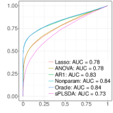
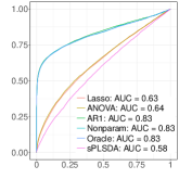
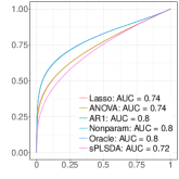
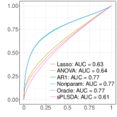
TPR					$\kappa=1$
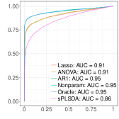
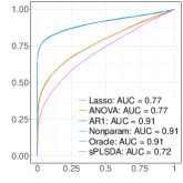
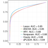
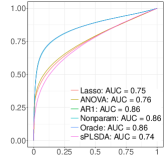
TPR					$\kappa=2$
	FPR

Figure 1. Means of the ROC curves obtained from 200 replications for the different methodologies in the AR(1) dependence modeling; $\kappa$ is linked to the signal to noise ratio (first row: $\kappa=1$, second row $\kappa=2$); $\phi_{1}$ is the correlation level in the AR(1) and $s$ the sparsity level (i.e. the fraction of nonzero elements) in the vector of true parameters.

We can see from Figure 1 that in the case of an AR(1) dependence, taking into account this dependence provides better results than sPLSDA and than approaches that consider the columns of the residual matrix as independent. Moreover, we observe that the performance of the non parametric modeling are on a par with those of the parametric and the oracle ones. We also note that the larger the sparsity level the smaller the difference of performance between the different approaches. However, the larger the signal to noise ratio the better the performance of the different methodologies.

3.2. Choice of the dependence modeling

The goal of this section is to assess the performance of the dependence modeling strategy that we proposed in Section 2.1.3. We generated observations $\boldsymbol{Y}$ with the parameters described at the beginning of Section 3 in the case of an AR(1) dependence, for a sparsity level of 0.01 and when $\kappa=1$. The corresponding results are displayed in Figure 2.

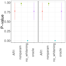
Figure 2. Means and standard deviations of the $p$-values of the test described in Section 2.1.3 for the different approaches in the AR(1) dependence modeling when $\phi_{1}=0.7$ (left) and $\phi_{1}=0.9$ (right).

We observe from this figure that our test provides $p$-values close to zero in the case where no whitening strategy is used (Lasso) and that when one of the proposed whitening approaches is used the $p$-values are larger than 0.7.

3.3. Choice of the model selection criterion

We investigate hereafter the performance of our model selection criterion described in Section 2.2.2.

Figure 3 displays the means of the $p$-values of the test described in 2.1.3 obtained from 5000 replications of the observations $\boldsymbol{Y}$ generated with the parameters described at the beginning of Section 3 in the case of an AR(1) dependence with $\phi_{1}=0.9$ and $\kappa=1$.

Figure 3. Means of the $p$-values associated to the test statistic defined in (10) obtained from 5000 replications when $\kappa=1$.

We observe from this figure that the $p$-values are all the more high that the thresholds are large.

Figure 4 displays with bullets (’$\bullet$’) the positions of the variables selected by our three-step approach for the two possible choices of thresholds from 500 replications of $\boldsymbol{Y}$ obtained with the parameters described at the beginning of Section 3 in the case of an AR(1) dependence with $\phi_{1}=0.9$ and $\kappa=10$.

We observe from this figure that mostly all the positions of the non null variables in $\mathcal{B}$ are retrieved with some false positive when the threshold is obtained by maximizing the $p$-value. When the threshold is equal to 1, there are no false positive but all the true positions are not recovered.

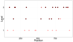
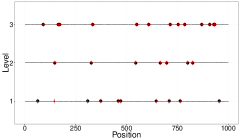
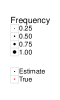
Figure 4. Positions of the variables selected by our approach (’$\bullet$’) when $\kappa=10$. Values on the $y$-axis correspond to the 3 levels of the factor. The results obtained when the threshold is equal to 1 are on the left and the results when the threshold is obtained by maximizing the $p$-value are on the right. The size of the bullets are all the more large that the number of times where a variable has been selected is large.

3.4. Numerical performance

In order to investigate the computational burden of our approach, we generated matrices $\boldsymbol{Y}$ satisfying Model (2) with $n=30$ and $q\in\{100,200,\dots,1000\}$. Here, the rows of the matrix $\boldsymbol{E}$ are generated as realizations of an AR(1) process and the level of sparsity $s$ of $\boldsymbol{B}$ is equal to 0.01.

Figure 5 displays the computational times of MultiVarSel obtained from a computer having the following configuration: RAM 16 GB, CPU $8\times 3.6$ GHz for different number of replications in the stability selection stage. We can see from this figure that the computational burden of MultiVarSel is very low and that it takes only a few seconds to analyze matrices having 1000 columns.

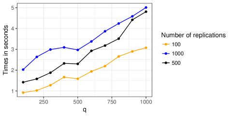
Figure 5. Computational times (in seconds) of MultiVarSel.

4. Application to a LC-MS dataset

In this section, our three-step methodology implemented in the R package MultiVarSel and available from the CRAN, is applied to a LC-MS (Liquid Chromatography-Mass Spectrometry) data set made of African copals samples. The samples correspond to ethanolic extracts of copals produced by trees belonging to two genera Copaifera (C) and Trachylobium (T) with a second level of classification coming from the geographical provenance of the Copaifera samples (West (W) or East (E) Africa). Since all the Trachylobium samples come from East Africa, we have a single factor having three levels: CE, CW and TE such that $n_{\textrm{CE}}=9$, $n_{\textrm{CW}}=8$ and $n_{\textrm{TE}}=13$.

In this section, we also compare the performance of our method with those of other techniques which are widely used in metabolomics.

4.1. Data pre-processing

LC-MS chromatograms were aligned using the R package XCMS proposed by Smith et al. (2006) with the following parameters: a signal to noise ratio threshold of 10:1 for peak selection, a step size of 0.2 min and a minimum difference in m/z for peaks with overlapping retention times of 0.05 amu. Sample filtering was also performed: To be considered as informative, as suggested by Kirwan et al. (2013), a peak was required to be present in at least 80% of the samples. Missing values imputation was realized using the KNN algorithm described in Hrydziuszko and Viant (2012). Subsequently, the spectra were normalized to equalize signal intensities to the median profile in order to reduce any variance arising from differing dilutions of the biological extracts and probabilistic quotient normalization (PQN) was used, see Dieterle et al. (2006) for further details. In order to reduce the size of the data matrix, selection of the adducts of interest [M+H]⁺ was then performed using the CAMERA package of Kuhl et al. (2012). A $n\times q$ matrix $\boldsymbol{Y}$ was then obtained and submitted to the statistical analyses.

4.2. Application of our three-step approach

The observations matrix $\boldsymbol{Y}$ is first centered and scaled in order to ensure that the empirical mean in each column is 0 and that the empirical variance is 1.

4.2.1. First step

A one-way ANOVA is fitted to each column of the observation matrix $\boldsymbol{Y}$ in order to have access to an estimation $\widehat{\boldsymbol{E}}$ of the residual matrix $\boldsymbol{E}$. Then, the test proposed in Section 2.1.3 is applied. We found a $p$-value equal to zero which indicates that the columns of $\widehat{\boldsymbol{E}}$ cannot be considered as independent and hence that applying the whitening strategy should improve the results.

4.2.2. Second step

The different whitening strategies described in Section 2.1 were applied and the highest $p$-value for the test described in Section 2.1.3 is obtained for the nonparametric whitening. More precisely, the $p$-values obtained for the AR(1) and the nonparametric dependence modeling are equal to $1.5\times 10^{-4}$ and 0.5107, respectively. Hence, in the following we shall use the nonparametric modeling.

4.2.3. Third step

The Lasso approach described in Section 2.2 was then applied to the whitened observations where $\widehat{\boldsymbol{\Sigma}}_{q}$ is obtained by using the nonparametric modeling. The stability selection is then used with 5000 replications and a threshold equal to 1 in order to avoid false positive.

The Venn diagram of Figure 6 displays the repartition of the selected metabolites among the different classes CE, TE and CW. We can see from this figure that at least one metabolite is selected as a marker for each class (20 for TE, 22 for CW and 1 for CE) for a total of 39 unique metabolites. More precisely, our methodology leads to a list of metabolites that mainly characterize a single class.

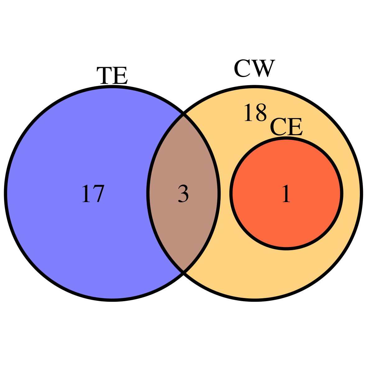
Figure 6. Venn diagram of the metabolites selected for each class by MultiVarSel using a threshold equal to 1 in the stability selection stage.

4.3. Comparison with existing methods

The goal of this section is to compare the performance of our approach with those of methodologies classically used in metabolomics such as partial least square discriminant analysis (PLS-DA) and sparse partial least square discriminant analysis (sPLS-DA) devised by Lê Cao et al. (2011) and implemented in the R package MixOmics.

As recommended by Lê Cao et al. (2011), we used two components for PLS-DA and sPLS-DA. Moreover, in order to make sPLS-DA comparable with our approach, 20 variables are kept for each component in the sPLS-DA methodology. The corresponding results are displayed in Figure 7. We can see from this figure that sPLS-DA exhibits better classification performance than the standard PLS-DA.

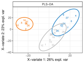
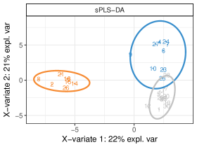
Figure 7. 2D scores plot of the PLS-DA and the sPLS-DA.

Since PLS-DA does not include a variable selection step we shall compare our approach only to sPLS-DA in the following. For comparing these methodologies Figure 8 displays the PCA obtained when all the metabolites are kept on the one hand and when the metabolites are those selected by sPLS-DA or by our methodology on the other hand. We can see from this figure that, one the hand, the approaches containing a variable selection step exhibit better classification performance and that, on the other hand, sPLS-DA and our method show similar performance from the classification point of view even if our approach is not designed for this purpose.

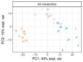
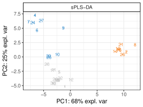
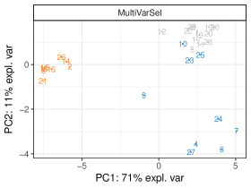
Figure 8. PCA with all the metabolites and with the metabolites selected by sPLS-DA and our approach MultiVarSel.

Figure 9 displays the positions of the metabolites selected by our approach and sPLS-DA. We can see from this figure that out of the 39 selected metabolites, 6 metabolites are selected by both sPLS-DA and our methodology. The major difference between these two variable selection techniques is that our method selects metabolites having a ratio $m/z$ smaller than 300 whereas the metabolites chosen by sPLS-DA lie within the range 300-400 $m/z$.

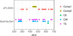
Figure 9. Comparison of the metabolites selected by our approach MultiVarSel and by sPLS-DA.

In order to further compare our methodology with sPLS-DA, we first propose to assess the stability of the selected variables (or metabolites). For this purpose, we performed 10 bootstrap resamplings of our original data and we compared the variables selected by both approaches. The results are displayed in Figure 10 and in Table 1. Figure 10 displays the frequencies at which each metabolite has been selected by the two methods. We can see from this figure that the highest selection frequency of sPLS-DA is around 0.8 and that a lot of variables have a selection frequency smaller than 0.5. Moreover, we can see from Table 1 which provides the number of metabolites which have been selected once (first row), twice (second row)…, that our approach selects 4 metabolites with a frequency equal to 1 which does not occur for sPLS-DA. Hence, from this point of view, our approach is more stable than sPLS-DA.

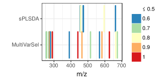
Figure 10. Frequencies of the metabolites selected by sPLS-DA and our approach MultiVarSel.

Nb of selection	Nb of selected metabolites	Nb of selected metabolites
	by sPLS-DA	by MultiVarSel
1	117	143
2	41	54
3	26	24
4	4	20
5	8	15
6	5	6
7	3	6
8	2	3
9	0	3
10	0	4

Table 1. Number of times the different metabolites have been selected by sPLS-DA and our approach MultiVarSel.

Finally, we compare hereafter the set of variables provided by sPLS-DA and our approach from the classification error point of view. Since our method is not designed for yielding a classification we give the selected variables to PLS-DA in order to obtain such a classification. The estimation of the classification error rates are then obtained by using a 10-fold cross-validation. The corresponding results are displayed in Tables 2 and 3. We observe that the classification error rates of our approach are on a par with those of sPLS-DA.

	TE	CE	CW
TE	0.92	0.33	0.00
CE	0.08	0.67	0.00
CW	0.00	0.00	1.00

Table 2. Classification error rates for sPLS-DA.

	TE	CE	CW
TE	0.92	0.22	0.00
CE	0.08	0.67	0.00
CW	0.00	0.11	1.00

Table 3. Classification error rates for our approach coupled with PLS-DA.

We observe from these different investigations that our approach provides similar results as sPLS-DA in terms of classification even if our approach was not designed for this purpose and that it yields more stable variables (metabolites) than sPLS-DA for characterizing the different classes.

5. Conclusion

In this paper, we proposed a novel approach for analyzing LC-MS metabolomics data by introducing a new Lasso-type approach taking into account the dependence that may exist between the columns of the data matrix. Our approach is implemented in the R package MultiVarSel which is available from the The Comprehensive R Archive Network (CRAN). In the course of this study, we have shown that our method has two main features. Firstly, it is very efficient from a statistical point of view for selecting a restricted number of stable metabolites characterizing each level of the factor of interest. Secondly, its very low computational burden makes its use possible on very large LC-MS metabolomics data.

Appendix A

Let $vec(\boldsymbol{A})$ denote the vectorization of the matrix $\boldsymbol{A}$ formed by stacking the columns of $\boldsymbol{A}$ into a single column vector. Let us apply the $vec$ operator to Model (2), then

$$vec(\boldsymbol{Y})=vec(\boldsymbol{X}\boldsymbol{B}+\boldsymbol{E})=vec(\boldsymbol{X}\boldsymbol{B})+vec(\boldsymbol{E}).$$

Let $\mathcal{Y}=vec(\boldsymbol{Y})$, $\mathcal{B}=vec(\boldsymbol{B})$ and $\mathcal{E}=vec(\boldsymbol{E})$. Hence,

$$\mathcal{Y}=vec(\boldsymbol{X}\boldsymbol{B})+\mathcal{E}=(\textrm{I}_{q}\otimes\boldsymbol{X})\mathcal{B}+\mathcal{E},$$

where we used that (Mardia et al., 1979, Appendix A.2.5)

$$vec(AXB)=(B^{\prime}\otimes A)vec(X).$$

In this equation, $B^{\prime}$ denotes the transpose of the matrix $B$. Thus,

$$\mathcal{Y}=\mathcal{X}\mathcal{B}+\mathcal{E},$$

where $\mathcal{X}=\textrm{I}_{q}\otimes\boldsymbol{X}$ and $\mathcal{Y}$, $\mathcal{B}$ and $\mathcal{E}$ are vectors of size $nq$, $pq$ and $nq$, respectively.

Appendix B

Let us apply the $vec$ operator to Model (4) where $\boldsymbol{\Sigma}_{q}^{-1/2}$ is replaced by $\widehat{\boldsymbol{\Sigma}}_{q}^{-1/2}$, then

$$vec(\boldsymbol{Y}\widehat{\boldsymbol{\Sigma}}_{q}^{-1/2})=vec(\boldsymbol{X}\boldsymbol{B}\widehat{\boldsymbol{\Sigma}}_{q}^{-1/2})+vec(\boldsymbol{E}\widehat{\boldsymbol{\Sigma}}_{q}^{-1/2})\\ =((\widehat{\boldsymbol{\Sigma}}_{q}^{-1/2})^{\prime}\otimes\boldsymbol{X})vec(\boldsymbol{B})+vec(\boldsymbol{E}\widehat{\boldsymbol{\Sigma}}_{q}^{-1/2}).$$

Hence,

$${\mathcal{Y}}={\mathcal{X}}\mathcal{B}+{\mathcal{E}},$$

where ${\mathcal{Y}}=vec(\boldsymbol{Y}\widehat{\boldsymbol{\Sigma}}_{q}^{-1/2})$, ${\mathcal{X}}=(\widehat{\boldsymbol{\Sigma}}_{q}^{-1/2})^{\prime}\otimes\boldsymbol{X}$ and ${\mathcal{E}}=vec(\boldsymbol{E}\widehat{\boldsymbol{\Sigma}}_{q}^{-1/2})$.

References

- Boccard and Rudaz (2016) Boccard, J. and S. Rudaz (2016). Exploring omics data from designed experiments using analysis of variance multiblock orthogonal partial least squares. Analytica Chimica Acta 920, 18 – 28.
- Brockwell and Davis (1991) Brockwell, P. and R. Davis (1991). Time Series: Theory and Methods. Springer Series in Statistics. Springer-Verlag New York.
- Dieterle et al. (2006) Dieterle, F., A. Ross, G. Schlotterbeck, and H. Senn (2006). Probabilistic quotient normalization as robust method to account for dilution of complex biological mixtures. application in 1h nmr metabonomics. Analytical Chemistry 78(13), 4281–4290.
- Faraway (2004) Faraway, J. J. (2004). Linear Models with R. Chapman & Hall/CRC.
- Grissa et al. (2016) Grissa, D., M. Petera, M. Brandolini, A. Napoli, B. Comte, and E. Pujos-Guillot (2016). Feature selection methods for early predictive biomarker discovery using untargeted metabolomic data. Frontiers in Molecular Biosciences 3(30).
- Hrydziuszko and Viant (2012) Hrydziuszko, O. and M. R. Viant (2012). Missing values in mass spectrometry based metabolomics: an undervalued step in the data processing pipeline. Metabolomics 8(1), 161–174.
- Kirwan et al. (2013) Kirwan, J., D. Broadhurst, R. Davidson, and M. Viant (2013). Characterising and correcting batch variation in an automated direct infusion mass spectrometry (dims) metabolomics workflow. Analytical and Bioanalytical Chemistry 405(15), 5147–5157.
- Kuhl et al. (2012) Kuhl, C., R. Tautenhahn, C. Boettcher, T. R. Larson, and S. Neumann (2012). Camera: an integrated strategy for compound spectra extraction and annotation of liquid chromatography/mass spectrometry data sets. Analytical Chemistry 84, 283–289.
- Lê Cao et al. (2011) Lê Cao, K.-A., S. Boitard, and P. Besse (2011). Sparse pls discriminant analysis: biologically relevant feature selection and graphical displays for multiclass problems. BMC Bioinformatics 12(1), 253.
- Mardia et al. (1979) Mardia, K., J. Kent, and J. Bibby (1979). Multivariate analysis. Probability and mathematical statistics. Academic Press.
- Meinshausen and Buhlmann (2010) Meinshausen, N. and P. Buhlmann (2010). Stability selection. Journal of the Royal Statistical Society 72(4), 417–473.
- Nicholson et al. (1999) Nicholson, J. K., J. C. Lindon, and E. Holmes (1999). ’metabonomics’: understanding the metabolic responses of living systems to pathophysiological stimuli via multivariate statistical analysis of biological nmr spectroscopic data. Xenobiotica 29(11), 1181–1189. PMID: 10598751.
- Ren et al. (2015) Ren, S., A. A. Hinzman, E. L. Kang, R. D. Szczesniak, and L. J. Lu (2015). Computational and statistical analysis of metabolomics data. Metabolomics 11(6), 1492–1513.
- Rothman et al. (2010) Rothman, A. J., E. Levina, and J. Zhu (2010). Sparse multivariate regression with covariance estimation. Journal of Computational and Graphical Statistics 19(4), 947–962.
- Saccenti et al. (2013) Saccenti, E., H. C. J. Hoefsloot, A. K. Smilde, J. A. Westerhuis, and M. M. W. B. Hendriks (2013). Reflections on univariate and multivariate analysis of metabolomics data. Metabolomics 10(3), 361–374.
- Smith et al. (2006) Smith, C., E. Want, G. O’Maille, R. Abagyan, and G. Siuzdak (2006, Feb 1). XCMS: Processing mass spectrometry data for metabolite profiling using Nonlinear peak alignment, matching, and identification. Analytical Chemistry 78(3), 779–787.
- Tibshirani (1996) Tibshirani, R. (1996). Regression shrinkage and selection via the Lasso. J. Royal. Statist. Soc B. 58(1), 267–288.
- Verdegem et al. (2016) Verdegem, D., D. Lambrechts, P. Carmeliet, and B. Ghesquière (2016). Improved metabolite identification with midas and magma through ms/ms spectral dataset-driven parameter optimization. Metabolomics 12(6), 1–16.
- Zhang et al. (2012) Zhang, A., H. Sun, P. Wang, Y. Han, and X. Wang (2012). Modern analytical techniques in metabolomics analysis. Analyst 137, 293–300.