Light Clusters and Pasta Phases in Warm and Dense Nuclear Matter

Abstract

The pasta phases are calculated for warm stellar matter in a framework of relativistic mean-field models, including the possibility of light cluster formation. Results from three different semiclassical approaches are compared with a quantum statistical calculation. Light clusters are considered as point-like particles, and their abundances are determined from the minimization of the free energy. The couplings of the light-clusters to mesons are determined from experimental chemical equilibrium constants and many-body quantum statistical calculations. The effect of these light clusters on the chemical potentials is also discussed. It is shown that including heavy clusters, light clusters are present until larger nucleonic densities, although with smaller mass fractions.

I Introduction

Presently, there is an increasing interest in the properties of warm and dense matter in astrophysics and heavy ion physics, i.e. nuclear/stellar matter at subsaturation densities (baryon density $n_{B}\leq 0.15$ fm^-3) and moderate temperatures ($T\leq 20$ MeV). Light clusters seem to have an important role in the evolution of core-collapse supernovae arcones08 , affecting in a non-negligible way the average energy of the electron anti-neutrinos. Also, in Refs. furusawa13 ; furusawa16 , it was shown that light clusters may influence in a favorable or unfavorable way, depending on the conditions, the shock revival in the post-bounce phase of core-collapse supernovae.

The determination of light cluster abundances in warm and dense nuclear matter has been investigated using different approaches. Recently, the formation of light clusters in low-density nuclear matter, produced by heavy ion collisions (HIC), has been measured in the laboratory hagel12 ; qin12 , allowing the determination of quantities, such as in-medium binding energies and chemical equilibrium constants. These and further laboratory experiments give a strong evidence that in-medium corrections are relevant for light clusters in nuclear matter at those densities and temperatures. To obtain the corresponding nuclear equation of state (EOS), a correct description of few-body correlations is essential.

The properties of warm dense matter are described by EOSs. In particular, for given constraints, such as the temperature, $T$, and the number of neutrons and protons (densities $n_{n},\,\,n_{p}$, respectively), an ensemble in thermodynamic equilibrium, characterized by a thermodynamic potential, here the free energy, can be defined. In stellar matter, allowing for weak interaction processes, $\beta$-equilibrium is established, and only the baryon number (density $n_{B}=n_{n}+n_{p}$) can be chosen freely. Other equations of state (thermodynamic, caloric, chemical potential, etc.) are derived from the thermodynamic potential in a consistent manner.

Microscopically, the EOS can be derived within many-particle theory if the interaction is known. However, approximations have to be performed, and even the nucleon-nucleon interaction is not fully known, in particular, in dense matter. In the Brueckner approach, the nucleons in dense matter are considered as quasiparticle states with momentum-dependent energy shifts bhf . In an alternative and simpler approach, the medium effects are introduced as semiempirical density functionals. Well-known examples are the mean field approaches, like the Skyrme parametrization walecka ; shf or the relativistic mean-field (RMF) models walecka ; rmf ; fsu ; typel10 , which are fitted to reproduce the properties near the saturation density, see dutra1 and dutra2 for recent compilations of Skyrme interactions and RMF models, respectively. As an important result, these mean-field approaches predict a phase transition in nuclear matter for sufficiently large proton fractions, $Y_{p}=n_{p}/n_{B}$. Taking the Coulomb interaction into account, droplet formation (large nuclei), pasta structures, etc., are obtained, see, for instance, Ref. PCP15 and further references given there.

A drawback of a mean-field approach is that correlations are not directly described, in particular, the formation of bound states. Correlations become of importance at low temperatures and low densities. In the nuclear statistical equilibrium (NSE) model, bound states (nuclei) are considered as new components in addition to neutrons and protons, and reactions bring the distributions of the respective components to thermodynamic equilibrium as described by a mass action law. The picture of an ideal mixture of components, which occasionally can react if they collide, becomes, however, invalid for baryon densities of the order of $10^{-3}$ fm^-3, or larger when mean-field modifications and the Pauli blocking are relevant. In particular, Pauli blocking suppresses the formation of light clusters, and at the Mott density, the clusters are dissolved RMS .

A quantum statistical (QS) approach can describe quantum correlations in a systematic way. For instance, two-nucleon correlations and the in-medium formation of deuteron and scattering phase shifts are given in SRS . The $\alpha$-like correlations are of particular interest because of the relatively large binding energy of the $\alpha$ particle. A quasiparticle concept can be worked out to describe the light clusters ($d\equiv\,^{2}$H,$\,\,t\equiv\,^{3}$H, $\,\,h\equiv\,^{3}$He,$\,\,\alpha\equiv\,^{4}$He) with binding energies which depend not only on the center-of-mass momentum $\bf P$ relative to the medium, but also on the parameters $T,n_{B},Y_{p}$ characterizing the medium roepke15 .

The light-nuclei quasiparticle approach has to take into account also the contribution of the continuum to reproduce the correct virial expansion for the thermodynamic quantities. Another problem exists when the spectral function, corresponding to the respective few-nucleon correlation function, shows no well developed peak structure so that the introduction of the quasiparticle approach becomes no longer well-defined. This occurs, for instance, when the formation of larger clusters becomes relevant which leads to a background contribution to the spectral function, but also at densities close to the saturation density, where the few-nucleon correlations are already implemented in the mean-field contributions. The Mott effect reduces the contribution of light clusters so that a RMF approach is more adequate. More serious is the inclusion of larger clusters. Here, the QS description becomes too complex, and the replacement by semiempirical approaches, such as the Thomas-Fermi model, is necessary to get the correct physics.

It is one goal of the present work to discuss the combination of light cluster approaches with pasta structure concepts. Light clusters (few-nucleon correlations) dominate at low densities and higher temperatures. In this density region of the phase diagram, the light clusters determine the properties of nuclear matter. However, the inclusion of larger clusters using mean-field concepts is important if going to high densities, and a combination of both approaches is of interest. The combination of these light and heavy clusters has also been recently discussed in Ref. pais16 , where the authors used two different approaches, a generalized relativistic density functional and a statistical model with an excluded-volume mechanism, to compare the formation and dissolution of these aggregates in neutron star matter. Thus, in this work, we focus on two questions: Are the chemical equilibrium constants, as derived from the abundances of light clusters, modified if the formation of droplets and pasta-like structures is taken into account? How are the chemical potentials, calculated in a mean-field approach for stellar matter with account of pasta-like structures, influenced if few-body correlations such as formation of light clusters are considered?

To combine QS calculations with RMF concepts, in recent works the light clusters are included in a generalized RMF approach as additional degrees of freedom PCP15 ; typel10 ; ferreira12 . In particular, the effects of including light clusters in nuclear matter and the densities at which the transition between pasta configurations and uniform matter occur are investigated in PCP15 . As claimed there, more realistic parametrizations for the couplings of the light clusters should be implemented. The present work is aimed to contribute to this issue. For instance, the results obtained at low temperatures ($T=5,10$ MeV) and low densities ($n_{B}\approx 10^{-3}$ fm^-3) will be discussed. The goal is to find more precise data in this region.

The discussion about the necessity of including medium effects in the EOS with the contribution of light clusters has emerged when the chemical equilibrium constants (EC) were measured in heavy ion reactions qin12 . Definitively the nuclear statistical equilibrium (NSE) neglecting all in-medium effects was discarded. In addition to the QS approach to describe the chemical constants, the semiempirical excluded volume concept has been worked out further hempel2015 . Satisfactory agreement of excluded volume calculations with the QS method and the experimental data was found. In the present work, the approach which includes light clusters, as well as pasta phases, will be applied to the measured data for the chemical constants.

This paper is organized as follows. In Sec. II, we present the formalism for the calculation of matter including light clusters and pasta phases within a RMF approach. In Sec. III, some results are shown, and a comparison with experimental and QS results is made. Finally, in Sec. IV, a few conclusions are drawn.

II The Formalism

In this section, we summarize the formalism that is used in this work. In particular, we review the RMF Lagrangian density, we discuss the way the cluster-meson couplings are fixed, and we present the density functional approach that has been applied to describe the pasta phases.

II.1 Lagrangian

We describe matter at subsaturation densities formed by protons, neutrons and light clusters within a relativistic mean-field formalism typel10 . These particles interact through an isoscalar-scalar field $\phi$ with mass $m_{s}$, an isoscalar-vector field $V^{\mu}$ with mass $m_{v}$, and an isovector-vector field $\mathbf{b}^{\mu}$ with mass $m_{\rho}$. The light clusters included in the calculation are the bosonic $\alpha$-particles and deuterons $d$, and the fermionic particles tritons ³H, represented by $t$, and helions ³He, represented by $h$. A system of electrons with mass $m_{e}$ is also considered to make matter neutral. The Lagrangian density of the system reads:

$$\mathcal{L}=\sum_{j=n,p,t,h}\mathcal{L}_{j}+\mathcal{L}_{{\alpha}}+\mathcal{L}_{d}+\mathcal{\,L}_{{\sigma}}+\mathcal{L}_{{\omega}}+\mathcal{L}_{{\rho}}$$

$$+\mathcal{L}_{\omega\rho}+\mathcal{L}_{e}+\mathcal{L}_{A}.$$ (1)

where the term $\mathcal{L}_{j}$ is given by

$$\mathcal{L}_{j}=\bar{\psi}_{j}\left[\gamma_{\mu}iD^{\mu}_{j}-M^{*}_{j}\right]\psi_{j},$$ (2)

and the $\alpha$ particles and the deuterons are described as in typel10 , with $\mathcal{L}_{{\alpha}}$ and $\mathcal{L}_{d}$ given, respectively, by

$$\mathcal{L}_{\alpha}=\frac{1}{2}(iD^{\mu}_{\alpha}\phi_{\alpha})^{*}(iD_{\mu\alpha}\phi_{\alpha})-\frac{1}{2}\phi_{\alpha}^{*}{M^{*}_{\alpha}}^{2}\phi_{\alpha},$$ (3)

and

$$\mathcal{L}_{d}=\frac{1}{4}(iD^{\mu}_{d}\phi^{\nu}_{d}-iD^{\nu}_{d}\phi^{\mu}_{d})^{*}(iD_{d\mu}\phi_{d\nu}-iD_{d\nu}\phi_{d\mu})$$

$$-\frac{1}{2}\phi^{\mu*}_{d}{M^{*}_{d}}^{2}\phi_{d\mu},$$ (4)

with

$$iD^{\mu}_{j} = i\partial^{\mu}-g_{vj}V^{\mu}-g_{\rho j}{\boldsymbol{t}}\cdot\mathbf{b}^{\mu}-q_{ei}A^{\mu},$$ (5)

$j=n,p,t,h,\alpha,d$, where $\boldsymbol{t}$ stands for the isospin operator, $M^{*}_{i}$ is the effective mass, $g_{vi}$, and $g_{\rho i}$ are the particle $i$-meson couplings, and $q_{ei}$ is the electric charge of particle $i$. They are defined in the next section.

The meson and photon contributions in eq. (1) are given by

$$\mathcal{L}_{{\sigma}} = \frac{1}{2}\left(\partial_{\mu}\phi\partial^{\mu}\phi-m_{s}^{2}\phi^{2}-\frac{1}{3}\kappa\phi^{3}-\frac{1}{12}\lambda\phi^{4}\right)$$ (6)

$$\mathcal{L}_{{\omega}} = \frac{1}{2}\left(-\frac{1}{2}\Omega_{\mu\nu}\Omega^{\mu\nu}+m_{v}^{2}V_{\mu}V^{\mu}+\frac{1}{12}\xi g_{v}^{4}(V_{\mu}V^{\mu})^{2}\right)$$ (7)

$$\mathcal{L}_{{\rho}} = \frac{1}{2}\left(-\frac{1}{2}\mathbf{B}_{\mu\nu}\cdot\mathbf{B}^{\mu\nu}+m_{\rho}^{2}\mathbf{b}_{\mu}\cdot\mathbf{b}^{\mu}\right)$$ (8)

$$\mathcal{L}_{\omega\rho} = \Lambda_{v}g_{v}^{2}g_{\rho}^{2}V_{\mu}V^{\mu}\mathbf{b}_{\mu}\cdot\mathbf{b}^{\mu}$$ (9)

$$\mathcal{L}_{A} = -\frac{1}{4}F_{\mu\nu}F^{\mu\nu}~{},$$ (10)

where $\Omega_{\mu\nu}=\partial_{\mu}V_{\nu}-\partial_{\nu}V_{\mu}$, $\mathbf{B}_{\mu\nu}=\partial_{\mu}\mathbf{b}_{\nu}-\partial_{\nu}\mathbf{b}_{\mu}-g_{\rho}(\mathbf{b}_{\mu}\times\mathbf{b}_{\nu})$ and $F_{\mu\nu}=\partial_{\mu}A_{\nu}-\partial_{\nu}A_{\mu}$.

Electrons will be included in stellar matter, with the electron Lagrangian density given by

$$\mathcal{L}_{e}=\bar{\psi}_{e}\left[\gamma_{\mu}\left(i\partial^{\mu}+eA^{\mu}\right)-m_{e}\right]\psi_{e}.$$ (11)

The parameters $\kappa$, $\lambda$ and $\xi$ are self-interacting couplings and the $\omega-\rho$ coupling $\Lambda_{v}$ is included to soften the density dependence of the symmetry energy above saturation density. In the present study, we always consider the FSU model fsu . Values for the parameters $\kappa$, $\lambda$ and $\xi$, but also for the coupling constants and the masses of the mesonic components, are given in Refs. fsu ; ferreira12 . The contribution of the hadronic components are discussed in the following section.

II.2 Medium modified masses of the hadronic components

The treatment of warm and dense nuclear matter, including light cluster and pasta phases, demands the appropriate treatment of nucleons in a dense medium. Different approaches are possible, and have been extensively investigated for the single nucleon ($n,p$) contribution. Within a QS approach, a spectral function can be deduced. Then, the quasiparticle concept may be introduced, where the energies of the nucleons are shifted because of medium effects. Note, however, that heavy clusters have never been included in this approach, and will not be considered in the present study. Results of microscopic calculations, such as Brueckner (DBHF) calculations, can be represented by RMF models, which contain parameters adapted to known data, e.g. the properties of nuclei and nuclear matter near the saturation density.

For the single nucleon contribution, within the RMF approach, we have the density-dependent effective mass

$$M^{*}_{j} = M^{*}=M-g_{s}\phi,\quad j=n,p.$$ (12)

We consider the same mass for protons and neutrons in the spirit of the RMF model proposed by Walecka walecka . We do not expect that for the present calculation at finite temperature and large proton fractions this approximation has a noticeable effect. However, for subsaturation cold stellar matter in $\beta$-equilibrium, finite effects may be expected and the experimental masses should be adopted, which may be done in a straightforward manner. Together with (5), the quasiparticle shift of the nucleons is described within the RMF approach. From a more general point of view, the RMF approach used to describe warm and dense matter can be seen as an effective field theory built in the framework of a density functional theory, where the many-body effects are included in the parameters of the model.

The inclusion of correlations, in particular the formation of light clusters, is a delicate problem in the RMF approach. The calculation of the few-body spectral function from which in-medium correlations, in particular bound state formation, are derived, is subject of a QS approach. In full analogy to the concept of single-nucleon quasiparticles, bound states which appear as poles of the few-body spectral functions, can be considered as quasiparticles, with medium-modified energies.

Within the QS approach, this medium modification of the binding energy of nuclei has two reasons. Firstly, the self-energy shift of the constituting nucleons gives a shift of the quasiparticle energy of clusters which is treated in the same manner as the quasiparticle shift of single-nucleon quasiparticles. Secondly, the Pauli blocking due to the surrounding medium produces a shift of the binding energy which, in contrast to the single-nucleon quasiparticle shift, is strongly dependent on temperature and center-of-mass momentum of the bound state. The strong decrease of the binding energy of nuclei, because of Pauli blocking, leads to the dissolution of light clusters already at low nucleon densities. However, the disappearance of bound states with increasing density is not an abrupt change of the properties because the bound states with large c.o.m. momentum can survive up to higher densities, so that the correlations representative for light clusters are present also at higher densities and only smoothly disappear.

Similar to the single-nucleon quasiparticles $\{n,p\}$, the light-cluster quasiparticles $\{d,t,h,\alpha\}$ are considered as additional degrees of freedom in the Lagrangian (1). The coupling of clusters to the meson fields should reproduce the shift of the corresponding quasiparticle energies. We have in the low-density limit, where Pauli blocking effects can be neglected,

$$M^{*}_{i} = M_{0i}-g_{si}\phi,$$ (13)

$$M_{0i} = A_{i}M-B_{0i},\quad i=d,t,h,\alpha,$$ (14)

where $B_{0i}$ are the binding energies of the particles in the vacuum, $B_{0d}=2.224$ MeV, $B_{0t}=8.482$ MeV, $B_{0h}=7.718$ MeV, and $B_{0\alpha}=28.296$ MeV. For the average vacuum nucleon mass, we take the value $M=939$ MeV.

To include the Pauli blocking shift roepke11 ; typel10 , dependent on the c.o.m. momentum, temperature and density, we improve previous approaches ferreira12 ; PCP15 . As in the case of the nucleons $\{n,p\}$, where the coupling constants are fitted to describe known properties of nuclei and nuclear matter, we need experimental data or first principles theoretical calculations to determine the cluster-meson coupling parameters. Results for the properties of nuclear matter at low densities are still missing. A benchmark is obtained from the virial expansions SRS ; HS and an interesting result that gives some information about the medium modifications of light clusters at low densities are the chemical equilibrium constants (EC) which have been calculated in qin12 .

In the present approach, we are going to model medium effects with an appropriate choice of the cluster-meson couplings, where the binding energy of the cluster in the medium is defined by

$$B_{i}=A_{i}M^{*}-M^{*}_{i}.$$ (15)

The couplings are written as $g_{sj}=x_{sj}g_{s}$, $g_{vj}=x_{vj}g_{v}$ and $g_{\rho j}=|Z_{j}-N_{j}|g_{\rho}$, where $A_{j}$ is the mass number, $Z_{j}$ the proton number, and $N_{j}$ the neutron number. The parameters $x_{ij}$ are fixed in the following way: a) $x_{sj}=x_{vj}=1$, for $j=p,n$; b) $x_{si}=\frac{3}{4}A_{i}$, for $i=d,t,h,\alpha$, as proposed in Ref. ferreira12 , because these parameters reproduce quite well the binding energy given in Ref. typel10 , for $T=5$ MeV, and the experimental predictions of the Mott densities at $T=5$ MeV, given in Ref. hagel12 ; c) the parameters $x_{vi}$ are fixed as in ferreira12 , so that the dissolution density at $T=0$ of each type of cluster, defined as the density at which the free energy of clusterized matter equals the free energy of nucleonic matter, is the one obtained in typel10 , where a statistical approach was used. For the FSU fsu EoS, these $x_{vi}$ ratios are given by, see ferreira12 ,

$$\left(\begin{array}[]{c}x_{vd}\\ x_{vt}\\ x_{vh}\\ x_{v\alpha}\end{array}\right)=\left(\begin{array}[]{c}3.516\\ 4.382\\ 4.624\\ 5.675\end{array}\right)\eta$$ (16)

with $\eta=1$. In the present work, we will allow $\eta$ to vary, in order to be able to reproduce the experimental EC. We point out that, in principle, we should consider different values of $\eta$ for the different clusters, but we have avoided this approach to keep the parameter space restricted. We postpone an overall optimization of all the parameters for a future work; d) for the coupling to the $\rho$-meson we consider the simplest approach and take the coupling proportional to the isospin projection of the light cluster. A more realistic choice could be done once the couplings to the $\sigma$ and $\omega$ mesons are more constrained.

Note that the coupling constant, $g_{v}$, describes the repulsive interaction because of Pauli blocking. This is the case for the nucleon-nucleon interaction, where the Pauli blocking acts on the quark substructure of nucleons; it is only weakly dependent on $T$. For the medium shift of the binding energy of light nuclei, also the Pauli blocking is responsible, but because of the different energy scale of the binding energies, the dependence on $T$ is strong. An effective field theory, that takes into account this temperature dependent Pauli blocking effect, will require temperature dependent parameters as implemented in typel10 , and leads to more complex thermodynamics. In the present study, we have kept to constant couplings, and, therefore, the fit we are performing (e.g. $\eta=0.7$) is valid for the temperature region under consideration (5-10 MeV) but cannot be taken from $T=0$ MeV (where $\eta=1$).

II.3 Density functional approach

The calculation of the warm pasta phase, including light clusters, i.e., $\{n,p,d,t,h,\alpha,e\}$ matter, is performed using the numerical prescription given in pasta1 . In this approach, the fields are assumed to vary slowly so that the nucleons and the clusters can be treated as moving in locally constant fields at each point. The finite temperature semiclassical Thomas Fermi (TF) approximation is obtained within a density functional formalism. We start from the grand canonical potential density:

$${\omega} = \omega(\{f_{i+}\},\{f_{i-}\},\{F_{j}\},\{\nabla F_{j}\})$$ (17)

$$= {\cal E}_{t}-T{\cal S}_{t}-\sum_{i=p,n,e,d,t,h,\alpha}\mu_{i}\rho_{i}~{},~{}$$

where $\{f_{i+}\}$, $\{f_{i-}\}$, $i=p,n,e,d,t,h,\alpha$ stand for the proton, neutron, electron, light clusters and respective anti-particle distribution functions, defined in Eq. (26), and $\{F_{j}\}$, $\{\nabla F_{j}\}$ represent the fields $\phi_{0},\,V_{0},\,b_{0},\,A_{0}$ and respective gradients. The quantities ${\cal E}_{t}={\cal E}+{\cal E}_{e}$ and ${\cal S}_{t}={\cal S}+{\cal S}_{e}$ are the total energy and entropy densities, respectively. The total energy density is a functional of the density, and was defined in pasta1 for $T=0$. For finite temperatures, we have a similar expression

$${\cal E}_{t}=\sum_{i=p,n,e,d,t,h,\alpha}E_{i}(\mathbf{r})+g_{v}V_{0}(\mathbf{r})\rho_{v}(\mathbf{r})+g_{\rho}b_{0}(\mathbf{r})\rho_{3}(\mathbf{r})$$

$$+\frac{1}{2}\left[(\nabla\phi_{0}(\mathbf{r}))^{2}+m_{s}^{2}\phi_{0}^{2}(\mathbf{r})\right]+\frac{\kappa}{3!}\phi_{0}^{3}(\mathbf{r})+\frac{\lambda}{4!}\phi_{0}^{4}(\mathbf{r})$$

$$-\frac{1}{2}\left[(\nabla V_{0}(\mathbf{r}))^{2}+m_{v}^{2}V_{0}^{2}(\mathbf{r})+\frac{\xi g_{v}^{4}}{12}V_{0}^{4}(\mathbf{r})\right]$$

$$-\frac{1}{2}\left[(\nabla b_{0}(\mathbf{r}))^{2}+m_{\rho}^{2}b_{0}^{2}(\mathbf{r})\right]-\Lambda_{v}\,g_{v}^{2}\,V_{0}^{2}(\mathbf{r})\,g_{\rho}^{2}\,b_{0}^{2}(\mathbf{r})$$ (18)

$$-\frac{1}{2}\left[\nabla A_{0}(\mathbf{r})\right]^{2}+e\rho_{q}(\mathbf{r})A_{0}(\mathbf{r})~{}~{},$$ (19)

where

$$E_{i}= \frac{\gamma_{i}}{2\pi^{2}}\int dp\,p^{2}\sqrt{p^{2}+{M_{i}^{*}(\mathbf{r})}^{2}}\left(f_{i+}(\mathbf{r},\mathbf{p})+f_{i-}(\mathbf{r},\mathbf{p})\right),$$ (20)

$$i=p,n,d,h,t,\alpha~{}~{},$$

with $\gamma_{i}=2s_{i}+1$, the spin degeneracy of particle $i$, and

$$E_{e}=\frac{1}{\pi^{2}}\int dp\,p^{2}\sqrt{p^{2}+m_{e}^{2}}\left(f_{e+}(\mathbf{r},\mathbf{p})+f_{e-}(\mathbf{r},\mathbf{p})\right)~{}~{}.$$ (21)

In the above expressions,

$$\rho_{v}{(\mathbf{r})}=\sum_{i=p,n,d,t,h,\alpha}{x_{vi}}\rho_{i}(\mathbf{r}),$$ (22)

$$\rho_{3}{(\mathbf{r})}=\sum_{i=p,n,t,h}t_{3i}\rho_{i}(\mathbf{r}),$$ (23)

and

$$\rho_{q}{(\mathbf{r})}=\sum_{i=p,d,t,h,\alpha}\frac{q_{ei}}{e}\rho_{i}(\mathbf{r}),$$ (24)

with

$$\rho_{i}(r)=\frac{\gamma_{i}}{2\pi^{2}}\int dp\,p^{2}\left(f_{i+}(\mathbf{r},\mathbf{p})-f_{i-}(\mathbf{r},\mathbf{p})\right)~{}~{},$$ (25)

where the ground-state (equilibrium) distribution functions are defined as

$$f_{i\pm}(\mathbf{r},\mathbf{p}) = \frac{1}{1+\exp\left[{(\epsilon_{i}^{*}(\mathbf{r},\mathbf{p})\mp\nu_{i})/T}\right]}~{},\,i=p,n,t,h,$$

$$f_{i\pm}(\mathbf{r},\mathbf{p}) = \frac{1}{-1+\exp\left[{(\epsilon_{i}^{*}(\mathbf{r},\mathbf{p})\mp\nu_{i})/T}\right]}~{},\,i=d,\alpha,$$

$$f_{e\pm}({\mathbf{r}},{\mathbf{p}})\, = \,\frac{1}{1+\exp[(\epsilon_{e}\mp\mu_{e})/T]},$$ (26)

with $\epsilon_{i}^{*}(\mathbf{r},\mathbf{p})=\sqrt{p^{2}+M_{i}^{*}(\mathbf{r})^{2}}$, $M_{i}^{*}(\mathbf{r})=M-{g_{si}}\phi_{0}(\mathbf{r})$, and $\epsilon_{e}=\sqrt{p^{2}+m_{e}^{2}}$. $\mu_{e}$ is the electron chemical potential, and the nucleons and clusters effective chemical potentials, $\nu_{i},\,i=p,n,d,t,h,\alpha$, are given by:

$$\nu_{i}=\mu_{i}-g_{vi}V_{0}(\mathbf{r})-{g_{\rho i}}~{}t_{3i}~{}b_{0}(\mathbf{r})-q_{ei}A_{0}(\mathbf{r}),$$ (27)

where $\mu_{i}$ and $q_{ei}$ are, respectively, the chemical potential and electric charge of particle $i$, and $t_{3i}$ is the third component of the isospin operator.

For the entropy, we take the one-body entropy density:

$$S_{t} = -\sum_{i=n,p,t,h}\int\frac{d^{3}p}{4\pi^{3}}~{}\left\{f_{i+}(\mathbf{r},\mathbf{p})\ln f_{i+}(\mathbf{r},\mathbf{p})\right.$$

$$\left.+\left[1-f_{i+}(\mathbf{r},\mathbf{p})\right]\ln\left[1-f_{i+}(\mathbf{r},\mathbf{p})\right]+(f_{i+}\leftrightarrow f_{i-})\right\}.$$

$$-\sum_{i=d,\alpha}\int\gamma_{i}\frac{d^{3}p}{(2\pi)^{3}}~{}\left\{f_{i+}(\mathbf{r},\mathbf{p})\ln f_{i+}(\mathbf{r},\mathbf{p})\right.$$

$$\left.-\left[1+f_{i+}(\mathbf{r},\mathbf{p})\right]\ln\left[1+f_{i+}(\mathbf{r},\mathbf{p})\right]+(f_{i+}\leftrightarrow f_{i-})\right\}.$$

The equations of motion for the meson fields (see pasta1 ) follow from the variational conditions:

$$\frac{\delta}{\delta\phi_{0}(\mathbf{r})}\Omega=\frac{\delta}{\delta V_{0}(\mathbf{r})}\Omega=\frac{\delta}{\delta b_{0}(\mathbf{r})}\Omega=\frac{\delta}{\delta A_{0}(\mathbf{r})}\Omega=0~{},$$ (29)

with

$$\Omega=\int_{\rm{V_{WS\,cell}}}d^{3}r\,\,\,\omega(\{f_{i+}\},\{f_{i-}\},\{F_{j}\},\{\nabla F_{j}\}),$$ (30)

where the space integral is over the volume of the Wigner Seitz cell, defined as $V_{WS}=A_{i}/\rho$, and we are using the same notion of Eq. (17). For the temperatures considered in the present work, the bosonic particles, $d$ and $\alpha$, do not condensate, so we have only considered the thermal contributions, and did not include the condensate terms in the above expressions.

The numerical algorithm for the description of the neutral $\{n,p,d,t,h,\alpha,e\}$ matter at finite temperature is a generalization of the formalism presented in silvia10 . The Poisson equation is always solved by using the appropriate Green’s function according to the spatial dimension of interest, and the Klein-Gordon equations are solved by expanding the meson fields in a harmonic oscillator basis with one, two or three dimensions, based on the method proposed in ring . The differential equations are solved using Neumann boundary conditions, and, when necessary, an auxiliary virtual source profile outside the cell, to help convergence. One important source of numerical problems are the Fermi integrals, hence, we have used the accurate and fast algorithm given in Ref. aparicio for their calculations.

III Results

Figure 1: The range of temperatures and densities of the HIC experiment of Qin et al. qin12 .

In the present section, we discuss how the couplings of the light clusters to the vector meson $\omega$ define the behavior of the equilibrium constant $K_{c}$, and the distribution of the cluster fractions. Considering the measured equilibrium constants (EC) qin12 as a condition for the EOS in the low-density region, an optimum value for the parameter $\eta$ is found. We will next calculate the pasta phase, including light clusters, and using the same parametrizations discussed for homogeneous matter. The effect of including the pasta phase on the EC and the proton and neutron chemical potential is also discussed.

III.1 Light clusters

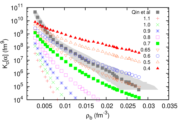
Figure 2: The chemical equilibrium constant $K_{c}$ for the $\alpha$-particle for different values of $\eta$.

In Ref. qin12 , experimentally derived EC for several light clusters ($d,t,h,\alpha$) were reported. The range of densities and temperatures of that experiment is shown in Fig. 1. In the following, we will consider these experimental observables to constrain the cluster coupling to the vector meson $\omega$. The chemical EC defined in qin12 are

$$K_{c}[i]=\frac{\rho_{i}}{\rho_{n}^{N_{i}}\rho_{p}^{Z_{i}}},$$ (31)

where $\rho_{i}$ is the number density of cluster $i$ with neutron number $N_{i}$, and proton number $Z_{i}$, and $\rho_{p}$, $\rho_{n}$ are, respectively, the number densities of free protons and neutrons. The global proton fraction, $Y_{p}=\sum_{i}Z_{i}\rho_{i}/\rho$, with $\rho=\sum_{i}A_{i}\rho_{i}$, was determined in these experiments as $Y_{p}=0.41$.

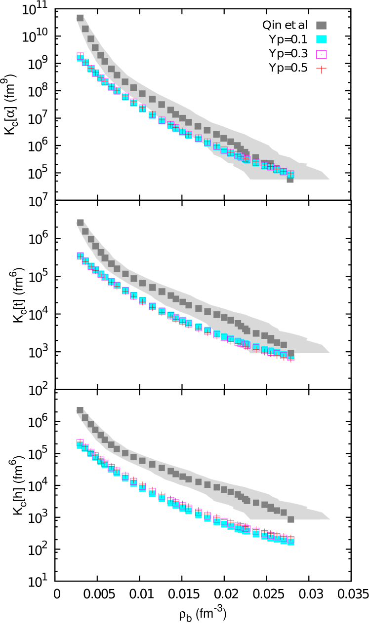
Figure 3: The chemical equilibrium constant $K_{c}$ for the $\alpha$-particle (top), tritium (middle), and helion (bottom) for different global proton fractions values $Y_{p}$, using $\eta=0.65$.

We first consider the EOS for homogeneous matter with light clusters in chemical equilibrium, such that the chemical potential of each cluster is given by

$$\mu_{i}=N_{i}\mu_{n}+Z_{i}\mu_{p}.$$

In our calculation, a gas of protons, neutrons and light clusters is considered in thermodynamical equilibrium. Taking the cluster-meson parametrization proposed in the previous section with the cluster-vector meson couplings defined in (16), we consider $\eta$ a free parameter that will fix the cluster-vector meson coupling. We calculate the $\alpha$-equilibrium constant, $K_{c}[\alpha]$, for different values of $\eta$ and plot them in Fig. 2, together with the experimental results of qin12 . The calculation was performed for $Y_{p}=0.41$. Taking $\eta=1$, the $\alpha$-equilibrium constant is too small, indicating that the parametrization is too repulsive, already for the lowest densities considered. The experimental results seem to indicate that $\eta\sim 0.65-0.7$. In the following, we will consider these two values of $\eta$, and we will discuss the cluster fraction also when heavy clusters are included. In accordance with other models that include the interaction between nucleons and nuclei in the low density region discussed in Refs. qin12 ; hempel2015 , we can reproduce the data obtained from the laboratory test of the EOS. The deviations to the EOS at very low densities, reported also by the other approaches, are possibly caused by the experimental difficulties to produce a state in thermodynamical equilibrium at such densities.

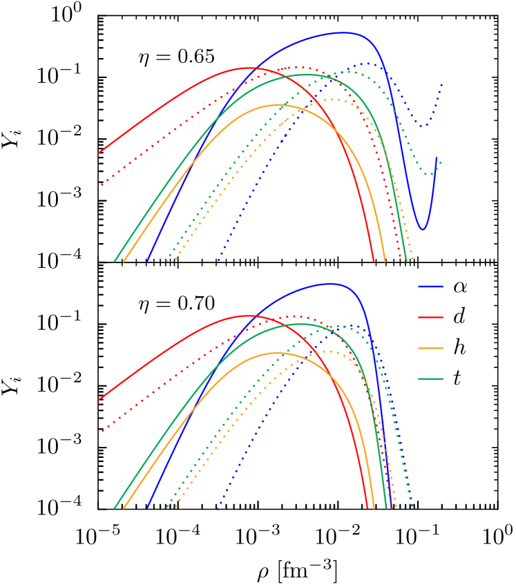
Figure 4: The $i$-cluster particle fraction $Y_{i}$ with $\eta=0.65$ (top panel) and $\eta=0.70$ (bottom panel) for different values of temperature: $5$ MeV (solid), and $10$ MeV (dotted).

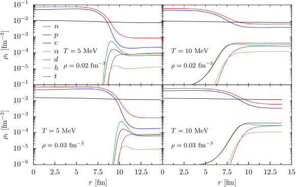
Figure 5: Density profiles for $\eta=0.7$, $Y_{p}=0.41$, $T=5$ MeV (left panels) and $T=10$ MeV (right panels), $\rho=0.02$ fm^-3 (top panels) and $\rho=0.03$ fm^-3 (bottom panels), obtained with the FSU parametrization.

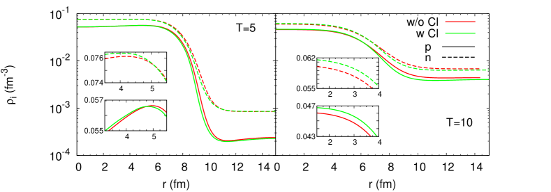
Figure 6: Neutron (dashed) and proton (solid) density profiles for $\eta=0.7$, $Y_{p}=0.41$, and $\rho=0.02$ fm^-3, at $T=5$ (left) and $T=10$ MeV (right panel), obtained for the FSU parametrization, within a TF calculation with (green) and without (red) light clusters.

In the following, we perform our calculations by fixing the proton fraction to $Y_{p}=0.41$, which corresponds to the value extracted from the experiment in Ref. qin12 . However, as seen in Fig. 3, the effect of the total proton fraction on the equilibrium constant of the $\alpha$-particles is very small. It was shown in hempel2015 that for a non-interacting Maxwell-Boltzmann gas of protons, neutrons and clusters in equilibrium, the chemical EC do not depend on the proton fraction. They have, however, obtained a dependence on the proton fraction when describing matter within the excluded volume HS EOS HSB , as a chemical mixture of nuclei and nucleons in nuclear statistical equilibrium, having the density dependent model DD2 typel10 , as the underlying RMF model, and accounting for the Pauli blocking between nucleons and nuclei in a simple approximation by using the excluded volume concept. This difference was attributed to the fact that in their calculation a gas of interacting particles was considered. The observed relative effect in our calculation, although very small, is, however, the same, the smaller the proton fraction, the smaller the EC. The small dependence on $Y_{p}$, close to the ideal gas result, may be explained by the fact that the density distributions depend only on the effective chemical potential, $\nu_{i}$, and the effective masses, which have only the contribution from the coupling to the isoscalar meson field $\sigma$. In the present calculation, we consider a gas of interacting particles, as in Ref. hempel2015 , but in that work, the approach describing the equilibrium, a nuclear statistical equilibrium formalism, is completely different, and this is probably the reason for the different behavior. Contrary to the $\alpha$-clusters, the heliums and tritiums have a non-zero isospin and, therefore, are more sensitive to the global proton fraction of matter, as seen in Fig. 3 in the middle and bottom panels, although the effect of the proton fraction is still quite small. The EC changes in opposite directions since a medium with a smaller proton fraction favors the formation of tritium and disfavors the formation of helium, and so the smaller $Y_{P}$, the larger the tritium EC and the smaller the helium EC.

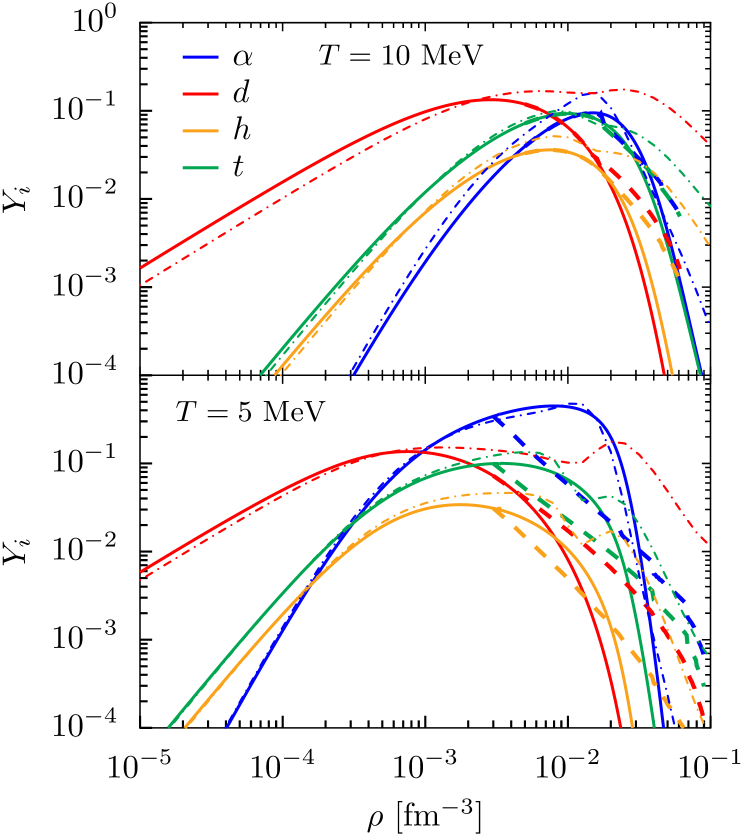
Figure 7: Cluster fractions with $\eta=0.70$ and $Y_{p}=0.41$ as a function of density, for $T=5$ MeV (bottom) and $T=10$ MeV (top panels). Results for a TF calculation (dashed), homogeneous matter with clusters (solid), and the QS approach (dash-dotted lines) are shown. For $T=5$ MeV, the TF calculation includes the five geometrical configurations, droplet, rod, slab, tube and bubble, for the heavy clusters.

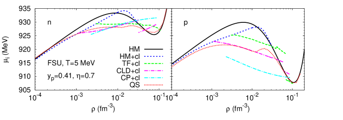
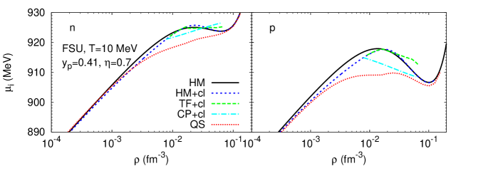
Figure 8: Neutron (left panels) and proton (right panels) chemical potentials with $\eta=0.7$ and $Y_{p}=0.41$ as a function of density at $T=5$ MeV (top) and $T=10$ MeV (bottom), for homogeneous nuclear matter (HM) (solid), nuclear matter with light clusters (blue short-dashed), and mean-field pasta calculations with clusters [TF (green, dashed), CLD (pink, dash-dotted), CP (cyan, dash-dotted)]. QS results (red, dotted) are also shown.

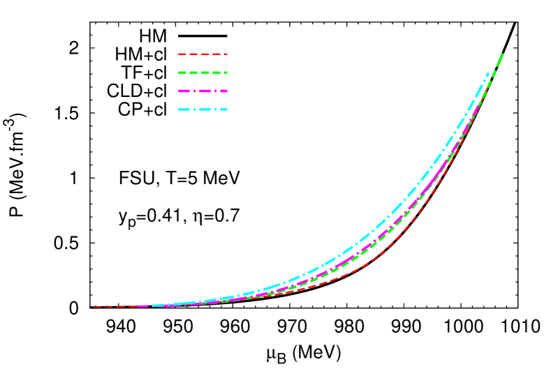
Figure 9: Pressure as a function of the baryonic chemical potential, $\mu_{B}$, at $T=5$ MeV, for homogeneous nuclear matter (HM) (solid), homogeneous nuclear matter with light clusters (red, dashed), and mean-field pasta calculations with clusters [TF (green, dashed), CLD (pink, dash-dotted), CP (cyan, dash-dotted)].

The fractions of the different light clusters present in homogeneous matter with $Y_{p}=0.41$ are plotted in Fig. 4, for $T=5$ and 10 MeV, with $\eta=0.65$ (top panel) and $\eta=0.70$ (bottom panel). Some conclusions are in order: the deuterons are the most abundant clusters at the lowest densities due to their smaller mass. In fact, the relative abundance of the light clusters at the lowest densities is mainly driven by the fugacities $z_{i}=\exp((\mu_{i}-m_{i})/T)\approx z_{n}^{N_{i}}z_{p}^{Z_{i}}$, and, therefore, the lightest cluster is the most abundant at low densities; however, for $T=5$ MeV, the $\alpha$-particles become more abundant, already below $\rho=10^{-3}$fm^-3, due to their large binding energy, and between $\rho=0.01-0.1$ fm^-3, they are the most abundant; the fraction of tritium is always larger than the fraction of helion because matter with $Y_{p}=0.41$ is neutron rich; a larger $\eta$ reduces the fraction of particles and moves the dissolution density to smaller densities as expected, because a larger $\eta$ gives rise to a stronger repulsion, induced by the vector meson; for the largest temperature, and $\eta=0.65$, it is clearly seen that after a strong reduction of the cluster fraction at $\rho<0.1$ fm^-3, there is a new increase of the light cluster fractions, showing that the parametrization of the couplings is not repulsive enough to dissolve the clusters at these densities. This is also seen for the $\alpha$-clusters at $T=5$ MeV. This problem can be fixed by including a mechanism that describes excluded-volume effects, see typel2016 , or by introducing terms beyond a linear dependence on the density in the mass shifts typel10 . In the present calculation, light clusters are considered point-like, and it is the $\omega$-meson that describes the short distance repulsion between clusters, which, however, seems not to be sufficient for these densities. As already mentioned above, the quasiparticle picture becomes questionable near the saturation density, and part of the correlations are already included in the mean-field approach. However, at densities of this order, other effects, such as the formation of heavy clusters, should be considered. This will be done in the next subsection.

III.2 Pasta phase with light clusters

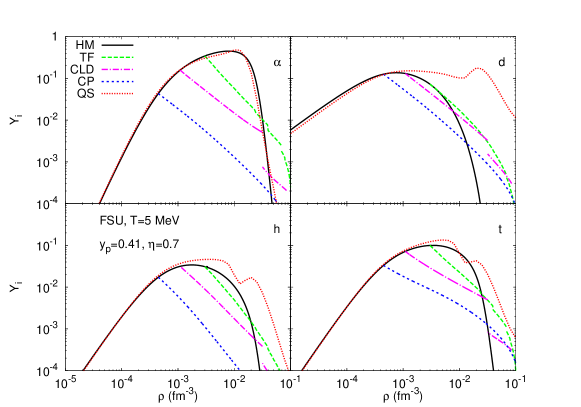
Figure 10: Comparison of the cluster fractions obtained with $\eta=0.70$ as a function of density for $T=5$ MeV: QS calculation (red, dotted lines), three mean-field pasta calculations with clusters, TF (green, dashed), CLD (pink, dash-dotted), CP (blue, short-dashed), and the homogeneous matter (HM) calculation with light clusters (black, solid line).

As seen in Fig. 4, and considering $\eta=0.7$, all the clusters dissolve between $\rho=0.02-0.1$ fm^-3, for the two temperatures considered, $T=5$ and 10 MeV. In the present subsection, we choose this value of $\eta$, and we study how the appearance of heavy clusters is affected by the light clusters. These investigations are of relevance to determine the structure of the inner crust of neutron stars, or the evolution of a core-collapse supernova matter.

We perform a Thomas-Fermi calculation, including light clusters as degrees of freedom, as described in the previous section. We consider the temperatures 5 and 10 MeV, a fixed proton fraction $Y_{p}=0.41$, and the cluster-meson couplings are chosen according to Eq. (16), with $\eta=0.7$. The calculation is performed with the FSU fsu model and all geometrical configurations are considered in the calculation with $T=5$ MeV. For $T=10$ MeV, we only consider droplets because according to reference pethick1998 thermal fluctuations will induce displacements of the rodlike and slablike clusters which can melt the lattice structure for temperatures $T\gtrsim$ 7 MeV.

In Fig. 5, the $p,n,d,t,h$ and $\alpha$-particle profiles for a spherical Wigner-Seitz (WS) cell at the densities $\rho=0.02$ fm^-3 (top panels) and $\rho=0.03$ fm^-3 (bottom panels) are plotted. For $T=5$ MeV, the light clusters present a maximum close to the cluster surface, a result already obtained in typelAIP . Close to the surface, the largest abundances occur for the $\alpha$ and tritium particles, however, at the WS cell border, the deuteron is certainly more abundant than the tritium, and, for $\rho=0.03$ fm^-3, it even overtakes the $\alpha$-particle density. For $T=10$ MeV, the tritium is essentially the most abundant cluster for all densities. The peaked distribution at the heavy cluster surface, observed for $T=5$ MeV, is practically washed out for all light clusters, except for the $\alpha$-particles, when the temperature increases.

In order to study the effect of light clusters on the profiles of the heavy cluster we show, in Fig. 6, the $p$ and $n$ density profiles obtained in a TF calculation with (green) and without (red) light clusters. In the left panel, results at $T=5$ MeV are displayed, and in the right panel, we take $T=10$ MeV, as in the previous Figure. The baryonic density is set at 0.02 fm^-3 and, at this value, the ground state heavy cluster configuration is the droplet, which is the geometry considered in the calculations. The light clusters have a noticeable effect on the heavy cluster, more clearly seen at $T=10$ MeV: including clusters makes the central cluster proton and neutron densities slightly larger, the background gas density of both nucleons lower, the surface thickness of the heavy cluster smaller, and the WS cell radius larger.

Table 1: Transition densities between the heavy clusters within a TF calculation with and without light clusters. The temperature is fixed to $T=5$ MeV and the proton fraction is set to 0.41. In the first column, d, r, s, t, b and HM stand for droplet, rod, slab, tube, bubble and homogeneous matter.

	no clusters		with clusters
	$\rho$ (fm-3)		$\rho$ (fm-3)
d-r	0.0230		0.0234
r-s	0.0392		0.0396
s-t	0.0680		0.0685
t-b	0.0806		0.0790
b-HM	0.101		0.101

In Table 1, we show the sequence of geometries obtained in a TF calculation with and without light clusters, for a temperature of 5 MeV and a fixed proton fraction of 0.41. All the five heavy cluster configurations, droplet, rod, slab, tube and bubble, are present in both calculations and the difference between the transition densities is small, being slightly larger when the light clusters are present, except for the tube-bubble transition, where it happens at a smaller density when no clusters are considered. The small effect of the light clusters on the transitions is probably due to the fact that the largest abundances of clusters occur for densities that favor the spherical geometry, and is below $Y_{i}\sim 0.005$ for all the other geometries which become stable at densities $\rho>0.023$ fm^-3.

In Fig. 7, the fraction of light clusters in homogeneous matter, solid lines, and in the heavy-clusterized matter (pasta phase), dashed lines, are shown. The $T=5$ MeV calculation takes into account the five clusters geometries while for $T=10$ MeV only spherical droplets were considered. Results from a QS approach are also considered (dash-dotted lines), and they will be discussed later. At low densities, the pasta phase calculation converges to the calculation of homogeneous matter with light clusters. This occurs below $\rho=0.001$ fm^-3, for $T=5$ MeV, and below $\rho=0.01$ fm^-3, for the larger temperature. The presence of the pasta clusters has two effects on the light cluster abundances: on one hand, it reduces their abundances for densities between $\rho=0.001-0.01$ fm^-3, close to the light cluster distribution maximum in homogeneous matter, and, on the other hand, it extends their existence to baryonic densities well above the dissolution density of light clusters in homogeneous matter. This behavior can be attributed to the rather small density of the background gas of nucleons in a sizable fraction of the WS cell, where clusters can form abundantly.

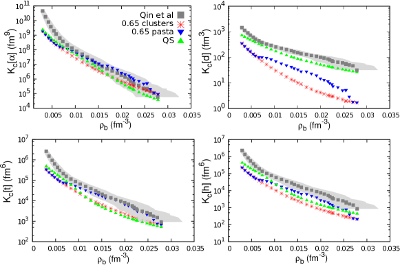
Figure 11: Chemical equilibrium constant $K_{c}$ for $\alpha$-particles (top left), deuterons (top right), tritons (bottom left), and helions (bottom right), and the parameters $\eta=0.65$, $Y_{p}=0.41$, $T$, according to Fig. 1.

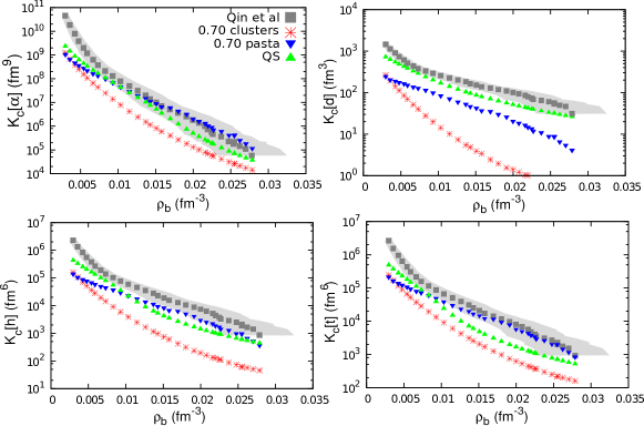
Figure 12: Chemical equilibrium constant $K_{c}$ for $\alpha$-particles (top left), deuterons (top right), tritons (bottom left), and helions (bottom right), and the parameter $\eta=0.70$, $Y_{p}=0.41$, $T$, according to Fig. 1.

The effect of the presence of light clusters on the proton and neutron chemical potentials is seen in Fig. 8. The inclusion of the pasta contribution mainly reduces, or totally removes, the backbending that the proton and neutron chemical potentials show for homogeneous matter with or without light clusters, and that indicates the existence of a chemical instability. The backbending is not totally washed out for the proton chemical potential. However, since the calculation is done at fixed proton fraction including electrons, the chemical potential that determines a possible phase transition is not $\mu_{p}$, but $\mu_{p}+\mu_{e}$ hempel09 , and this one increases continuously with density. Similar results were observed in Ref. PCP15 , where the same FSU model was used, but a different proton fraction, $Y_{p}=0.3$, and temperatures, $T=4$ and 8 MeV, were considered. For comparison, we add to Fig. 8 the results obtained within the coexistence phases (CP) approach, see Ref. PCP15 , and the compressible liquid drop model (CLD) with clusters, see Ref. pais2017 , both calculations including light clusters. In the CP approach, the surface and Coulomb field contributions are added in a non self-consistent calculation, and, therefore, the results should be interpreted with caution. In particular, the approach fails mainly close to the transition between different phases. This drawback is overtaken with the CLD model, and the transition from homogeneous matter with light clusters to pasta phases with light clusters is continuous, see the dash-dotted lines in Fig. 8, the pink for CLD and the cyan for CP models. It is interesting that for $T=5$ MeV, CLD results are very similar to QS results, while TF gives larger chemical potentials. One of the causes of this difference is the fact that in the TF calculation, the electron distribution is determined selfconsistently, while for the CLD model it is a priori taken to be constant.

We are also interested in investigating whether or not a first-order phase transition is occurring in the system. For that purpose, one should look at the pressure-chemical potential graph. This is shown in Fig. 9, where we plot, for the different RMF approaches the pressure as a function of the baryonic chemical potential, $\mu_{B}$, which is defined as $\mu_{B}=(1-y_{p})\mu_{n}+y_{p}(\mu_{p}+\mu_{e})$, because we are considering a fixed proton fraction hempel09 . We include the mean-field pasta calculations with light clusters (TF, dashed green, CLD, dot-dashed pink, and CP, dot-dashed cyan) at $T=5$ MeV. The homogeneous matter results are given by a solid black line, and by a red dashed line, when including light clusters. We observe that the CP shows a jump when the transition to homogeneous matter occurs, which was already discussed in PCP15 and was attributed to the simplified treatment of the surface energy. The other calculations show a smooth transition. We conclude that clusterized matter has a larger pressure at a given density, and, therefore, is more stable than homogeneous matter, and no first order phase transition is expected in these range of densities.

In order to understand how the mean field approach influences the light cluster fraction, we present in Fig. 10 a comparison of the $d,\,t,\,h$ and $\alpha$ fractions, obtained within the five approaches, three mean-field pasta calculation with light clusters (TF, CLD and CP) and two calculation without the pasta structures, QS and mean-field, for $T=5$ MeV. Just comparing the mean-field approaches, we conclude: TF predicts the largest amount of light clusters, although for the deuteron, the CLD model gives similar fractions; the CP model predicts fractions that are 1-2 orders of magnitude smaller; all pasta calculations predict the dissolution of light clusters at larger densities than the calculation without pasta structures; except for the $\alpha$ clusters, the QS calculations predict the largest amounts of light clusters at densities close to 0.1 fm^-3 and above, however this calculation does not consider the possibility of heavy cluster formation. More details about these results will be discussed in the next section. The CLD approach presents some discontinuities that are connected with the change of geometry of the heavy cluster, being a limitation of considering only some geometries and of the single-nucleus approximation. A smoother change would be obtained if, e.g., a full distribution of heavy clusters was considered, and intermediate geometries are taken into account.

III.3 Comparison with other results

In this subsection, we continue to discuss the results of the previous subsections with respect to the experimental data of Ref. qin12 , and compare with the many-body theoretical calculations of Ref. roepke15 . In particular, we are interested in understanding the effect of including the pasta phase in the calculation of the chemical EC and proton and neutron chemical potentials. The experimental chemical EC from qin12 have, however, to be taken with caution due to the uncertainties on the extraction of the density and temperature from an expanding source, since the experimental analysis is performed considering that thermal and chemical equilibrium was attained at the freeze-out point.

III.3.1 Experimental equilibrium constants

Until now, we have focused on the chemical EC for the $\alpha$ particles. Here we discuss also the other light elements ($d$, $t$, $h$). In Figs. 11 and 12, the chemical EC as defined in (31), calculated for homogeneous matter with light clusters (red crosses), and pasta with light clusters (blue triangles) are plotted together with the experimental results of qin12 and the results obtained within a many-body quantum statistical approach roepke15 . It has been discussed in hempel2015 that the comparison with experimental data should be performed only considering light clusters, with $Z\leq 2$, since these particles evaporate from a relatively small source and very small quantities of ⁶Li and ⁷Li are detected. We will consider both the calculation including light clusters in a gas of a homogeneous distribution of protons and neutrons, and in a pasta phase calculation. In this case, the heavy clusters are represented by a single heavy cluster, generally known as single nucleus approximation (SNA).

The curves obtained for the $\alpha$-particle chemical EC for homogeneous matter with light clusters are always below the experimental data, within the uncertainty of the experimental analysis for $\eta=0.65$ or a bit below for $\eta=0.7$, in accordance with Fig. 2. The same trend is obtained for the other three light clusters, $t,\,h,\,$ and $d$. The inclusion of the heavy clusters in the calculation brings the chemical EC closer to the experimental results. A similar effect was shown in hempel2015 for the STOS EOS of Shen et al. stos and the LS EOS of Lattimer and Swesty LS : the EC determined including heavy clusters are larger. As in LS and differing from STOS, our results with the heavy clusters agree with the experimental EC, while the calculation obtained considering only light clusters originates too small EC. We consider that this may be due to the fact that the number of light clusters with respect to the free nucleons for a given density is larger, the larger the different number of cluster species are taken into account. This behavior has been presented in hempel2015 , where, using the EOS of Hempel and Schaffner-Bielich (HS) HSB , the calculation of the EC was carried out considering $np\alpha$ matter, as well as matter with $A\leq 4$, $A\leq 10$ and no restriction on $A$. The larger the number of particles included, the larger the EC obtained.

While the results for the $\alpha$, $t$ and even the $h$ particles are consistent with the experimental results, the deuteron EC are too low, and not even the inclusion of the heavy clusters is enough to reproduce the experimental results. In the present approach, the coupling of mesons to the light clusters mimic the many-body effects that give rise to the formation of clusters. In fact, as discussed in roepke15 , medium modifications due to self-energies and Pauli blocking effects prevent the use of a simple picture that considers the chemical equilibrium of free nuclei. The in-medium effects are included in our mean-field description through an appropriate choice of the coupling constants of the mesons to the light clusters. It is expected that the heavier clusters may be reasonably described, but the smaller the cluster the more important the quantum statistical effects are. Deuterons, being the lightest clusters will, therefore, be more sensitive to the approach and, in order to be realistically described, a more fundamental formalism is required roepke09 ; typel10 ; roepke11 ; roepke15 .

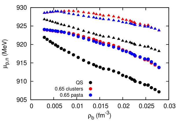
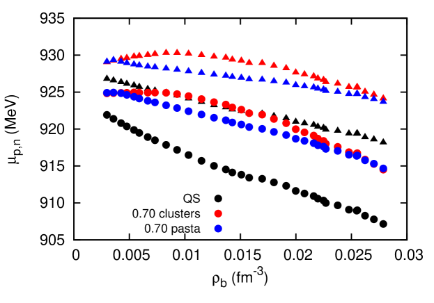
Figure 13: Proton chemical potential, $\mu_{p}$, (circles), and neutron chemical potential, $\mu_{n}$, (triangles), for the parameter $\eta=0.65$ (top), 0.70 (bottom panel), and $Y_{p}=0.41$, for homogeneous matter including light clusters (red), pasta calculation (blue), and the QS approach (black).

III.3.2 Quantum statistical results

In order to compare the predictions of our mean-field approach with the more fundamental many-body quantum statistical (QS) description roepke15 , we have also included in Figs. 7 - 13 the corresponding QS results. It should, however, be stressed that contrary to the RMF approach just discussed, the present QS results do not have the contribution of heavy clusters. Starting with Figs. 11 and 12, we see that the experimental EC data are well described by the QS calculations. Note that small deviations from the results given in hempel2015 are caused by the use of the more recent expressions for the momentum dependent shifts, given in roepke15 . A reasonable agreement with the RMF model, including light cluster formation, is also obtained for the parameter $\eta=0.7$ and the account of pasta formation. A comparison of the cluster fractions, calculated from the different models in a wide density region, is shown in Figs. 7 and 8, where we have plotted, for $\eta=0.7$, the particle fractions at $T=5$ and $10$ MeV, with and without pasta clusters, including also the corresponding results obtained within a QS calculation.

At low densities, in Fig. 7, the particle fractions for the QS and RMF results agree quite well, except for a over production of deuterons in RMF with respect to QS. This difference increases with temperature. The reason is clear: we have to take into account also the continuum contribution SRS ; HS to obtain the correct virial expansion. The contribution of continuum correlations to the EOS roepke15 is increasing with increasing temperature. An approach to combine both, the virial expansion and the RMF theory, was given in VT .

The agreement of both calculations of cluster fractions stops at the maximum of the particle distributions. At larger densities, particle fractions are generally larger within the QS description. In this QS calculation, a momentum dependent Pauli blocking was implemented and the larger the momentum the weaker the Pauli blocking, originating larger mass fractions of light clusters roepke15 . The relatively large contribution of cluster fractions from the QS calculation, especially the two-nucleon correlations ($d$) near the saturation density, is also seen in Fig. 10.

At larger densities, heavy clusters will form and, contrary to the RMF calculation, these have not been considered in the QS calculation. It is precisely at the densities where the momentum dependence of QS Pauli blocking effect is more strongly felt that the heavy clusters appear. The inclusion of the pasta phases postpones the dissolution of light clusters to larger densities but also reduces their relative mass fractions. The RMF calculation includes the backreaction of the light clusters on the mean-field, an effect that is not taken into account in the QS calculation which, therefore, predicts too strong correlations at larger densities. Correlations, in particular two-nucleon correlations, are present in nuclear matter also near the saturation density, but are included in the effective mean field which is fitted to the properties of dense nuclear matter.

In Fig. 8, we include the QS proton and neutron chemical potentials together with the RMF ones. These quantities indicate that the correlations included within each approach are different and stronger in the QS calculation. At low densities, both approaches agree reasonably well, in particular for neutrons. The inclusion of the heavy clusters lowers the chemical potential, becoming closer to the QS values. The backbending effect on the neutron and proton chemical potentials in homogeneous matter with no clusters is the signature of an instability that originates a liquid-gas like phase transition. In the QS approach, this backbending is reduced but not totally removed, and, therefore, the liquid-gas instability is still present, indicating that heavier clusters must be considered, see raduta10 . The RMF pasta phase calculation removes the backbending of the neutron chemical potential, and reduces a lot the backbending effect of the proton chemical potential. The remaining effect is removed by the electron contribution that has also been included in the calculation to neutralize matter.

In Fig. 13, we have plotted the proton and neutron chemical potentials for the densities and temperatures at which the EC are measured. We consider both the RMF results with and without pasta for $\eta=0.65$, $\eta=0.7$, and the QS results. The densities and temperatures tested correspond precisely to the range of densities where the larger discrepancies between the chemical potentials calculated within each framework differ the most. The inclusion of the pasta lowers the chemical potential, as shown before, but the chemical potential still remains essentially 5 MeV larger than the QS results. In contrast to the EC results where both approaches, the RMF as well as the QS approach, reproduce reasonably well the measured data, the results for the chemical potentials $\mu_{n},\mu_{p}$ are quite different. The chemical potentials contain the single-nucleon mean-field shifts which are depending on the RMF parametrization, in our case the FSU model fsu for the pasta calculation including light clusters and the DD2-RMF typel10 used in the QS calculations. Calculating the cluster fractions, these mean-field shifts compensate nearly. Consequently, the EC, see Figs. 11 and 12, show a good agreement between both approaches.

IV Conclusions

In the present study, we have calculated the equation of state at low density, including light clusters with $A\leq 4$ as new degrees of freedom, besides protons and neutrons, within three different RMF calculations: the Thomas-Fermi, the coexistence phase, and the compressible liquid drop models. Results from a quantum statistical calculation were also discussed, for comparison. We have considered two different scenarios: a) the light clusters are in equilibrium with an homogeneous distribution of protons and neutrons; b) the nucleons clusterize and the light clusters coexist with a heavy cluster and a proton-neutron background gas. It has been shown that including heavy clusters shifts the light cluster Mott densities to larger values, although reducing the mass fraction of each type.

The RMF description of light clusters requires a reasonable choice of the cluster-meson couplings. This has been implemented considering both many-body quantum statistical calculations and experimental results from HIC. Compared with the results shown in Ref. PCP15 , the introduction of the parameter $\eta$ which parametrizes the interaction of the meson fields with the light clusters, allows a reasonable description of the measured EC data. With respect to the chemical potentials, $\mu_{n}$ and $\mu_{p}$, larger deviations are obtained, if comparing with QS calculations. These QS calculations will be modified taking the formation of pasta structures into account.

Through the coupling of the light clusters to the mesons, we expect to take into account the backreaction effect of the clusters in the medium, together with an effective description of the in-medium particle self-energies and Pauli blocking effects. For densities below $0.1n_{sat}$, good agreement between the different approaches is obtained for the cluster fractions. However, further studies should be carried out to understand how the many-body effects can be effectively taken into account if the region of higher densities, near the saturation density, is investigated. If attractive correlations are included through too strong couplings, it may occur that light clusters will not dissolve at large densities, and the appropriate treatment of correlations, for instance within a density functional formalism, has to be worked out.

The simultaneous treatment of light clusters and pasta phases in warm and dense nuclear matter is of substantial relevance for various applications in HIC and astrophysics. As an example, we refer to the structure of neutron stars. The clusterization of the background gas in the inner crust has certainly important effects on the transport properties. The fast decrease of the particle fractions just below $0.1$ fm^-3 coincides with the crust-core transition density. The presence of light clusters will affect the neutrino reaction and diffusion processes as well as transport properties, such as electrical conductivity and specific heat. The present work contributes to the investigation of the state of warm and dense matter when in addition to the formation of pasta phases, also light clusters have to be taken into account which require a quantum statistical approach.

References

- (1) A. Arcones, G. Martínez-Pinedo, E. O’Connor, A. Schwenk, H.-Th. Janka, C. J. Horowitz, and K. Langanke, Phys. Rev. C 78, 015806 (2008).
- (2) S. Furusawa, H. Nagakura, K. Sumiyoshi, and S. Yamada, Astrophys. J. 774, 78 (2013).
- (3) S. Furusawa, K. Sumiyoshi, S. Yamada, and H. Suzuki, Nucl. Phys. A 957, 188 (2017).
- (4) L. Qin, K. Hagel, R. Wada, J. B. Natowitz, S. Shlomo, A. Bonasera, G. Röpke, S. Typel, Z. Chen, M. Huang, et al., Phys. Rev. Lett. 108, 172701 (2012).
- (5) K. Hagel et al., Phys. Rev. Lett. 108, 062702 (2012).
- (6) E. N. E. van Dalen and H. Müther, Int. J. Mod. Phys. E 19, 2077 (2010); N. Van Giai, B. V. Carlson, Z. Ma, and H. Wolter, J. Phys. G 37, 064043 (2010); S. Shen, J. Hu, H. Liang, J. Meng, P. Ring, S. Zhang, Chin. Phys. Lett. 33, 102103 (2016).
- (7) A. W. Steiner, M. Prakash, J. M. Lattimer, and P. J. Ellis, Phys. Rep. 411, 325 (2005); L. G. Cao, U. Lombardo, C. W. Shen, and N. Van Giai, Phys. Rev. C 73, 014313 (2006); S. Goriely, N. Chamel, and J. M. Pearson, Phys. Rev. Lett. 102, 152503 (2009); S. Goriely, N. Chamel, and J. M. Pearson, Phys. Rev. C 82, 035804 (2010); J. M. Pearson, N. Chamel, A. F. Fantina, and S. Goriely, Eur. Phys. J. A 50, 43 (2014).
- (8) J. D. Walecka, Ann. Phys. 83, 491 (1974).
- (9) C. J. Horowitz and L. Piekarewicz, Phys. Rev. Lett. 86, 5647 (2001); S. Typel and H. H. Wolter, Nucl. Phys. A 656, 331 (1999); G. A. Lalazissis, T. Nikšić, D. Vretenar, and P. Ring, Phys. Rev. C 71, 024312 (2005); T. Gaitanos, M. Di Toro, S. Typel et al., Nucl. Phys. A 732, 24 (2004); S. K. Dhiman, R. Kumar, and B. K. Agrawal, Phys. Rev. C 76, 045801 (2007).
- (10) B.G. Todd-Rutel and J. Piekarewicz, Phys. Rev. Lett. 95, 122501 (2005).
- (11) S. Typel, G. Röpke, T. Klähn, D. Blaschke, and H. H. Wolter, Phys. Rev. C 81, 015803 (2010).
- (12) M. Dutra, O. Lourenço, J. S. Sá Martins, A. Delfino, J. R. Stone, and P. D. Stevenson Phys. Rev. C 85, 035201 (2012).
- (13) M. Dutra, O. Lourenço, S. S. Avancini, B. V. Carlson, A. Delfino, D. P. Menezes, C. Providência, S. Typel, and J. R. Stone, Phys. Rev. C 90, 055203 (2014).
- (14) H. Pais, S. Chiacchiera, and C. Providência, Phys. Rev. C 91, 055801 (2015).
- (15) G. Röpke, L. Münchow, and H. Schulz, Nucl. Phys. A 379, 536 (1982); Phys. Lett. B 110, 21 (1982).
- (16) M. Schmidt et al., Ann. Phys. 202, 57 (1990).
- (17) G. Röpke, Phys. Rev. C 92, 054001 (2015).
- (18) H. Pais and S. Typel, arXiv:1612.07022 [nucl-th] (2016).
- (19) M. Ferreira and C. Providência, Phys. Rev. C 85, 055811 (2012).
- (20) M. Hempel, K. Hagel, J. Natowitz, G. Röpke, and S. Typel, Phys. Rev. C 91, 045805 (2015).
- (21) G. Röpke, Nucl. Phys. A 867, 66 (2011).
- (22) C. J. Horowitz and A. Schwenk, Nucl. Phys. A 776, 55 (2006).
- (23) S.S. Avancini, D.P. Menezes, M.D. Alloy, J.R. Marinelli, M.M.W. Moraes, and C. Providência, Phys. Rev. C 78, 015802 (2008).
- (24) Sidney S. Avancini, Silvia Chiacchiera, Débora P. Menezes, and Constança Providência, Phys. Rev. C 82, 055807 (2010).
- (25) P. Ring and P. Schuck, The Nuclear Many-Body Problem (Springer, Berlin 1980).
- (26) Josep M. Aparicio, Astrophys. J. Supp. Series 117, 627 (1998).
- (27) M. Hempel and J. Schaffner-Bielich, Nucl. Phys. A 837, 210 (2010).
- (28) S. Typel, Eur. Phys. J. A 52, 16 (2016).
- (29) C. J. Pethick and A. Y. Potekhin, Phys. Lett. B 427, 7 (1998).
- (30) S. Typel, AIP Conf. Proc. 1520, 68 (2013).
- (31) M. Hempel, G. Pagliara, and J. Schaffner-Bielich, Phys. Rev. D 80, 125014 (2009).
- (32) H. Pais, F. Gulminelli, and C. Providência, in preparation (2017).
- (33) H. Shen, H. Toki, K. Oyamatsu, and K. Sumiyoshi, Progr. Theor. Phys. 100, 1013 (1998); Nucl. Phys. A 637, 435 (1998).
- (34) J. M. Lattimer and F. D. Swesty, Nucl. Phys. A 535, 331 (1991).
- (35) G. Röpke, Phys. Rev. C 79, 014002 (2009).
- (36) M. D. Voskresenskaya and S. Typel, Nucl. Phys. A 887, 42 (2012).
- (37) Ad. R. Raduta and F. Gulminelli, Phys. Rev. C 82, 065801 (2010).