Catalyst Acceleration
for Gradient-Based Non-Convex Optimization

Abstract

We introduce a generic scheme to solve nonconvex optimization problems using gradient-based algorithms originally designed for minimizing convex functions. Even though these methods may originally require convexity to operate, the proposed approach allows one to use them on weakly convex objectives, which covers a large class of non-convex functions typically appearing in machine learning and signal processing. In general, the scheme is guaranteed to produce a stationary point with a worst-case efficiency typical of first-order methods, and when the objective turns out to be convex, it automatically accelerates in the sense of Nesterov and achieves near-optimal convergence rate in function values. These properties are achieved without assuming any knowledge about the convexity of the objective, by automatically adapting to the unknown weak convexity constant. We conclude the paper by showing promising experimental results obtained by applying our approach to incremental algorithms such as SVRG and SAGA for sparse matrix factorization and for learning neural networks.

1 Introduction

We consider optimization problems of the form

$$\min_{x\in{\mathbb{R}}^{p}}\>\left\{f(x)\triangleq\frac{1}{n}\sum^{n}_{i=1}f_{i}(x)+\psi(x)\right\}\,.$$ (1)

Here each function $f_{i}\colon{\mathbb{R}}^{p}\to{\mathbb{R}}$ is smooth, the regularization $\psi\colon{\mathbb{R}}^{p}\to\overline{\mathbb{R}}$ may be nonsmooth, and we consider the extended real number system $\overline{\mathbb{R}}:={\mathbb{R}}\cup\{\infty\}$. By considering extended real-valued functions, this composite setting also encompasses constrained minimization by letting $\psi$ be the indicator function of the constraints on $x$. Minimization of regularized empirical risk objectives of form (1) is central in machine learning. Whereas a significant amount of work has been devoted to this composite setting for convex problems, leading in particular to fast incremental algorithms [see, e.g., 16, 27, 33, 50, 53, 55], the question of minimizing efficiently (1) when the functions $f_{i}$ and $\psi$ may be nonconvex is still largely open today.

Yet, nonconvex problems in machine learning are of high interest. For instance, the variable $x$ may represent the parameters of a neural network, where each term $f_{i}(x)$ measures the fit between $x$ and a data point indexed by $i$, or (1) may correspond to a nonconvex matrix factorization problem (see Section 7). Besides, even when the data-fitting functions $f_{i}$ are convex, it is also typical to consider nonconvex regularization functions $\psi$, for example for feature selection in signal processing [23]. In this work, we address two questions from nonconvex optimization:

1. How to apply a method for convex optimization to a nonconvex problem?

2. How to design an algorithm which does not need to know whether the objective function is convex while obtaining the optimal convergence guarantee if the function is convex?

Several works attempted to transfer ideas from the convex world to the nonconvex one, see, e.g., [20, 21]. Our paper has a similar goal and studies the extension of Nesterov’s acceleration for convex problems [36] to nonconvex composite ones. For $C^{1}$-smooth and nonconvex problems, gradient descent is optimal among first-order methods in terms of information based complexity to find an $\varepsilon$-stationary point [10, Theorem 2, Sec. 5]. Without additional assumptions, worst case complexity for first-order methods can not achieve better than $\mathcal{O}(\varepsilon^{-2})$ oracle queries [13, 14]. Under a stronger assumption that the objective function is $C^{2}$-smooth, state-of-the-art methods [e.g., 11] achieve a marginal gain with complexity $O(\varepsilon^{-7/4}\log(1/\varepsilon))$, and do not appear to generalize to composite or finite-sum settings. For this reason, our work fits within a broader stream of recent research on methods that do not perform worse than gradient descent in the nonconvex case (in terms of worst-case complexity), while automatically accelerating for minimizing convex functions. The hope when applying such methods to nonconvex problems is to see acceleration in practice, by heuristically exploiting convexity that is “hidden” in the objective (for instance, local convexity near the optimum, or convexity along the trajectory of iterates).

The main contribution of this paper is a generic meta-algorithm, dubbed 4WD-Catalyst, which is able to use a gradient-based optimization method ${\mathcal{M}}$, originally designed for convex problems, and turn it into an accelerated scheme that also applies to nonconvex objective functions. The proposed 4WD-Catalyst can be seen as a $\bf{4}$-Wheel-Drive extension of Catalyst [31, 32] to all optimization “terrains” (convex and nonconvex). Specifically, without knowing whether the objective function is convex or not, our algorithm takes a method ${\mathcal{M}}$ designed for convex optimization problems with the same structure as (1), e.g., SAGA [16], SVRG [55], and apply ${\mathcal{M}}$ to a sequence of sub-problems such that it asymptotically provides a stationary point of the nonconvex objective. Overall, the number of iterations of ${\mathcal{M}}$ to obtain a gradient norm smaller than $\varepsilon$ is $\tilde{O}(\varepsilon^{-2})$ in the worst case, while automatically reducing to $\tilde{O}(\varepsilon^{-2/3})$ if the function is convex.

Related work.

Inspired by Nesterov’s acceleration method for convex optimization [37], the first accelerated method performing universally well for nonconvex and convex problems was introduced in [20]. Specifically, this work addresses composite problems such as (1) with $n=1$, and, provided the iterates are bounded, it performs no worse than gradient descent on nonconvex instances with complexity $O(\varepsilon^{-2})$ on the gradient norm. When the problem is convex, it accelerates with complexity $O(\varepsilon^{-2/3})$. Extensions to accelerated Gauss-Newton type methods were also recently developed in [17]. In a follow-up work, the authors of [21] proposed a new scheme that monotonically interlaces proximal gradient descent steps and Nesterov’s extrapolation; thereby achieving similar guarantees as [20] but without the need to assume the iterates to be bounded. Extensions when the gradient of $\psi$ is only Hölder continuous can also be devised. Whether accelerated methods are superior to gradient descent remains an open question in the nonconvex setting; their performance escaping saddle points faster than gradient descent has been observed [24, 42].

In [30], a similar strategy is proposed, focusing instead on convergence guarantees under the so-called Kurdyka-Łojasiewicz inequality—a property corresponding to polynomial-like growth of the function, as shown by [8]. Our scheme is in the same spirit as these previous papers, since it monotonically interlaces proximal-point steps (instead of proximal-gradient as in [21]) and extrapolation/acceleration steps. A fundamental difference is that our method is generic and accommodates inexact computations, since we allow the subproblems to be approximately solved by any method we wish to accelerate.

By considering $C^{2}$-smooth nonconvex objective functions $f$ with Lipschitz continuous gradient $\nabla f$ and Hessian $\nabla^{2}f$, the authors of [11] propose an algorithm with complexity $O(\varepsilon^{-7/4}\log(1/\varepsilon))$, based on iteratively solving convex subproblems closely related to the original problem. It is not clear if the complexity of their algorithm improves in the convex setting. Note also that the algorithm proposed in [11] is inherently for $C^{2}$-smooth minimization and requires exact gradient evaluations. This implies that the scheme does not allow incorporating nonsmooth regularizers and can not exploit finite sum structure.

In [46], stochastic methods for minimizing (1) using variants of SVRG [25] and SAGA [16]. Their scheme works for both convex and nonconvex settings and achieves convergence guarantees of $O(Ln/\varepsilon)$ (convex) and $O(n^{2/3}L/\varepsilon^{2})$ (nonconvex). Although for nonconvex problems our scheme guarantees a rate of $\tilde{O}\left(\frac{nL}{\varepsilon^{2}}\right)$, it enjoys the optimal accelerated rate in the convex setting (See Table 1). The empirical results of [46] used a step size of $1/L$, but their theoretical analysis without mini-batching required a much smaller step-size, $1/(n^{2/3}L)$, whereas our analysis is able to use the larger $1/L$ stepsize.

	Theoretical stepsize	Nonconvex	Convex
SVRG [55]	$\displaystyle O\left(\frac{1}{L}\right)$	not avail.	$\displaystyle O\left(n\frac{L}{\varepsilon}\right)$
ncvx-SVRG [3, 45, 46]	$\displaystyle O\left(\frac{1}{n^{2/3}L}\right)$	$\displaystyle O\left(\frac{n^{2/3}L}{\varepsilon^{2}}\right)$	$\displaystyle O\left(\sqrt{n}\frac{L}{\varepsilon}\right)$
4WD-Catalyst -SVRG	$\displaystyle O\left(\frac{1}{L}\right)$	$\displaystyle\tilde{O}\left(\frac{nL}{\varepsilon^{2}}\right)$	$\displaystyle\tilde{O}\left(\sqrt{\frac{nL}{\varepsilon}}\right)$

Table 1: Comparison of rates of convergence when applying 4WD-Catalyst  to SVRG. In the convex case, we present the complexity in terms of number of iterations to obtain a point $x$ satisfying $f(x)-f^{*}<\varepsilon$. In the nonconvex case, we consider instead the guarantee $\text{dist}(0,\partial f(x))<\varepsilon$. Note that the theoretical stepsize of ncvx-SVRG is much smaller than that of our algorithm and of the original SVRG. In practice, the choice of a small stepsize significantly slows down the performance (see Section 7), and ncvx-SVRG is often heuristically used with a larger stepsize in practice, which is not allowed by theory, see [46]. A mini-batch version of SVRG is also proposed there, allowing large stepsizes of $O(1/L)$, but without changing the global complexity. A similar table for SAGA [16], gradient descent, and randomized coordinate descent is provided in Table 2 of Section 6.

A stochastic scheme for minimizing (1) under the nonconvex but smooth setting were recently considered in [29]. The method can be seen as a nonconvex variant of the stochastically controlled stochastic gradient (SCSG) methods [28]. If the target accuracy is small, then the method performs no worse than nonconvex SVRG [46]. If the target accuracy is large, the method achieves a rate better than SGD. The proposed scheme does not incorporate nonsmooth regularizers and it is unclear whether numerically the scheme performs as well as SVRG.

Finally, a stochastic method related to SVRG [25] for minimizing large sums while automatically adapting to the weak convexity constant of the objective function is proposed in [2]. When the weak convexity constant is small (i.e., the function is nearly convex), the proposed method enjoys an improved efficiency estimate. This algorithm, however, does not automatically accelerate for convex problems, in the sense that the overall rate is slower than $O(\varepsilon^{-3/2})$ in terms of target accuracy $\varepsilon$ on the gradient norm.

Organization of the paper.

Section 2 presents mathematical tools for non-convex and non-smooth analysis, which are used throughout the paper. We provide a discussion of related works for solving the nonconvex and nonsmooth problem (1) in Section 3. In Sections 4 and 5, we introduce the main algorithm and important extensions, respectively. Section 6 presents global convergence guarantees of the scheme and convergence guarantees when the algorithm wraps specific algorithms such as SAGA, SVRG, and randomized coordinate descent. Finally, we present experimental results on matrix factorization and training of neural networks in Section 7.

2 Tools for nonconvex optimization

In this paper, we focus on a broad class of nonconvex functions known as weakly convex functions, which covers most of the cases of interest in machine learning and signal processing.

2.1 Weakly-convex functions

Weakly convex functions have appeared in a wide variety of contexts, and under different names. Some notable examples are globally lower-$C^{2}$ [48], prox-regular [44], proximally smooth functions [15], and those functions whose epigraph has positive reach [19]. We recall here basic definitions and classical results.

Definition 2.1 (Weak convexity).

A function $f\colon{\mathbb{R}}^{p}\to\overline{\mathbb{R}}$ is $\rho-$weakly convex if for any points $x,y$ in ${\mathbb{R}}^{p}$ and for any $\lambda$ in $[0,1]$, the approximate secant inequality holds:

$$f(\lambda x+(1-\lambda)y)\leq\lambda f(x)+(1-\lambda)f(y)+\tfrac{\rho\lambda(1-\lambda)}{2}\left\|x-y\right\|^{2}.$$ (2)

Remark 2.2.

When $\rho=0$, the above definition reduces to the classical definition of convex functions.

Figure 1: Example of a weakly convex function. By adding an appropriate quadratic to the weakly convex function (left), we get the convex function on the right.

Proposition 2.3.

A function $f$ is $\rho-$weakly convex if and only if the function $f_{\rho}$ is convex, where

$$f_{\rho}(x)\triangleq f(x)+\tfrac{\rho}{2}\left\|x\right\|^{2}.$$

Proof.

A simple computation shows

$$\tfrac{\rho\lambda(1-\lambda)}{2}\|x-y\|^{2} =\tfrac{\rho}{2}\lambda(1-\lambda)\big{(}\|x\|^{2}+\|y\|^{2}-2\langle x,y\rangle\big{)}$$ (3)

$$=\tfrac{\rho\lambda}{2}\|x\|^{2}+\tfrac{\rho(1-\lambda)}{2}\|y\|^{2}-\tfrac{\rho\lambda^{2}}{2}\|x\|^{2}-\tfrac{\rho(1-\lambda)^{2}}{2}\|y\|^{2}-\rho\lambda(1-\lambda)\langle x,y\rangle$$

$$=\tfrac{\rho\lambda}{2}\|x\|^{2}+\tfrac{\rho(1-\lambda)}{2}\|y\|^{2}-\tfrac{\rho}{2}\|\lambda x+(1-\lambda)y\|^{2}.$$

Suppose $f_{\rho}(x)$ is convex. Then for any $\lambda\in[0,1]$ and $x,y\in{\mathbb{R}}^{p}$, we have

$$f_{\rho}(\lambda x+(1-\lambda)y) =f(\lambda x+(1-\lambda)y)+\tfrac{\rho}{2}\|\lambda x+(1-\lambda)y\|^{2}$$

$$\leq\lambda f(x)+(1-\lambda)f(y)+\tfrac{\rho\lambda}{2}\|x\|^{2}+\tfrac{\rho(1-\lambda)}{2}\|y\|^{2}.$$

In order to prove the result, it suffices to show that

$$\tfrac{\rho\lambda}{2}\|x\|^{2}+\tfrac{\rho(1-\lambda)}{2}\|y\|^{2}-\tfrac{\rho}{2}\|\lambda x+(1-\lambda)y\|^{2}\leq\tfrac{\rho\lambda(1-\lambda)}{2}\|x-y\|^{2}.$$

This follows by rearranging the terms in Equation (3). Next, we suppose $f$ is $\rho$-weakly convex; hence Equation (2) holds. We observe that $\tfrac{\rho\lambda(1-\lambda)}{2}\|x-y\|^{2}$ can be rewritten as Equation (3). As a result, we conclude

$$f(\lambda x+(1-\lambda)y)\leq\lambda f(x)+(1-\lambda)f(y)+\tfrac{\rho\lambda}{2}\|x\|^{2}+\tfrac{\rho(1-\lambda)}{2}\|y\|^{2}-\tfrac{\rho}{2}\|\lambda x+(1-\lambda)y\|^{2}.$$

Rearranging the terms, we get the desired result. ∎

Corollary 2.4.

If $f$ is twice differentiable, then $f$ is $\rho$-weakly convex if and only if $\nabla^{2}f(x)\succeq-\rho I$ for all $x$.

Proof.

This follows from the observations that a twice differentiable function is convex if and only if $\nabla^{2}f(x)\succeq 0$ and Proposition 2.3. ∎

Intuitively, a function is weakly convex when it is “nearly convex” up to a quadratic function. This represents a complementary notion to strong convexity.

Proposition 2.5.

If a function $f$ is differentiable and its gradient is Lipschitz continuous with Lipschitz parameter $L$, then $f$ is $L$-weakly convex.

Proof.

Since $f$ is differentiable and its gradient is $L$-Lipschitz, we observe for all $x,y\in{\mathbb{R}}^{p}$

$$f(y) \geq f(x)+\langle\nabla f(x),y-x\rangle-\tfrac{L}{2}\left\|x-y\right\|^{2}$$

$$=f(x)+\langle\nabla f(x),y-x\rangle-\tfrac{L}{2}\left\|x\right\|^{2}+L\langle x,y\rangle-\tfrac{L}{2}\left\|y\right\|^{2}+L\left\|x\right\|^{2}-L\left\|x\right\|^{2}$$

$$=f(x)+\tfrac{L}{2}\left\|x\right\|^{2}+\langle\nabla f(x)+Lx,y-x\rangle-\tfrac{L}{2}\left\|y\right\|^{2}.$$

By rearranging the terms, we deduce

$$f_{L}(y)\geq f_{L}(x)+\langle\nabla f_{L}(x),y-x\rangle,\quad\text{for all $x,y\in{\mathbb{R}}^{p}$.}$$

Hence, we see the function $f_{\rho}(x)$ is convex for $\rho=L$ and the result follows by applying Proposition 2.3. ∎

We remark that for most of the interesting machine learning problems, the smooth part of the objective function admits Lipchitz gradients, meaning that the function is in fact weakly convex.

2.2 Subdifferential

Convergence results for nonsmooth optimization typically rely on the concept of subdifferential. However, the generalization of the subdifferential to nonconvex nonsmooth function is not unique [9]. With the weak convexity in hand, all these constructions coincide, and therefore we slightly abuse standard notation as set out in Rockafellar and Wets [49].

Definition 2.6 (Subdifferential).

Consider a function $f\colon{\mathbb{R}}^{p}\to\overline{\mathbb{R}}$ and a point $x$ with $f(x)$ finite. The subdifferential of $f$ at $x$ is the set

$$\partial f(x)\!:=\!\{\xi\in{\mathbb{R}}^{p}:f(y)\!\geq\!f(x)+\xi^{T}(y-x)+o(\|y-x\|),\,\,\forall y\in{\mathbb{R}}^{p}\}.$$

Thus, a vector $\xi$ lies in $\partial f(x)$ whenever the linear function $y\mapsto f(x)+\xi^{T}(y-x)$ is a lower-model of $f$, up to first-order around $x$. In particular, the subdifferential $\partial f(x)$ of a differentiable function $f$ is the singleton $\{\nabla f(x)\}$; while for a convex function $f$ it coincides with the subdifferential in the sense of convex analysis, see [49, Exercise 8.8]. Moreover, the following sum rule,

$$\partial(f+g)(x)=\partial f(x)+\nabla g(x),$$

holds for any differentiable function $g$.

In non-convex optimization, standard complexity bounds are derived to guarantee

$$\text{\rm dist}\big{(}0,\partial f(x)\big{)}\leq\varepsilon\;.$$

Recall when $\varepsilon=0$, we are at a stationary point and satisfy first-order optimality conditions. For functions that are nonconvex, first-order methods search for points with small subgradients, which does not necessarily imply small function values, in contrast to convex functions where the two criteria are much closer related. In our convergence analysis, we will use the following differential characterization of $\rho$-weakly convex functions, which generalize classical properties of convex functions.

Theorem 2.7 (Differential characterization of $\rho$-weakly convex functions).

For any lower-semicontinuous function $f\colon{\mathbb{R}}^{p}\to\overline{\mathbb{R}}$, the following properties are equivalent:

1. $f$ is $\rho$-weakly convex.

2. (subgradient inequality) The inequality

   $$f(y)\geq f(x)+v^{T}(y-x)-\frac{\rho}{2}\left\|y-x\right\|^{2}$$

   holds for all $x,y\in{\mathbb{R}}^{p}$ and $v\in\partial f(x)$.

3. (hypo-monotonicity) The inequality

   $$(v-w)^{T}(x-y)\geq-\rho\|x-y\|^{2}$$

   holds for all $x,y\in{\mathbb{R}}^{p}$ and $v\in\partial f(x)$, $w\in\partial f(y)$.

3 Related work on weakly convex functions

For many machine learning problems, the objective functions includes a smooth component which is often assumed to have an $L$-Lipschitz gradient. The precise relationship between the weak-convexity constant $\rho$ and the Lipschitz constant $L$ is given in Proposition 2.5:

If $f$ is differentiable and $\nabla f(x)$ is $L$-Lipschitz, then $f$ is $\rho$-weakly convex for some $\rho\leq L$.

Many functions with $L$-Lipschitz gradients have weak-convexity constants $\rho$ which are smaller than $L$. Our goal is to develop a method that exploits this property of the weak convexity constant for nonconvex functions while obtaining optimal convergence rates for convex problems. Up until now, nearly all the research for methods to solve the large finite sum problem (1) have assumed $\rho=0$ (i.e. convex) or $\rho=L$. We provide a short, selective list of convergence guarantees for a few popular approaches.

• When $\rho=0$, Accelerated SVRG [4, 1, 51] finds a point satisfying $f(x)-f^{*}\leq\varepsilon$ after $\tilde{O}\left(\sqrt{nL/\varepsilon}\right)$ gradient computations.

• When $\rho=L$, SVRG [3, 45, 46] finds a point satisfying $\mathbb{E}(\text{dist}(0,\partial f(x)))\leq\varepsilon$ in $O(n^{2/3}L/\varepsilon^{2})$ gradient computations.

• When $\rho=L$, Full Gradient Descent (FG) finds a point satisfying $\left\|\nabla f(x)\right\|\leq\varepsilon$ after $O(nL/\varepsilon^{2})$ number of gradient computations.

• When $\rho=L$, Stochastic Gradient Descent (SGD) finds a point satisfying $\mathbb{E}(\left\|\nabla f(x)\right\|)\leq\varepsilon$ after $O(L/\varepsilon^{2}+LC/\varepsilon^{4})$ number of gradient computations where $C$ is the variance of the stochastic gradient. This is under the assumption that $\varepsilon$ is small.

• When $\rho=0$, AdaGrad [18] uses regret guarantees in an online convex optimization setting. We are not aware of guarantees for convex optimization with finite-sum structure nor for non-convex optimization with finite-sum structure.

To the best of our knowledge when $0<\rho\ll L$, it is unclear whether FG, SGD, and SVRG [25] can take advantage of the weak convexity constant. For notational convenience, we state all the convergence results based on $\mathbb{E}(\text{dist}(0,\partial f(x)))\leq\varepsilon$.

3.1 Behavior of finite-sum optimization methods when the objective is nonconvex.

Stochastic methods based on variance-reduced stochastic gradients have recently been applied to nonconvex problems. The authors of [46] propose for instance stochastic methods for minimizing (1) using variants of SVRG [25] and SAGA [16] under the assumption that $\rho=L$. Their scheme works for both convex and nonconvex settings and achieves convergence guarantees of $O(Ln/\varepsilon)$ (convex) and $O(n^{2/3}L/\varepsilon^{2})$ (nonconvex) and includes a minibatch variant.

A stochastic scheme for minimizing large finite sum structure under the nonconvex but smooth setting were recently considered in [29]. In particular, they examine the problem setting where the $f_{i}$ are differentiable, the function $\psi\equiv 0$, and $\rho=L$. Their observation was for low target accuracies $\varepsilon$ (i.e., when $\varepsilon$ is not $\varepsilon\ll n^{-1/2}$), SGD has similar or even better theoretical complexity than FG and existing variance reduction methods. Hence, they developed an algorithm that for low accuracy behaves better than SGD and for high accuracy no worse than nonconvex SVRG [46]. The method is a nonconvex variant of the stochastically controlled stochastic gradient (SCSG) methods [28], attaining a convergence rate of $\tilde{O}\left(\min\{\varepsilon^{-10/3},n^{2/3}\varepsilon^{-2}\right)$ in gradient computations.

Both the methods above assumed $\rho=L$; however recently in [2], a stochastic method that automatically adapts to the weak convexity constant of the objective function was proposed. The method is related to SVRG [25] and includes variants that use minibatching. The proposed stochastic method finds a point $x$ satisfying $\mathbb{E}(\text{dist}(0,\partial f(x)))\leq\varepsilon$ in $\tilde{O}\left(\min\{n^{3/4}\sqrt{L\rho}/\varepsilon^{2},n^{2/3}(L^{2}\rho)^{1/3}/\varepsilon^{2}\}\right)$ stochastic gradient computations $\nabla f_{i}(x)$. The author showed a dichotomy for the weak convexity constant $\rho$: if $\rho$ is small, i.e. $\rho<L/\sqrt{n}$, then the first term in the convergence guarantee is smaller and if the $\rho$ is large ($\rho>L/\sqrt{n}$), the second term is smaller. Up to logarithmic factors and $\rho=L$, it matches the best known rate established by nonconvex SVRG [46].

3.2 Behavior of finite-sum optimization methods when the objective is convex.

For the stochastic methods previously considered in the nonconvex setting, we note their convex rates. In [46], for convex objectives, the methods attain convergence guaranties of $O(nL/\varepsilon)$. In both [2, 29], they only focus on nonconvex problems, as such their convex rates are the same as the nonconvex setting, that is, $O(\varepsilon^{-2})$. When the objective is assumed to be convex, methods often achieve faster rates of convergence. Accelerated gradient methods designed by Nesterov [37] are known to require $O\left(nL^{2/3}/\varepsilon^{2/3}\right)$ number of gradient computations to obtain near stationary point, $\left\|\nabla f(x)\right\|\leq\varepsilon$, but only $O(n\sqrt{nL/\varepsilon})$ number of gradient computations to obtain a near optimal point, $f(x)-f^{*}\leq\varepsilon$ [39]. This gap between the two guarantees was resolved in [39]. By adding a regularization term and an additional known bound on $\left\|x_{0}-x^{*}\right\|^{2}$, one can improve the gradient complexity to $O(n\sqrt{L/\varepsilon})$. Without such a bound on the distance to the optimal solution set, it is unclear if one can improve the convergence rate. We will assume throughout this paper that we do not know a bound on $\left\|x^{*}-x_{0}\right\|^{2}$ for (1).

The authors of [29] based their work off a class of algorithms called stochastically controlled stochastic gradient (SCSG) methods [28]. In these methods, the functions $f_{i}$ are smooth and convex. The SCSG method satisfies: when the target accuracy is low, the method has the same $O(\varepsilon^{-2})$ rate as SGD but with a small data-dependent constant factor and when the target accuracy is high, the method has the same rate as the best non-accelerated methods, $O(nL/\varepsilon)$.

3.3 Our results

In this paper, we design a generic method that performs no worse than gradient descent in the nonconvex case, while automatically accelerating for minimizing convex functions. In particular, we devise a single algorithm which adapts to the weak convexity constant if the objective is nonconvex, while also obtaining the accelerated rate of $O(\varepsilon^{-2/3})$ when the objective is convex. The hope is that by applying such methods to nonconvex problems we see acceleration in practice by heuristically exploiting convexity that is “hidden” in the objective function. Moreover, our algorithm applies to incremental methods SVRG/SAGA and randomized coordinate descent. Designing such an acceleration scheme for possibly nonconvex optimization problems is challenging. Whether convergence guarantees for optimization algorithms accelerated naively with classical Nesterov or momentum acceleration match gradient descent on nonconvex problems remains an open problem; yet in the vicinity of saddle points, accelerated gradient methods escape faster than gradient descent [24, 42]. Our scheme capitalizes on this valuable observation.

First, we consider the situation where the weak convexity constant $\rho$ is known. By interlacing incremental methods such as SVRG and SAGA, our proposed algorithm, Basic 4WD-Catalyst-SVRG/SAGA, where $\rho$ is known, finds an $\varepsilon$-approximate stationarity point of $f(x)$ in gradient complexity

$$\text{if $f$ is nonconvex,}\,\,\,\,\tilde{O}\left(\frac{n\rho}{\varepsilon^{2}}\right)\qquad\text{and}\qquad\text{if $f$ is convex,}\,\,\,\,\displaystyle\tilde{O}\left(\frac{n^{2/3}L^{2/3}}{\varepsilon^{2/3}}\right).$$

Moreover if the objective is convex, Basic 4WD-Catalyst-SVRG/SAGA, finds a point satisfying $\mathbb{E}(f(x))-f^{*}<\varepsilon$ in at most $\displaystyle\tilde{O}\left(\sqrt{nL/\varepsilon}\right)$. Despite a worse dependence on $n$ than [2, 29, 46], our scheme, like that of [2], highlights the dependence on $\rho$, which one does not see from the convergence guarantees of FG or its proximal variant [14]. Moreover, Basic 4WD-Catalyst-SVRG/SAGA obtains convergence guarantee in the convex setting rivaling accelerated SVRG (convex) methods [4, 1, 51].

It is common in machine learning problems for the weak convexity constant to be unknown. Previous work in the area, namely [2], required the parameter $\rho$ to be specified (see Line 8 in Algorithms 1 and 2 of [2]). Our second method, 4WD-Catalyst-SVRG/SAGA, incorporates a procedure that eliminates the need to specify the weak convexity constant $\rho$. The resulting method, 4WD-Catalyst-SVRG/SAGA, finds an $\varepsilon$-approximate stationarity point of $f(x)$ in gradient complexity

$$\text{if $f$ is nonconvex,}\,\,\,\,\tilde{O}\left(\frac{nL}{\varepsilon^{2}}\right)\qquad\text{and}\qquad\text{if $f$ is convex,}\,\,\,\,\displaystyle\tilde{O}\left(\frac{n^{2/3}L^{2/3}}{\varepsilon^{2/3}}\right).$$

The scheme, 4WD-Catalyst-SVRG/SAGA, also finds such a solution, in the convex regime, in $\displaystyle\tilde{O}\left(\sqrt{nL/\varepsilon}\right)$.

We also apply Basic 4WD-Catalyst to randomized coordinate descent, denoted 4WD-Catalyst-Rand. CD. Here we assume the objective function $f$ is smooth and its gradient satisfies $|\nabla f(x+te_{i})_{i}-(\nabla f(x))_{i}|<L_{i}|t|$. We denote $L_{\max}$ the max. of the coordinate Lipschitz constants for $\nabla f(x)$ and $p$ is the dimension of the domain of $f$. We show that 4WD-Catalyst-Rand. CD attains an $\varepsilon$-near optimal solution, in the convex regime, in $\displaystyle\tilde{O}\left(p\sqrt{L_{\max}/\varepsilon}\right)$. This agrees with the results for accelerated randomized CD [54].

4 The Basic 4WD-Catalyst algorithm for non-convex optimization

We now present a generic scheme (Algorithm 1) for applying a convex optimization method to minimize

$$\min_{x\in{\mathbb{R}}^{p}}~{}f(x),$$ (4)

where $f$ is only $\rho$-weakly convex and $f$ is lower bounded. Our goal is to develop a unified framework that automatically accelerates in convex settings. Consequently, the scheme must be agnostic to the constant $\rho$.

4.1 Basic 4WD-Catalyst : a meta algorithm

At the center of our meta algorithm (Algorithm 1) are two sequences of subproblems obtained by adding simple quadratics to $f$. The proposed approach extends the Catalyst acceleration of [31, 32] and comes with a simplified convergence analysis. We next describe in detail each step of the scheme.

Two-step subproblems.

The proposed acceleration scheme builds two main sequences of iterates $(\bar{x}_{k})_{k}$ and $(\tilde{x}_{k})_{k}$, obtained from approximately solving two subproblems. These subproblems are simple quadratic perturbations of the original problem $f$ having the form:

$$\min_{x}\left\{f_{\kappa}(x;y):=f(x)+\frac{\kappa}{2}\left\|x-y\right\|^{2}\right\}.$$

Here, $\kappa$ is a regularization parameter and $y$ is called the prox-center. By adding the quadratic, we make the problem more “convex”: when $f$ is non convex, with a large enough $\kappa$, the subproblem will be convex; when $f$ is convex, we improve the conditioning of the problem.

At the $k$-th iteration, given a previous iterate $x_{k-1}$ and the extrapolation term $v_{k-1}$, we construct the two following subproblems.

1. Proximal point step. We first perform an inexact proximal point step with prox-center $x_{k-1}$:

   $$\bar{x}_{k}\approx\operatornamewithlimits{argmin}_{x}f_{\kappa}(x;x_{k-1})$$ [Proximal-point step]

2. Accelerated proximal point step. Then we build the next prox-center $y_{k}$ as the convex combination

   $$y_{k}=\alpha_{k}v_{k-1}+(1-\alpha_{k})x_{k-1}.$$ (5)

   Next, we use $y_{k}$ as a prox-center and update the next extrapolation term:

   $$\tilde{x}_{k} \approx\operatornamewithlimits{argmin}_{x}f_{\kappa}(x;y_{k})$$ [Accelerated proximal-point step]

   $$v_{k} =x_{k-1}+\tfrac{1}{\alpha_{k}}(\tilde{x}_{k}-x_{k-1})$$ [Extrapolation] (6)

   where $\alpha_{k+1}\in(0,1)$ is a sequence of coefficients satisfying $\small{(1-\alpha_{k+1})/\alpha^{2}_{k+1}=1/{\alpha_{k}}^{2}}$. Essentially, the sequences $(\alpha_{k})_{k},(y_{k})_{k},(v_{k})_{k}$ are built upon the extrapolation principles of Nesterov [37].

Picking the best.

At the end of iteration $k$, we have at hand two iterates, resp. $\bar{x}_{k}$ and $\tilde{x}_{k}$. Following [20], we simply choose the best of the two in terms of their objective values, that is we choose $x_{k}$ such that

$$f(x_{k})\leq\min\,\{f(\bar{x}_{k}),f(\tilde{x}_{k})\}\;.$$

The proposed scheme blends the two steps in a synergistic way, allowing us to recover the near-optimal rates of convergence in both worlds: convex and non-convex. Intuitively, when $\bar{x}_{k}$ is chosen, it means that Nesterov’s extrapolation step “fails” to accelerate convergence.

Algorithm 1 Basic 4WD-Catalyst

0:  Fix a point $x_{0}\in\text{dom}\,f$, real numbers $\kappa>0$, and an optimization method $\mathcal{M}$.initialization: $\alpha_{1}\equiv 1$, $v_{0}\equiv x_{0}$.repeat for $k=1,2,\dots$

1. Choose $\bar{x}_{k}$ using $\mathcal{M}$ such that

   $$\bar{x}_{k}\approx\operatornamewithlimits{argmin}_{x}f_{\kappa}(x;x_{k-1})$$ (7)

   where $\text{\rm dist}\big{(}0,\partial f_{\kappa}(\bar{x}_{k};x_{k-1})\big{)}<\kappa\left\|\bar{x}_{k}-x_{k-1}\right\|$ and $f_{\kappa}(\bar{x}_{k};x_{k-1})\leq f_{\kappa}(x_{k-1};x_{k-1})$.

2. Set

   $$y_{k}=\alpha_{k}v_{k-1}+(1-\alpha_{k})x_{k-1}.$$ (8)

3. Choose $\tilde{x}_{k}$ using $\mathcal{M}$ such that

   $$\tilde{x}_{k}\approx\operatornamewithlimits{argmin}_{x}f_{\kappa}(x;y_{k})\qquad\text{ where \qquad$\text{\rm dist}\big{(}0,\partial f_{\kappa}(\tilde{x}_{k};y_{k})\big{)}<\frac{\kappa}{k+1}\left\|\tilde{x}_{k}-y_{k}\right\|$ }.$$ (9)

4. Set

   $$v_{k}=x_{k-1}+\frac{1}{\alpha_{k}}(\tilde{x}_{k}-x_{k-1}).$$ (10)

5. Pick $\alpha_{k+1}\in(0,1)$ satisfying

   $$\frac{1-\alpha_{k+1}}{\alpha^{2}_{k+1}}=\frac{1}{\alpha_{k}^{2}}.$$ (11)

6. Choose $x_{k}$ to be any point satisfying

   $$f(x_{k})\leq\min\,\{f(\bar{x}_{k}),f(\tilde{x}_{k})\}.$$ (12)

until the stopping criterion $\text{\rm dist}\big{(}0,\partial f(\bar{x}_{k})\big{)}<\varepsilon$

Stopping criterion for the subproblems.

In order to derive complexity bounds, it is important to properly define the stopping criterion for the proximal subproblems. When the subproblem is convex, a functional gap like $f_{\kappa}(z;x)-\inf_{z}f_{\kappa}(z;x)$ may be used as a control of the inexactness, as in [31, 32]. Without convexity, this criterion cannot be used since such quantities can not be easily bounded. In particular, first order methods seek points whose subgradient is small. Since small subgradients do not necessarily imply small function values in a non-convex setting, first order methods only test for near-stationarity is small subgradients. In contrast, in the convex setting, small subgradients imply small function values; thus a first order method in the convex setting can “test” for small function values. Hence, we cannot use a direct application of Catalyst [31, 32] which uses the functional gap as a stopping criteria. Because we are working in the nonconvex setting, we include a stationarity stopping criteria.

We propose to use jointly the following two types of stopping criteria:

1. Descent condition: $f_{\kappa}(z;y)\leq f_{\kappa}(y;y)$;

2. Adaptive stationary condition: $\text{\rm dist}\big{(}0,\partial f_{\kappa}(z;y)\big{)}<\kappa\left\|z-y\right\|$.

Without the descent condition, the stationarity condition is insufficient for defining a good stopping criterion because of the existence of local maxima in nonconvex problems. In the nonconvex setting, local maxima and local minima satisfy this stationarity condition. The descent condition ensures the iterates generated by the algorithm always decrease the value of the objective function $f$; thus ensuring we move away from local maxima. The second criterion, adaptive stationary condition, provides a flexible relative tolerance on termination of algorithm used for solving the subproblems; a detailed analysis is forthcoming.

In Basic 4WD-Catalyst, we use both the stationary condition and the descent condition as a stopping criteria to produce the point $\bar{x}$:

$$\text{\rm dist}\big{(}0,\partial f_{\kappa}(\bar{x}_{k};x_{k-1})\big{)}<\kappa\left\|\bar{x}_{k}-x_{k-1}\right\|\text{ and }f_{\kappa}(\bar{x}_{k};x_{k-1})\leq f_{\kappa}(x_{k-1};x_{k-1}).$$ (13)

For the point $\tilde{x}$, our “acceleration” point, we use a modified stationary condition:

$$\text{\rm dist}\big{(}0,\partial f_{\kappa}(\tilde{x}_{k};y_{k})\big{)}<\frac{\kappa}{k+1}\left\|\tilde{x}_{k}-y_{k}\right\|.$$ (14)

The $k+1$ factor guarantees Basic 4WD-Catalyst accelerates for the convex setting. To be precise, Equation (29) in the proofs of Theorem 4.1 and Theorem 4.2 uses the factor $k+1$ to ensure convergence. Note, we do not need the descent condition for $\tilde{x}$, as the functional decrease in $\bar{x}$ is enough to ensure the sequence $\{f(x_{k})\}_{k\geq 1}$ is monotonically decreasing.

4.2 Convergence analysis.

We present here the theoretical properties of Algorithm 1. In this first stage, we do not take into account the complexity of solving the subproblems (7) and (9). For the next two theorems, we assume that the stopping criteria for the proximal subproblems are satisfied at each iteration of Algorithm 1.

Theorem 4.1 (Outer-loop complexity for Basic 4WD-Catalyst; non-convex case).

Suppose that the function $f$ is lower bounded. For any $\kappa>0$ and $N\geq 1$, the iterates generated by Algorithm 1 satisfy

$$\min_{j=1,\ldots,N}~{}\text{\rm dist}^{2}\big{(}0,\partial f(\bar{x}_{j})\big{)}\leq\frac{8\kappa}{N}(f(x_{0})-f^{*}).$$

It is important to notice that this convergence result is valid for any $\kappa$ and does not require it to be larger than the weak convexity parameter. As long as the stopping criteria for the proximal subproblems are satisfied, the quantities ${\rm dist}(0,\partial f(\bar{x_{j}}))$ tend to zero. The proof is inspired by that of inexact proximal algorithms [7, 22, 31] and appears in Appendix B.

If the function $f$ turns out to be convex, the scheme achieves a faster convergence rate both in function values and in stationarity:

Theorem 4.2 (Outer-loop complexity, convex case).

If the function $f$ is convex, then for any $\kappa>0$ and $N\geq 1$, the iterates generated by Algorithm 1 satisfy

$$f(x_{N})-f(x^{*})\leq\frac{4\kappa}{(N+1)^{2}}\left\|x^{*}-x_{0}\right\|^{2},$$ (15)

and

$$\min_{j=1,\ldots,2N}~{}\text{\rm dist}^{2}\big{(}0,\partial f(\bar{x}_{j})\big{)}\leq\frac{32\kappa^{2}}{N(N+1)^{2}}\left\|x^{*}-x_{0}\right\|^{2},$$

where $x^{*}$ is any minimizer of the function $f$.

The proof of Theorem 4.2 appears in Appendix B. This theorem establishes a rate of $O(N^{-2})$ for suboptimality in function value and convergence in $O(N^{-3/2})$ for the minimal norm of subgradients. The first rate is optimal in terms of information-based complexity for the minimization of a convex composite function [37, 40]. The second can be improved to $O(N^{-2}\log(N))$ through a regularization technique, if one knew in advance that the function is convex and had an estimate on the distance of the initial point to an optimal solution [39].

Towards an automatically adaptive algorithm.

So far, our analysis has not taken into account the cost of obtaining the iterates $\bar{x}_{j}$ and $\tilde{x}_{j}$ by the algorithm $\mathcal{M}$. We emphasize again that the two results above do not require any assumption on $\kappa$, which leaves us a degree of freedom. In order to develop the global complexity, we need to evaluate the total number of iterations performed by ${\mathcal{M}}$ throughout the process. Clearly, this complexity heavily depends on the choice of $\kappa$, since it controls the magnitude of regularization we add to improve the convexity of the subproblem. This is the point where a careful analysis is needed, because our algorithm must adapt to $\rho$ without knowing it in advance. The next section is entirely dedicated to this issue. In particular, we will explain how to automatically adapt the parameter $\kappa$ (Algorithm 2).

5 The 4WD-Catalyst algorithm

In this section, we work towards understanding the global efficiency of Algorithm 1, which automatically adapts to the weak convexity parameter. For this, we must take into account the cost of approximately solving the proximal subproblems to the desired stopping criteria. We expect that once the subproblem becomes strongly convex, the given optimization method $\mathcal{M}$ can solve it efficiently. For this reason, we first focus on the computational cost for solving the sub-problems, before introducing a new algorithm with known worst-case complexity.

5.1 Solving the sub-problems efficiently

When $\kappa$ is large enough, the subproblems become strongly convex; thus globally solvable. Henceforth, we will assume that $\mathcal{M}$ satisfies the following natural linear convergence assumption.

Linear convergence of ${\mathcal{M}}$ for strongly-convex problems.

We assume that for any $\kappa>\rho$, there exist $A_{\kappa}\geq 0$ and $\tau_{\kappa}\in(0,1)$ so that the following hold:

1. For any prox-center $y\in{\mathbb{R}}^{p}$ and initial $z_{0}\in{\mathbb{R}}^{p}$ the iterates $\{z_{t}\}_{t\geq 1}$ generated by $\mathcal{M}$ on the problem $\min_{z}f_{\kappa}(z;y)$ satisfy

   $$\text{dist}^{2}(0,\partial f_{\kappa}(z_{t};y))\leq A_{\kappa}(1-\tau_{\kappa})^{t}(f_{\kappa}(z_{0};y)-f_{\kappa}^{*}(y)),$$ (16)

   where $f_{\kappa}(y)^{*}:=\inf_{z}f_{\kappa}(z;y)$. If the method ${\mathcal{M}}$ is randomized, we require the same inequality to hold in expectation.

2. The rates $\tau_{\kappa}$ and the constants $A_{\kappa}$ are increasing in $\kappa$.

Remark 5.1.

Our assumption on the linear rate of convergence of ${\mathcal{M}}$ differs from the one considered by [31, 32], which was given in terms of function values. However, if the problem is a composite one, both points of view are near-equivalent, as discussed in Section A and the precise relationship is given in Appendix C. We choose the norm of the subgradient as our measurement because the complexity analysis is easier.

Then, a straightforward analysis bounds the computational complexity to achieve an $\varepsilon$-stationary point.

Lemma 5.2.

Let us consider a strongly convex problem $f_{\kappa}(\cdot;y)$ and a linearly convergent method ${\mathcal{M}}$ generating a sequence of iterates $\{z_{t}\}_{t\geq 0}$. Define $T(\varepsilon)=\inf\{t\geq 1,\text{\rm dist}\big{(}0,\partial f_{\kappa}(z_{t};y)\big{)}\leq\varepsilon\},$ where $\varepsilon$ is the target accuracy; then,

1. If ${\mathcal{M}}$ is deterministic,

   $$T(\varepsilon)\leq\frac{1}{\tau_{\kappa}}\log\left(\frac{A_{\kappa}\left(f_{\kappa}(z_{0};y)-f_{\kappa}^{*}(y)\right)}{\varepsilon^{2}}\right).$$

2. If ${\mathcal{M}}$ is randomized, then

   $$\mathbb{E}\left[T(\varepsilon)\right]\leq\frac{1}{\tau_{\kappa}}\log\left(\frac{A_{\kappa}\left(f_{\kappa}(z_{0};y)-f_{\kappa}^{*}(y)\right)}{\tau_{\kappa}\varepsilon^{2}}\right).$$

   see Lemma C.1 of [31].

As we can see, we only lose a factor in the log term by switching from deterministic to randomized algorithms. For the sake of simplicity, we perform our analysis only for deterministic algorithms and the analysis for randomized algorithms holds in the same way in expectation.

We can now prove a global complexity bound for Basic 4WD-Catalyst if the weak convexity constant $\rho$ is known. For this, we introduce $\kappa_{\text{\rm cvx}}$, a $\mathcal{M}$ dependent smoothing parameter and set it in the same way as the smoothing parameter in [31].

Theorem 5.3 (Global convergence bounds for Basic 4WD-Catalyst with $\rho$ known).

Suppose the weak convexity constant $\rho$ is known and the function $f$ is lower bounded. We let $\tilde{O}$ hide universal constants and logarithmic dependencies in $A_{L}$, $A_{\kappa_{\text{\rm cvx}}}$, $L$, $\varepsilon$, $\kappa_{0}$, $\kappa_{\text{\rm cvx}}$, and $\left\|x^{*}-x_{0}\right\|^{2}$. Then, the following statements hold.

1. Algorithm 1 generates a point satisfying $\text{dist}(0,\partial f(x))\leq\varepsilon$ after at most

   $$\tilde{O}\left(\left(\tau_{L}^{-1}+\tau_{\kappa_{\text{\rm cvx}}}^{-1}\right)\cdot\frac{\rho(f(x_{0})-f^{*})}{\varepsilon^{2}}\right)$$

   iterations of the method $\mathcal{M}$.

2. If $f$ is convex, then Algorithm 1 generates a point $x$ satisfying $\text{dist}\big{(}0,\partial f(x)\big{)}\leq\varepsilon$ after at most

   $$\tilde{O}\left(\left(\tau_{L}^{-1}+\tau_{\kappa_{\text{\rm cvx}}}^{-1}\right)\cdot\frac{L^{1/3}\left(\kappa_{\text{\rm cvx}}\|x^{*}-x_{0}\|^{2}\right)^{1/3}}{\varepsilon^{2/3}}\right)$$

   iterations of the method $\mathcal{M}$.

3. If $f$ is convex, then Algorithm 1 generates a point $x$ satisfying $f(x)-f^{*}\leq\varepsilon$ after at most

   $$\tilde{O}\left(\left(\tau_{L}^{-1}+\tau_{\kappa_{\text{\rm cvx}}}^{-1}\right)\cdot\frac{\sqrt{\kappa_{\text{\rm cvx}}\|x^{*}-x_{0}\|^{2}}}{\sqrt{\varepsilon}}\right)$$

   iterations of the method $\mathcal{M}$.

Bounding the required iterations when $\kappa>\rho$ and restart strategy.

Recall that we add a quadratic to $f$ with the hope to make each subproblem convex. Thus, if $\rho$ is known, then we should set $\kappa>\rho$. In this first stage, we show that whenever $\kappa>\rho$, then the number of inner calls to $\mathcal{M}$ can be bounded with a proper initialization. Consider the subproblem

$$\min_{x\in{\mathbb{R}}^{p}}\left\{f_{\kappa}(x;y)=f(x)+\frac{\kappa}{2}\left\|x-y\right\|^{2}\right\},$$ (17)

and define the initialization point $z_{0}$ by

1. if $f$ is smooth, then set $z_{0}=y$;

2. if $f=f_{0}+\psi$ is composite, with $f_{0}$ $L$-smooth, then set $z_{0}=\text{prox}_{\eta\psi}(y-\eta\nabla f_{0}(y))$ with $\eta\leq\frac{1}{L+\kappa}$.

Theorem 5.4.

Consider the subproblem (17) and suppose $\kappa>\rho$. Then initializing $\mathcal{M}$ at the previous $z_{0}$ generates a sequence of iterates $(z_{t})_{t\geq 0}$ such that

1. in at most $T_{\kappa}$ iterations where

   $$T_{\kappa}=\frac{1}{\tau_{\kappa}}\log\left(\frac{8A_{\kappa}(L+\kappa)}{(\kappa-\rho)^{2}}\right),$$

   the output $z_{T}$ satisfies $f_{\kappa}(z_{T};y)\leq f_{\kappa}(z_{0};y)$ (descent condition) and $\text{dist}(0,\partial f_{\kappa}(z_{T};y))\leq\kappa\left\|z_{T}-y\right\|$ (adaptive stationary condition);

2. in at most $S_{\kappa}\log(k+1)$ iterations where

   $$S_{\kappa}\log(k+1)=\frac{1}{\tau_{\kappa}}\log\left(\frac{8A_{\kappa}(L+\kappa)(k+1)^{2}}{(\kappa-\rho)^{2}}\right),$$

   the output $z_{S}$ satisfies $\text{dist}(0,\partial f_{\kappa}(z_{S};y))\leq\frac{\kappa}{k+1}\left\|z_{S}-y\right\|$ (modified adaptive stationary condition).

The proof is technical and is presented in Appendix D. The lesson we learn here is that as soon as the subproblem becomes strongly convex, it can be solved in almost a constant number of iterations. Herein arises a problem–the choice of the smoothing parameter $\kappa$. On one hand, when $f$ is already convex, we may want to choose $\kappa$ small in order to obtain the desired optimal complexity. On the other hand, when the problem is non convex, a small $\kappa$ may not ensure the strong convexity of the subproblems. Because of such different behavior according to the convexity of the function, we introduce an additional parameter $\kappa_{\text{\rm cvx}}$ to handle the regularization of the extrapolation step. Moreover, in order to choose a $\kappa>\rho$ in the nonconvex case, we need to know in advance an estimate of $\rho$. This is not an easy task for large scale machine learning problems such as neural networks. Thus we propose an adaptive step to handle it automatically.

Algorithm 2 4WD-Catalyst

0:  Fix a point $x_{0}\in\text{dom}\,f$, real numbers $\kappa_{0},\kappa_{\text{cvx}}>0$ and $T,S>0$, and an opt. method $\mathcal{M}$.initialization: $\alpha_{1}=1$, $v_{0}=x_{0}$.repeat for $k=1,2,\dots$

1. Compute

   $$(\bar{x}_{k},\kappa_{k})=\text{{Auto-adapt}}~{}(x_{k-1},\kappa_{k-1},T).$$

2. Compute $y_{k}=\alpha_{k}v_{k-1}+(1-\alpha_{k})x_{k-1}$ and apply $S\log(k+1)$ iterations of $\mathcal{M}$ to find

   $$\tilde{x}_{k}\approx\operatornamewithlimits{argmin}_{x\in{\mathbb{R}}^{p}}f_{\kappa_{\text{cvx}}}(x,y_{k}),$$ (18)

   by using the initialization strategy described below (17).

3. Update $v_{k}$ and $\alpha_{k+1}$ by

   $$v_{k}=x_{k-1}+\tfrac{1}{\alpha_{k}}(\tilde{x}_{k}-x_{k-1})\quad\text{ and }\quad\alpha_{k+1}=\frac{\sqrt{\alpha_{k}^{4}+4\alpha_{k}^{2}}-\alpha_{k}^{2}}{2}.$$

4. Choose $x_{k}$ to be any point satisfying $f(x_{k})=\min\{f(\bar{x}_{k}),f(\tilde{x}_{k})\}.$

until the stopping criterion $\text{\rm dist}\big{(}0,\partial f(\bar{x}_{k})\big{)}<\varepsilon$

5.2 4WD-Catalyst: adaptation to weak convexity

We now introduce 4WD-Catalyst, presented in Algorithm 2, which can automatically adapt to the unknown weak convexity constant of the objective. The algorithm relies on a procedure to automatically adapt to $\rho$, described in Algorithm 3.

The idea is to fix in advance a number of iterations $T$, let $\mathcal{M}$ run on the subproblem for $T$ iterations, output the point $z_{T}$, and check if a sufficient decrease occurs. We show that if we set $T=\tilde{O}(\tau_{L}^{-1})$, where the notation $\tilde{O}$ hides logarithmic dependencies in $L$ and $A_{L}$, where $L$ is the Lipschitz constant of the smooth part of $f$; then, if the subproblem were convex, the following conditions would be guaranteed:

1. Descent condition: $f_{\kappa}(z_{T};x)\leq f_{\kappa}(x;x)$;

2. Adaptive stationary condition: $\text{\rm dist}\big{(}0,\partial f_{\kappa}(z_{T};x)\big{)}\leq\kappa\left\|z_{T}-x\right\|.$

Thus, if either condition is not satisfied, then the subproblem is deemed not convex and we double $\kappa$ and repeat. The procedure yields an estimate of $\rho$ in a logarithmic number of increases; see Lemma D.3.

Relative stationarity and predefining $S$.

One of the main differences of our approach with the Catalyst algorithm of [31, 32] is to use a pre-defined number of iterations, $T$ and $S$, for solving the subproblems. We introduce $\kappa_{\text{\rm cvx}}$, a $\mathcal{M}$ dependent smoothing parameter and set it in the same way as the smoothing parameter in [31, 32]. The automatic acceleration of our algorithm when the problem is convex is due to extrapolation steps in Step 2-3 of Basic 4WD-Catalyst. We show that if we set $S=\tilde{O}\left(\tau_{\kappa_{\text{cvx}}}^{-1}\right)$, where $\tilde{O}$ hides logarithmic dependencies in $L$, $\kappa_{\kappa}$, and $A_{\kappa_{\text{\rm cvx}}}$, then we can be sure that, for convex objectives,

$$\text{\rm dist}\big{(}0,\partial f_{\kappa_{\text{cvx}}}(\tilde{x}_{k};y_{k})\big{)}<\frac{\kappa_{\text{cvx}}}{k+1}\left\|\tilde{x}_{k}-y_{k}\right\|.$$ (19)

This relative stationarity of $\tilde{x}_{k}$, including the choice of $\kappa_{\text{\rm cvx}}$, shall be crucial to guarantee that the scheme accelerates in the convex setting. An additional $k+1$ factor appears compared to the previous adaptive stationary condition because we need higher accuracy for solving the subproblem to achieve the accelerated rate in $1/\sqrt{\varepsilon}$.

We shall see in the experiments that our strategy of predefining $T$ and $S$ works quite well. The theoretical bounds we derive are, in general, too conservative; we observe in our experiments that one may choose $T$ and $S$ significantly smaller than the theory suggests and still retain the stopping criteria.

Algorithm 3 Auto-adapt $(y,\kappa,T)$

0:  $y\in{\mathbb{R}}^{p}$, method ${\mathcal{M}}$, $\kappa>0$, number of iterations $T$.Repeat Compute

$$z_{T}\approx\operatornamewithlimits{argmin}_{z\in{\mathbb{R}}^{p}}f_{\kappa}(z;y).$$

by running $T$ iterations of $\mathcal{M}$ by using the initialization strategy described below (17). If $f_{\kappa}(z_{T};y)>f_{\kappa}(y;y)$ or $\text{dist}(\partial f_{\kappa}(z_{T};y),0)>\kappa\left\|z_{T}-y\right\|$, then go to repeat with $\kappa\rightarrow 2\kappa$.else go to output.

0:  $(z_{T},\kappa)$.

To derive the global complexity results for 4WD-Catalyst that match optimal convergence guarantees, we make a distinction between the regularization parameter $\kappa$ in the proximal point step and in the extrapolation step. For the proximal point step, we apply Algorithm 3 to adaptively produce a sequence of $\kappa_{k}$ initializing at $\kappa_{0}>0$, an initial guess of $\rho$. The resulting $\bar{x}_{k}$ and $\kappa_{k}$ satisfy both the following inequalities:

$$\text{\rm dist}\big{(}0,\partial f_{\kappa_{k}}(\bar{x}_{k};x_{k-1})\big{)}<\kappa_{k}\left\|\bar{x}_{k}-x_{k}\right\|\text{ and }f_{\kappa_{k}}(\bar{x}_{k};x_{k-1})\leq f_{\kappa_{k}}(x_{k-1};x_{k-1}).$$ (20)

For the extrapolation step, we introduce the parameter $\kappa_{\text{\rm cvx}}$ which essentially depends on the Lipschitz constant $L$. The choice is the same as the smoothing parameter in [31, 32] and depends on the method $\mathcal{M}$. With a similar predefined iteration strategy, the resulting $\tilde{x}_{k}$ satisfies the following inequality if the original objective is convex,

$$\text{\rm dist}\big{(}0,\partial f_{\kappa_{\text{\rm cvx}}}(\tilde{x}_{k};y_{k})\big{)}<\frac{\kappa_{\text{\rm cvx}}}{k+1}\left\|\tilde{x}_{k}-y_{k}\right\|.$$ (21)

5.3 Convergence analysis

Let us next postulate that $T$ and $S$ are chosen large enough to guarantee that $\bar{x}_{k}$ and $\tilde{x}_{k}$ satisfy conditions (20) and (21) for the corresponding subproblems, and see how the outer algorithm complexity resembles the guarantees of Theorem 4.1 and Theorem 4.2. The main technical difference is that $\kappa$ changes at each iteration $k$, which requires keeping track of the effects of $\kappa_{k}$ and $\kappa_{\text{\rm cvx}}$ on the proof.

Theorem 5.5 (Outer-loop complexity, 4WD-Catalyst).

Fix real constants $\kappa_{0},\kappa_{\text{\rm cvx}}>0$, the function $f$ is lower bounded, and $x_{0}\in\text{dom}~{}f$. Set $\kappa_{\max}:=\max_{k\geq 1}\kappa_{k}$. Suppose that the number of iterations $T$ is such that $\bar{x}_{k}$ satisfies (20). Define $f^{*}:=\lim_{k\to\infty}f(x_{k})$. Then for any $N\geq 1$, the iterates generated by Algorithm 2 satisfy,

$$\min_{j=1,\ldots,N}~{}\text{\rm dist}^{2}\big{(}0,\partial f(\bar{x}_{j})\big{)}\leq\frac{8\kappa_{\max}}{N}(f(x_{0})-f^{*}).$$

If in addition the function $f$ is convex and $S_{k}$ is chosen so that $\tilde{x}_{k}$ satisfies (21), then

$$\min_{j=1,\ldots,2N}~{}\text{\rm dist}^{2}\big{(}0,\partial f(\bar{x}_{j})\big{)}\leq\frac{32\kappa_{\max}\kappa_{\text{\rm cvx}}}{N(N+1)^{2}}\left\|x^{*}-x_{0}\right\|^{2},$$

and

$$f(x_{N})-f(x^{*})\leq\frac{4\kappa_{\text{\rm cvx}}}{(N+1)^{2}}\left\|x^{*}-x_{0}\right\|^{2},$$ (22)

where $x^{*}$ is any minimizer of the function $f$.

Inner-loop Complexity

In light of Theorem 5.5, we must now understand how to choose $T$ and $S$ as small as possible, while guaranteeing that $\bar{x}_{k}$ and $\tilde{x}_{k}$ satisfy (20) and (21) hold for each $k$. The quantities $T$ and $S$ depend on the method ${\mathcal{M}}$’s convergence rate parameter $\tau_{\kappa}$ which only depends on $L$ and $\kappa$. For example, the convergence rate parameter $\tau_{\kappa}^{-1}=(L+\kappa)/\kappa$ for gradient descent and $\tau_{\kappa}^{-1}=n+(L+\kappa)/\kappa$ for SVRG. The values of $T$ and $S$ must be set beforehand without knowing the true value of the weak convexity constant $\rho$. Using Theorem 5.4, we assert the following choices for $T$ and $S$.

Theorem 5.6 (Inner complexity for 4WD-Catalyst : determining the values $T$ and $S$).

Suppose the stopping criteria are (20) and (21) as in in Theorem 5.5, and choose $T$ and $S$ in Algorithm 2 to be the smallest numbers satisfying

$$T\geq\frac{1}{\tau_{L}}\log\left(\frac{40A_{4L}}{L}\right),$$

and

$$S\log(k+1)\geq\frac{1}{\tau_{\kappa_{\text{\rm cvx}}}}\log\left(\frac{8A_{\kappa_{\text{\rm cvx}}}(\kappa_{\text{\rm cvx}}+L)(k+1)^{2}}{\kappa_{\text{\rm cvx}}^{2}}\right),$$

for all $k$. In particular,

$$T =O\left(\frac{1}{\tau_{L}}\log\left(A_{4L},L\right)\right),$$

$$S =O\left(\frac{1}{\tau_{\kappa_{\text{\rm cvx}}}}\log(A_{\kappa_{\text{\rm cvx}}},L,\kappa_{\text{\rm cvx}})\right).$$

Then $\kappa_{\max}\leq 4L$ and the following hold for any index $k\geq 1$:

1. Generating $\bar{x}_{k}$ in Algorithm 2 requires at most $\tilde{O}\left(\tau_{L}^{-1}\right)$ iterations of $\mathcal{M}$;

2. Generating $\tilde{x}_{k}$ in Algorithm 2 requires at most $\tilde{O}\left(\tau_{\kappa_{\text{\rm cvx}}}^{-1}\right)$ iterations of $\mathcal{M}$.

where $\tilde{O}$ hides universal constants and logarithmic dependencies on $k$, $L$, $\kappa_{\text{\rm cvx}}$, $A_{L}$, and $A_{\kappa_{\text{\rm cvx}}}$.

Appendix D is devoted to proving Theorem 5.6, but we outline below the general procedure and state the two main propositions (see Proposition 5.7 and Proposition 5.8).

We summarize the proof of Theorem 5.6 as followed:

1. When $\kappa>\rho+L$, we compute the number of iterations of $\mathcal{M}$ to produce a point satisfying (20). Such a point will become $\bar{x}_{k}$.

2. When the function $f$ is convex, we compute the number of iterations of $\mathcal{M}$ to produce a point which satisfies the (21) condition. Such a point will become the point $\tilde{x}_{k}$.

3. We compute the smallest number of times we must double $\kappa_{0}$ until it becomes larger than $\rho+L$. Thus eventually the condition $4L\geq\kappa>\rho+L$ will occur.

4. We always set the number of iterations of $\mathcal{M}$ to produce $\bar{x}_{k}$ and $\tilde{x}_{k}$ as in Step 1 and Step 2, respectively, regardless of whether $f_{\kappa}(\cdot;x_{k})$ is convex or $f$ is convex.

The next proposition shows that Auto-adapt terminates with a suitable choice for $\bar{x}_{k}$ after $T$ number of iterations.

Proposition 5.7 (Inner complexity for $\bar{x}_{k}$).

Suppose $\rho+L<\kappa\leq 4L$. By initializing the method ${\mathcal{M}}$ using the strategy suggested in Algorithm 2 for solving

$$\min_{z}\left\{f_{\kappa}(z;x):=f(z)+\frac{\kappa}{2}\left\|z-x\right\|^{2}\right\}$$

we may run the method ${\mathcal{M}}$ for at least $T$ iterations, where

$$T\geq\frac{1}{\tau_{L}}\log\left(\frac{40A_{4L}}{L}\right);$$

then, the output $z_{T}$ satisfies $f_{\kappa}(z_{T};x)\leq f_{\kappa}(x;x)$ and $\text{dist}\big{(}0,\partial f_{\kappa}(z_{{T}};x)\big{)}\leq\kappa\left\|z_{T}-x\right\|$.

Under the additional assumption that the function $f$ is convex, we produce a point with (21) when the number of iterations $S$ is chosen sufficiently large.

Proposition 5.8 (Inner-loop complexity for $\tilde{x}_{k}$).

Consider the method ${\mathcal{M}}$ with the initialization strategy suggested in Algorithm 2 for minimizing $f_{\kappa_{\text{\rm cvx}}}(\cdot;y_{k})$ with linear convergence rates of the form (16). Suppose the function $f$ is convex. If the number of iterations of $\mathcal{M}$ is greater than

$$S=O\left(\frac{1}{\tau_{\kappa_{\text{\rm cvx}}}}\log(A_{\kappa_{\text{\rm cvx}}},L,\kappa_{\text{\rm cvx}})\right)$$

such that

$$S\log(k+1)\geq\frac{1}{\tau_{\kappa_{\text{\rm cvx}}}}\log\left(\frac{8A_{\kappa_{\text{\rm cvx}}}(\kappa_{\text{\rm cvx}}+L)(k+1)^{2}}{\kappa_{\text{\rm cvx}}^{2}}\right),$$ (23)

then, the output $\tilde{z}_{S}=\tilde{x}_{k}$ satisfies $\left\|\partial f_{\kappa_{\text{\rm cvx}}}(\tilde{z}_{S})\right\|<\frac{\kappa_{\text{\rm cvx}}}{k+1}\left\|\tilde{z}_{S_{k}}-y_{k}\right\|$ for all $k\geq 1$.

We can now derive global complexity bounds by combining Theorem 5.5 and Theorem 5.6, and a good choice for the constant $\kappa_{\text{\rm cvx}}$.

Theorem 5.9 (Global complexity bounds for 4WD-Catalyst).

Choose $T$ and $S$ as in Theorem 5.6. We let $\tilde{O}$ hide universal constants and logarithmic dependencies in $A_{L}$, $A_{\kappa_{\text{\rm cvx}}}$, $L$, $\varepsilon$, $\kappa_{0}$, $\kappa_{\text{\rm cvx}}$, and $\left\|x^{*}-x_{0}\right\|^{2}$. Then, the following statements hold.

1. Algorithm 2 generates a point $x$ satisfying $\text{dist}\big{(}0,\partial f(x)\big{)}\leq\varepsilon$ after at most

   $$\tilde{O}\left(\left(\tau_{L}^{-1}+\tau_{\kappa_{\text{\rm cvx}}}^{-1}\right)\cdot\frac{L(f(x_{0})-f^{*})}{\varepsilon^{2}}\right)$$

   iterations of the method $\mathcal{M}$.

2. If $f$ is convex, then Algorithm 2 generates a point $x$ satisfying $\text{dist}\big{(}0,\partial f(x)\big{)}\leq\varepsilon$ after at most

   $$\tilde{O}\left(\left(\tau_{L}^{-1}+\tau_{\kappa_{\text{\rm cvx}}}^{-1}\right)\cdot\frac{L^{1/3}\left(\kappa_{\text{\rm cvx}}\|x^{*}-x_{0}\|^{2}\right)^{1/3}}{\varepsilon^{2/3}}\right)$$

   iterations of the method $\mathcal{M}$.

3. If $f$ is convex, then Algorithm 2 generates a point $x$ satisfying $f(x)-f^{*}\leq\varepsilon$ after at most

   $$\tilde{O}\left(\left(\tau_{L}^{-1}+\tau_{\kappa_{\text{\rm cvx}}}^{-1}\right)\cdot\frac{\sqrt{\kappa_{\text{\rm cvx}}\|x^{*}-x_{0}\|^{2}}}{\sqrt{\varepsilon}}\right)$$

   iterations of the method $\mathcal{M}$.

Remark 5.10.

In general, the linear convergence parameter of ${\mathcal{M}}$, $\tau_{\kappa}$, depends on the condition number of the problem $f_{\kappa}$. Here, $\tau_{L}$ and $\tau_{\kappa_{\text{\rm cvx}}}$ are precisely given by plugging in $\kappa=L$ and $\kappa_{\text{\rm cvx}}$ respectively into $\tau_{\kappa}$. To clarify, let ${\mathcal{M}}$ be SVRG, $\tau_{\kappa}$ is given by $\frac{1}{n+\frac{\kappa+L}{\kappa}}$ which yields $\tau_{L}=1/(n+2)$. A more detailed computation is given in Table 3. For all the incremental methods we considered, these parameters $\tau_{L}$ and $\tau_{\kappa}$ are on the order of $1/n$.

Remark 5.11.

If $\mathcal{M}$ is a first order method, the convergence guarantee in the convex setting is near-optimal, up to logarithmic factors, when compared to $O(1/\sqrt{\varepsilon})$ [31, 53]. In the non-convex setting, our approach matches, up to logarithmic factors, the best known rate for this class of functions, namely $O(1/\varepsilon^{2})$ [13, 14]. Moreover, our rates dependence on the dimension and Lipschitz constant equals, up to log factors, the best known dependencies in both the convex and nonconvex setting. These logarithmic factors may be the price we pay for having a generic algorithm.

6 Applications to Existing Algorithms

We now show how to accelerate existing algorithms $\mathcal{M}$ and compare the convergence guaranties before and after 4WD-Catalyst. In particular, we focus on the gradient descent algorithm, randomized coordinate descent, and on the incremental methods SAGA and SVRG. For all the algorithms considered, we state the convergence guaranties in terms of the total number of iterations (in expectation, if appropriate) to reach an accuracy of $\varepsilon$; in the convex setting, the accuracy is stated in terms of functional error, $f(x)-\inf f<\varepsilon$ and in the nonconvex setting, the appropriate measure is stationarity, namely $\text{dist}(0,\partial f(x))<\varepsilon$. All the algorithms considered have formulations for the composite setting with analogous convergence rates.

Table 2 presents convergence rates for SAGA [16], (prox) SVRG [55], randomized coordinate descent (Rand. CD) [54], and gradient descent (FG).

	Theoretical stepsize	Nonconvex	Convex
SVRG [55]	$\displaystyle O\left(\frac{1}{L}\right)$	not avail.	$\displaystyle O\left(n\frac{L}{\varepsilon}\right)$
ncvx-SVRG [3, 45, 46]	$\displaystyle O\left(\frac{1}{n^{2/3}L}\right)$	$\displaystyle O\left(\frac{n^{2/3}L}{\varepsilon^{2}}\right)$	$\displaystyle O\left(\sqrt{n}\frac{L}{\varepsilon}\right)$
4WD-Catalyst-SVRG	$\displaystyle O\left(\frac{1}{L}\right)$	$\displaystyle\tilde{O}\left(\frac{nL}{\varepsilon^{2}}\right)$	$\displaystyle\tilde{O}\left(\sqrt{n}\sqrt{\frac{L}{\varepsilon}}\right)$
SAGA [16]	$\displaystyle O\left(\frac{1}{L}\right)$	not avail.	$\displaystyle O\left(n\frac{L}{\varepsilon}\right)$
ncvx-SAGA [45, 46]	$\displaystyle O\left(\frac{1}{n^{2/3}L}\right)$	$\displaystyle O\left(\frac{n^{2/3}L}{\varepsilon^{2}}\right)$	$\displaystyle O\left(\sqrt{n}\frac{L}{\varepsilon}\right)$
4WD-Catalyst-SAGA	$\displaystyle O\left(\frac{1}{L}\right)$	$\displaystyle\tilde{O}\left(\frac{nL}{\varepsilon^{2}}\right)$	$\displaystyle\tilde{O}\left(\sqrt{n}\sqrt{\frac{L}{\varepsilon}}\right)$
FG	$\displaystyle O\left(\frac{1}{L}\right)$	$\displaystyle O\left(n\frac{L}{\varepsilon^{2}}\right)$	$\displaystyle O\left(n\frac{L}{\varepsilon}\right)$
4WD-Catalyst-FG	$\displaystyle O\left(\frac{1}{L}\right)$	$\displaystyle\tilde{O}\left(n\frac{L}{\varepsilon^{2}}\right)$	$\displaystyle O\left(n\sqrt{\frac{L}{\varepsilon}}\right)$
Rand. CD [54, 41, 38, 47]	$\displaystyle O\left(\frac{1}{L_{\max}}\right)$	not avail.	$\displaystyle O\left(p\frac{L_{\max}}{\varepsilon}\right)$
4WD-Catalyst-Rand. CD	$\displaystyle O\left(\frac{1}{L_{\max}}\right)$	$\displaystyle\tilde{O}\left(p^{2}\frac{L_{\max}}{\varepsilon^{2}}\right)$	$\displaystyle O\left(p\sqrt{\frac{L_{\max}}{\varepsilon}}\right)$

Table 2: Comparison of rates of convergence, before and after the 4WD-Catalyst , resp. in the non-convex and convex cases. For the comparison, in the convex case, we only present the number of iterations to obtain a point $x$ satisfying $f(x)-f^{*}<\varepsilon$. In the non-convex case, we show the number of iterations to obtain a point $x$ satisfying $\text{dist}(0,\partial f(x))<\varepsilon$.

The original SVRG [55] has no guarantee for nonconvex functions. However a nonconvex extension of SVRG was proposed in [46]. Their convergence rate gives a better dependence on $n$ compared to ours, namely $O(\frac{n^{2/3}L}{\varepsilon^{2}})$. This is achieved thanks to a mini-batching strategy. In order to obtain a similar dependency on $n$, we need a tighter bound for SVRG with mini-batching applied to $\mu$-strongly convex problems, namely $O\left(\left(n^{2/3}+\frac{L}{\mu}\right)\log\left(\frac{1}{\varepsilon}\right)\right)$. To the best of our knowledge, such a rate is currently unknown. Therefore, for ncvx-SVRG, we present the results without mini-batching. With mini-batching, the same convergence rate can be obtained by using a batch size $b=n^{2/3}$ and a stepsize $O(1/L)$. Similarly for ncvx-SAGA. For Rand. CD, we present the results for a smooth function $f$, with $L_{\max}$ the max. of the coordinate-wise Lipschitz constants for $\nabla f$ and $p$ is the dimension of the domain of $f$.

6.1 Practical parameter choices and convergence rates

The smoothing parameter $\kappa_{\text{\rm cvx}}$ drives the convergence rate of 4WD-Catalyst in the convex setting. To determine $\kappa_{\text{\rm cvx}}$, we pretend $\rho=0$ and compute the global complexity of our scheme. As such, we end up with the same complexity result as Catalyst [31]. Following their work, the rule of thumb is to maximize the ratio $\tau_{\kappa}/\sqrt{L+\kappa}$ for convex problems. On the other hand, the choice of $\kappa_{0}$ is independent of $\mathcal{M}$; it is an initial lower estimate for the weak convexity constant $\rho$. In practice, we typically choose $\kappa_{0}=\kappa_{\text{\rm cvx}}$; For incremental approaches a natural heuristic is also to choose $S=T=n$, meaning that $S$ iterations of ${\mathcal{M}}$ performs one pass over the data. In Table 3, we present the values of $\kappa_{\text{\rm cvx}}$ used for various algorithms, as well as other quantities that are useful to derive the convergence rates.

Full gradient method.

A first illustration is the algorithm obtained when accelerating the regular “full” gradient (FG). Here, the optimal choice for $\kappa_{\text{\rm cvx}}$ is $L$. In the convex setting, we get an accelerated rate of $O(n\sqrt{L/\varepsilon}\log(1/\varepsilon))$ which agrees with Nesterov’s accelerated variant (AFG) up to logarithmic factors. On the other hand, in the nonconvex setting, our approach achieves no worse rate than $O(nL/\varepsilon^{2}\log(1/\varepsilon))$, which agrees with the standard gradient descent up to logarithmic factors. We note that under stronger assumptions, namely $C^{2}$-smoothness of the objective, the accelerated algorithm in [12] achieves the same rate as (AFG) for the convex setting and $O(\varepsilon^{-7/4}\log(1/\varepsilon))$ for the nonconvex setting. Their approach, however, does not extend to composite setting nor to stochastic methods. Our marginal loss is the price we pay for considering a much larger class of functions.

Randomized Coordinate Descent (Rand. CD).

Next, we consider 4WD-Catalyst applied to randomized coordinate descent (Rand. CD) [54, 41, 38, 47], see [54] for more references. We examine the Rand. CD method in a simplified setting, namely, $\displaystyle\min_{x\in{\mathbb{R}}^{p}}~{}f(x)$ where $f$ is smooth and $|\nabla f(x+te_{i})_{i}-(\nabla f(x))_{i}|<L_{i}|t|$. We use the Rand. CD algorithm described in [54, Algorithm 3, Theorem 1]. The Lipschitz constant is $L=pL_{\max}$. Following [31], the optimal choice for $\kappa_{\text{\rm cvx}}=\max_{i=1,\ldots,p}|L_{i}|:=L_{\max}$. The relationship between the Lipschitz constants are $L_{\max}\leq L\leq pL_{\max}$; see [54]. Under our procedure, 4WD-Catalyst attains an accelerated rate of $\tilde{O}(p\sqrt{L_{\max}/\varepsilon})$, matching (up to log factors) the guarantees of the accelerated randomized coordinate descent in [54, Algorithm 4] for the convex setting. A direct implementation of Rand. CD has no convergence guarantees in the non-convex setting.

Randomized incremental gradient.

We now consider randomized incremental gradient methods such as SAGA [16] and (prox) SVRG [55]. Here, the optimal choice for $\kappa_{\text{\rm cvx}}$ is $O(L/n)$. Under the convex setting, we achieve an accelerated rate of $O(\sqrt{n}\sqrt{L/\varepsilon}\log(1/\varepsilon))$. A direct application of SVRG and SAGA have no convergence guarantees in the non-convex setting. With our approach, the resulting algorithm matches the guarantees for FG up to log factors.

Variable	Description	GD	Rand. CD	SVRG	SAGA
$1/\tau_{L}$	linear conv. param. with $\kappa=L$	$2$	$p+1$	$n+2$	$4n$
$\kappa_{\text{\rm cvx}}$	smoothing param. for convex setting	$L$	$L_{\max}$	$L/(n-1)$	$3L/(4n-3)$
$1/\tau_{\kappa_{\text{cvx}}}$	linear conv. param. with $\kappa_{\text{\rm cvx}}$	$2$	$2p$	$2n$	$4n$
$A_{4L}$	constant from conv. rate of $\mathcal{M}$	$8L$	$8pL_{\max}$	$8L$	$8Ln$

Table 3: Values of various quantities that are useful to derive the convergence rate of the different optimization methods. For Rand. CD, we only consider the smooth setting. In particular, $L_{\max}$ is the max. of the coordinate Lipschitz constants for $\nabla f(x)$ and $p$ is the dimension of the domain of $f$.

6.2 Detailed derivation of convergence rates

Using the values of Table 3, we may now specialize our convergence results to different methods. Many of the linearly convergent methods (e.g. Rand. CD and incremental methods) state convergence results in terms of function values instead of subgradients as in Equation (16). We relate function values to subgradients by using the Lipschitz constant $L$:

$$\text{dist}^{2}(0,\partial f(x))\leq 2L(f(x)-f(x^{*})).$$

Gradient descent.

To compute the parameters $\tau_{L}$, $\kappa_{\text{\rm cvx}}$, etc, we use the convergence analysis from [37] for full gradient:

Theorem 6.1 (Convergence guarantee for FG: Theorem 2.1.15 in [37]).

Suppose the function $f:{\mathbb{R}}^{p}\to{\mathbb{R}}$ is $\mu$-strongly convex and has $L$-Lipschitz continuous gradient. Then the gradient descent method (FG) with stepsize $\delta=\frac{2}{\mu+L}$ generates a sequence $\{x_{k}\}$ such that

$$f(x_{k})-f(x^{*})\leq\frac{L}{2}\left(\frac{L/\mu-1}{L/\mu+1}\right)^{2k}\|x_{0}-x^{*}\|^{2}$$

, where $x^{*}$ is the optimal solution of $f$.

With this result, the number of iterations in the inner loop are

$$T \geq 2\log(320)$$

$$S\log(k+1) \geq 2\log\left(64(k+1)^{2}\right).$$

The global complexity for gradient descent is

1. Algorithm 2 will generate a point $x$ satisfying $\text{dist}\big{(}0,\partial f(x)\big{)}\leq\varepsilon$ after at most

   $$O\left[\frac{nL(f(x_{0})-f^{*})}{\varepsilon^{2}}\cdot\log\left(\frac{L^{2}(f(x_{0})-f^{*})^{2}}{\varepsilon^{4}}\right)+n\log\left(\frac{L}{\kappa_{0}}\right)\right]$$

   gradient computations.

2. If $f$ is convex, then Algorithm 2 will generate a point $x$ satisfying $\text{dist}\big{(}0,\partial f(x)\big{)}\leq\varepsilon$ after at most

   $$O\Bigg{[}\frac{nL^{2/3}\left\|x_{0}-x^{*}\right\|^{2/3}}{\varepsilon^{2/3}}\cdot\log\left(\frac{L^{4/3}\left\|x_{0}-x^{*}\right\|^{4/3}}{\varepsilon^{4/3}}\right)+n\log\left(\frac{L}{\kappa_{0}}\right)\Bigg{]}$$

   gradient computations.

3. If $f$ is convex, then Algorithm 2 will generate a point $x$ satisfying $f(x)-f^{*}\leq\varepsilon$ after at most

   $$O\left[\frac{n\sqrt{L}\left\|x^{*}-x_{0}\right\|}{\sqrt{\varepsilon}}\cdot\log\left(\frac{L\left\|x_{0}-x^{*}\right\|^{2}}{\varepsilon}\right)+n\log\left(\frac{L}{\kappa_{0}}\right)\right]$$

   gradient computations.

Rand. CD.

We use the convergence analysis from [54][Algorithm 3, Theorem 1]:

Theorem 6.2 (Convergence guarantee for Rand. CD: Theorem 1 in [54] ).

Suppose the function $f:{\mathbb{R}}^{p}\to{\mathbb{R}}$ is $\mu$-strongly convex and each component has an $L_{i}$-Lipschitz continuous gradient, namely for all $x\in{\mathbb{R}}^{p}$ and all $t\in{\mathbb{R}}$ we have

$$\big{|}[\nabla f(x+te_{i})]_{i}-[\nabla f(x)]_{i}\big{|}\leq L_{i}|t|.$$

Set $L_{\max}=\max_{i=1,\ldots,p}L_{i}$. Then the iterates of Algorithm 3 in [54] satisfy

$$\mathbb{E}[f(x_{k})]-f^{*}\leq\left(1-\frac{\sigma}{pL_{\max}}\right)^{k}(f(x_{0})-f^{*}).$$

For the Rand. CD, the number of iterations in the inner loop are

$$T \geq(p+1)\log(320)$$

$$S\log(k+1) \geq 2p\log\left(64\cdot p(1+p)\cdot(k+1)^{2}\right).$$

The global complexity for Rand. CD is

1. Algorithm 2 will generate a point $x$ satisfying $\text{dist}\big{(}0,\partial f(x)\big{)}\leq\varepsilon$ after at most

   $$O\left[\frac{p^{2}L_{\max}(f(x_{0})-f^{*})}{\varepsilon^{2}}\cdot\log\left(\frac{(1+p)p^{5}L^{2}_{\max}(f(x_{0})-f^{*})^{2}}{\varepsilon^{4}}\right)+p\log\left(\frac{pL_{\max}}{\kappa_{0}}\right)\right]$$

   gradient computations.

2. If $f$ is convex, then Algorithm 2 will generate a point $x$ satisfying $\text{dist}\big{(}0,\partial f(x)\big{)}\leq\varepsilon$ after at most

   $$O\Bigg{[}\frac{p^{4/3}L_{\max}^{2/3}\left\|x_{0}-x^{*}\right\|^{2/3}}{\varepsilon^{2/3}}\cdot\log\left(\frac{(1+p)p^{11/3}L_{\max}^{4/3}\left\|x_{0}-x^{*}\right\|^{4/3}}{\varepsilon^{4/3}}\right)+p\log\left(\frac{pL_{\max}}{\kappa_{0}}\right)\Bigg{]}$$

   gradient computations.

3. If $f$ is convex, then Algorithm 2 will generate a point $x$ satisfying $f(x)-f^{*}\leq\varepsilon$ after at most

   $$O\left[\frac{p\sqrt{L_{\max}}\left\|x^{*}-x_{0}\right\|}{\sqrt{\varepsilon}}\cdot\log\left(\frac{p(1+p)L_{\max}\left\|x_{0}-x^{*}\right\|^{2}}{\varepsilon}\right)+p\log\left(\frac{pL_{\max}}{\kappa_{0}}\right)\right]$$

   gradient computations.

SVRG.

We use the convergence analysis established in [55]:

Theorem 6.3 (Convergence guarantee for SVRG: Theorem 3.1 in [55] ).

Suppose the function $1/n\sum_{i=1}^{n}f_{i}$ is $L$-Lipschitz and the function $f$ is $\mu$-strongly convex. Choose the real constant $0<\theta<1/4$ sufficiently small so that

$$\rho=\frac{1}{100\theta(1-4\theta)}+\frac{4\theta\left(\frac{L}{\mu}+1\right)}{100\frac{L}{\mu}(1-4\theta)}<1.$$

Then the Prox-SVRG method in [55] has geometric convergence in expectation:

$$\mathbb{E}[f(x_{k})]-f(x^{*})\leq\rho^{k}(f(x_{0})-f(x^{*})).$$

In particular, each stage requires $n+100L/\mu$ component gradient evaluations so the overall complexity is

$$O\left((n+L/\mu)\log(1/\varepsilon)\right).$$

For SVRG, the number of iterations in the inner loop are

$$T \geq(n+2)\log(320)$$

$$S\log(k+1) \geq 2n\log\left(64\cdot n^{2}\cdot(k+1)^{2}\right).$$

The global complexity for SVRG when $n$ is sufficiently large is

1. Algorithm 2 will generate a point $x$ satisfying $\text{dist}\big{(}0,\partial f(x)\big{)}\leq\varepsilon$ after at most

   $$O\left[\frac{nL(f(x_{0})-f^{*})}{\varepsilon^{2}}\cdot\log\left(\frac{n^{2}L^{2}(f(x_{0})-f^{*})^{2}}{\varepsilon^{4}}\right)+n\log\left(\frac{L}{\kappa_{0}}\right)\right]$$

   gradient computations.

2. If $f$ is convex, then Algorithm 2 will generate a point $x$ satisfying $\text{dist}\big{(}0,\partial f(x)\big{)}\leq\varepsilon$ after at most

   $$O\Bigg{[}\frac{n^{2/3}L^{2/3}\left\|x^{*}-x_{0}\right\|^{2/3}}{\varepsilon^{2/3}}\log\left(\frac{n^{4/3}L^{4/3}\left\|x^{*}-x_{0}\right\|^{4/3}}{\varepsilon^{4/3}}\right)+n^{2/3}\log\left(\frac{L}{\kappa_{0}}\right)\Bigg{]}$$

   gradient computations.

3. If $f$ is convex, then Algorithm 2 will generate a point $x$ satisfying $f(x)-f^{*}\leq\varepsilon$ after at most

   $$O\left[\frac{\sqrt{nL}\left\|x^{*}-x_{0}\right\|}{\sqrt{\varepsilon}}\cdot\log\left(\frac{nL\left\|x_{0}-x^{*}\right\|^{2}}{\varepsilon}\right)+\sqrt{n}\log\left(\frac{L}{\kappa_{0}}\right)\right]$$

   gradient computations.

SAGA.

We observe that the variables for SAGA are the same as for SVRG up to a multiplicative factors. Therefore, the global complexities results for SAGA are, up to constant factors, the same as SVRG.

Theorem 6.4 (Convergence guarantee of SAGA [16] in Corollary 1).

Suppose the function $f:{\mathbb{R}}^{p}\to{\mathbb{R}}$ is $\mu$-strongly convex and each $f_{i}$ has Lipschitz continuous derivatives with constant $L$. Then the iterates $\{x_{k}\}$ generated by SAGA in [16] satisfy

$$\mathbb{E}\|x_{k}-x^{*}\|^{2}\leq\left(1+\frac{2n}{3}\right)\left(1-\min\left\{\frac{1}{4n},\frac{\mu}{3L}\right\}\right)^{k}\|x_{0}-x^{*}\|^{2}.$$

7 Experiments

We investigate the performance of 4WD-Catalyst on two standard non-convex problems in machine learning, namely on sparse matrix factorization and on training a simple two-layer neural network.

Comparison with linearly convergent methods.

We report experimental results of 4WD-Catalyst when applied to the incremental algorithms SVRG [55] and SAGA [16], and consider the following variants:

• ncvx SVRG/SAGA [46, 3] with its theoretical stepsize $\eta=1/Ln^{2/3}$.

• a minibatch variant of ncvx SVRG/SAGA [46, 3] with batch size $b=n^{2/3}$ and stepsize $\eta=1/L$.

• SVRG/SAGA with large stepsize $\eta=1/L$. This is variant of SVRG/SAGA, whose stepsize is not justified by theory for nonconvex problems, but which performs well in practice.

• 4WD-Catalyst SVRG/SAGA with its theoretical stepsize $\eta=1/2L$.

The algorithm SVRG (resp. SAGA) was originally designed for minimizing convex objectives. The nonconvex version was developed in [46, 3], using a significantly smaller stepsize $\eta=1/Ln^{2/3}$. Following [46], we also include in the comparison a heuristic variant that uses a large stepsize $\eta=1/L$, where no theoretical guarantee is available for nonconvex objectives. 4WD-Catalyst SVRG and 4WD-Catalyst SAGA use a similar stepsize, but the Catalyst mechanism makes this choice theoretically grounded.

Comparison with popular stochastic algorithms.

We also include as baselines three popular stochastic algorithms: stochastic gradient descent (SGD), AdaGrad [18], and Adam [26].

• SGD with constant stepsize.

• AdaGrad [18] with stepsize $\eta=0.1$ or $0.01$.

• Adam [26] with stepsize $\alpha=0.01$ or $0.001$, $\beta_{1}=0.9$, and $\beta_{2}=0.999$.

The stepsize (learning rate) of these algorithms are manually tuned to output the best performance. Note that none of them, SGD, AdaGrad [18], or Adam [26] enjoys linear convergence when the problem is strongly convex. Therefore, we do not apply 4WD-Catalyst to these algorithms. SGD is used in both experiments, whereas AdaGrad and Adam are used only on the neural network experiments and not on sparse matrix factorization since it is unclear how to apply it to a nonsmooth objective.

Parameter settings.

We start from an initial estimate of the Lipschitz constant $L$ and use the theoretically recommended $\kappa_{0}=\kappa_{\text{cvx}}=2L/n$ in 4WD-Catalyst. We set the number of inner iterations $T=S=n$ in all experiments which means making at most one pass over the data to solve each sub-problem. Moreover, the $\log(k)$ dependency dictated by the theory is dropped while solving the subproblem in (18). These choices turn out to be justified a posteriori, as both SVRG and SAGA have a much better convergence rate in practice than the theoretical rate derived from a worst-case analysis. Indeed, in all experiments, one pass over the data to solve each sub-problem was found to be enough to guarantee sufficient descent.

Sparse matrix factorization a.k.a. dictionary learning.

Dictionary learning consists of representing a dataset $X=[x_{1},\cdots,x_{n}]\in{\mathbb{R}}^{m\times n}$ as a product $X\approx DA$, where $D$ in ${\mathbb{R}}^{m\times p}$ is called a dictionary, and $A$ in ${\mathbb{R}}^{p\times n}$ is a sparse matrix. The classical non-convex formulation [see 34] is

$$\min_{D\in\mathcal{C},A\in{\mathbb{R}}^{p\times n}}\sum_{i=1}^{n}\frac{1}{2}\|x_{i}-D\alpha_{i}\|_{2}^{2}+\psi(\alpha_{i}),$$

where $A=[\alpha_{1}\cdots\alpha_{n}]$ carries the decomposition coefficients of signals $x_{1}\cdots x_{n}$, $\psi$ is a sparsity-inducing regularization and $\mathcal{C}$ is chosen as the set of matrices whose columns are in the $\ell_{2}$-ball. An equivalent point of view is the finite-sum problem $\min_{D\in\mathcal{C}}\frac{1}{n}\sum_{i=1}^{n}f_{i}(D)$ with

$$f_{i}(D):=\min_{\alpha\in{\mathbb{R}}^{p}}\frac{1}{2}\|x_{i}-D\alpha\|_{2}^{2}+\psi(\alpha).$$ (24)

We consider the elastic-net regularization $\psi(\alpha)=\frac{\mu}{2}\|\alpha\|^{2}+\lambda\|\alpha\|_{1}$ of [56], which has a sparsity-inducing effect, and report the corresponding results in Figures 2 and 3. We learn a dictionary in ${\mathbb{R}}^{m\times p}$ with $p=256$ elements on a set of whitened normalized image patches of size $m=8\times 8$. Parameters are set to be as in [34]—that is, a small value $\mu\!=\!1e-5$, and $\lambda\!=\!0.25$, leading to sparse matrices $A$ (on average $\approx 4$ non-zero coefficients per column of $A$). Note that our implementations are based on the open-source SPAMS toolbox [35].

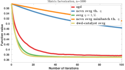
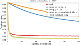
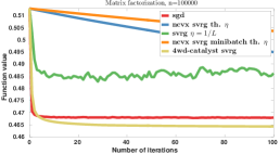
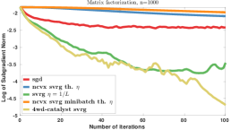
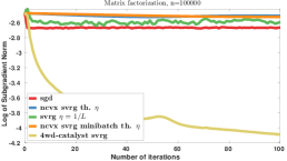
Figure 2: Dictionary learning experiments using SVRG. We plot the function value (top) and the subgradient norm (bottom). From left to right, we vary the size of dataset from $n=1\,000$  to $n=100\,000$.

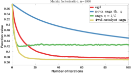
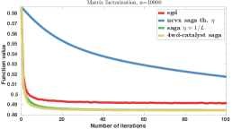
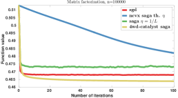
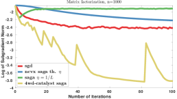
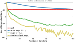
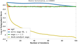
Figure 3: Dictionary learning experiments using SAGA. We plot the function value (top) and the subgradient norm (bottom). From left to right, we vary the size of dataset from $n=1\,000$  to $n=100\,000$.

Neural networks.

We consider now simple binary classification problems for learning neural networks. Assume that we are given a training set $\{a_{i},b_{i}\}_{i=1}^{n}$, where the variables $b_{i}$ in $\{-1,+1\}$ represent class labels, and $a_{i}$ in ${\mathbb{R}}^{p}$ are feature vectors. The estimator of a label class is now given by a two-layer neural network $\hat{b}=\text{sign}(w_{2}^{\top}\sigma(W_{1}^{\top}a))$, where $W_{1}$ in ${\mathbb{R}}^{p\times d}$ represents the weights of a hidden layer with $d$ neurons, $w_{2}$ in ${\mathbb{R}}^{d}$ carries the weight of the network’s second layer, and $\sigma(u)=\log(1+e^{u})$ is a non-linear function, applied pointwise to its arguments. We fix the number of hidden neurons to $d=100$ and use the logistic loss to fit the estimators to the true labels. Since the memory required by SAGA becomes $n$ times larger than SVRG for nonlinear models, which is problematic for large $n$, we can only perform experiments with SVRG. The experimental results are reported on two datasets alpha and covtype in Figures 4 and 5.

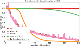
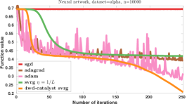
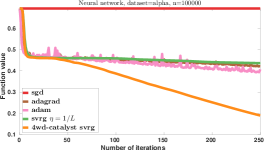
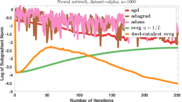
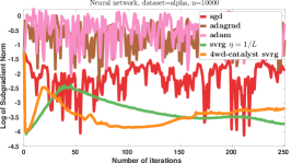
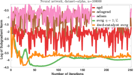
Figure 4: Neural network experiments on subsets of dataset alpha. From left to right, we vary the size of the dataset’s subset from $n=1\,000$ to $n=100\,000$.

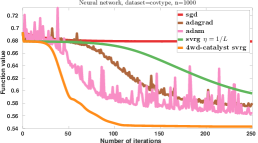
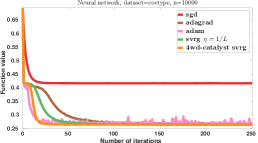
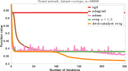
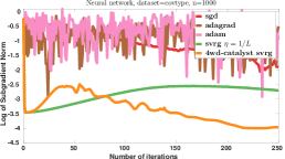
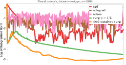
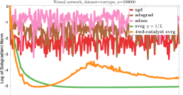
Figure 5: Neural network experiments on subsets of datasets alpha (top) and covtype (bottom).

Initial estimates of $L$.

The proposed algorithm 4WD-Catalyst requires an initial estimate of the Lipschitz constant $L$. In the problems we are considering, there is no simple closed form formula available to compute an estimate of $L$. We use the following heuristics to estimate $L$:

1. For matrix factorization, it can be shown that the function $f_{i}$ defined in (24) is differentiable according to Danskin’s theorem [see Bertsekas [6], Proposition B.25] and its gradient is given by

   $$\nabla_{D}f_{i}(D)=-(x_{i}-D\alpha_{i}(D))\alpha_{i}(D)^{T}\quad\text{ where }\quad\alpha_{i}(D)\in\operatornamewithlimits{argmin}_{\alpha\in{\mathbb{R}}^{p}}\frac{1}{2}\left\|x_{i}-D\alpha\right\|^{2}+\psi(\alpha).$$

   If the coefficients $\alpha_{i}$ were fixed, the gradient would be linear in $D$ and thus admit $\left\|\alpha_{i}\right\|^{2}$ as Lipschitz constant. Therefore, when initializing our algorithm at $D_{0}$, we find $\alpha_{i}(D_{0})$ for any $i\in[1,n]$ and use $\max_{i\in[1,n]}{\left\|\alpha_{i}(D_{0})\right\|^{2}}$ as an estimate of $L$.

2. For neural networks, the formulation we are considering is differentiable. We randomly generate two pairs of weight vectors $(W_{1},W_{2})$ and $(W_{1}^{\prime},W_{2}^{\prime})$ and use the quantity

   $$\max_{i\in[1,n]}\left\{\frac{\left\|\nabla f_{i}(W_{1},W_{2})-\nabla f_{i}(W_{1}^{\prime},W_{2})\right\|}{\left\|W_{1}-W_{1}^{\prime}\right\|},\frac{\left\|\nabla f_{i}(W_{1},W_{2})-\nabla f_{i}(W_{1},W_{2}^{\prime})\right\|}{\left\|W_{2}-W_{2}^{\prime}\right\|}\right\}$$

   as an estimate of the Lipschitz constant, where $f_{i}$ denotes the loss function respect to $i$-th training sample $(a_{i},b_{i})$. We separate weights in each layer to estimate the Lipschitz constant per layer. Indeed the scales of the weights can be quite different across layers.

Computational cost.

For SGD, AdaGrad, Adam, and all the ncvx-SVRG/SAGA variants, one iteration corresponds to one pass over the data in the plots. On the one hand, since 4WD-Catalyst-SVRG/SAGA solves two sub-problems per iteration, the cost per iteration is twice as large as the other algorithms. In our experiments, we observe that every time acceleration occurs then $\tilde{x}_{k}$ is almost always preferred to $\bar{x}_{k}$ in step 4 of 4WD-Catalyst, half of the computations are in fact not performed when running 4WD-Catalyst-SVRG/SAGA.

We report in Figure 6 an experimental study where we vary $S$ on the neural network example. In terms of number of iterations, of course, the larger $S_{k}$ the better the performance. This is not surprising as we solve each subproblem more accurately. Nevertheless, in terms of number of gradient evaluations, the relative performance is reversed. There is clearly no benefit to take larger $S_{k}$. This justifies in hindsight our choice of setting $S=n$.

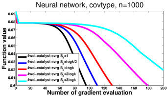
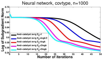
Figure 6: We run 50 iterations of 4WD-Catalyst SVRG with different choice of S on two-layer neural network. The data is a subset of dataset covtype. The x-axis is the number of gradient evaluations on the left, which is $T+S_{k}$ per iteration with $T=1$; and the number of iterations on the right.

Experimental conclusions.

In the matrix factorization experiments in Fig. 2 and Fig. 3, 4WD-Catalyst-SVRG/SAGA were always competitive, with a similar performance to the heuristic SVRG/SAGA-$\eta=1/L$ in two cases out of three, while being significantly better as soon as the amount of data $n$ was large enough. As expected, the variants of SVRG with theoretical stepsizes have slow convergence, but exhibit a stable behavior compared to SVRG-$\eta=1/L$. This confirms the remarkable ability of 4WD-Catalyst-SVRG/SAGA to adapt to nonconvex terrains.

In the neural network experiments, we observe that 4WD-Catalyst-SVRG converges much faster overall in terms of objective values than other algorithms. Yet Adam and AdaGrad often perform well-during the first iterations, they oscillate a lot, which is a behavior commonly observed. In constrast, 4WD-Catalyst-SVRG always decreases and keeps decreasing while other algorithms tend to stabilize, hence achieving significantly lower objective values.

More interestingly, as the algorithm proceeds, the subgradient norm may increase at some point and then decrease, while the function value keeps decreasing. This suggests that the extrapolation step, or the Auto-adapt procedure, is helpful to escape bad stationary points, e.g., saddle-points. We leave the study of this particular phenomenon as a potential direction for future work.

Acknowledgments.

The authors would like to thank J. Duchi for fruitful discussions related to this work. C. Paquette was partially supported by the “Learning in Machines and Brains” program of CIFAR. H. Lin and J. Mairal were supported by ERC grant SOLARIS (# 714381) and ANR grant MACARON (ANR-14-CE23-0003-01). D. Drusvyatskiy was supported by AFOSR YIP FA9550-15-1-0237, NSF DMS 1651851, and NSF CCF 1740551 awards. Z. Harchaoui was supported by NSF CCF 1740551 award, the “Learning in Machines and Brains” program of CIFAR, and faculty research awards. This work was performed while C. Paquette was at University of Washington and H. Lin was at Inria.

Appendix A Convergence rates in strongly-convex composite minimization

We now briefly discuss convergence rates, which are typically given in different forms in the convex and non-convex cases. If the weak-convex constant is known, we can form a strongly convex approximation similar to [31]. For that purpose, we consider a strongly-convex composite minimization problem

$$\min_{x\in{\mathbb{R}}^{p}}~{}h(x):=f_{0}(x)+\psi(x),$$

where $f_{0}\colon{\mathbb{R}}^{p}\to{\mathbb{R}}$ is $\mu$-strongly convex and smooth with $L$-Lipschitz continuous gradient $\nabla f_{0}$, and $\psi\colon{\mathbb{R}}^{p}\to\overline{\mathbb{R}}$ is a closed convex function with a computable proximal map

$${\rm prox}_{\beta\psi}(y):=\operatornamewithlimits{argmin}_{z\in{\mathbb{R}}^{p}}\left\{\psi(y)+\tfrac{1}{2\beta}\|z-y\|^{2}\right\}.$$

Let $x^{*}$ be the minimizer of $h$ and $h^{*}$ be the minimal value of $h$. In general, there are three types of measures of optimality that one can monitor: $\|x-x^{*}\|^{2}$, $h(x)-h^{*}$, and $\text{dist}(0,\partial h(x))$.

Since $h$ is strongly convex, the three of them are equivalent in terms of convergence rates if one can take an extra prox-gradient step:

$$[x]_{L}:={\rm prox}_{\psi/L}(x-L^{-1}\nabla f_{0}(x)).$$

To see this, define the displacement vector, also known as the gradient mapping, $g_{L}(x):=L(x-[x]_{L})$, and notice the inclusion $g_{L}(x)\in\partial h([x]_{L})$. In particular $g_{L}(x)=0$ if and only if $x$ is the minimizer of $h$. These next inequalities follow directly from Theorem 2.2.7 in [37]:

$$\tfrac{1}{2L}\|g_{L}(x)\|\leq \|x-x^{*}\|\leq\tfrac{2}{\mu}\|g_{L}(x)\|$$

$$\tfrac{\mu}{2}\|x-x^{*}\|^{2}\leq h(x)-h^{*}\leq\tfrac{1}{2\mu}|\partial h(x)|^{2}$$

$$2\mu(h([x]_{L})-h^{*})\leq \|g_{L}(x)\|^{2}\leq 2L(h(x)-h([x]_{L}))$$

Thus, an estimate of any one of the four quantities $\|x-x^{*}\|$, $h(x)-h^{*}$, $\|g_{L}(x)\|$, or $\text{dist}(0,\partial h(x))$ directly implies an estimate of the other three evaluated either at $x$ or at $[x]_{L}$.

Appendix B Theoretical analysis of the basic algorithm

We present here proofs of the theoretical results of the paper. All throughout the proofs, we shall work under the Assumptions on $f$ stated in Section 4 and the Assumptions on $\mathcal{M}$ stated in Section 5.

B.1 Convergence guarantee of Basic 4WD-Catalyst 

In Theorem 4.1 and Theorem 4.2 under an appropriate tolerance policy on the proximal subproblems (7) and (9), Basic 4WD-Catalyst performs no worse than an exact proximal point method in general, while automatically accelerating when $f$ is convex. For this, we need the following observations.

Lemma B.1 (Growth of $(\alpha_{k})$).

Suppose the sequence $\{\alpha_{k}\}_{k\geq 1}$ is produced by Algorithm 1. Then, the following bounds hold for all $k\geq 1$:

$$\frac{\sqrt{2}}{k+2}\leq\alpha_{k}\leq\frac{2}{k+1}.$$

Proof.

This result is noted without proof in a remark of [52]. For completeness, we give below a simple proof using induction. Clearly, the statement holds for $k=1$. Assume the inequality on the right-hand side holds for $k$. By using the induction hypothesis, we get

$$\alpha_{k+1}=\frac{\sqrt{\alpha_{k}^{4}+4\alpha_{k}^{2}}-\alpha_{k}^{2}}{2}=\frac{2}{\sqrt{1+4/\alpha_{k}^{2}}+1}\leq\frac{2}{\sqrt{1+(k+1)^{2}}+1}\leq\frac{2}{k+2},$$

as claimed and the expression for $\alpha_{k+1}$ is given by explicitly solving (11). To show the lower bound, we note that for all $k\geq 1$, we have

$$\alpha_{k+1}^{2}=(1-\alpha_{k+1})\alpha_{k}^{2}=\prod_{i=2}^{k+1}(1-\alpha_{i})\alpha_{1}^{2}=\prod_{i=2}^{k+1}(1-\alpha_{i}).$$

Using the established upper bound $\alpha_{k}\leq\frac{2}{k+1}$ yields

$$\alpha_{k+1}^{2}\geq\prod_{i=2}^{k+1}\left(1-\frac{2}{i+1}\right)=\frac{2}{(k+2)(k+1)}\geq\frac{2}{(k+2)^{2}}.$$

The result follows. ∎

Lemma B.2 (Prox-gradient and near-stationarity).

Suppose $y^{+}$ satisfies $\text{dist}(0,\partial f_{\kappa}(y^{+};y))<\varepsilon$. Then, the inequality holds:

$$\text{\rm dist}\big{(}0,\partial f(y^{+})\big{)}\leq\varepsilon+\left\|\kappa(y^{+}-y)\right\|.$$

Proof.

We can find $\xi\in\partial f_{\kappa}(y^{+};y)$ with $\left\|\xi\right\|\leq\varepsilon$. Taking into account $\partial f_{\kappa}(y^{+};y)=\partial f(y^{+})+\kappa(y^{+}-y)$ the result follows. ∎

Next we establish convergence guarantees of Theorem 4.1 and Theorem 4.2 for Basic 4WD-Catalyst .

Proof of Theorem 4.1 and Theorem 4.2.

The proof of Theorem 4.1 follows the analysis of inexact proximal point method [31, 22, 7]. The descent condition in (13) implies $\{f(x_{k})\}_{k\geq 0}$ are monotonically decreasing. From this, we deduce

$$f(x_{k-1})=f_{\kappa}(x_{k-1};x_{k-1})\geq f_{\kappa}(\bar{x}_{k};x_{k-1})\geq f(x_{k})+\frac{\kappa}{2}\left\|\bar{x}_{k}-x_{k-1}\right\|^{2}.$$ (25)

Using the adaptive stationarity condition (13), we apply Lemma B.2 with $y=x_{k-1}$, $y^{+}=\bar{x}_{k}$ and $\varepsilon=\kappa\left\|\bar{x}_{k}-x_{k-1}\right\|$; hence we obtain

$$\text{dist}(0,\partial f(\bar{x}_{k}))\leq 2\left\|\kappa(\bar{x}_{k}-x_{k-1})\right\|.$$

We combine the above inequality with (25) to deduce

$$\text{dist}^{2}(0,\partial f(\bar{x}_{k}))\leq 4\left\|\kappa(\bar{x}_{k}-x_{k-1})\right\|^{2}\leq 8\kappa\left(f(x_{k-1})-f(x_{k})\right).$$ (26)

Summing $j=1$ to $N$, we conclude

$$\min_{j=1,\ldots,N}~{}\big{\{}\text{dist}^{2}(0,\partial f(\bar{x}_{j}))\big{\}} \leq\frac{4}{N}\sum_{j=1}^{N}\left\|\kappa(\bar{x}_{k}-x_{k-1})\right\|^{2})$$

$$\leq\frac{8\kappa}{N}\left(\sum_{j=1}^{N}f(x_{j-1})-f(x_{j})\right)$$

$$\leq\frac{8\kappa}{N}\left(f(x_{0})-f^{*}\right).$$

Next, suppose the function $f$ is convex. Our analysis is similar to that of [52, 5]. Using the stopping criteria (14), fix an $\xi_{k}\in\partial f_{\kappa}(\tilde{x}_{k};y_{k})$ with $\left\|\xi_{k}\right\|<\frac{\kappa}{k+1}\left\|\tilde{x}_{k}-y_{k}\right\|$. For any $x\in{\mathbb{R}}^{n}$, Equation (12), and the strong convexity of the function $f_{\kappa}(\cdot;y_{k})$ yields

$$f(x_{k})\leq f(\tilde{x}_{k})\leq f(x)+\frac{\kappa}{2}\left(\left\|x-y_{k}\right\|^{2}-\left\|x-\tilde{x}_{k}\right\|^{2}-\left\|\tilde{x}_{k}-y_{k}\right\|^{2}\right)+\xi^{T}_{k}\left(\tilde{x}_{k}-x\right).$$

We substitute $x=\alpha_{k}x^{*}+(1-\alpha_{k})x_{k-1}$ where $x^{*}$ is any minimizer of $f$. Using the convexity of $f$, the norm of $\xi_{k}$, and Equations (8) and (10), we deduce

$$f(x_{k})\leq\alpha_{k}f(x^{*}) +(1-\alpha_{k})f(x_{k-1})+\frac{\alpha_{k}^{2}\kappa}{2}\left(\left\|x^{*}-v_{k-1}\right\|^{2}-\left\|x^{*}-v_{k}\right\|^{2}\right)$$

$$-\frac{\kappa}{2}\left\|\tilde{x}_{k}-y_{k}\right\|^{2}+\frac{\alpha_{k}\kappa}{k+1}\left\|\tilde{x}_{k}-y_{k}\right\|\left\|x^{*}-v_{k}\right\|.$$ (27)

Set $\theta_{k}=\frac{1}{k+1}$. Completing the square on Equation (27), we obtain

$$\frac{-\kappa}{2}\left\|\tilde{x}_{k}-y_{k}\right\|^{2}+\alpha_{k}\theta_{k}\kappa\left\|\tilde{x}_{k}-y_{k}\right\|\left\|x^{*}-v_{k}\right\|\leq\frac{\kappa}{2}\left(\alpha_{k}\theta_{k}\right)^{2}\left\|x^{*}-v_{k}\right\|^{2}.$$

Hence, we deduce

$$f(x_{k})-f^{*} \leq(1-\alpha_{k})(f(x_{k-1})-f^{*})+\frac{\alpha_{k}^{2}\kappa}{2}\left(\left\|x^{*}-v_{k-1}\right\|^{2}-\left\|x^{*}-v_{k}\right\|^{2}\right)$$

$$\qquad\qquad+\frac{\kappa}{2}\left(\alpha_{k}\theta_{k}\right)^{2}\left\|x^{*}-v_{k}\right\|^{2}.$$

$$=(1-\alpha_{k})(f(x_{k-1})-f^{*})+\frac{\alpha_{k}^{2}\kappa}{2}\left(\left\|x^{*}-v_{k-1}\right\|^{2}-\left(1-\theta_{k}^{2}\right)\left\|x^{*}-v_{k}\right\|^{2}\right)$$

Denote $A_{k}:=1-\theta_{k}^{2}$. Subtracting $f^{*}$ from both sides and using the inequality $\frac{1-\alpha_{k}}{\alpha_{k}^{2}}=\frac{1}{\alpha_{k-1}^{2}}$ and $\alpha_{1}\equiv 1$, we derive the following recursion argument:

$$\frac{f(x_{k})-f^{*}}{\alpha_{k}^{2}}+\frac{A_{k}\kappa}{2}\left\|x^{*}-v_{k}\right\|^{2} \leq\frac{1-\alpha_{k}}{\alpha_{k}^{2}}\big{(}f(x_{k-1})-f^{*}\big{)}+\frac{\kappa}{2}\left\|x^{*}-v_{k-1}\right\|^{2}$$

$$\leq\frac{1}{A_{k-1}}\left(\frac{f(x_{k-1})-f^{*}}{\alpha_{k-1}^{2}}+\frac{A_{k-1}\kappa}{2}\left\|x^{*}-v_{k-1}\right\|^{2}\right).$$

The last inequality follows because $0<A_{k-1}\leq 1$. Iterating $N$ times,we deduce

$$\frac{f(x_{N})-f^{*}}{\alpha_{N}^{2}}\leq\prod_{j=2}^{N}\frac{1}{A_{j-1}}\left(\frac{\kappa}{2}\left\|x^{*}-v_{0}\right\|^{2}\right).$$ (28)

We note

$$\prod_{j=2}^{N}\frac{1}{A_{j-1}}=\frac{1}{\prod_{j=2}^{N}\left(1-\frac{1}{(j+1)^{2}}\right)}\leq 2;$$ (29)

thereby concluding the result. Summing up (26) from $j=N+1$ to $2N$, we obtain

$$\min_{j=1,\ldots,2N}~{}\big{\{}\text{dist}^{2}(0,\partial f(\bar{x}_{j}))\big{\}} \leq\frac{4}{N}\sum_{j=N+1}^{2N}\left\|\kappa(\bar{x}_{k}-x_{k-1})\right\|^{2})$$

$$\leq\frac{8\kappa}{N}\left(\sum_{j=N+1}^{2N}f(x_{j-1})-f(x_{j})\right)$$

$$\leq\frac{8\kappa}{N}\left(f(x_{N})-f^{*}\right)$$

Combining this inequality with (28), the result is shown. ∎

Appendix C Analysis of 4WD-Catalyst and Auto-adapt

Linear convergence interlude.

Our assumption on the linear rate of convergence of $\mathcal{M}$ (see (16)) may look strange at first sight. Nevertheless, most linearly convergent first-order methods $\mathcal{M}$ for composite minimization either already satisfy this assumption or can be made to satisfy it by introducing an extra prox-gradient step. To see this, recall the convex composite minimization problem from Section A

$$\min_{z\in{\mathbb{R}}^{p}}~{}h(z):=f_{0}(z)+\psi(z),$$

where

1. $f_{0}\colon{\mathbb{R}}^{p}\to{\mathbb{R}}$ is convex and $C^{1}$-smooth with the gradient $\nabla f_{0}$ that is $L$-Lipschitz,

2. $\psi\colon{\mathbb{R}}^{p}\to\overline{\mathbb{R}}$ is a closed convex function with a computable proximal map

   $${\rm prox}_{\beta\psi}(y):=\operatornamewithlimits{argmin}_{z}~{}\{\psi(y)+\tfrac{1}{2\beta}\|z-y\|^{2}\}.$$

See [43] for a survey of proximal maps. Typical linear convergence guarantees of an optimization algorithm assert existence of constants $A\in{\mathbb{R}}$ and $\tau\in(0,1)$ satisfying

$$h(z_{t})-h^{*}\leq A(1-\tau)^{t}(h(z_{0})-h^{*})$$ (30)

for each $t=0,1,2,\ldots,\infty$. To bring such convergence guarantees into the desired form (16), define the prox-gradient step

$$[z]_{L}:={\rm prox}_{\psi/L}(z-L^{-1}\nabla f_{0}(z)),$$

and the displacement vector

$$g_{L}(z)=L(z-[z]_{L}),$$

and notice the inclusion $g_{L}(z)\in\partial h([z]_{L})$. The following inequality follows from [40]:

$$\|g_{L}(z)\|^{2}\leq 2L(h(z)-h([z]_{L}))\leq 2L(h(z)-h^{*}).$$

Thus, the linear rate of convergence (30) implies

$$\|g_{L}(z_{t})\|^{2}\leq 2LA(1-\tau)^{t}(h(z_{0})-h^{*}),$$

which is exactly in the desired form (16).

C.1 Convergence analysis of the adaptive algorithm: 4WD-Catalyst

First, under some reasonable assumptions on the method $\mathcal{M}$ (see Section 5.1), the sub-method Auto-adapt terminates.

Lemma C.1 (Auto-adapt terminates).

Assume that $\tau_{\kappa}\to 1$ when $\kappa\to+\infty$. The procedure Auto-adapt$(x,\kappa,\varepsilon,T)$ terminates after finitely many iterations.

Proof.

Due to our assumptions on $\mathcal{M}$ and the expressions $f_{\kappa}(x;x)=f(x)$ and $f_{\kappa}^{*}(x)\geq f^{*}$, we have

$$\text{\rm dist}^{2}\big{(}0,\partial f_{\kappa}(z_{T};x)\big{)}\leq A(1-\tau_{\mathcal{\kappa}})^{T}\big{(}f(x)-f_{\kappa}^{*}(x)\big{)}\leq A(1-\tau_{\kappa})^{T}\big{(}f(x)-f^{*})\big{)}.$$ (31)

Since $\tau_{\kappa}$ tends to one, for all sufficiency large $\kappa$, we can be sure that the right-hand-side is smaller than $\varepsilon^{2}$. On the other hand, for $\kappa>\rho$, the function $f_{\kappa}(\cdot;x)$ is $(\kappa-\rho)$-strongly convex and therefore we have $\text{dist}^{2}(0,\partial f_{\kappa}(z_{T};x))\geq 2(\kappa-\rho)(f_{\kappa}(z_{T};x)-f_{\kappa}^{*}(x))$. Combining this with (31), we deduce

$$f_{\kappa}(z_{T};x)-f_{\kappa}^{*}(x)\leq\frac{A(1-\tau_{\mathcal{\kappa}})^{T}}{2(\kappa-\rho)}\big{(}f(x)-f_{\kappa}^{*}(x)\big{)}.$$

Letting $\kappa\to\infty$, we deduce $f_{\kappa}(z_{T};x)\leq f(x)$, as required. Thus the loop indeed terminates. ∎

We prove the main result, Theorem 5.5, for 4WD-Catalyst.

Proof of Theorem 5.5.

The proof closely resembles the proofs of Theorem 4.2 and Theorem 4.2, so we omit some of the details. The main difference in the proof is that we keep track of the effects the parameters $\kappa_{\text{\rm cvx}}$ and $\kappa_{0}$ have on the inequalities as well as the sequence of $\kappa_{k}$. Since $\{f(x_{k})\}_{k\geq 0}$ are monotonically decreasing, we deduce

$$f(x_{k-1})=f_{\kappa_{k}}(x_{k-1};x_{k-1})\geq f_{\kappa_{k}}(\bar{x}_{k};x_{k-1})\geq f(x_{k})+\frac{\kappa_{k}}{2}\left\|\bar{x}_{k}-x_{k-1}\right\|^{2}.$$ (32)

Using the adaptive stationary condition (20), we apply Lemma B.2 with $\varepsilon=\kappa_{k}\left\|\bar{x}_{k}-x_{k-1}\right\|$; hence we obtain

$$\text{dist}(0,\partial f(\bar{x}_{k}))\leq 2\left\|\kappa_{k}(\bar{x}_{k}-x_{k-1})\right\|.$$

We combine the above inequality with (32) to deduce

$$\text{dist}^{2}(0,\partial f(\bar{x}_{k}))\leq 4\left\|\kappa_{k}(\bar{x}_{k}-x_{k-1})\right\|^{2}\leq 8\kappa_{\max}\left(f(x_{k-1})-f(x_{k})\right).$$ (33)

Summing $j=1$ to $N$, we conclude

$$\min_{j=1,\ldots,N}~{}\big{\{}\text{dist}^{2}(0,\partial f(\bar{x}_{j}))\big{\}} \leq\frac{4}{N}\sum_{j=1}^{N}2\left\|\kappa_{k}(\bar{x}_{k}-x_{k-1})\right\|^{2})$$

$$\leq\frac{8\kappa_{\max}}{N}\left(\sum_{j=1}^{N}f(x_{j-1})-f(x_{j})\right)$$

$$\leq\frac{8\kappa_{\max}}{N}\left(f(x_{0})-f^{*}\right).$$

Suppose the function $f$ is convex. Using in the stopping criteria (19) in replacement of (13), we deduce a similar expression as (27):

$$f(x_{k})\leq\alpha_{k}f(x^{*}) +(1-\alpha_{k})f(x_{k-1})+\frac{\alpha_{k}^{2}\kappa_{\text{\rm cvx}}}{2}\left(\left\|x^{*}-v_{k-1}\right\|^{2}-\left\|x^{*}-v_{k}\right\|^{2}\right)$$

$$-\frac{\kappa_{\text{\rm cvx}}}{2}\left\|\tilde{x}_{k}-y_{k}\right\|^{2}+\frac{\alpha_{k}\kappa_{\text{\rm cvx}}}{k+1}\left\|\tilde{x}_{k}-y_{k}\right\|\left\|x^{*}-v_{k}\right\|.$$

Denote $\theta_{k}=\frac{1}{k+1}$. Completing the square, we obtain

$$\frac{-\kappa_{\text{\rm cvx}}}{2}\left\|\tilde{x}_{k}-y_{k}\right\|^{2}+\alpha_{k}\theta_{k}\kappa_{\text{\rm cvx}}\left\|\tilde{x}_{k}-y_{k}\right\|\left\|x^{*}-v_{k}\right\|\leq\frac{\kappa_{\text{\rm cvx}}}{2}\left(\alpha_{k}\theta_{k}\right)^{2}\left\|x^{*}-v_{k}\right\|^{2}.$$

Hence, we deduce

$$f(x_{k})-f^{*} \leq(1-\alpha_{k})(f(x_{k-1})-f^{*})+\frac{\alpha_{k}^{2}\kappa_{\text{\rm cvx}}}{2}\left(\left\|x^{*}-v_{k-1}\right\|^{2}-\left\|x^{*}-v_{k}\right\|^{2}\right)$$

$$\qquad\qquad+\frac{\kappa_{\text{\rm cvx}}}{2}\left(\alpha_{k}\theta_{k}\right)^{2}\left\|x^{*}-v_{k}\right\|^{2}.$$

$$=(1-\alpha_{k})(f(x_{k-1})-f^{*})+\frac{\alpha_{k}^{2}\kappa_{\text{\rm cvx}}}{2}\left(\left\|x^{*}-v_{k-1}\right\|^{2}-\left(1-\theta_{k}^{2}\right)\left\|x^{*}-v_{k}\right\|^{2}\right)$$

Denote $A_{k}:=1-\theta_{k}^{2}$. Following the standard recursion argument as in the proofs of Theorem 4.2 and Theorem 4.2, we conclude

$$\frac{f(x_{k})-f^{*}}{\alpha_{k}^{2}}+\frac{A_{k}\kappa_{\text{\rm cvx}}}{2}\left\|x^{*}-v_{k}\right\|^{2} \leq\frac{1-\alpha_{k}}{\alpha_{k}^{2}}\big{(}f(x_{k-1})-f^{*}\big{)}+\frac{\kappa_{\text{\rm cvx}}}{2}\left\|x^{*}-v_{k-1}\right\|^{2}$$

$$\leq\frac{1}{A_{k-1}}\left(\frac{f(x_{k-1})-f^{*}}{\alpha_{k-1}^{2}}+\frac{A_{k-1}\kappa_{\text{\rm cvx}}}{2}\left\|x^{*}-v_{k-1}\right\|^{2}\right).$$

The last inequality follows because $0<A_{k-1}\leq 1$. Iterating $N$ times, we deduce

$$\frac{f(x_{N})-f^{*}}{\alpha_{N}^{2}}\leq\prod_{j=2}^{N}\frac{1}{A_{j-1}}\left(\frac{\kappa_{\text{\rm cvx}}}{2}\left\|x^{*}-v_{0}\right\|^{2}\right).$$ (34)

We note

$$\prod_{j=2}^{N}\frac{1}{A_{j-1}}=\frac{1}{\prod_{j=2}^{N}\left(1-\frac{1}{(j+1)^{2}}\right)}\leq 2;$$

thus the result is shown. Summing up (33) from $j=N+1$ to $2N$, we obtain

$$\min_{j=1,\ldots,2N}~{}\big{\{}\text{dist}^{2}(0,\partial f(\bar{x}_{j}))\big{\}} \leq\frac{4}{N}\sum_{j=N+1}^{2N}\left\|\kappa_{k}(\bar{x}_{k}-x_{k-1})\right\|^{2})$$

$$\leq\frac{8\kappa_{\max}}{N}\left(\sum_{j=N+1}^{2N}f(x_{j-1})-f(x_{j})\right)$$

$$\leq\frac{8\kappa_{\max}}{N}\left(f(x_{N})-f^{*}\right)$$

Combining this inequality with (34), the result is shown. ∎

Appendix D Inner-loop complexity: proof of Theorem 5.6

Recall, the following notation

$$f_{0}(x;y) =\frac{1}{n}\sum_{i=1}^{n}f_{i}(x)+\frac{\kappa}{2}\left\|x-y\right\|^{2}$$

$$y^{0} =\text{prox}_{1/(\kappa+L)f_{0}}\left(y-\frac{1}{\kappa+L}\nabla f_{0}(y;y)\right).$$ (35)

Lemma D.1 (Relationship between function values and iterates of the prox).

Assuming $\psi(x)$ is convex and the parameter $\kappa>\rho$, then

$$f_{\kappa}(y^{0};y)-f_{\kappa}^{*}(y)\leq\frac{\kappa+L}{2}\left\|y^{*}-y\right\|^{2}$$ (36)

where $y^{*}$ is a minima of $f_{\kappa}(\cdot;y)$ and $f_{\kappa}^{*}(y)$ is the optimal value.

Proof.

As the $\kappa$ is chosen sufficiently large, we know $f_{0}(\cdot;y)$ is convex and differentiable with $(\kappa+L)$-Lipschitz continuous gradient. Hence, we deduce for all $x$

$$f_{0}(y;y)+\nabla f_{0}(y;y)^{T}(x-y)\leq f_{0}(x;y).$$ (37)

Using the definition of $y^{0}$ and the $(\kappa+L)$-Lip. continuous gradient of $f_{0}(\cdot;y)$, we conclude for all $x$

$$f_{\kappa}(y^{0};y)=f_{0}(y^{0};y)+\psi(y^{0}) \leq f_{0}(y;y)+\nabla f_{0}(y;y)^{T}(y_{0}-y)+\frac{\kappa+L}{2}\left\|y_{0}-y\right\|^{2}+\psi(y_{0})$$ (38)

$$\leq f_{0}(y;y)+\nabla f_{0}(y;y)^{T}(x-y)+\frac{\kappa+L}{2}\left\|x-y\right\|^{2}+\psi(x).$$

By setting $x=y^{*}$ in both (37) and (38) and combining these results, we conclude

$$f_{\kappa}(y^{0};y)\leq f_{\kappa}^{*}(y)+\frac{\kappa+L}{2}\left\|y^{*}-y\right\|^{2}.$$

∎

Note that if we are not in the composite setting and $\kappa>\rho$, then $f_{\kappa}(\cdot,y)$ is $(\kappa+L)$-strongly convex. Using standard bounds for strongly convex functions, Equation (36) follows (see [37]). We next show an important lemma for deducing the inner complexities.

Lemma D.2.

Assume $\kappa>\rho$. Given any $\varepsilon\leq\frac{\kappa-\rho}{2}$, if an iterate $z$ satisfies $\text{dist}(0,\partial f_{\kappa}(z;y))\leq\varepsilon\left\|y^{*}-y\right\|,$ then

$$\text{dist}(0,\partial f_{\kappa}(z;y))\leq 2\varepsilon\left\|z-y\right\|.$$ (39)

Proof.

Since $\kappa>\rho$, we know $f_{\kappa}(\cdot;y)$ is $(\kappa-\rho)$-strongly convex. Therefore, by [37], we know

$$\left\|z-y^{*}\right\|\leq\frac{1}{\kappa-\rho}\text{dist}(0,\partial f_{\kappa}(z;y)).$$ (40)

By the triangle inequality and Equation (40), we deduce

$$\text{dist}(0,\partial f_{\kappa}(z;y))\leq\varepsilon\left\|y^{*}-y\right\| \leq\varepsilon\big{(}\left\|y^{*}-z\right\|+\left\|z-y\right\|\big{)}$$

$$\leq\frac{\varepsilon}{\kappa-\rho}\cdot\text{dist}(0,\partial f_{\kappa}(z;y))+\varepsilon\left\|z-y\right\|$$

$$\leq\frac{1}{2}\cdot\text{dist}(0,\partial f_{\kappa}(z;y))+\varepsilon\left\|z-y\right\|.$$

The last inequality follows because of the assumption $\varepsilon\leq\frac{\kappa-\rho}{2}$. Rearranging the terms above, we get the desired result. ∎

These two lemmas together give us Theorem 5.4.

Proof of Theorem 5.4.

First, we prove that $z_{T}$ satisfies both adaptive stationary condition and the descent condition. Recall, the point $y^{0}$ is defined to be the prox or $y$ depending on if $f_{\kappa}(\cdot;y)$ is a composite form or smooth, respectively (see statement of Theorem 5.4). By Lemma D.1 (or the remark following it), the starting $y^{0}$ satisfies

$$f_{\kappa}(y^{0};y)-f_{\kappa}^{*}(y)\leq\frac{\kappa+L}{2}\left\|y^{*}-y\right\|^{2}.$$

By the linear convergence assumption of $\mathcal{M}$ (see (16)) and the above equation, after $T:=T_{\kappa}$ iterations initializing from $y^{0}$, we have

$$\text{dist}^{2}(0,\partial f_{\kappa}(z_{T};y)) \leq A_{\kappa}(1-\tau_{\kappa})^{T}\left(f_{\kappa}(y^{0};y)-f_{\kappa}^{*}(y)\right)$$ (41)

$$\leq A_{\kappa}e^{-T\cdot\tau_{\kappa}}\left(f_{\kappa}(y^{0};y)-f_{\kappa}^{*}(y)\right)$$

$$\leq\frac{(\kappa-\rho)^{2}}{8(L+\kappa)}\cdot\frac{L+\kappa}{2}\left\|y^{*}-y\right\|^{2}$$

$$\leq\frac{(\kappa-\rho)^{2}}{16}\left\|y^{*}-y\right\|^{2}.$$

Take the square root and apply Lemma D.2 yields

$$\text{dist}(0,\partial f_{\kappa}(z_{T};y))\leq\frac{\kappa-\rho}{2}\left\|z_{T}-y\right\|\leq\kappa\left\|z_{T}-y\right\|,$$

which gives the adaptive stationary condition. Next, we show the descent condition. Let $v\in\partial f_{\kappa}(z_{T};y)$ such that $\left\|v\right\|\leq(\kappa-\rho)\left\|z_{T}-y\right\|/2$, by the $(\kappa-\rho)$-strong convexity of $f_{\kappa}(\cdot;y)$, we deduce

$$f_{\kappa}(y;y) \geq f_{\kappa}(z_{T};y)+\langle v,y-z_{T}\rangle+\frac{\kappa-\rho}{2}\left\|z_{T}-y\right\|^{2}$$

$$\geq f_{\kappa}(z_{T};y)-\left\|v\right\|\left\|y-z_{T}\right\|+\frac{\kappa-\rho}{2}\left\|z_{T}-y\right\|^{2}$$

$$\geq f_{\kappa}(z_{T};y).$$

This yields the descent condition which completes the proof for $T$. The proof for $S_{\kappa}$ is similar to $T_{\kappa}$, so we omit many of the details. In this case, we only need to show the adaptive stationary condition. For convenience, we denote $S=S_{\kappa}$. Following the same argument as in Equation (41) but with $S\log(k+1)$ number of iterations, we deduce

$$\text{dist}^{2}(0,\partial f_{\kappa}(z_{S};y))\leq\frac{(\kappa-\rho)^{2}}{16(k+1)^{2}}\left\|y^{*}-y\right\|^{2}.$$

By applying Lemma D.2, we obtain

$$\text{dist}(0,\partial f_{\kappa}(z_{S};y))\leq\frac{(\kappa-\rho)}{2(k+1)}\left\|z_{T}-y\right\|\leq\frac{\kappa}{k+1}\left\|z_{S}-y\right\|,$$

which proves the desired result for $z_{S}$. ∎

Assuming Proposition 5.7 and Proposition 5.8 hold as well as Lemma D.3, we begin by providing the proof of Theorem 5.6.

Proof of Theorem 5.6.

We consider two cases: (i) the function $f$ is non-convex and (ii) the function $f$ is convex. First, we consider the non-convex setting. To produce $\bar{x}_{k}$, the method $\mathcal{M}$ is called

$$T\log\left(\tfrac{4L}{\kappa_{0}}\right)/\log(2)$$ (42)

number of times. This follows from Proposition 5.7 and Lemma D.3. The reasoning is that once $\kappa>\rho+L$, which only takes at most $\log(4L/\kappa_{0})$ number of increases of $\kappa$ to reach, then the iterate $\bar{x}_{k}$ satisfies the stopping criteria (20). Each time we increase $\kappa$ we run $\mathcal{M}$ for $T$ iterations. Therefore, the total number of iterations of $\mathcal{M}$ is given by multiplying $T$ with $\log(4L/\kappa_{0})$. To produce $\tilde{x}_{k}$, the method $\mathcal{M}$ is called $S\log(k+1)$ number of times. (Note: the proof of Theorem 5.5 does not need $\tilde{x}_{k}$ to satisfy (19) in the non-convex case).

Next, suppose the function $f$ is convex. As before, to produce $\bar{x}_{k}$ the method $\mathcal{M}$ is called (42) times. To produce $\tilde{x}_{k}$, the method $\mathcal{M}$ is called $S\log(k+1)$ number of times. By Proposition 5.8, the iterate $\tilde{x}_{k}$ satisfies (19); a key ingredient in the proof of Theorem 5.5. ∎

D.1 Inner complexity for $\bar{x}_{k}$: proof of Proposition 5.7

Next, we supply the proof of Proposition 5.7 which shows that by choosing $\kappa$ large enough, Algorithm 3 terminates.

Proof of Proposition 5.7.

The idea is to apply Theorem 5.4. Since the parameter $A_{\kappa}$ increases with $\kappa$, then we upper bound it by $A_{\kappa_{k}}\leq A_{4L}$. Moreover, we have $\kappa-\rho\geq\rho+L-\rho=L$. Lastly, since $\tau_{\kappa}$ is increasing in $\kappa$, we know $\frac{1}{\tau_{\kappa}}\leq\frac{1}{\tau_{L}}$. Plugging these bound into Theorem 5.4, we see that for any smoothing parameter $\kappa$ satisfying $\rho+L<\kappa<4L$, we get the desired result. ∎

Next, we compute the maximum number of times we must double $\kappa$ until $\kappa>\rho+L$.

Lemma D.3 (Doubling $\kappa$).

If we set $T$ and $S$ according to Theorem 5.6, then the doubling of $\kappa_{0}$ will terminate as soon as $\kappa>\rho+L$. Thus the number of times $\kappa_{0}$ must be doubled in Algorithm 3 is at most

$$\frac{\log\left(\frac{2(\rho+L)}{\kappa_{0}}\right)}{\log(2)}\leq\left\lceil\frac{\log\left(\frac{4L}{\kappa_{0}}\right)}{\log(2)}\right\rceil.$$

Since $\kappa$ is doubled (Algorithm 3) and $T$ is chosen as in Proposition 5.7 , the maximum the value $\kappa$, $\kappa_{\max}$, takes is $2(\rho+L)\leq 4L$.

D.2 Inner complexity for $\tilde{x}_{k}$: proof of Proposition 5.8

In this section, we prove Proposition 5.8, an inner complexity result for the iterates $\tilde{x}_{k}$. Recall that the inner-complexity analysis for $\tilde{x}_{k}$ is important only when $f$ is convex (see Section 5). Therefore, we assume throughout this section that the function $f$ is convex. We are now ready to prove Proposition 5.8.

Proof of Proposition 5.8.

The proof immediately follows from Theorem 5.4 by setting $\kappa=\kappa_{\text{cvx}}$ and $\rho=0$ as the function $f$ is convex. ∎

Proof of Theorem 5.3.

Since $\rho$ is known, we let $\kappa=2\rho$ for $S$ and $\kappa=\kappa_{\text{\rm cvx}}$ for $T$ in Theorem 5.4. Therefore, the number of iterations is to produce $\bar{x}_{k}$ is $S_{2\rho}\leq S_{2L}$ and $\tilde{x}_{k}$ is $T_{\kappa_{\text{\rm cvx}}}$. Combining this with Theorem 4.2 for the outer complexity, the result is shown. ∎

References

- [1] Z. Allen-Zhu. Katyusha: The first direct acceleration of stochastic gradient methods. In Symposium on Theory of Computing (STOC), 2017.
- [2] Z. Allen-Zhu. Natasha: Faster non-convex stochastic optimization via strongly non-convex parameter. In International conference on machine learning (ICML), 2017.
- [3] Z. Allen-Zhu and E. Hazan. Variance reduction for faster non-convex optimization. In International conference on machine learning (ICML), 2016.
- [4] Z. Allen-Zhu and Y. Yuan. Improved SVRG for Non-Strongly-Convex or Sum-of-Non-Convex Objectives. In International conference on machine learning (ICML), 2016.
- [5] A. Beck and M. Teboulle. A fast iterative shrinkage-thresholding algorithm for linear inverse problems. SIAM Journal on Imaging Sciences, 2(1):183–202, 2009.
- [6] D. P. Bertsekas. Nonlinear programming. Athena scientific Belmont, 1999.
- [7] D. P. Bertsekas. Convex Optimization Algorithms. Athena Scientific, 2015.
- [8] J. Bolte, T. P. Nguyen, J. Peypouquet, and B. Suter. From error bounds to the complexity of first-order descent methods for convex functions. Mathematical Programming, Series A, 165:471–507, 2016.
- [9] J. M. Borwein and A. S. Lewis. Convex analysis and nonlinear optimization: theory and examples. Springer Verlag, 2006.
- [10] Y. Carmon, J. C. Duchi, O. Hinder, and A. Sidford. Lower bounds for finding stationary points I. preprint arXiv:1710.11606, 2017.
- [11] Y. Carmon, J. C. Duchi, O. Hinder, and A. Sidford. Accelerated methods for non-convex optimization. SIAM Journal on Optimization, 28(2):1751–1772, 2018.
- [12] Y. Carmon, O. Hinder, J. C. Duchi, and A. Sidford. “convex until proven guilty”: Dimension-free acceleration of gradient descent on non-convex functions. In International conference on machine learning (ICML), 2017.
- [13] C. Cartis, N. I. M. Gould, and P. L. Toint. On the complexity of steepest descent, newton’s and regularized newton’s methods for nonconvex unconstrained optimization problems. SIAM Journal on Optimization, 20(6):2833–2852, 2010.
- [14] C. Cartis, N.I.M. Gould, and P. L. Toint. On the complexity of finding first-order critical points in constrained nonlinear optimization. Mathematical Programming, Series A, 144:93–106, 2014.
- [15] F. H. Clarke, R. J. Stern, and P. R. Wolenski. Proximal smoothness and the lower- property. Journal of Convex Analysis, 2(1-2):117–144, 1995.
- [16] A. J. Defazio, F. Bach, and S. Lacoste-Julien. SAGA: A fast incremental gradient method with support for non-strongly convex composite objectives. In Advances in Neural Information Processing Systems (NIPS), 2014.
- [17] D. Drusvyatskiy and C. Paquette. Efficiency of minimizing compositions of convex functions and smooth maps. Mathematical Programming, (Ser. A):1–56, 2018.
- [18] J. C. Duchi, E. Hazan, and Y. Singer. Adaptive subgradient methods for online learning and stochastic optimization. Journal of Machine Learning Research (JMLR), 12:2121–2159, 2011.
- [19] H. Federer. Curvature measures. Transactions of the American Mathematical Society, 93:418–491, 1959.
- [20] S. Ghadimi and G. Lan. Accelerated gradient methods for nonconvex nonlinear and stochastic programming. Mathematical Programming, 156(1-2, Ser. A):59–99, 2016.
- [21] S. Ghadimi, G. Lan, and H. Zhang. Generalized uniformly optimal methods for nonlinear programming. preprint arXiv:1508.07384, 2015.
- [22] O. Güler. On the convergence of the proximal point algorithm for convex minimization. SIAM Journal on Control and Optimization, 29(2):403–419, 1991.
- [23] T. Hastie, R. Tibshirani, and M. Wainwright. Statistical learning with sparsity: the Lasso and generalizations. CRC Press, 2015.
- [24] C. Jin, P. Netrapalli, and M. I. Jordan. Accelerated gradient descent escapes saddle points faster than gradient descent. In Conference On Learning Theory (COLT), 2018.
- [25] R. Johnson and T. Zhang. Accelerating stochastic gradient descent using predictive variance reduction. In Advances in Neural Information Processing Systems (NIPS), 2013.
- [26] Diederik P Kingma and Jimmy Ba. Adam: A method for stochastic optimization. International Conference on Learning Representations (ICLR), 2015.
- [27] G. Lan and Y. Zhou. An optimal randomized incremental gradient method. Mathematical Programming, Series A, pages 1–38, 2017.
- [28] L. Lei and M. I. Jordan. Less than a single pass: stochastically controlled stochastic gradient method. In Conference on Artificial Intelligence and Statistics (AISTATS), 2017.
- [29] L. Lei, C. Ju, J. Chen, and M. I. Jordan. Non-convex finite-sum optimization via SCSG methods. In Advances in Neural Information Processing Systems (NIPS), 2017.
- [30] H. Li and Z. Lin. Accelerated proximal gradient methods for nonconvex programming. In Advances in Neural Information Processing Systems (NIPS). 2015.
- [31] H. Lin, J. Mairal, and Z. Harchaoui. A universal catalyst for first-order optimization. In Advances in Neural Information Processing Systems (NIPS), 2015.
- [32] H. Lin, J. Mairal, and Z. Harchaoui. Catalyst Acceleration for First-order Convex Optimization: from Theory to Practice. Journal of Machine Learning Research (JMLR), 18:1–54, 2018.
- [33] J. Mairal. Incremental majorization-minimization optimization with application to large-scale machine learning. SIAM Journal on Optimization, 25(2):829–855, 2015.
- [34] J. Mairal, F. Bach, and J. Ponce. Sparse modeling for image and vision processing. Foundations and Trends in Computer Graphics and Vision, 8(2-3):85–283, 2014.
- [35] J. Mairal, F. Bach, J. Ponce, and G. Sapiro. Online learning for matrix factorization and sparse coding. Journal of Machine Learning Research (JMLR), 11:19–60, 2010.
- [36] Y. Nesterov. A method of solving a convex programming problem with convergence rate (1/). Soviet Mathematics Doklady, 27(2):372–376, 1983.
- [37] Y. Nesterov. Introductory lectures on convex optimization: a basic course. Springer, 2004.
- [38] Y. Nesterov. Efficiency of coordinate descent methods on huge-scale optimization problems. SIAM Journal on Optimization, 22(2):341–362, 2012.
- [39] Y. Nesterov. How to make the gradients small. OPTIMA, MPS Newsletter, (88):10–11, 2012.
- [40] Y. Nesterov. Gradient methods for minimizing composite functions. Mathematical Programming, 140(1):125–161, 2013.
- [41] J. Nutini, M. Schmidt, I. H. Laradji, M. P. Friedlander, and H. A. Koepke. Coordinate descent converges faster with the gauss-southwell rule than random selection. In Proc. International Conference on Machine Learning (ICML), 2015.
- [42] M. O’Neill and S. J. Wright. Behavior of accelerated gradient methods near critical points of nonconvex problems. Mathematical Programming, (Ser. B):1–25, 2018.
- [43] N. Parikh and S.P. Boyd. Proximal algorithms. Foundations and Trends in Optimization, 1(3):123–231, 2014.
- [44] R. A. Poliquin and R. T. Rockafellar. Prox-regular functions in variational analysis. Transactions of the American Mathematical Society, 348(5):1805–1838, 1996.
- [45] S. J. Reddi, A. Hefny, S. Sra, B. Poczos, and A. Smola. Stochastic variance reduction for nonconvex optimization. In International conference on machine learning (ICML), 2016.
- [46] S. J. Reddi, S. Sra, B. Poczos, and A. J. Smola. Proximal stochastic methods for nonsmooth nonconvex finite-sum optimization. In Advances in Neural Information Processing Systems (NIPS), 2016.
- [47] P. Richtarik and M. Takac. Iteration complexity of randomized block-coordinate descent methods for minimizing a composite function. Mathematical Programming, 144(1-2):1–38, 2014.
- [48] R. T. Rockafellar. Favorable classes of Lipschitz-continuous functions in subgradient optimization. In Progress in nondifferentiable optimization, volume 8 of IIASA Collaborative Proc. Ser. CP-82, pages 125–143. Internat. Inst. Appl. Systems Anal., Laxenburg, 1982.
- [49] R. T. Rockafellar and R. J.-B. Wets. Variational analysis, volume 317 of Grundlehren der Mathematischen Wissenschaften [Fundamental Principles of Mathematical Sciences]. Springer-Verlag, Berlin, 1998.
- [50] M. Schmidt, N. Le Roux, and F. Bach. Minimizing finite sums with the stochastic average gradient. Mathematical Programming, 162(1):83–112, 2017.
- [51] S. Shalev-Shwartz. SDCA without Duality, Regularization, and Individual Convexity. In International conference on machine learning (ICML), 2016.
- [52] P. Tseng. On accelerated proximal gradient methods for convex-concave optimization. Technical report, 2008.
- [53] B. E. Woodworth and N. Srebro. Tight complexity bounds for optimizing composite objectives. In Advances in Neural Information Processing Systems (NIPS). 2016.
- [54] S. J. Wright. Coordinate descent algorithms. Mathematical Programming, 151(1):3–34, June 2015.
- [55] L. Xiao and T. Zhang. A proximal stochastic gradient method with progressive variance reduction. SIAM Journal on Optimization, 24(4):2057–2075, 2014.
- [56] H. Zou and T. Hastie. Regularization and variable selection via the elastic net. Journal of the Royal Statistical Society: Series B (Statistical Methodology), 67(2):301–320, 2005.