Modified Interior-Point Method for Large-and-Sparse Low-Rank Semidefinite Programs

Abstract

Semidefinite programs (SDPs) are powerful theoretical tools that have been studied for over two decades, but their practical use remains limited due to computational difficulties in solving large-scale, realistic-sized problems. In this paper, we describe a modified interior-point method for the efficient solution of large-and-sparse low-rank SDPs, which finds applications in graph theory, approximation theory, control theory, sum-of-squares, etc. Given that the problem data is large-and-sparse, conjugate gradients (CG) can be used to avoid forming, storing, and factoring the large and fully-dense interior-point Hessian matrix, but the resulting convergence rate is usually slow due to ill-conditioning. Our central insight is that, for a rank-$k$, size-$n$ SDP, the Hessian matrix is ill-conditioned only due to a rank-$nk$ perturbation, which can be explicitly computed using a size-$n$ eigendecomposition. We construct a preconditioner to “correct” the low-rank perturbation, thereby allowing preconditioned CG to solve the Hessian equation in a few tens of iterations. This modification is incorporated within SeDuMi, and used to reduce the solution time and memory requirements of large-scale matrix-completion problems by several orders of magnitude.

I Introduction

Consider the size-$n$ semidefinite program with $m$ constraints

$$X^{\star}=\text{ minimize } C\bullet X$$ (SDP)

subject to $$A_{i}\bullet X=b_{i}\quad\forall i\in\{1,\ldots,m\}$$

$$X\succeq 0,$$

and its Lagrangian dual

$$\{y^{\star},S^{\star}\}=\text{ maximize } b^{T}y$$ (SDD)

subject to $$\sum_{i=1}^{m}y_{i}A_{i}+S=C$$

$$S\succeq 0.$$

Each matrix is $n\times n$ real symmetric (an element of $\mathbb{S}^{n}$); $\bullet$ denotes the associated matrix inner product $A\bullet B=\mathrm{tr}\,A^{T}B$; and $X\succeq 0$ and $S\succ 0$ ($X\in\mathbb{S}_{+}^{n}$ and $S\in\mathbb{S}_{++}^{n}$) indicate that $X$ is symmetric positive semidefinite and $S$ is symmetric positive definite. In case of nonunique solutions, we use $\{X^{\star},y^{\star},S^{\star}\}$ to refer to the analytic center of the solution set.

In this paper, we consider large-and-sparse low-rank SDPs, for which the number of nonzeros in the data $A_{1},\ldots,A_{m}$ is small, and $k\triangleq\mathrm{rank}\,X^{\star}$ is known a priori to be very small relative to the dimensions of the problem, i.e. $k\ll n$. Such problems widely appear as the convex relaxations of “hard” optimization problems in graph theory [1], approximation theory [2, 3, 4], control theory [5, 4, 6], and power systems [7, 8]. They are also the fundamental building blocks for global optimization techniques based upon polynomial sum-of-squares [9] and the generalized problem of moments [4].

Interior-point methods are the most reliable approach for solving small- and medium-scale SDPs, but become prohibitively time- and memory-intensive for large-scale problems. A fundamental issue is their inability to exploit problem structure, such as the sparsity of the data and the low-rank feature of the solution, to substantially reduce complexity. In other words, interior-point methods solve highly sparse, rank-one SDPs in approximately the same time as dense, full-rank SDPs of the same size.

In this paper, we present a modification to the standard interior-point method that makes it substantially more efficient for large-and-sparse low-rank SDPs. More specifically, our algorithm solves a rank-$k$ SDP in $\Theta(n^{3}k^{3})$ time and $\Theta(n^{2}k^{2})$ memory, under some mild nondegeneracy and sparsity assumptions. In Section V, we give numerical results to show that our method is up to a factor of $n$ faster than the standard interior-point method for problems with $m\sim n$ constraints, and up to a factor of $n^{3}$ faster for problems with $m\sim n^{2}$ constraints.

I-A Assumptions

We begin with some nondegeneracy assumptions, which are standard for interior-point methods.

Assumption 1 (Nondegeneracy).

We assume:

1. (Slater’s condition) There exist $X\succ 0$, $y$, and $S\succ 0$, such that $A_{i}\bullet X=b_{i}$ and $\sum_{i}y_{i}A_{i}+S=C$.

2. (Strict complementarity) $\mathrm{rank}\,(X^{\star})+\mathrm{rank}\,(S^{\star})=n$.

These are generic properties of SDPs, and are satisfied by almost all instances [10]. Note that Slater’s condition is satisfied in solvers like SeDuMi [11] and MOSEK [12] using the homogenous self-dual embedding technique [13].

We further assume that the data matrices $A_{1},\ldots,A_{m}$ are structured in a way that allow certain matrix-implicit operations to be efficiently performed.

Assumption 2 (Sparsity).

Define the matrix $\mathbf{A}\triangleq[\mathrm{vec}\,A_{1},\ldots,\mathrm{vec}\,A_{m}]$. We assume that matrix-vector products with $\mathbf{A}$, $\mathbf{A}^{T}$ and $(\mathbf{A}^{T}\mathbf{A})^{-1}$ may each be applied in $O(m)$ flops and memory.

Versions of this assumption appear in most large-scale SDP algorithms, spanning both first-order [14, 7, 15, 16, 17, 6] and second-order methods [18, 19]. The assumption is satisfied by any sparse data whose normal matrix $\mathbf{A}^{T}\mathbf{A}$ admits a sparse Cholesky factorization.

I-B Related work

The desire to effectively exploit problem structure in large-scale SDPs has motivated a number of algorithms. It is convenient to categorize them into three distinct groups:

The first group is based on using sparsity in the data to decompose the size-$n$ conic constraint $X\succeq 0$ into many smaller conic constraints over submatrices of $X$. In particular, when the matrices $C,A_{1},\ldots,A_{m}$ share a common sparsity structure with a chordal graph with bounded treewidth $\tau$, a technique known as chordal decomposition or chordal conversion can be used to reformulate (SDP)-(SDD) into a problem containing only size-$(\tau+1)$ semidefinite constraints [20]; see also [21]. While the technique is only applicable to chordal SDPs with bounded treewidths, it is able to reduce the cost of a size-$n$ SDP all the way down to the cost of a size-$n$ linear program, sometimes as low as $O(\tau^{3}n)$. Indeed, chordal sparsity can be guaranteed in many important applications [21, 8], and software exist to automate the chordal reformulation [22].

The second group is based on applying first-order methods for nonlinear programming, such as conjugate gradients [18, 19, 6] and ADMM [14, 7, 15, 16, 17], either to (SDP) directly, or to the Newton subproblem associated with an interior-point solution of (SDP). These algorithms have inexpensive per-iteration costs but a sublinear worst-case convergence rate, computing an $\epsilon$-accurate solution in $O(1/\epsilon)$ time. They are most commonly used to solve very large-scale SDPs to modest accuracy.

The third group is based on the outer product factorization $X=RR^{T}$. These methods use the low-rank of $X^{\star}$ to reduce the number of decision variables in (SDP) from $\sim n^{2}$ to $nk$ [23, 24]. The problem being solved is no longer convex, so only local convergence can be guaranteed. Nevertheless, time and memory requirements are substantially reduced, and these methods have been used to solve very large-scale low-rank SDPs to excellent precision; see the computation results in [23, 24].

Our method is similar in spirit to methods from the second group, but makes much stronger convergence guarantees. More specifically, we guarantee that the method converges globally to $\{X^{\star},y^{\star},S^{\star}\}$ at a linear rate, producing an $\epsilon$-accurate solution in $O(\log(1/\epsilon))$ time. At the same time, the method remains applicable for SDPs that are sparse but nonchordal. Indeed, in Section V, we present strong computational results for the matrix completion problem, which cannot be efficiently solved using methods from the first group. We mention, however, that the method has a higher memory requirement than methods from the third group, due to its need to explicitly store the matrix variables $X$ and $S$.

I-C Notations

Most of our notations are standard except the following. Given a positive definite matrix $X\in\mathbb{S}_{++}^{n}$, we order its eigenvalues $\lambda_{1}(X)\geq\cdots\geq\lambda_{n}(X)$, and define its condition number $\kappa(X)=\lambda_{1}(X)/\lambda_{n}(X)$. We sometimes use $\lambda_{\max}(X)\equiv\lambda_{1}(X)$ and $\lambda_{\min}(X)\equiv\lambda_{n}(X)$ for emphasis. We use “$\mathrm{vec}\,$” and “$\otimes$” to refer to the (nonsymmetricized) vectorization and Kronecker product, which satisfy the identity $\mathrm{vec}\,AXB^{T}=(A\otimes B)\mathrm{vec}\,X$. We use $\mathrm{diag}\,(A,B)=\left[\begin{smallmatrix}A&0\\ 0&B\end{smallmatrix}\right]$ to refer to the matrix direct sum.

II Interior-Point Methods

Consider replacing the nonsmooth, convex constraint $X\succeq 0$ in (SDP) by the smooth, strongly convex, and self-concordant penalty function $\mu\log\det X$, as in

$$X_{\mu}=\text{ minimize } C\bullet X-\mu\log\det X \mu$$ (SDP)

subject to $$A_{i}\bullet X=b_{i}\;\forall i\in\{1,\ldots,m\}.$$

The resulting problem has Lagrangian dual

$$\{y_{\mu},S_{\mu}\}=\text{ maximize } b^{T}y+\mu\log\det S \mu$$ (SDD)

subject to $$\sum_{i=1}^{m}y_{i}A_{i}+S=C.$$

For different values of $\mu>0$, the corresponding solutions $\{X_{\mu},y_{\mu},S_{\mu}\}$ define a trajectory in the feasible region of (SDP)-(SDD) that approaches $\{X^{\star},y^{\star},S^{\star}\}$ as $\mu\to 0^{+}$. This trajectory is known as the central path, and $\mu$ is known as the duality gap parameter, because $n\mu=X_{\mu}\bullet S_{\mu}=C\bullet X_{\mu}-b^{T}y_{\mu}$ is the duality gap of the feasible point $\{X_{\mu},y_{\mu},S_{\mu}\}$ in (SDP)-(SDD).

All interior-point methods work by using Newton’s method to approximately solve (SDP$\mu$), (SDD$\mu$), or their joint Karush–Kuhn–Tucker (KKT) equations, while making decrements in the duality gap parameter $\mu$. Most modern SDP solvers are of the path-following type, and explicitly keep their iterates within a feasible neighborhood of the central path

$$\mathcal{N}_{\infty}^{-}(\gamma) \triangleq\left\{\{X,y,S\}\text{ feas.}:\lambda_{\min}(XS)\geq\frac{\gamma}{n}\mathrm{tr}\,XS\right\},$$ (1)

where $\gamma\in(0,1)$ quantifies the “size” of the neighborhood. The resulting interior-point method has a formal iteration complexity of $O(n\log\epsilon^{-1})$, but always converges within tens of iterations in practice [25, Ch.5].

Each iteration of an interior-point method solves 1-3 quadratic approximations of (SDD$\mu$)

maximize $$b^{T}y-\frac{1}{2}\|W^{\frac{1}{2}}(S-Z)W^{\frac{1}{2}}\|_{F}^{2}$$ (2)

subject to $$\sum_{i=1}^{m}y_{i}A_{i}+S=C,$$

in which $W,Z\in\mathbb{S}_{++}^{n}$ are used by the algorithm to approximate the log-det penalty. Substituting $S=C-\sum_{i=1}^{m}y_{i}A_{i}$ into the objective (2) yields an unconstrained problem with first-order optimality conditions:

$$A_{i}\bullet\left[W\left(\sum_{j=1}^{m}y_{j}A_{j}\right)W\right]=\underbrace{b_{i}+A_{i}\bullet W(C-Z)W}_{r_{i}}$$ (3)

for all $i\in\{1,\ldots,m\}$. Vectorizing the matrix variables allows (3) to be compactly written as

$$\underbrace{(\mathbf{A}^{T}\mathbf{D}\mathbf{A})}_{\mathbf{H}}y=r$$ (4)

where $\mathbf{A}=[\mathrm{vec}\,A_{1},\ldots,\mathrm{vec}\,A_{m}]$ and $\mathbf{D}=W\otimes W$. Once $y$ is computed, the variables $S=C-\sum_{i=1}^{m}y_{i}A_{i}$ and $X=W(Z-S)W$ are easily recovered.

Since the interior-point method converges in tens of iterations, the cost of solving (SDP)-(SDD) is essentially the same as that of solving the Hessian equation $\mathbf{H}y=r$, up to a modest multiplicative constant. Or put in another way, an interior-point method can be thought of as a technique to convert the nonsmooth conic problems (SDP)-(SDD) into a small sequence of unconstrained least-squares problems [26, Ch.11].

II-A Solving the Hessian equation

The computation bottleneck in every interior-point method is the solution of the Hessian equation $\mathbf{H}y=r$. The standard approach found in the vast majority of interior-point solvers is to form $\mathbf{H}$ explicitly and to factor it using Cholesky factorization. An important feature of interior-point methods for SDPs is that the matrix $W$ is fully-dense, so the cost of forming and factoring the fully-dense $m\times m$ Hessian matrix $\mathbf{H}$ using dense Cholesky factorization is $O(n^{3}m+n^{2}m^{2}+m^{3})$ time and $\Theta(m^{2}+n^{2})$ memory.

Alternatively, the Hessian equation may be solved using an iterative method like conjugate gradients (CG). We defer to standard texts [27] for implementation details, and only note that the method requires a single matrix-vector product with the governing coefficient matrix at each iteration. In exact arithmetic, CG converges to the exact solution of the Hessian equation $\mathbf{H}y=r$ within $m$ iterations, thereby producing a complexity of $O(n^{3}m+n^{2}m^{2})$ time and $\Theta(n^{2}+m)$ memory, which is strictly better than Cholesky factorization.

However, in finite precision, CG does not terminate in $m$ steps due to the accumulation of round-off error. Instead, the method converges linearly, with a convergence rate related to the condition number of the governing matrix.

Proposition 1 ([28, p.53]).

Given $x^{0},b\in\mathbb{R}^{n}$, $A\in\mathbb{S}_{++}^{n}$, define $x^{\star}=A^{-1}b$. Then, the $i$-th iterate of CG generates satisfies

$$\frac{\|x^{i}-x^{\star}\|}{\|x^{0}-x^{\star}\|}\leq 2\sqrt{\kappa_{1}}\left(\frac{\sqrt{\kappa_{j}}-1}{\sqrt{\kappa_{j}}+1}\right)^{i-j}$$ (5)

with condition numbers $\kappa_{j}=\lambda_{j}(A)/\lambda_{\min}(A)$ and $j\in\{1,\ldots,n\}$.

The Hessian matrix $\mathbf{H}$ becomes increasing ill-conditioned as the outer interior-point method makes progress towards the solution. Its condition number scales $\kappa(\mathbf{H})=O(1/\mu^{2})$, where $\mu$ is the duality gap parameter at the current interior-point iteration. This ill-conditioning gives any CG-based interior-point method a sublinear worse-case time complexity, converging to an $\epsilon$-accurate solution of (SDP)-(SDD) in $O(1/\epsilon)$ time.

Instead, all successful CG-based solution of the Hessian equation rely on an effective preconditioner, and a modification to CG named preconditioned conjugate gradients (PCG). Each PCG iteration requires a single matrix-vector product with the governing matrix, and a single solve with the preconditioner; see e.g. [27, 28].

Proposition 2.

Given $x^{0},b\in\mathbb{R}^{n}$ , $A\in\mathbb{S}_{++}^{n}$, and preconditioner $P\in\mathbb{S}_{++}^{n}$, define $x^{\star}=A^{-1}b$. Then, the $i$-th iterate of PCG generates satisfies (5) with $\kappa_{j}=\lambda_{j}(P^{-1}A)/\lambda_{n}(P^{-1}A)$.

If a preconditioner $\tilde{\mathbf{H}}$ can be constructed to be spectrally similar to $\mathbf{H}$ (in the specific sense described in Proposition 2), then PCG allows us to solve a Hessian $\mathbf{H}y=r$ by solving a few instances of the preconditioner equation $\tilde{\mathbf{H}}y=r$.

II-B Ill-conditioning in the scaling matrix

The matrix $W\in\mathbb{S}_{++}^{n}$ is known as the scaling matrix, and captures the curvature of the log-det penalty function. Different interior-point methods differ primarily how the scaling matrix $W$ is constructed. Given the current iterate $\{\hat{X},\hat{y},\hat{S}\}$, we consider three types of scalings:

• Primal scaling. Set $W\leftarrow\hat{X}$. Used in the original projective conic interior-point method by Nesterov & Nemirovski [29].

• Dual scaling. Set $W\leftarrow\hat{S}^{-1}$. Used in the log-determinant barrier method [30].

• Nesterov-Todd (NT) scaling. Set $W$ to be the unique positive definite matrix satisfying $\hat{X}=W\hat{S}W$. This is the most widely used scaling method for semidefinite programming, found in SeDuMi [11] and MOSEK [12].

In all three cases, the scaling matrix $W$ becomes progressively ill-conditioned as the interior-point method makes progress towards the solution. This is the mechanism that causes the Hessian matrix $\mathbf{H}$ to become ill-conditioned; see [10].

Lemma 3.

Under Assumption 1, fix $\mu_{0}>0$ and $\gamma\in(0,1)$. Then, for all points $\{X,y,S\}$ with

$$\{X,y,S\}\in\mathcal{N}_{\infty}^{-}(\gamma),\qquad\mu\leq\mu_{0}$$

(where $\mu=\frac{1}{n}\mathrm{tr}\,XS$), there are constants $C_{0}$ and $C_{1}$ such that

$$\lambda_{1}(X)\leq C_{0},\qquad\lambda_{1}(S)\leq C_{0},$$ (6)

$$\lambda_{k}(X)\geq C_{1}\gamma,\qquad\lambda_{n-k}(S)\geq C_{1}\gamma,$$ (7)

$$\lambda_{k+1}(X)\leq\mu/C_{1},\qquad\lambda_{n-k+1}(S)\leq\mu/C_{1},$$ (8)

$$\lambda_{n}(X)\geq\gamma\mu/C_{0},\qquad\lambda_{n}(S)\geq\gamma\mu/C_{0}.$$ (9)

Proof:

This is the SDP version of Lemma 5.13 in [25], which was stated for LPs. ∎

Proposition 4.

Under the conditions in Lemma 3, let $W$ be the primal, dual, or NT scaling matrix computed from $\{X,S\}$. Then,

$$\frac{\lambda_{1}(W)}{\lambda_{k}(W)}=O(1),\;\frac{\lambda_{k+1}(W)}{\lambda_{n}(W)}=O(1),\;\frac{\lambda_{k}(W)}{\lambda_{k+1}(W)}=\Theta(1/\mu).$$

Proof:

Lemma 3 establishes these conditions for $X$ and $S^{-1}$. For NT scaling, let us note that $W=X\#S^{-1}$, where $\#$ is the (metric) geometric mean operator of Ando [31]. Then, Ando’s matrix arithmetic-geometric inequality implies $\frac{1}{2}(X+\mu S^{-1})\succeq X\#(\mu S^{-1})=\frac{1}{\sqrt{\mu}}W$ and $\frac{1}{2}(\mu X^{-1}+S)\succeq(\mu X^{-1})\#S=\sqrt{\mu}W^{-1}$. ∎

III Preconditioning the Hessian Matrix

In this section, we develop a preconditioner $\tilde{\mathbf{H}}$ that is both easy to invert, and also serves as a good spectral approximation for $\mathbf{H}$. More specifically, we prove that PCG with $\tilde{\mathbf{H}}$ as preconditioner solves the Hessian equation $\mathbf{H}y=r$ to machine precision in a constant number of iterations, irrespective of $\mu$.

III-A The main idea

The preconditioner is based off the observation that the scaling matrix $W$ becomes ill-conditioned only due to the presence of $k$ large outlier eigenvalues. Using a single size-$n$ eigendecomposition, $W$ can be decomposed into a well-conditioned component and a low-rank perturbation, as in

$$W=W_{0}+UU^{T},$$ (10)

where $\kappa(W_{0})\in O(1)$ and $\mathrm{rank}\,U\leq k$. Indeed, let us partition the eigenvalues and eigenvectors of $W$ into two groups,

$$W=\begin{bmatrix}V_{s}&V_{\ell}\end{bmatrix}\begin{bmatrix}\Lambda_{s}&0\\ 0&\Lambda_{\ell}\end{bmatrix}\begin{bmatrix}V_{s}&V_{\ell}\end{bmatrix}^{T},$$ (11)

putting the smallest $n-k$ eigenvalues into $\Lambda_{s}$, and the $k$ largest eigenvalues into $\Lambda_{\ell}$. Then, choosing any $\tau$ to satisfy $\lambda_{\min}(\Lambda_{s})\leq\tau<\lambda_{\max}(\Lambda_{s})$, the following

$$W=\underbrace{\begin{bmatrix}V_{s}&V_{\ell}\end{bmatrix}\begin{bmatrix}\Lambda_{s}&0\\ 0&\tau I\end{bmatrix}\begin{bmatrix}V_{s}&V_{\ell}\end{bmatrix}^{T}}_{W_{0}}+\underbrace{V_{\ell}(\Lambda_{\ell}-\tau I)V_{\ell}^{T}}_{UU^{T}}$$ (12)

implements the desired splitting in (10).

Since $W_{0}$ is well-conditioned, it can be well approximated by a scaled identity matrix. Substituting $W_{0}\approx\tau I$ in (10) yields a low-rank perturbation of the identity

$$\tilde{W}=\tau I+UU^{T}.$$ (13)

Matrix-vector products with $\tilde{W}^{-1}$ can be efficiently performed using the Sherman–Morrison–Woodbury formula

$$\tilde{W}^{-1}=(\tau I+UU^{T})^{-1}=\tau^{-1}I-\tau^{-1}US^{-1}U^{T},$$ (14)

in which $S=\tau I+U^{T}U$ is a $k\times k$ positive definite Schur complement. By virtue of $\tau I$ being a good spectral approximation of $W_{0}$, the matrix $\tilde{W}$ is also a good spectral approximation for $W$.

Lemma 5.

Let $W$ and $\tilde{W}$ be defined in (10) and (13), and choose $\lambda_{\min}(W_{0})\leq\tau\leq\lambda_{\max}(W_{0})$. Then, $\kappa(W,\tilde{W})=\kappa(W_{0})$.

Proof:

Define $F\triangleq\begin{bmatrix}\sqrt{\tau}I_{n}&U\end{bmatrix}^{T}$, so that $\tilde{W}=F^{T}F$ and $W=F^{T}\mathrm{diag}\,(\frac{1}{\tau}W_{0},I_{k})F$. Define $Q\triangleq F(F^{T}F)^{-1/2}$, and observe that $Q$ is a matrix with orthonormal columns. Then, $\tilde{W}^{-1/2}W\tilde{W}^{-1/2}=Q^{T}\mathrm{diag}\,(\frac{1}{\tau}W_{0},I_{k})Q$. Applying the Cauchy interlacing eigenvalues theorem, we have $\kappa(W,\tilde{W})=\kappa(\tilde{W}^{-1/2}W\tilde{W}^{-1/2})\leq\kappa\left(\mathrm{diag}\,(\frac{1}{\tau}W_{0},I_{k})\right)=\kappa(W_{0})$. ∎

III-B Extending to the Hessian matrix

Similarly, the Hessian matrix $\mathbf{H}$ becomes ill-conditioned only due to the presence of $nk$ large outlier eigenvalues. Substituting the splitting (10) into $\mathbf{H}=\mathbf{A}^{T}\mathbf{D}\mathbf{A}$ yields

$$\mathbf{H}=\mathbf{A}^{T}(W_{0}\otimes W_{0}+UU^{T}\otimes W_{0}\\ +W_{0}\otimes UU^{T}+UU^{T}\otimes UU^{T})\mathbf{A}.$$ (15)

The terms can be collected using the following observation.

Lemma 6.

For any $X,Y\in\mathbb{R}^{n\times n}$, not necessarily symmetric, we have $\mathbf{A}^{T}(X\otimes Y)\mathbf{A}=\mathbf{A}^{T}(Y\otimes X)\mathbf{A}.$

Proof:

We have $[\mathbf{A}^{T}(X\otimes Y)\mathbf{A}]_{i,j}=\mathrm{tr}\,A_{i}XA_{j}Y^{T}=\mathrm{tr}\,A_{i}YA_{j}X^{T}=[\mathbf{A}^{T}(Y\otimes X)\mathbf{A}]_{i,j}$ due to the symmetry of $A_{i}$, $A_{j}$, and the cyclic property of the trace operator. ∎

Applying Lemma 6 yields a well-conditioned plus low-rank splitting for the matrix $\mathbf{H}$, as in

$$\mathbf{H}=\underbrace{\mathbf{A}^{T}(W_{0}\otimes W_{0})\mathbf{A}}_{\mathbf{H}_{0}}+\underbrace{\mathbf{A}^{T}(U\otimes Z)(U\otimes Z)^{T}\mathbf{A}}_{\mathbf{U}\mathbf{U}^{T}}.$$ (16)

where $Z$ is any matrix (not necessarily unique) satisfying $ZZ^{T}=2W_{0}+UU^{T}$.

Again, we approximate the well-conditioned matrix $W_{0}$ using a scaled identity. Substituting $W_{0}\approx\tau I$ yields

$$\tilde{\mathbf{H}}=\tau^{2}\mathbf{A}^{T}\mathbf{A}+\mathbf{U}\mathbf{U}^{T},$$ (17)

whose inverse can also be expressed using the Sherman–Morrison–Woodbury formula

$$\tilde{\mathbf{H}}^{-1}=(\tau^{2}\mathbf{A}^{T}\mathbf{A})^{-1}(I-\mathbf{U}\mathbf{S}^{-1}\mathbf{U}^{T}(\mathbf{A}^{T}\mathbf{A})^{-1}),$$ (18)

with $\mathbf{S}=\tau^{2}I+\mathbf{U}^{T}(\mathbf{A}^{T}\mathbf{A})^{-1}\mathbf{U}$. Note that each matrix-vector product with $\mathbf{U}$ and its transpose can be efficiently performed by exploiting the Kronecker structure,

$$\mathbf{U}\mathrm{vec}\,X =\mathbf{A}^{T}(U\otimes Z)\mathrm{vec}\,X=[\mathrm{tr}\,A_{i}(ZX)U^{T}]_{i=1}^{m},$$ (19a)

$$\mathbf{U}^{T}y =(U\otimes Z)^{T}\mathbf{A}y=Z^{T}\left(\sum_{i=1}^{m}y_{i}A_{i}\right)U,$$ (19b)

in $2n^{2}k$ flops and a call to $\mathbf{A}^{T}$ or $\mathbf{A}$. Hence, (18) can be efficiently evaluated assuming that efficient matrix-vector products with $\mathbf{A}$, $\mathbf{A}^{T}$, and $(\mathbf{A}^{T}\mathbf{A})^{-1}$ are available (Assumption 2).

We can repeat the same arguments as before to show that $\tilde{\mathbf{H}}$ is a good spectral approximation of $\mathbf{H}$.

Lemma 7.

Given $\mathbf{H}=\mathbf{A}^{T}\mathbf{D}\mathbf{A}$, let $\tilde{\mathbf{H}}$ be defined in (17). Choose $\tau$ to satisfy $\lambda_{\min}(W_{0})\leq\tau\leq\lambda_{\max}(W_{0})$. Then, $\kappa(\mathbf{H},\tilde{\mathbf{H}})\leq\kappa^{2}(W_{0})$.

Proof:

Define $F\triangleq\begin{bmatrix}\tau\mathbf{A}^{T}&\mathbf{U}\end{bmatrix}^{T}$ and repeat the proof of Lemma 5. ∎

In view of Lemma 7 and Proposition 2, we find that PCG with $\tilde{\mathbf{H}}$ as preconditioner solves the Hessian equation $\mathbf{H}y=r$ in a constant number of iterations.

III-C Complexity analysis

The full PCG solution procedure is summarized as Algorithm 1.

Algorithm 1.

Input: Right-hand side $r\in\mathbb{R}^{m}$, relative accuracy $\epsilon>0$, scaling matrix $W\in\mathbb{S}_{++}^{n}$, solution rank $k>0$, and efficient matrix-vector products with $\mathbf{A}$, $\mathbf{A}^{T}$, and $(\mathbf{A}^{T}\mathbf{A})^{-1}$.
Output: An $\epsilon$-accurate solution vector $y\in\mathbb{R}^{m}$ for the Hessian equation, satisfying $\|\mathbf{H}y-r\|\leq\epsilon\|r\|$.

1. (Formation) Compute the well-conditioned plus low-rank decomposition (16).

   1. Compute eigendecomposition $W=V\Lambda V^{T}$ and set $\tau=\lambda_{\min}(W)$.

   2. Form the matrices $W_{0}$ and $U$ via (12), and compute the Cholesky factorization $ZZ^{T}=2W_{0}+UU^{T}$.

2. (Factorization) Form the size-$nk$ Schur complement $\mathbf{S}=\tau I+(U\otimes Z)^{T}\mathbf{A}(\mathbf{A}^{T}\mathbf{A})^{-1}\mathbf{A}^{T}(U\otimes Z)$ and compute its Cholesky factorization $\mathbf{L}\mathbf{L}^{T}=\mathbf{S}$.

3. (Solution) Use preconditioned conjugate gradients (PCG) to solve $\mathbf{H}y=r$ with $\tilde{\mathbf{H}}$ as preconditioner to $\epsilon$ relative residual. Do at each PCG iteration:

   1. Compute the matrix-vector product with $\mathbf{H}$ using the Kronecker identity in (3).

   2. Compute the matrix-vector product with $\tilde{\mathbf{H}}^{-1}$ using the Sherman–Morrison–Woodbury in (18), implementing each $\mathbf{S}^{-1}=\mathbf{L}^{-T}\mathbf{L}^{-1}$.

The main set-up cost is the factorization of the preconditioner (Step 2), which requires $nk$ matrix-vector products with $\mathbf{A}^{T}$, $\mathbf{A}$, $(\mathbf{A}^{T}\mathbf{A})^{-1}$, and $(U\otimes Z)^{T}$, and a single dense size-$nk$ Cholesky factorization. Under Assumption 2, this requires

$$(1/3)n^{3}k^{3}+O(n^{3}k^{2})\text{ flops and }\Theta(n^{2}k^{2})\text{ memory.}$$

(Note that we have used $m\leq n^{2}$.) The method converges to an $\epsilon$-accurate solution in at most $\frac{1}{2}\kappa_{0}\log(2\kappa_{0}/\epsilon)$ PCG iterations, where $\kappa_{0}=\kappa(W_{0})$ as in Lemma 7, and each iteration requires

$$2n^{3}+n^{2}k^{2}+O(n^{2}k)\text{ flops.}$$

The dominant $2n^{3}$ term arises from the matrix-vector product $(W\otimes W)\mathrm{vec}\,X=\mathrm{vec}\,(WXW)$, as a part of the matrix-vector product with $\mathbf{H}$. The $n^{2}k^{2}$ term arises from the application of the Schur complement inverse $\mathbf{S}^{-1}=\mathbf{L}^{-T}\mathbf{L}^{-1}$. Dropping the lower-order terms yields the following complexity estimate.

Theorem 8.

Algorithm 1 uses $\Theta(n^{2}k^{2})$ memory and terminates after $\Theta(n^{3}k^{3}+n^{3}\log(1/\epsilon))$ flops.

It is interesting to note that the complexity figure is not strongly affected by the exact value of $m$. By comparison, explicitly forming and factorizing the Hessian matrix $\mathbf{H}=\mathbf{A}^{T}(W\otimes W)\mathbf{A}$ under Assumption 2 requires

$$(1/3)m^{3}+O(n^{3}m+m^{2})\text{ flops and }\Theta(m^{2})\text{ memory.}$$ (20)

Hence, our algorithm yields the biggest speed-up when the number of constraints $m$ is large, and when the ratio $nk/m\ll 1$. In particular, it is up to a factor of $\sim n^{3}$ more efficient for problems with number of constraints $m\sim n^{2}$.

III-D Relation with prior work

The CG (or PCG) solution of the interior-point Hessian equation is an old idea that remains the standard approach for network-flow linear programs [32, Ch.4], and in general-purpose solvers for nonlinear programming [33]; see also [34] and the references therein. The CG approach has not found widespread use in SDP solvers, however, due to the considerable difficulty in formulating an effective preconditioner. Existing preconditioners had primarily been based on sparse matrix ideas, but these are not applicable to the fully-dense Hessian equations arising from SDPs.

Toh and Kojima [18] were the first to develop highly effective spectral preconditioners based on the low-rank perturbed view of the scaling matrix $W=W_{0}+UU^{T}$, but its use required almost as much time and memory as a single iteration of the regular interior-point method. Our preconditioner is similar in spirit, but we make a number of modifications to improve efficiency. In particular, our use of the Sherman–Morrison–Woodbury identity allows us to prove a formal complexity bound that is strictly better than the standard approach based on Cholesky factorization.

IV Improving Numerical Stability

Unfortunately, the preconditioner in the previous section suffers from numerical issues as the outer interior-point approaches the exact solution. The culprit is the Sherman–Morrison–Woodbury (SMW) formula, which is well-known to be numerically unstable when the perturbed matrix is ill-conditioned; see e.g. [35].

IV-A Solving an augmented system

Consider, for example, solving the preconditioner equation $\tilde{W}x=b$ from (13) at an interior-point step with duality gap parameter $\mu$. The governing matrix $\tilde{W}=\tau I+UU^{T}$ becomes highly ill-conditioned as $\mu\to 0^{+}$, with condition number scaling $\kappa(\tilde{W})=\Theta(1/\mu)$. To avoid the SMW formula, a standard implementation trick is to solve the symmetric indefinite augmented problem

$$\begin{bmatrix}\tau I&\sqrt{\tau}U\\ \sqrt{\tau}U^{T}&-\tau I\end{bmatrix}\begin{bmatrix}x\\ y\end{bmatrix} =\begin{bmatrix}b\\ 0\end{bmatrix}.$$ (21)

Observe that performing Gaussian elimination (without pivoting) on (21) results in identical steps to a direct application of the SMW formula (14). However, the augmented system is considerably better conditioned, with condition number $\sqrt{1+\|U\|^{2}/\tau}=\Theta(1/\sqrt{\mu})$. This is a square-root factor better than $\tilde{W}$ itself, so we would expect to lose half as many digits to round-off error as the SMW formula by solving (21) using a stable method, like LDL Cholesky factorization with numerical pivoting. In practice, numerical pivoting usually results in some loss of efficiency. An acceptible trade-off can generally be achieved by adjusting the “threshold” parameter for numerical pivots; see e.g. [36].

IV-B An augmented preconditioner

The augmented system approach cannot be directly applied to the preconditioner $\tilde{\mathbf{H}}=\mathbf{A}^{T}\mathbf{A}+\mathbf{U}\mathbf{U}^{T}$, without considerably increasing the cost of Algorithm 1. This discrepency lies in the fact that $\mathbf{U}$ is dense, containing $mnk$ nonzeros, but can be applied in just $O(n^{2}k+m)$ flops using (19), as if it were sparse. This special structure is lost when $\tilde{\mathbf{H}}$ is posed in its augmented system form, and $\mathbf{U}$ is treated like any regular dense matrix.

In the case that data matrix $\mathbf{A}$ is sparse, we may consider making the following modification to $\tilde{\mathbf{H}}$:

$$\hat{\mathbf{H}}\triangleq\mathbf{A}^{T}\left(\tau^{2}I+(2\tau)UU^{T}\otimes I\right)\mathbf{A},$$ (22)

which further approximates the dense matrix $2W_{0}+UU^{T}=ZZ^{T}$ using the scaled identity $ZZ^{T}\approx 2\tau I$.

Lemma 9.

Let $\mathbf{H}$ and $\hat{\mathbf{H}}$ be defined in (22), and choose $\tau$ to satisfy $\lambda_{\min}(W_{0})\leq\tau\leq\lambda_{\max}(W_{0})$. Then, $\lambda_{j}(\hat{\mathbf{H}}^{-1}\mathbf{H})/\lambda_{n}(\hat{\mathbf{H}}^{-1}\mathbf{H})\leq\kappa^{2}(W_{0})$ for $j>k^{2}$.

Proof:

Define the $m\times nk$ matrix $F\triangleq\begin{bmatrix}I_{m}&\sqrt{2\tau}(U\otimes I_{n})^{T}\end{bmatrix}^{T}\mathbf{A}$, the $nk\times k^{2}$ matrix $V=\begin{bmatrix}0_{nk}&I_{k}\otimes U\end{bmatrix}^{T}$, and note that $\mathbf{H}_{p}\triangleq\hat{\mathbf{H}}^{-1/2}\mathbf{H}\hat{\mathbf{H}}^{-1/2}$ can be written $\mathbf{H}_{p}=Q^{T}\mathrm{diag}\,(W_{0}\otimes W_{0},\tau I\otimes W_{0})Q+\frac{\tau}{2}(Q^{T}V)(Q^{T}V)^{T}$ where $Q\triangleq F(F^{T}F)^{-1/2}$ is orthonormal. By the Cauchy interlacing eigenvalues theorem, the first matrix has eigenvalues that lie within the interval $\mathcal{I}\triangleq[\lambda_{\min}^{2}(W_{0}),\lambda_{\max}^{2}(W_{0})]$. The second matrix is rank-$k^{2}$ and positive semidefinite, so can perturb at most $k^{2}$ eigenvalues. We have $\lambda_{\min}^{2}(W_{0})\leq\lambda_{j}(\mathbf{H}_{p})\leq\lambda_{\max}^{2}(W_{0})$ for all $k^{2}<j\leq m$, thereby yielding the desired result. ∎

In view of Proposition 2, PCG with $\hat{\mathbf{H}}$ as preconditioner converges to an $\epsilon$-accurate solution of the Hessian equation $\mathbf{H}y=r$ in $k^{2}+O(\log\epsilon^{-1}\mu^{-1})$ iterations. The figure is $O(\log(1/\epsilon))$ for all practical purposes, because the ratio between $\epsilon$ and $\mu$ must be kept approximately constant for the outer interior-point method to maintain its usual convergence rate.

At each PCG iteration, the matrix-vector product with $\hat{\mathbf{H}}^{-1}$ may be implemented by solving the sparse augmented system

$$\begin{bmatrix}\tau^{2}\mathbf{A}^{T}\mathbf{A}&\tau^{3/2}\mathbf{A}^{T}(U\otimes I)\\ \tau^{3/2}(U\otimes I)^{T}\mathbf{A}&-\tau^{2}/2I_{nk}\end{bmatrix}\begin{bmatrix}x\\ y\end{bmatrix}=\begin{bmatrix}b\\ 0\end{bmatrix}.$$ (23)

The matrix condition number scales $\Theta(1/\sqrt{\mu})$, and some bookkeeping shows that precomputing the LDL Cholesky without numerical pivoting attains the same $O(n^{3}k^{3})$ factorization and $O(n^{2}k^{2})$ application costs as Algorithm 1 in Theorem 8. If the matrix sparsity pattern of (23) is structured in a nice way, then it is often possible for a sparse factorization of (23) to be computed at even further reduced costs. Indeed, the matrix contains just $\sim mk+nk$ nonzeros, so the cost of sparse Cholesky factorization can be as low as $\sim n^{2}k^{2}$, or even as $\sim nk$.

V Numerical Results

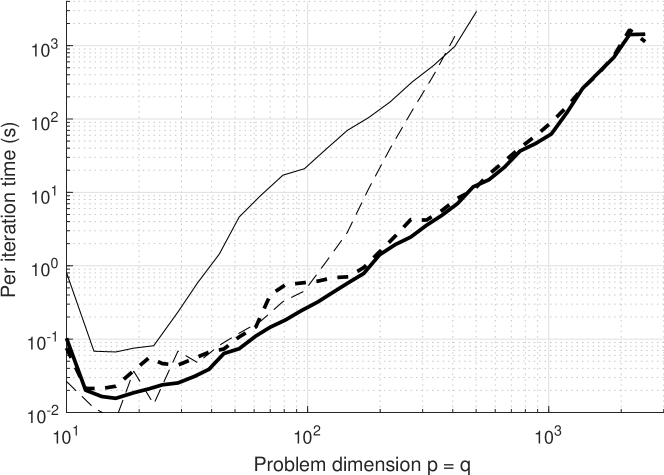
Figure 1: Per interior-point iteration time in seconds for modified SeDuMi (thick lines) and regular SeDuMi (thin lines) for matrix completion SDPs with $p=q$, rank $k=1$ and: (solid) $m=50p=25n$ constraints; (dashed) $m=0.1pq=0.025n^{2}$ constraints.

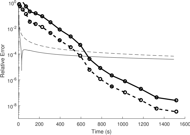
Figure 2: Progress of modified SeDuMi (thick lines) and singular value thresholding (thin lines) for a matrix completion problem with $p=q=500$, rank $k=4$, and $m=20,000$ constraints: (solid) objective error $\mathrm{abs}(\|Z\|_{*}-\|M\|_{*})/\|M\|_{*}$; (dashed) relative residual $\left(\sum_{i,j\in\Omega}(Z_{i,j}-M_{i,j})^{2}/\sum_{i,j\in\Omega}M_{i,j}^{2}\right)^{1/2}$. Each dot represents a single interior-point iteration.

We implemented the preconditioner in Section IV in MATLAB, and embedded it within SeDuMi version 1.3 [11]; the resulting solver is publicly available at

http://alum.mit.edu/www/ryz

SeDuMi is an NT-scaled strictly feasible path-following interior-point method, so we expect all of our theoretical results to hold. In fact, the original SeDuMi code already incorporates PCG in its solution of the Hessian equation, but the preconditioner is a numerically stabilized Cholesky factorization of the actual Hessian matrix $\mathbf{H}=\mathbf{A}^{T}\mathbf{D}\mathbf{A}$. Therefore, our only substantial modification is to replace this near-exact preconditioner with the spectral approximation $\hat{\mathbf{H}}$, implemented using the augmented system representation in (23). The LDL Cholesky factorization is computed using the ldl command in MATLAB, which calls the MA57 routine by Duff [36].

For a general SDP, the exact value of $k=\mathrm{rank}\,X^{\star}$ is unknown until after the problem has already been solved. In theory, our guarantees will continue to hold by setting the rank parameter to any upper-bound $k_{\max}=O(k)$, but in practice, the algorithm will run considerably faster using a less pessimistic value. Our implementation uses the spectrum of the scaling matrix $W$ to dynamically estimate a reasonable approximation $\tilde{k}\approx k$. More specifically, given an upper-bound $k_{\max}\geq k$ and an eigenvalue ratio $\eta$, we set $\tilde{k}$ as:

$$\tilde{k}=\max\{i\in\{0,1,\ldots,k_{\max}\}:\lambda_{i}(W)\geq\eta\lambda_{i+1}(W)\}.$$

The heuristic is inspired by Proposition 4: as the interior-point method progresses and the duality gap parameter $\mu\to 0^{+}$, the true value of $k$ causes the ratio $\lambda_{k}(W)/\lambda_{k+1}(W)\in\Theta(1/\mu)$ to tend to infinity. In other words, $\tilde{k}$ is guaranteed to converge to the true $k$ as the interior-point method progresses towards the solution.

V-A Test problem: Matrix completion

The matrix completion problem seeks to recover a low-rank size-$p\times q$ rectangular matrix $M$, by observing an incomplete subset of entries $M_{i,j}$ at $\{i,j\}\in\Omega$ and solving the convex optimization program

$$Z^{\star}=\text{ minimize }\|Z\|_{*}\text{ s.t. }Z_{i,j}=M_{i,j}\;\forall\{i,j\}\in\Omega,$$ (24)

where the nuclear norm $\|Z\|_{*}=\mathrm{tr}\,(Z^{T}Z)^{1/2}$ is the sum of the singular values. Note that (24) is a size $n=p+q$ semidefinite program over $m=|\Omega|$ constraints

minimize $$I\bullet X$$ (25)

subject to $$\frac{1}{2}\begin{bmatrix}0_{p}&E_{i,j}^{T}\\ E_{i,j}&0_{q}\end{bmatrix}\bullet X=M_{i,j}\;\forall\{i,j\}\in\Omega$$

$$\begin{bmatrix}U&Z^{T}\\ Z&V\end{bmatrix}=X\succeq 0,$$

where $E_{i,j}$ is an $p\times q$ matrix containing a single “1” at its $\{i,j\}$-th element. It is a famous result by Candes and Recht [3], later improved by Candes and Tao [2] that, when $M$ is low-rank and incoherent, and the number of samples satisfy $m\geq Cn(\log n)^{2}$ with some constant $C$, then all $pq$ elements of $M$ are exactly recovered by solving (24). In other words, the solution to (24) is precisely $Z^{\star}=M$.

Matrix completion makes an ideal test problem for the PCG procedure described in this paper, for the following reasons:

1. The solution rank $k=\mathrm{rank}\,X^{\star}$ is easily adjustable by controlling the rank of the original matrix $M$;

2. The SDP order $n=p+q$ and the number of constraints $m$ are easily adjustable by controlling the size of the original matrix $M$ and by modifying the number of observations $|\Omega|$;

3. The data matrix $\mathbf{A}=[\mathrm{vec}\,A_{1},\ldots,\mathrm{vec}\,A_{m}]$ is highly sparse, and always satisfies Assumption 2 by construction.

In this section, we consider random instances of (25). More specifically, we select $\Omega\subseteq\{1,\ldots,p\}\times\{1,\ldots,q\}$ uniformly at random from all subsets with cardinality $m$, and set $M=G_{1}G_{2}^{T}$, where $G_{1}\in\mathbb{R}^{p\times k}$ and $G_{2}\in\mathbb{R}^{q\times k}$ are selected i.i.d. from the standard Gaussian.

V-B Comparison with standard SeDuMi

The matrix completion SDP (25) is a challenging test problem for all standard interior-point solvers. The bottleneck is factoring the $m\times m$ fully-dense Hessian matrix $\mathbf{H}$, for worst-case complexities of $O(n^{6})$ time and $O(n^{4})$ memory. Chordal decomposition cannot be used to reduce these complexity figures, because the underlying graph does not have a bounded treewidth; see [37].

By comparison, our modified SeDuMi gains considerable efficiency by avoiding an explicit treatment of the Hessian matrix $\mathbf{H}$. In all of our numerical trials, the augmented system (23) associated with the preconditioner $\hat{\mathbf{H}}$ is highly sparse, and the algorithm’s bottleneck is the matrix-vector product $(W\otimes W)\mathrm{vec}\,X=\mathrm{vec}\,(WXW)$, as a part of the matrix-vector product with $\mathbf{H}$. These are realized as matrix-matrix products and evaluated using BLAS routines, so our MATLAB implementation should have a comparable level of performance to a hand-coded C/C++ implementation.

Figure 1 compares the per-iteration cost of our modified SeDuMi and the standard implementation, on a modest workstation with 16 GB of RAM and an Intel Xeon E5-2609 v4 CPU with eight 1.70 GHz cores. Two sets of problems were considered: one set with $m=25n$ and another with $m=0.025n^{2}$. As shown, the time complexity of standard SeDuMi is highly dependent upon the number of constraints $m$, but this dependency is essentially eliminated in the modified version. Standard SeDuMi was able to solve problems with $p+q=n\approx 800$ before running of memory. By contrast, our modified SeDuMi was able to solve matrix completion problems as large as $n=5024$ and $m=6.31\times 10^{5}$, in around 8 hours. Simply storing the associated Hessian matrix would have required 1,600 GB of memory, which is a hundred times what was available. In all of these trials, PCG converges to an iterate of sufficient accuracy in 15-25 iterations (except when stagnation occurs due to numerical issues).

V-C Comparison with singular value thresholding

Our modified SeDuMi is a true second-order method, because it converges at a linear rate, requiring $O(\log(1/\epsilon))$ iterations to produce an $\epsilon$-accurate solution. To make this distinction clear, we compare our modified SeDuMi method with the singular value thresholding (SVT) algorithm, a popular and widely-used first-order method for matrix-completion problems [38]. The SVT algorithm implicitly represents $Z$ in its low-rank factored form, and computes singular values using the Lanczos iteration; its per-iteration complexity is as low as $\sim mk$ time and $\sim nk+m$ memory. However, the method converges sublinearly in the worst-case, requiring $O(1/\epsilon)$ iterations to produce an $\epsilon$-accurate solution.

Figure 2 shows the progress of our modified SeDuMi and SVT over a 25 minute period, for a random matrix completion problem with $p=q=500$, rank $k=4$, and $m=2\times 10^{4}$ observations. After 20,000 iterations, SVT outputs an estimation of $M$ with relative error of $\approx 10^{-4}$. Indeed, SVT was able to compute an iterate of nearly this accuracy in just 2 minutes, but its sublinear convergence rate produces diminishing returns for the additional computation time. By contrast, modified SeDuMi converges linearly, gaining one decimal digit of accuracy every 3 minutes. After 18 outer interior-point iterations and 4233 inner PCG iterations, the method outputs an estimation of $M$ with relative error of $\approx 10^{-8}$.

VI Conclusion

This paper describes a preconditioner that allows preconditioned conjugate gradients (PCG) to converge to a solution of the interior-point Hessian equation in a few tens of iterations, independent of the ill-conditioning of the Hessian matrix. The preconditioner can be factored in $\Theta(n^{3}k^{3})$ time and $\Theta(n^{2}k^{2})$ memory, and the cost of the subsequent PCG iterations is dominated by matrix-vector products with the Hessian matrix. We embed the preconditioner within SeDuMi, and use it to solve large-and-sparse, low-rank, matrix completion SDPs to 8-10 decimal digits of accuracy. The largest problem we considered had $n=5024$ and $m=6.31\times 10^{5}$, and was solved in less than 8 hours on a modest workstation with 16 GB of memory.

References

- [1] S. Sojoudi and J. Lavaei, “Exactness of semidefinite relaxations for nonlinear optimization problems with underlying graph structure,” SIAM Journal on Optimization, vol. 24, no. 4, pp. 1746–1778, 2014.
- [2] E. J. Candès and T. Tao, “The power of convex relaxation: Near-optimal matrix completion,” IEEE Transactions on Information Theory, vol. 56, no. 5, pp. 2053–2080, 2010.
- [3] E. Candès and B. Recht, “Exact matrix completion via convex optimization,” Communications of the ACM, vol. 55, no. 6, pp. 111–119, 2012.
- [4] J. B. Lasserre, Moments, positive polynomials and their applications. World Scientific, 2009, vol. 1.
- [5] G. Valmorbida, M. Ahmadi, and A. Papachristodoulou, “Stability analysis for a class of partial differential equations via semidefinite programming,” IEEE Transactions on Automatic Control, vol. 61, no. 6, pp. 1649–1654, 2016.
- [6] R. Y. Zhang, “Robust stability analysis for large-scale power systems,” Ph.D. dissertation, Massachusetts Institute of Technology, 2016.
- [7] R. Madani, A. Kalbat, and J. Lavaei, “ADMM for sparse semidefinite programming with applications to optimal power flow problem,” in IEEE 54th Annual Conference on Decision and Control (CDC) 2015. IEEE, 2015, pp. 5932–5939.
- [8] R. Madani, S. Sojoudi, and J. Lavaei, “Convex relaxation for optimal power flow problem: Mesh networks,” IEEE Transactions on Power Systems, vol. 30, no. 1, pp. 199–211, 2015.
- [9] P. A. Parrilo, “Semidefinite programming relaxations for semialgebraic problems,” Mathematical programming, vol. 96, no. 2, pp. 293–320, 2003.
- [10] F. Alizadeh, J.-P. A. Haeberly, and M. L. Overton, “Complementarity and nondegeneracy in semidefinite programming,” Mathematical Programming, vol. 77, no. 1, pp. 111–128, 1997.
- [11] J. F. Sturm, “Using SeDuMi 1.02, a MATLAB toolbox for optimization over symmetric cones,” Optimization methods and software, vol. 11, no. 1-4, pp. 625–653, 1999.
- [12] MOSEK ApS, The MOSEK optimization toolbox for MATLAB manual. Version 7.1 (Revision 28)., 2015. [Online]. Available: http://docs.mosek.com/7.1/toolbox/index.html
- [13] Y. Ye, M. J. Todd, and S. Mizuno, “An -iteration homogeneous and self-dual linear programming algorithm,” Mathematics of Operations Research, vol. 19, no. 1, pp. 53–67, 1994.
- [14] Z. Wen, D. Goldfarb, and W. Yin, “Alternating direction augmented lagrangian methods for semidefinite programming,” Mathematical Programming Computation, vol. 2, no. 3-4, pp. 203–230, 2010.
- [15] A. Kalbat and J. Lavaei, “A fast distributed algorithm for decomposable semidefinite programs,” in IEEE 54th Annual Conference on Decision and Control (CDC) 2015. IEEE, 2015, pp. 1742–1749.
- [16] B. O’Donoghue, E. Chu, N. Parikh, and S. Boyd, “Conic optimization via operator splitting and homogeneous self-dual embedding,” Journal of Optimization Theory and Applications, vol. 169, no. 3, pp. 1042–1068, 2016.
- [17] R. Y. Zhang and J. K. White, “On the convergence of GMRES-accelerated ADMM in iterations for quadratic objectives,” arXiv preprint arXiv:1601.06200, 2016.
- [18] K.-C. Toh and M. Kojima, “Solving some large scale semidefinite programs via the conjugate residual method,” SIAM Journal on Optimization, vol. 12, no. 3, pp. 669–691, 2002.
- [19] X.-Y. Zhao, D. Sun, and K.-C. Toh, “A Newton-CG augmented lagrangian method for semidefinite programming,” SIAM Journal on Optimization, vol. 20, no. 4, pp. 1737–1765, 2010.
- [20] M. Fukuda, M. Kojima, K. Murota, and K. Nakata, “Exploiting sparsity in semidefinite programming via matrix completion I: General framework,” SIAM Journal on Optimization, vol. 11, no. 3, pp. 647–674, 2001.
- [21] L. Vandenberghe, M. S. Andersen et al., “Chordal graphs and semidefinite optimization,” Foundations and Trends in Optimization, vol. 1, no. 4, pp. 241–433, 2015.
- [22] S. Kim, M. Kojima, M. Mevissen, and M. Yamashita, “Exploiting sparsity in linear and nonlinear matrix inequalities via positive semidefinite matrix completion,” Mathematical programming, vol. 129, no. 1, pp. 33–68, 2011.
- [23] S. Burer and R. D. Monteiro, “A nonlinear programming algorithm for solving semidefinite programs via low-rank factorization,” Mathematical Programming, vol. 95, no. 2, pp. 329–357, 2003.
- [24] M. Journée, F. Bach, P.-A. Absil, and R. Sepulchre, “Low-rank optimization on the cone of positive semidefinite matrices,” SIAM Journal on Optimization, vol. 20, no. 5, pp. 2327–2351, 2010.
- [25] S. J. Wright, Primal-dual interior-point methods. SIAM, 1997.
- [26] S. Boyd and L. Vandenberghe, Convex optimization. Cambridge university press, 2004.
- [27] R. Barrett, M. Berry, T. F. Chan, J. Demmel, J. Donato, J. Dongarra, V. Eijkhout, R. Pozo, C. Romine, and H. Van der Vorst, Templates for the solution of linear systems: building blocks for iterative methods. SIAM, 1994.
- [28] A. Greenbaum, Iterative methods for solving linear systems. SIAM, 1997.
- [29] Y. Nesterov and A. Nemirovskii, Interior-point polynomial algorithms in convex programming. SIAM, 1994.
- [30] L. Vandenberghe, S. Boyd, and S.-P. Wu, “Determinant maximization with linear matrix inequality constraints,” SIAM journal on matrix analysis and applications, vol. 19, no. 2, pp. 499–533, 1998.
- [31] T. Ando, “Concavity of certain maps on positive definite matrices and applications to hadamard products,” Linear Algebra and its Applications, vol. 26, pp. 203–241, 1979.
- [32] J. E. Mitchell, P. M. Pardalos, and M. G. Resende, “Interior point methods for combinatorial optimization,” in Handbook of combinatorial optimization. Springer, 1998, pp. 189–297.
- [33] R. H. Byrd, M. E. Hribar, and J. Nocedal, “An interior point algorithm for large-scale nonlinear programming,” SIAM Journal on Optimization, vol. 9, no. 4, pp. 877–900, 1999.
- [34] M. Benzi, G. H. Golub, and J. Liesen, “Numerical solution of saddle point problems,” Acta numerica, vol. 14, pp. 1–137, 2005.
- [35] E. Yip, “A note on the stability of solving a rank-p modification of a linear system by the sherman–morrison–woodbury formula,” SIAM Journal on Scientific and Statistical Computing, vol. 7, no. 2, pp. 507–513, 1986.
- [36] I. S. Duff, “MA57—a code for the solution of sparse symmetric definite and indefinite systems,” ACM Transactions on Mathematical Software (TOMS), vol. 30, no. 2, pp. 118–144, 2004.
- [37] Y. Gao, “Treewidth of Erdos–Renyi random graphs, random intersection graphs, and scale-free random graphs,” Discrete Applied Mathematics, vol. 160, no. 4, pp. 566–578, 2012.
- [38] J.-F. Cai, E. J. Candès, and Z. Shen, “A singular value thresholding algorithm for matrix completion,” SIAM Journal on Optimization, vol. 20, no. 4, pp. 1956–1982, 2010.