Ultrasensitivity and Fluctuations in the Barkai-Leibler Model of Chemotaxis Receptors in Escherichia coli

Ushasi Roy*, Manoj Gopalakrishnan✝

Department of Physics, Indian Institute of Technology Madras,
Chennai, Tamil Nadu, India

* ushasi@physics.iitm.ac.in
βœβ€„ manojgopal@iitm.ac.in
Abstract

A stochastic version of the Barkai-Leibler model of chemotaxis receptors in Escherichia coli is studied here with the goal of elucidating the effects of intrinsic network noise in their conformational dynamics. The model was originally proposed to explain the robust and near-perfect adaptation of E. coli observed across a wide range of spatially uniform attractant/repellent (ligand) concentrations. In the model, a receptor is either active or inactive and can stochastically switch between the two states. The enzyme CheR methylates inactive receptors while CheB demethylates active receptors and the probability for a receptor to be active depends on its level of methylation and ligand occupation. In a simple version of the model with two methylation sites per receptor (M=2𝑀2M=2), we show rigorously, under a quasi-steady state approximation, that the mean active fraction of receptors is an ultrasensitive function of [CheR]/[CheB] in the limit of saturating receptor concentration. Hence the model shows zero-order ultrasensitivity (ZOU), similar to the classical two-state model of covalent modification studied by Goldbeter and Koshland (GK). We also find that in the limits of extremely small and extremely large ligand concentrations, the system reduces to two different two-state GK modules. A quantitative measure of the spontaneous fluctuations in activity is provided by the variance Οƒa2superscriptsubscriptπœŽπ‘Ž2\sigma_{a}^{2} in the active fraction, which is estimated mathematically under linear noise approximation (LNA). It is found that Οƒa2superscriptsubscriptπœŽπ‘Ž2\sigma_{a}^{2} peaks near the ZOU transition. The variance is a non-monotonic, but weak function of ligand concentration and a decreasing function of receptor concentration. Gillespie simulations are also performed in models with M=2,3𝑀23M=2,3 and 4. For M=2𝑀2M=2, simulations show excellent agreement with analytical results obtained under LNA. Numerical results for M=3𝑀3M=3 and M=4𝑀4M=4 are qualitatively similar to our mathematical results in M=2𝑀2M=2; while all the models show ZOU in mean activity, the variance is found to be smaller for larger M𝑀M. The magnitude of receptor noise deduced from available experimental data is consistent with our predictions. A simple analysis of the downstream signaling pathway shows that this noise is large enough to affect the motility of the organism, and may have a beneficial effect on it. The response of mean receptor activity to small time-dependent changes in the external ligand concentration is computed within linear response theory, and found to have a bilobe form, in agreement with earlier experimental observations.

1 Introduction

The pioneering work [1] of Goldbeter and Koshland (GK) brought into light an interesting molecular switch-like transition, now referred to as Zero Order Ultrasensitivity (ZOU) [2], observed in reversible covalent modification (e.g. phosphorylation or methylation) of a protein (substrate), catalyzed by two antagonistic enzymes. This switch-like behavior emerges in the limit where the substrate concentration is exceedingly large compared to the enzyme concentrations as well as their individual Michaelis constants. In this β€œzero-order” regime, the modified fraction of substrate, in a saturating environment, exhibits a sharp transition at a critical value of the ratio of the total concentrations of the antagonistic enzymes. Various aspects of GK switch has been studied over the years [3, 4, 5]. The fluctuations associated with the ultrasensitive module has also been studied [3, 4]. ZOU was also identified as allosteric cooperativity by Quian (2003) [6] and Ge and Quian (2008) [7].

The bacterium E. coli has thousands of receptors on its cell surface for a precise sensation of the extracellular environment. The two main types of chemotaxis receptors are Tar and Tsr. The receptor protein and the protein kinase CheA are linked by the linker protein CheW. The receptor protein, CheA and CheW function as a single signaling complex, which exists in active or inactive state, and can undergo stochastic switching between the states. The switching is regulated by methylation and ligandation (binding of chemoattractant/repellent) of the receptors. Methylation is carried out by the protein CheR while CheB demethylates receptors. In its active state, the receptor-CheW-CheA complex phosphorylates CheB and the response regulator CheY; while the former demethylates the receptor, the latter induces tumbles by binding to the flagellar motor. In this way, the internal biochemistry (methylation/demethylation) and external stimulus (attractant/repellent) regulates the swimming pattern of the organism (reviewed in [8]).

A remarkable property of chemotaxis in E. coli is perfect adaptation to some chemoattractants. After exposure to a stimulus corresponding to an abrupt rise or fall in ligand concentration in a homogeneous environment, the frequency of tumbles returns to its pre-stimulus level after a time interval ∼similar-to\sim 4 seconds [9]. A model of the methylation-demethylation cascade proposed by Barkai and Leibler (BL) [10] successfully explains this property using a few simple assumptions. The model was modified and extended in later years by other authors [11, 12, 13, 14]. The important assumptions in the model are (a) CheR methylates inactive receptors while CheB (or its phosphorylated form, CheBp) demethylates active receptors, (b) the state of activity of a receptor depends on its methylation level, (c) binding of an attractant (ligand) molecule adversely affects the activity of a receptor, (d) ligand binding and dissociation are very fast compared to methylation and demethylation. Mello and Tu [13] showed that perfect adaptation is achieved only if the lowest methylation level is assumed to be always inactive, while the highest level is assumed to be always active. As a consequence of these assumptions, the mean receptor activity in the model in steady state turns out to be independent of the attractant concentration. Further, mathematical modeling has shown that, with suitable extensions, the model also successfully predicts the response of the network to a short-lived spike in attractant concentration[15].

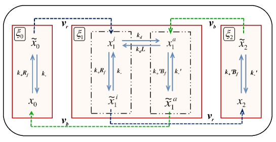
In E.coli, the most abundant receptor, Tar, responding to the attractant methyl aspartate, has four methylation sites per monomer. For modeling purposes, it is convenient to represent the methylation state of a single receptor by an index mπ‘šm, where 0≀m≀M0π‘šπ‘€0\leq m\leq M with M𝑀M being the maximum value (M=4𝑀4M=4 for Tar). It is generally assumed that activation/inactivation as well as ligand binding/unbinding of a receptor happens much faster compared to methylation/demethylation. For M=1𝑀1M=1, the BL model is entirely identical with the Goldbeter-Koshland (GK) two-state system; the ligand concentration L𝐿L plays no role whatsoever in the dynamics. For Mβ‰₯2𝑀2M\geq 2, the intermediate state(s) which stochastically switches(switch) between active and inactive states modifies the dynamics; however, the model retains the same structure as the GK module (see Fig 1, where we have provided a schematic depiction of the BL model, for M=2𝑀2M=2). Therefore, it is pertinent to enquire whether ZOU is present also in the BL model. In the GK system (M=2𝑀2M=2 in our model), fluctuations in activity are known to be large near the ZOU transition. In E.coli chemotaxis, intrinsic fluctuations are expected to play an important role. The flagellar motor responds ultrasensitively to [CheYp] (p denoting the phosphorylated form); the sensitive part of the motor response curve is less than 1ΞΌπœ‡\muM in width [17, 16], hence it is likely that spontaneous and random fluctuations in activity are crucial in generating the run-and-tumble motion of the organism [12]. For this reason, we believe that a detailed study of ZOU in the BL model, including a systematic treatment of fluctuations will make a useful addition to existing literature on ZOU as well as chemotaxis in E.coli. This is the motivation behind this paper.
Refer to caption
Figure 1: A schematic figure of the 3-state BL Model showing all the biochemical reactions. The red boxes denote the three states; ΞΎ0subscriptπœ‰0\xi_{0}, ΞΎ1subscriptπœ‰1\xi_{1} and ΞΎ2subscriptπœ‰2\xi_{2} being the fractional concentrations of receptors in each. Blue dotted arrows with rates Ξ½rsubscriptπœˆπ‘Ÿ\nu_{r} show the methylation process resulting in the increment in the state index while the green ones with rates Ξ½bsubscriptπœˆπ‘\nu_{b} depict demethylation with the decrement in the same.

2 Materials and Methods

2.1 Model details

Let us denote by V𝑉V the volume of a cell having a total of N=A0​V𝑁subscript𝐴0𝑉N=A_{0}V receptor proteins (substrate), and two enzymes. In E.coli, these correspond to the methyltransferase CheR and methylesterase CheB, the total concentrations of each are denoted by R0subscript𝑅0R_{0} and B0subscript𝐡0B_{0} respectively. In the presently accepted model of signal transduction in E.coli, CheR methylates the receptor, while CheB demethylates it. According to the two-state model [18] the receptor exists in a complex form involving two more proteins, CheW and CheA, and the complex may exist in one of two conformational states, which we refer to as active and inactive. In the active state, CheA undergoes autophosphorylation and also phosphorylates the cytoplasmic messenger protein CheY. CheA phosphorylates CheB also, a process crucial in adaptation, but ignored here for the sake of maintaining close structural similarity with the GK system. The probability to be in the active state is an increasing function of the methylation level of the receptor. Chemoattractant molecules, if present, also bind to the receptor, and this process increases the probability to find the receptor in inactive state (with chemorepellents, it is the reverse)[8].

BL proposed a quantitative model [10] of the signal transduction cascade, based on the two-state model of Asakura and Honda [18]. In this model, CheR binds only to inactive receptors, while CheB binds only to active receptors [19]. In general, we denote by M𝑀M the total number of methylation sites. Let Amsubscriptπ΄π‘šA_{m} symbolically represent a receptor in methylation state mπ‘šm, and A~msubscript~π΄π‘š\tilde{A}_{m} denotes its enzyme-bound form; the same symbols will also be used to denote the corresponding numbers (out of a total of N𝑁N). The inactive and active versions are identified by superscripts i𝑖i and aπ‘Ža respectively. The binding rate of CheR to a receptor is k+subscriptπ‘˜k_{+} and kβˆ’subscriptπ‘˜k_{-} is the dissociation rate; for CheB, the corresponding quantities are k+β€²superscriptsubscriptπ‘˜β€²k_{+}^{\prime} and kβˆ’β€²superscriptsubscriptπ‘˜β€²k_{-}^{\prime} respectively. Attractant binding is relevant only for the intermediate state; we assume that the binding rate is kasubscriptπ‘˜π‘Žk_{a}, dissociation rate is kdsubscriptπ‘˜π‘‘k_{d} and attractant concentration is L𝐿L (assumed uniform). Ξ½rsubscriptπœˆπ‘Ÿ\nu_{r} and Ξ½bsubscriptπœˆπ‘\nu_{b} represent the product formation rates from CheR and CheB-bound intermediate states, respectively. The concentrations of the free forms of CheR and CheB are denoted by Rfsubscript𝑅𝑓R_{f} and Bfsubscript𝐡𝑓B_{f} respectively. We also define a set of dissociation constants: Kr=kβˆ’/k+,Kb=kβˆ’β€²/k+β€²,KL=kd/kaformulae-sequencesubscriptπΎπ‘Ÿsubscriptπ‘˜subscriptπ‘˜formulae-sequencesubscript𝐾𝑏superscriptsubscriptπ‘˜β€²superscriptsubscriptπ‘˜β€²subscript𝐾𝐿subscriptπ‘˜π‘‘subscriptπ‘˜π‘ŽK_{r}=k_{-}/k_{+},K_{b}=k_{-}^{\prime}/k_{+}^{\prime},K_{L}=k_{d}/k_{a}.

If ΞΎm​(t)subscriptπœ‰π‘šπ‘‘\xi_{m}(t) denote the fraction of receptors in methylation state mπ‘šm at time t𝑑t, the total active fraction of receptors is given by ΞΎa​(t)=βˆ‘m=0Mam​(L)​ξm​(t)subscriptπœ‰π‘Žπ‘‘superscriptsubscriptπ‘š0𝑀subscriptπ‘Žπ‘šπΏsubscriptπœ‰π‘šπ‘‘\xi_{a}(t)=\sum_{m=0}^{M}a_{m}(L)\xi_{m}(t), where am​(L)subscriptπ‘Žπ‘šπΏa_{m}(L) is the probability for a receptor in state mπ‘šm to be active, L𝐿L being the (uniform) attractant concentration. We assume that the lowest state (m=0π‘š0m=0) is always inactive, while m=Mπ‘šπ‘€m=M is always active; the intermediate state(s) can be either active or inactive, depending on whether it is attractant-bound. A simple mathematical form satisfying these conditions is am​(L)=am​(0)​Km/(L+Km)subscriptπ‘Žπ‘šπΏsubscriptπ‘Žπ‘š0subscriptπΎπ‘šπΏsubscriptπΎπ‘ša_{m}(L)=a_{m}(0)K_{m}/(L+K_{m}) where KmsubscriptπΎπ‘šK_{m} is the dissociation constant for attractant binding to a receptor in state mπ‘šm [20, 14, 15]. To satisfy the earlier assumption, we choose K0=0subscript𝐾00K_{0}=0 and KM=∞subscript𝐾𝑀K_{M}=\infty (these are ideal values). We further choose am0=m/Msuperscriptsubscriptπ‘Žπ‘š0π‘šπ‘€a_{m}^{0}=m/M[19], a simple mathematical form which satisfies our earlier assumptions.

2.2 Fokker-Planck equation for M=2𝑀2M=2

We will first carry out a detailed mathematical analysis of the properties of the BL model with M=2𝑀2M=2. Fig 1 shows a schematic depiction of this case, showing all the biochemical reactions. In the limit where the modification rates Ξ½rsubscriptπœˆπ‘Ÿ\nu_{r} and Ξ½bsubscriptπœˆπ‘\nu_{b} are very small in comparison with the other rates, it may be visualized as a combination of three weakly-coupled modules (the boxes in FigΒ 1); the fractional populations of receptors in each module are ΞΎmsubscriptπœ‰π‘š\xi_{m} with m=0,1,2π‘š012m=0,1,2; hence βˆ‘m=02ΞΎm=1superscriptsubscriptπ‘š02subscriptπœ‰π‘š1\sum_{m=0}^{2}\xi_{m}=1. In general, for a complete stochastic description of the dynamics of this system, we also need to keep track of time evolution of the intra-modular populations viz., xmsubscriptπ‘₯π‘šx_{m} and x~msubscript~π‘₯π‘š{\tilde{x}}_{m}. For m=1π‘š1m=1, there is a further sub-division: x1=x1a+x1isubscriptπ‘₯1superscriptsubscriptπ‘₯1π‘Žsuperscriptsubscriptπ‘₯1𝑖x_{1}=x_{1}^{a}+x_{1}^{i} and x~1=x~1a+x~1isubscript~π‘₯1superscriptsubscript~π‘₯1π‘Žsuperscriptsubscript~π‘₯1𝑖{\tilde{x}}_{1}={\tilde{x}}_{1}^{a}+{\tilde{x}}_{1}^{i}, as explained in the previous section. For each mπ‘šm, ΞΎm=xm+x~msubscriptπœ‰π‘šsubscriptπ‘₯π‘šsubscript~π‘₯π‘š\xi_{m}=x_{m}+{\tilde{x}}_{m}. It was shown by us in an earlier paper [2] that these intra-modular fractions can be β€˜integrated out’ using one of the quasi-steady state approximation schemes (QSSA) [21], whereby the replacement xiβ†’xi¯​(𝝃)β†’subscriptπ‘₯𝑖¯subscriptπ‘₯𝑖𝝃x_{i}\to\overline{x_{i}}(\boldsymbol{\xi}) naturally appears in the relevant inter-modular conversion rates. Here, we have introduced the compact vector symbol 𝝃≑(ΞΎ0,ΞΎ2)𝝃subscriptπœ‰0subscriptπœ‰2\boldsymbol{\xi}\equiv(\xi_{0},\xi_{2}) (because of the normalization constraint mentioned above, only two of the fractions ΞΎmsubscriptπœ‰π‘š\xi_{m} are independent, we shall take these to be ΞΎ0subscriptπœ‰0\xi_{0} and ΞΎ2subscriptπœ‰2\xi_{2} purely for reasons of convenience).

Therefore, within this approximation, the inter-modular dynamics may be expressed in terms of a probability density P​(𝝃;t)𝑃𝝃𝑑P(\boldsymbol{\xi};t), which satisfies a non-linear Fokker-Planck equation (FPE) in the form of a local equation of continuity[2]:

βˆ‚P​(𝝃,t)βˆ‚t=βˆ’βˆ‚βˆ‚πƒβ‹…π‰π‘ƒπƒπ‘‘π‘‘β‹…πƒπ‰\frac{\partial P(\boldsymbol{\xi},t)}{\partial t}=-\frac{\partial}{\partial\boldsymbol{\xi}}\cdot\bf{J} (1)

where J≑{J0,J2}Jsubscript𝐽0subscript𝐽2\textbf{J}\equiv\{J_{0},J_{2}\} with Jm=vm​Pβˆ’βˆ‚βˆ‚ΞΎm​(Dm​P)subscriptπ½π‘šsubscriptπ‘£π‘šπ‘ƒsubscriptπœ‰π‘šsubscriptπ·π‘šπ‘ƒJ_{m}=v_{m}P-\frac{\partial}{\partial\xi_{m}}(D_{m}P) (for m=0,2π‘š02m=0,2) denoting the components of the state space probability current β€œvector”. Here, the drift and diffusion coefficients are given by

vm=δ​(Ο‰1​mβˆ’Ο‰m​1);Dm=Ξ΄22​(Ο‰1​m+Ο‰m​1);m=0,2formulae-sequencesubscriptπ‘£π‘šπ›Ώsubscriptπœ”1π‘šsubscriptπœ”π‘š1formulae-sequencesubscriptπ·π‘šsuperscript𝛿22subscriptπœ”1π‘šsubscriptπœ”π‘š1π‘š02v_{m}=\delta(\omega_{1m}-\omega_{m1})~{}~{};~{}~{}~{}D_{m}=\frac{\delta^{2}}{2}(\omega_{1m}+\omega_{m1})~{}~{};~{}~{}~{}m=0,2 (2)

with Ξ΄=Nβˆ’1𝛿superscript𝑁1\delta=N^{-1}, Ο‰10=N​νb​x~1asubscriptπœ”10𝑁subscriptπœˆπ‘superscriptsubscript~π‘₯1π‘Ž\omega_{10}=N\nu_{b}\tilde{x}_{1}^{a}, Ο‰01=N​νr​x~0subscriptπœ”01𝑁subscriptπœˆπ‘Ÿsubscript~π‘₯0\omega_{01}=N\nu_{r}\tilde{x}_{0}, Ο‰12=N​νr​x~1isubscriptπœ”12𝑁subscriptπœˆπ‘Ÿsuperscriptsubscript~π‘₯1𝑖\omega_{12}=N\nu_{r}\tilde{x}_{1}^{i} and Ο‰21=N​νb​x~2subscriptπœ”21𝑁subscriptπœˆπ‘subscript~π‘₯2\omega_{21}=N\nu_{b}\tilde{x}_{2}.

Incorporating the rates Ο‰m​nsubscriptπœ”π‘šπ‘›\omega_{mn} in the above expressions for vmsubscriptπ‘£π‘šv_{m} and Dmsubscriptπ·π‘šD_{m} and employing the inter-module dynamics under the standard quasi-steady state approximation (sQSSA) as discussed in 6.1, we arrive at the following expressions for the drift and diffusion coefficients:

v0​(𝝃)subscript𝑣0𝝃\displaystyle v_{0}(\boldsymbol{\xi}) =\displaystyle= Ξ½b​BfBf+Kb​(KLL+KL)​(1βˆ’ΞΎ0βˆ’ΞΎ2)βˆ’Ξ½r​RfRf+Kr​ξ0,subscriptπœˆπ‘subscript𝐡𝑓subscript𝐡𝑓subscript𝐾𝑏subscript𝐾𝐿𝐿subscript𝐾𝐿1subscriptπœ‰0subscriptπœ‰2subscriptπœˆπ‘Ÿsubscript𝑅𝑓subscript𝑅𝑓subscriptπΎπ‘Ÿsubscriptπœ‰0\displaystyle\frac{\nu_{b}B_{f}}{B_{f}+K_{b}}\left(\frac{K_{L}}{L+K_{L}}\right)(1-\xi_{0}-\xi_{2})-\frac{\nu_{r}R_{f}}{R_{f}+K_{r}}\xi_{0},
v2​(𝝃)subscript𝑣2𝝃\displaystyle v_{2}(\boldsymbol{\xi}) =\displaystyle= Ξ½r​RfRf+Kr​(LL+KL)​(1βˆ’ΞΎ0βˆ’ΞΎ2)βˆ’Ξ½b​BfBf+Kb​ξ2,subscriptπœˆπ‘Ÿsubscript𝑅𝑓subscript𝑅𝑓subscriptπΎπ‘ŸπΏπΏsubscript𝐾𝐿1subscriptπœ‰0subscriptπœ‰2subscriptπœˆπ‘subscript𝐡𝑓subscript𝐡𝑓subscript𝐾𝑏subscriptπœ‰2\displaystyle\frac{\nu_{r}R_{f}}{R_{f}+K_{r}}\left(\frac{L}{L+K_{L}}\right)(1-\xi_{0}-\xi_{2})-\frac{\nu_{b}B_{f}}{B_{f}+K_{b}}\xi_{2}, (3)

and

D0​(𝝃)subscript𝐷0𝝃\displaystyle D_{0}(\boldsymbol{\xi}) =\displaystyle= 12​N​[Ξ½b​BfBf+Kb​(KLL+KL)​(1βˆ’ΞΎ0βˆ’ΞΎ2)+Ξ½r​RfRf+Kr​ξ0],12𝑁delimited-[]subscriptπœˆπ‘subscript𝐡𝑓subscript𝐡𝑓subscript𝐾𝑏subscript𝐾𝐿𝐿subscript𝐾𝐿1subscriptπœ‰0subscriptπœ‰2subscriptπœˆπ‘Ÿsubscript𝑅𝑓subscript𝑅𝑓subscriptπΎπ‘Ÿsubscriptπœ‰0\displaystyle\frac{1}{2N}\Bigg{[}\frac{\nu_{b}B_{f}}{B_{f}+K_{b}}\left(\frac{K_{L}}{L+K_{L}}\right)(1-\xi_{0}-\xi_{2})+\frac{\nu_{r}R_{f}}{R_{f}+K_{r}}\xi_{0}\Bigg{]},
D2​(𝝃)subscript𝐷2𝝃\displaystyle D_{2}(\boldsymbol{\xi}) =\displaystyle= 12​N​[Ξ½r​RfRf+Kr​(LL+KL)​(1βˆ’ΞΎ0βˆ’ΞΎ2)+Ξ½b​BfBf+Kb​ξ2].12𝑁delimited-[]subscriptπœˆπ‘Ÿsubscript𝑅𝑓subscript𝑅𝑓subscriptπΎπ‘ŸπΏπΏsubscript𝐾𝐿1subscriptπœ‰0subscriptπœ‰2subscriptπœˆπ‘subscript𝐡𝑓subscript𝐡𝑓subscript𝐾𝑏subscriptπœ‰2\displaystyle\frac{1}{2N}\Bigg{[}\frac{\nu_{r}R_{f}}{R_{f}+K_{r}}\left(\frac{L}{L+K_{L}}\right)(1-\xi_{0}-\xi_{2})+\frac{\nu_{b}B_{f}}{B_{f}+K_{b}}\xi_{2}\Bigg{]}. (4)

The free enzyme concentrations Rfsubscript𝑅𝑓R_{f} and Bfsubscript𝐡𝑓B_{f} are also functions of ΞΎ0,ΞΎ2subscriptπœ‰0subscriptπœ‰2\xi_{0},\xi_{2}, and the expressions are given by (see 6.1)

Rf​(𝝃)subscript𝑅𝑓𝝃\displaystyle R_{f}(\boldsymbol{\xi}) =\displaystyle= R0​Kr​(L+KL)Kr​(L+KL)+A0​[KL​ξ0+L​(1βˆ’ΞΎ2)],subscript𝑅0subscriptπΎπ‘ŸπΏsubscript𝐾𝐿subscriptπΎπ‘ŸπΏsubscript𝐾𝐿subscript𝐴0delimited-[]subscript𝐾𝐿subscriptπœ‰0𝐿1subscriptπœ‰2\displaystyle\frac{R_{0}K_{r}(L+K_{L})}{K_{r}(L+K_{L})+A_{0}[K_{L}\xi_{0}+L(1-\xi_{2})]}~{},
Bf​(𝝃)subscript𝐡𝑓𝝃\displaystyle B_{f}(\boldsymbol{\xi}) =\displaystyle= B0​Kb​(L+KL)Kb​(L+KL)+A0​[KL​(1βˆ’ΞΎ0)+L​ξ2].subscript𝐡0subscript𝐾𝑏𝐿subscript𝐾𝐿subscript𝐾𝑏𝐿subscript𝐾𝐿subscript𝐴0delimited-[]subscript𝐾𝐿1subscriptπœ‰0𝐿subscriptπœ‰2\displaystyle\frac{B_{0}K_{b}(L+K_{L})}{K_{b}(L+K_{L})+A_{0}[K_{L}(1-\xi_{0})+L\xi_{2}]}~{}. (5)

3 Results

3.1 Averages as fixed points

From (1), it is seen after the required averaging that the time evolution of the mean receptor fractions is given by the vector equation

d​ξ¯d​t=𝐯​(𝝃)Β―,π‘‘Β―πœ‰π‘‘π‘‘Β―π―πƒ\frac{d\overline{\bf{\xi}}}{dt}=\overline{\bf{v}(\boldsymbol{\xi})}, (6)

where 𝐯​(𝝃)≑(v0​(𝝃),v2​(𝝃))𝐯𝝃subscript𝑣0𝝃subscript𝑣2𝝃{\bf v}(\boldsymbol{\xi})\equiv(v_{0}(\boldsymbol{\xi}),v_{2}(\boldsymbol{\xi})) is the drift β€œvector”. In general, this vector vanishes at one or more points in the (ΞΎ0,ΞΎ2)subscriptπœ‰0subscriptπœ‰2(\xi_{0},\xi_{2}) space; following van Kampen[22], we shall refer to this point (assuming only one exists) as the fixed point, denoted πƒβˆ—=(ΞΎ0βˆ—,ΞΎ2βˆ—)superscript𝝃superscriptsubscriptπœ‰0superscriptsubscriptπœ‰2\boldsymbol{\xi}^{*}=(\xi_{0}^{*},\xi_{2}^{*}). It can be shown (see later) that in the large N𝑁N-limit, the fixed point becomes identical to the mean value ΞΎΒ―Β―πœ‰\overline{{\bf\xi}}.

Under conditions Rfβ‰ͺKrmuch-less-thansubscript𝑅𝑓subscriptπΎπ‘ŸR_{f}\ll K_{r} and Bfβ‰ͺKbmuch-less-thansubscript𝐡𝑓subscript𝐾𝑏B_{f}\ll K_{b}, which we shall assume to hold for reasons of simplicity, it follows from (2.2) that the fixed point is given by

ΞΎ0βˆ—=Bfβˆ—2​Kr2​νb2​KL(Bfβˆ—β€‹Kr​νb+Rfβˆ—β€‹Kb​νr)​(Bfβˆ—β€‹Kr​νb​KL+Rfβˆ—β€‹Kb​νr​L)superscriptsubscriptπœ‰0superscriptsubscript𝐡𝑓absent2superscriptsubscriptπΎπ‘Ÿ2superscriptsubscriptπœˆπ‘2subscript𝐾𝐿superscriptsubscript𝐡𝑓subscriptπΎπ‘Ÿsubscriptπœˆπ‘superscriptsubscript𝑅𝑓subscript𝐾𝑏subscriptπœˆπ‘Ÿsuperscriptsubscript𝐡𝑓subscriptπΎπ‘Ÿsubscriptπœˆπ‘subscript𝐾𝐿superscriptsubscript𝑅𝑓subscript𝐾𝑏subscriptπœˆπ‘ŸπΏ\displaystyle\xi_{0}^{*}=\frac{B_{f}^{*2}K_{r}^{2}\nu_{b}^{2}K_{L}}{(B_{f}^{*}K_{r}\nu_{b}+R_{f}^{*}K_{b}\nu_{r})(B_{f}^{*}K_{r}\nu_{b}K_{L}+R_{f}^{*}K_{b}\nu_{r}L)}
ΞΎ2βˆ—=Rfβˆ—2​Kb2​νr2​L(Bfβˆ—β€‹Kr​νb+Rfβˆ—β€‹Kb​νr)​(Bfβˆ—β€‹Kr​νb​KL+Rfβˆ—β€‹Kb​νr​L),superscriptsubscriptπœ‰2superscriptsubscript𝑅𝑓absent2superscriptsubscript𝐾𝑏2superscriptsubscriptπœˆπ‘Ÿ2𝐿superscriptsubscript𝐡𝑓subscriptπΎπ‘Ÿsubscriptπœˆπ‘superscriptsubscript𝑅𝑓subscript𝐾𝑏subscriptπœˆπ‘Ÿsuperscriptsubscript𝐡𝑓subscriptπΎπ‘Ÿsubscriptπœˆπ‘subscript𝐾𝐿superscriptsubscript𝑅𝑓subscript𝐾𝑏subscriptπœˆπ‘ŸπΏ\displaystyle\xi_{2}^{*}=\frac{R_{f}^{*2}K_{b}^{2}\nu_{r}^{2}L}{(B_{f}^{*}K_{r}\nu_{b}+R_{f}^{*}K_{b}\nu_{r})(B_{f}^{*}K_{r}\nu_{b}K_{L}+R_{f}^{*}K_{b}\nu_{r}L)}, (7)

where Rfβˆ—β‰‘Rf​(πƒβˆ—)superscriptsubscript𝑅𝑓subscript𝑅𝑓superscript𝝃R_{f}^{*}\equiv R_{f}(\boldsymbol{\xi}^{*}) and Bfβˆ—β‰‘Bf​(πƒβˆ—)superscriptsubscript𝐡𝑓subscript𝐡𝑓superscript𝝃B_{f}^{*}\equiv B_{f}(\boldsymbol{\xi}^{*}) are given by (2.2), with the replacement πƒβ†’πƒβˆ—β†’πƒsuperscript𝝃\boldsymbol{\xi}\to\boldsymbol{\xi}^{*} in the right hand side of the equations. (2.2) and (3.1) implicitly give the fixed point πƒβˆ—superscript𝝃\boldsymbol{\xi}^{*}.

3.2 Evaluation of the covariance matrix from the linear FPE

Next, we expand vmsubscriptπ‘£π‘šv_{m} and Dmsubscriptπ·π‘šD_{m} in Taylor Series about the fixed point values. Let us define the deviation 𝝃′=πƒβˆ’πƒβˆ—superscript𝝃′𝝃superscript𝝃\boldsymbol{\xi}^{\prime}=\boldsymbol{\xi}-\boldsymbol{\xi}^{*}; we also define its probability distribution Φ​(𝝃′)≑P​(πƒβˆ—+𝝃′)Ξ¦superscript𝝃′𝑃superscript𝝃superscript𝝃′\Phi(\boldsymbol{\xi}^{\prime})\equiv P(\boldsymbol{\xi}^{*}+\boldsymbol{\xi}^{\prime}), which satisfies the equation

βˆ‚Ξ¦β€‹(𝝃′,t)βˆ‚t=βˆ’βˆ‚βˆ‚πƒβ€²β‹…π‰β€²Ξ¦superscript𝝃′𝑑𝑑⋅superscript𝝃′superscript𝐉′\frac{\partial\Phi(\boldsymbol{\xi}^{\prime},t)}{\partial t}=-\frac{\partial}{\partial\boldsymbol{\xi}^{\prime}}\cdot\bf{J}^{\prime} (8)

where 𝐉′​(𝝃′)≑𝐉​(πƒβˆ—+𝝃′)superscript𝐉′superscript𝝃′𝐉superscript𝝃superscript𝝃′\bf{J}^{\prime}(\boldsymbol{\xi}^{\prime})\equiv\bf{J}(\boldsymbol{\xi}^{*}+\boldsymbol{\xi}^{\prime}), and may be expanded as follows:

Jmβ€²(𝝃′)=Ξ¦(𝝃′)[vm(πƒβˆ—)+βˆ‘nΞΎnβ€²βˆ‚vmβˆ‚ΞΎn|πƒβˆ—+…]βˆ’βˆ‚βˆ‚ΞΎmβ€²[Ξ¦(𝝃′)(Dm(πƒβˆ—)+βˆ‘lΞΎlβ€²βˆ‚Dmβˆ‚ΞΎl|πƒβˆ—+…)]J^{\prime}_{m}(\boldsymbol{\xi}^{\prime})=\Phi(\boldsymbol{\xi}^{\prime})\Big{[}v_{m}(\boldsymbol{\xi}^{*})+\sum_{n}\xi^{\prime}_{n}\frac{\partial v_{m}}{\partial\xi_{n}}\Big{\rvert}_{\boldsymbol{\xi}^{*}}+...\Big{]}-\frac{\partial}{\partial\xi_{m}^{\prime}}\Big{[}\Phi(\boldsymbol{\xi}^{\prime})\Big{(}D_{m}(\boldsymbol{\xi}^{*})+\sum_{l}\xi^{\prime}_{l}\frac{\partial D_{m}}{\partial\xi_{l}}\Big{\rvert}_{\boldsymbol{\xi}^{*}}+...\Big{)}\Big{]} (9)

Keeping the leading term in each, and noting that 𝐯​(πƒβˆ—)=0𝐯superscript𝝃0{\bf v}(\boldsymbol{\xi}^{*})=0, we arrive at (for mπ‘šm=0,2)

Jm′≃Φ​(𝝃′)β€‹βˆ‘n=0,2Ξ²m​n​ξnβ€²βˆ’Dmβˆ—β€‹βˆ‚Ξ¦β€‹(𝝃′)βˆ‚ΞΎmβ€²similar-to-or-equalssubscriptsuperscriptπ½β€²π‘šΞ¦superscript𝝃′subscript𝑛02subscriptπ›½π‘šπ‘›subscriptsuperscriptπœ‰β€²π‘›superscriptsubscriptπ·π‘šΞ¦superscript𝝃′subscriptsuperscriptπœ‰β€²π‘šJ^{\prime}_{m}\simeq\Phi(\boldsymbol{\xi}^{\prime})\sum_{n=0,2}\beta_{mn}\xi^{\prime}_{n}-D_{m}^{*}\frac{\partial\Phi(\boldsymbol{\xi}^{\prime})}{\partial\xi^{\prime}_{m}} (10)

where Ξ²m​n=βˆ‚vmβˆ‚ΞΎn|πƒβˆ—subscriptπ›½π‘šπ‘›evaluated-atsubscriptπ‘£π‘šsubscriptπœ‰π‘›superscript𝝃\beta_{mn}=\frac{\partial v_{m}}{\partial\xi_{n}}\Big{|}_{\boldsymbol{\xi}^{*}}, Dmβˆ—β‰‘Dm​(πƒβˆ—)superscriptsubscriptπ·π‘šsubscriptπ·π‘šsuperscript𝝃D_{m}^{*}\equiv D_{m}(\boldsymbol{\xi}^{*}). Substitution of (10) in (8) leads to the multivariate linear Fokker-Planck equation (LFPE) [22]

βˆ‚Ξ¦β€‹(𝝃′,t)βˆ‚t=βˆ’βˆ‘m=0,2βˆ‚βˆ‚ΞΎm′​[Ξ¦β€‹βˆ‘n=0,2Ξ²m​n​ξnβ€²]+βˆ‘m=0,2Dmβˆ—β€‹βˆ‚2Ξ¦βˆ‚ΞΎmβ€²2,Ξ¦superscript𝝃′𝑑𝑑subscriptπ‘š02superscriptsubscriptπœ‰π‘šβ€²delimited-[]Ξ¦subscript𝑛02subscriptπ›½π‘šπ‘›subscriptsuperscriptπœ‰β€²π‘›subscriptπ‘š02superscriptsubscriptπ·π‘šsuperscript2Ξ¦superscriptsuperscriptsubscriptπœ‰π‘šβ€²2\frac{\partial\Phi(\boldsymbol{\xi}^{\prime},t)}{\partial t}=-\sum_{m=0,2}\frac{\partial}{\partial\xi_{m}^{\prime}}\Big{[}\Phi\sum_{n=0,2}\beta_{mn}\xi^{\prime}_{n}\Big{]}+\sum_{m=0,2}D_{m}^{*}\frac{\partial^{2}\Phi}{\partial{\xi_{m}^{\prime}}^{2}}, (11)

Let us now define the covariances Οƒm​n=⟨ξm′​ξnβ€²βŸ©subscriptπœŽπ‘šπ‘›delimited-⟨⟩subscriptsuperscriptπœ‰β€²π‘šsubscriptsuperscriptπœ‰β€²π‘›\sigma_{mn}=\langle\xi^{\prime}_{m}\xi^{\prime}_{n}\rangle for m,n=0,2formulae-sequenceπ‘šπ‘›02m,n=0,2 (for m=nπ‘šπ‘›m=n these become the variances), which are evaluated in a convenient way by defining the moment generating function (Fourier transform)

G​(𝝁,t)=βˆ«βˆ’βˆžβˆžπ‘‘ΞΎ0′​𝑑ξ2′​eβˆ’i​𝝁⋅𝝃′​Φ​(𝝃′,t)𝐺𝝁𝑑superscriptsubscriptdifferential-dsubscriptsuperscriptπœ‰β€²0differential-dsubscriptsuperscriptπœ‰β€²2superscript𝑒⋅𝑖𝝁superscript𝝃′Φsuperscript𝝃′𝑑G(\boldsymbol{\mu},t)=\int_{-\infty}^{\infty}d\xi^{\prime}_{0}d\xi^{\prime}_{2}e^{-i\boldsymbol{\mu}\cdot\boldsymbol{\xi}^{\prime}}\Phi(\boldsymbol{\xi}^{\prime},t) (12)

where 𝝁=(ΞΌ0,ΞΌ2)𝝁subscriptπœ‡0subscriptπœ‡2\boldsymbol{\mu}=(\mu_{0},\mu_{2}).The moment generating function admits the Taylor expansion

G​(𝝁,t)=1βˆ’i​𝝁⋅𝝃′​(t)Β―βˆ’12β€‹βˆ‘m,n=0,2ΞΌm​μn​σm​n​(t)+…​…​…𝐺𝝁𝑑1⋅𝑖𝝁¯superscript𝝃′𝑑12subscriptformulae-sequenceπ‘šπ‘›02subscriptπœ‡π‘šsubscriptπœ‡π‘›subscriptπœŽπ‘šπ‘›π‘‘β€¦β€¦β€¦G(\boldsymbol{\mu},t)=1-i\boldsymbol{\mu}\cdot\overline{\boldsymbol{\xi}^{\prime}(t)}-\frac{1}{2}\sum_{m,n=0,2}\mu_{m}\mu_{n}\sigma_{mn}(t)+......... (13)

Since Φ​(𝝃′)Ξ¦superscript𝝃′\Phi(\boldsymbol{\xi}^{\prime}) satisfies the LFPE given by (11), the moment generating function satisfies the equation

βˆ‚G​(𝝁,t)βˆ‚t=βˆ‘m,n=0,2Ξ²m​n​μmβ€‹βˆ‚Gβˆ‚ΞΌnβˆ’Gβ€‹βˆ‘m=0,2Dmβˆ—β€‹ΞΌm2𝐺𝝁𝑑𝑑subscriptformulae-sequenceπ‘šπ‘›02subscriptπ›½π‘šπ‘›subscriptπœ‡π‘šπΊsubscriptπœ‡π‘›πΊsubscriptπ‘š02superscriptsubscriptπ·π‘šsuperscriptsubscriptπœ‡π‘š2\frac{\partial G(\boldsymbol{\mu},t)}{\partial t}=\sum_{m,n=0,2}\beta_{mn}\mu_{m}\frac{\partial G}{\partial\mu_{n}}-G\sum_{m=0,2}D_{m}^{*}\mu_{m}^{2} (14)

Under stationary conditions (tβ†’βˆžβ†’π‘‘t\to\infty), the left hand side of (14) becomes zero; next we substitute (13) in (14), and find that 𝝃′¯=0Β―superscript𝝃′0\overline{\boldsymbol{\xi}^{\prime}}=0 in the long-time limit. Therefore, within LNA, the fixed point values are equal to the statistical means of the respective quantities. The steady state covariance matrix satisfies the Lyapunov equation[22]

πœ·β€‹πˆ+πˆβ€‹πœ·T+2​𝑫=0𝜷𝝈𝝈superscriptπœ·π‘‡2𝑫0\boldsymbol{\beta}\boldsymbol{\sigma}+\boldsymbol{\sigma}\boldsymbol{\beta}^{T}+2\boldsymbol{D}=0 (15)

where Dm​n=Dmβˆ—β€‹Ξ΄m​nsubscriptπ·π‘šπ‘›subscriptsuperscriptπ·π‘šsubscriptπ›Ώπ‘šπ‘›D_{mn}=D^{*}_{m}\delta_{mn} are the elements of the (diagonal) diffusion matrix 𝑫𝑫\boldsymbol{D}. The following expressions follow from (15):

Οƒ00subscript𝜎00\displaystyle\sigma_{00} =\displaystyle= βˆ’π’Ÿβˆ’1​[(Ξ²22​(Ξ²00+Ξ²22)βˆ’Ξ²02​β20)​D0βˆ—+Ξ²022​D2βˆ—]superscriptπ’Ÿ1delimited-[]subscript𝛽22subscript𝛽00subscript𝛽22subscript𝛽02subscript𝛽20superscriptsubscript𝐷0superscriptsubscript𝛽022superscriptsubscript𝐷2\displaystyle-{\mathcal{D}}^{-1}\Big{[}\Big{(}\beta_{22}(\beta_{00}+\beta_{22})-\beta_{02}\beta_{20}\Big{)}D_{0}^{*}+\beta_{02}^{2}D_{2}^{*}\Big{]}
Οƒ22subscript𝜎22\displaystyle\sigma_{22} =\displaystyle= βˆ’π’Ÿβˆ’1​[Ξ²202​D0βˆ—+(Ξ²00​(Ξ²00+Ξ²22)βˆ’Ξ²02​β20)​D2βˆ—]superscriptπ’Ÿ1delimited-[]superscriptsubscript𝛽202superscriptsubscript𝐷0subscript𝛽00subscript𝛽00subscript𝛽22subscript𝛽02subscript𝛽20superscriptsubscript𝐷2\displaystyle-{\mathcal{D}}^{-1}\Big{[}\beta_{20}^{2}D_{0}^{*}+\Big{(}\beta_{00}(\beta_{00}+\beta_{22})-\beta_{02}\beta_{20}\Big{)}D_{2}^{*}\Big{]}
Οƒ02subscript𝜎02\displaystyle\sigma_{02} =\displaystyle= π’Ÿβˆ’1​[Ξ²20​β22​D0βˆ—+Ξ²00​β02​D2βˆ—]superscriptπ’Ÿ1delimited-[]subscript𝛽20subscript𝛽22superscriptsubscript𝐷0subscript𝛽00subscript𝛽02superscriptsubscript𝐷2\displaystyle~{}~{}{\mathcal{D}}^{-1}\Big{[}\beta_{20}\beta_{22}D_{0}^{*}+\beta_{00}\beta_{02}D_{2}^{*}\Big{]} (16)

where π’Ÿ=(Ξ²00+Ξ²22)​(Ξ²00​β22βˆ’Ξ²02​β20)π’Ÿsubscript𝛽00subscript𝛽22subscript𝛽00subscript𝛽22subscript𝛽02subscript𝛽20{\mathcal{D}}=(\beta_{00}+\beta_{22})(\beta_{00}\beta_{22}-\beta_{02}\beta_{20}). Explicit expressions for the coefficients Ξ²m​nsubscriptπ›½π‘šπ‘›\beta_{mn} are to be found in 6.2.

3.3 Mean and fluctuations in Activity

The active fraction of receptors in the present model is given by

ΞΎa=ΞΎ1a+ΞΎ2=(1βˆ’ΞΎ0)1+β„“+β„“1+ℓ​ξ2.subscriptπœ‰π‘Žsuperscriptsubscriptπœ‰1π‘Žsubscriptπœ‰21subscriptπœ‰01β„“β„“1β„“subscriptπœ‰2\xi_{a}=\xi_{1}^{a}+\xi_{2}=\frac{(1-\xi_{0})}{1+\ell}+\frac{\ell}{1+\ell}\xi_{2}. (17)

where β„“=L/KLℓ𝐿subscript𝐾𝐿\ell=L/K_{L}. Within LNA, the average fractions ΞΎΒ―m=ΞΎmβˆ—subscriptΒ―πœ‰π‘šsuperscriptsubscriptπœ‰π‘š\overline{\xi}_{m}=\xi_{m}^{*}, hence ΞΎΒ―a=ΞΎaβˆ—subscriptΒ―πœ‰π‘Žsuperscriptsubscriptπœ‰π‘Ž\overline{\xi}_{a}=\xi_{a}^{*}, where ΞΎaβˆ—superscriptsubscriptπœ‰π‘Ž\xi_{a}^{*} is given by (17), with the replacements ΞΎmβ†’ΞΎmβˆ—β†’subscriptπœ‰π‘šsuperscriptsubscriptπœ‰π‘š\xi_{m}\to\xi_{m}^{*} in the right hand side and ΞΎmβˆ—superscriptsubscriptπœ‰π‘š\xi_{m}^{*} given by (3.1).

The variance of the active fraction is given by Οƒa2=ΞΎa2Β―βˆ’ΞΎΒ―a2superscriptsubscriptπœŽπ‘Ž2Β―superscriptsubscriptπœ‰π‘Ž2superscriptsubscriptΒ―πœ‰π‘Ž2\sigma_{a}^{2}=\overline{\xi_{a}^{2}}-\overline{\xi}_{a}^{2}, which is also computed using (17). In terms of the covariances Οƒm​nsubscriptπœŽπ‘šπ‘›\sigma_{mn}, this is given by

Οƒa2=Οƒ00+β„“2​σ22βˆ’2​ℓ​σ02(1+β„“)2.superscriptsubscriptπœŽπ‘Ž2subscript𝜎00superscriptβ„“2subscript𝜎222β„“subscript𝜎02superscript1β„“2\sigma_{a}^{2}=\frac{\sigma_{00}+\ell^{2}\sigma_{22}-2\ell\sigma_{02}}{(1+\ell)^{2}}. (18)

3.4 Ultrasensitivity in the mean activity

We will now explore the large A0subscript𝐴0A_{0} limit of the fixed point. The fixed point values ΞΎ0βˆ—superscriptsubscriptπœ‰0\xi_{0}^{*} and ΞΎ2βˆ—superscriptsubscriptπœ‰2\xi_{2}^{*} given by (3.1) can be expressed alternatively as

ΞΎ0βˆ—=[1+(Rfβˆ—Bfβˆ—)2​Kb2​νr2​ℓKr2​νb2+(Rfβˆ—Bfβˆ—)​Kb​νr​(β„“+1)Kr​νb]βˆ’1superscriptsubscriptπœ‰0superscriptdelimited-[]1superscriptsuperscriptsubscript𝑅𝑓superscriptsubscript𝐡𝑓2superscriptsubscript𝐾𝑏2superscriptsubscriptπœˆπ‘Ÿ2β„“superscriptsubscriptπΎπ‘Ÿ2superscriptsubscriptπœˆπ‘2superscriptsubscript𝑅𝑓superscriptsubscript𝐡𝑓subscript𝐾𝑏subscriptπœˆπ‘Ÿβ„“1subscriptπΎπ‘Ÿsubscriptπœˆπ‘1\displaystyle\xi_{0}^{*}=\left[1+\Big{(}\frac{R_{f}^{*}}{B_{f}^{*}}\Big{)}^{2}\frac{K_{b}^{2}\nu_{r}^{2}\ell}{K_{r}^{2}\nu_{b}^{2}}+\Big{(}\frac{R_{f}^{*}}{B_{f}^{*}}\Big{)}\frac{K_{b}\nu_{r}(\ell+1)}{K_{r}\nu_{b}}\right]^{-1}
ΞΎ2βˆ—=[1+(Bfβˆ—Rfβˆ—)2​Kr2​νb2Kb2​νr2​ℓ+(Bfβˆ—Rfβˆ—)​Kr​νb​(β„“+1)Kb​νr​ℓ]βˆ’1superscriptsubscriptπœ‰2superscriptdelimited-[]1superscriptsuperscriptsubscript𝐡𝑓superscriptsubscript𝑅𝑓2superscriptsubscriptπΎπ‘Ÿ2superscriptsubscriptπœˆπ‘2superscriptsubscript𝐾𝑏2superscriptsubscriptπœˆπ‘Ÿ2β„“superscriptsubscript𝐡𝑓superscriptsubscript𝑅𝑓subscriptπΎπ‘Ÿsubscriptπœˆπ‘β„“1subscript𝐾𝑏subscriptπœˆπ‘Ÿβ„“1\displaystyle\xi_{2}^{*}=\left[1+\Big{(}\frac{B_{f}^{*}}{R_{f}^{*}}\Big{)}^{2}\frac{K_{r}^{2}\nu_{b}^{2}}{K_{b}^{2}\nu_{r}^{2}\ell}+\Big{(}\frac{B_{f}^{*}}{R_{f}^{*}}\Big{)}\frac{K_{r}\nu_{b}(\ell+1)}{K_{b}\nu_{r}\ell}\right]^{-1} (19)

In order to understand the behavior of the above expressions in the A0β†’βˆžβ†’subscript𝐴0A_{0}\to\infty limit, let us conjecture expansions of the form

ΞΎmβˆ—=ΞΎm(0)+1A0​ξm(1)+1A02​ξm(2)+…superscriptsubscriptπœ‰π‘šsuperscriptsubscriptπœ‰π‘š01subscript𝐴0superscriptsubscriptπœ‰π‘š11superscriptsubscript𝐴02superscriptsubscriptπœ‰π‘š2…\displaystyle\xi_{m}^{*}=\xi_{m}^{(0)}+\frac{1}{A_{0}}\xi_{m}^{(1)}+\frac{1}{A_{0}^{2}}\xi_{m}^{(2)}+... (20)

Consider now the expressions for Rfsubscript𝑅𝑓R_{f} and Bfsubscript𝐡𝑓B_{f} as given in (2.2); after using the expansions given by (20), we find the following asymptotic forms in the large A0subscript𝐴0A_{0} limit:

Rfsubscript𝑅𝑓\displaystyle R_{f} ∼similar-to\displaystyle\sim 1A0​Rf(1)+1A02​Rf(2)+…1subscript𝐴0superscriptsubscript𝑅𝑓11superscriptsubscript𝐴02superscriptsubscript𝑅𝑓2…\displaystyle\frac{1}{A_{0}}R_{f}^{(1)}+\frac{1}{A_{0}^{2}}R_{f}^{(2)}+...
Bfsubscript𝐡𝑓\displaystyle B_{f} ∼similar-to\displaystyle\sim 1A0​Bf(1)+1A02​Bf(2)+…1subscript𝐴0superscriptsubscript𝐡𝑓11superscriptsubscript𝐴02superscriptsubscript𝐡𝑓2…\displaystyle\frac{1}{A_{0}}B_{f}^{(1)}+\frac{1}{A_{0}^{2}}B_{f}^{(2)}+... (21)

where

Rf(1)superscriptsubscript𝑅𝑓1\displaystyle R_{f}^{(1)} =\displaystyle= R0​Kr​(β„“+1)ΞΎ0(0)+ℓ​(1βˆ’ΞΎ2(0))subscript𝑅0subscriptπΎπ‘Ÿβ„“1superscriptsubscriptπœ‰00β„“1superscriptsubscriptπœ‰20\displaystyle\frac{R_{0}K_{r}(\ell+1)}{\xi_{0}^{(0)}+\ell(1-\xi_{2}^{(0)})}
Rf(2)superscriptsubscript𝑅𝑓2\displaystyle R_{f}^{(2)} =\displaystyle= βˆ’R0​Kr​(β„“+1)​[Kr​(β„“+1)+ΞΎ0(1)βˆ’β„“β€‹ΞΎ2(1)][ΞΎ0(0)+ℓ​(1βˆ’ΞΎ2(0))]2subscript𝑅0subscriptπΎπ‘Ÿβ„“1delimited-[]subscriptπΎπ‘Ÿβ„“1superscriptsubscriptπœ‰01β„“superscriptsubscriptπœ‰21superscriptdelimited-[]superscriptsubscriptπœ‰00β„“1superscriptsubscriptπœ‰202\displaystyle-\frac{R_{0}K_{r}(\ell+1)[K_{r}(\ell+1)+\xi_{0}^{(1)}-\ell\xi_{2}^{(1)}]}{[\xi_{0}^{(0)}+\ell(1-\xi_{2}^{(0)})]^{2}}
Bf(1)superscriptsubscript𝐡𝑓1\displaystyle B_{f}^{(1)} =\displaystyle= B0​Kb​(β„“+1)1βˆ’ΞΎ0(0)+ℓ​ξ2(0)subscript𝐡0subscript𝐾𝑏ℓ11superscriptsubscriptπœ‰00β„“superscriptsubscriptπœ‰20\displaystyle\frac{B_{0}K_{b}(\ell+1)}{1-\xi_{0}^{(0)}+\ell\xi_{2}^{(0)}}
Bf(2)superscriptsubscript𝐡𝑓2\displaystyle B_{f}^{(2)} =\displaystyle= βˆ’B0​Kb​(β„“+1)​[Kb​(β„“+1)βˆ’ΞΎ0(1)+ℓ​ξ2(1)][1βˆ’ΞΎ0(0)+ℓ​ξ2(0)]2.subscript𝐡0subscript𝐾𝑏ℓ1delimited-[]subscript𝐾𝑏ℓ1superscriptsubscriptπœ‰01β„“superscriptsubscriptπœ‰21superscriptdelimited-[]1superscriptsubscriptπœ‰00β„“superscriptsubscriptπœ‰202\displaystyle-\frac{B_{0}K_{b}(\ell+1)[K_{b}(\ell+1)-\xi_{0}^{(1)}+\ell\xi_{2}^{(1)}]}{[1-\xi_{0}^{(0)}+\ell\xi_{2}^{(0)}]^{2}}. (22)

The ratio Rf/Bfsubscript𝑅𝑓subscript𝐡𝑓R_{f}/B_{f}, upto π’ͺ​(1/A0)π’ͺ1subscript𝐴0{\mathcal{O}}(1/A_{0}), is given by

RfBfsubscript𝑅𝑓subscript𝐡𝑓\displaystyle\frac{R_{f}}{B_{f}} =\displaystyle= Rf(1)Bf(1)​[1+1A0​(Rf(2)Rf(1)βˆ’Bf(2)Bf(1))+…]superscriptsubscript𝑅𝑓1superscriptsubscript𝐡𝑓1delimited-[]11subscript𝐴0superscriptsubscript𝑅𝑓2superscriptsubscript𝑅𝑓1superscriptsubscript𝐡𝑓2superscriptsubscript𝐡𝑓1…\displaystyle\frac{R_{f}^{(1)}}{B_{f}^{(1)}}\Big{[}1+\frac{1}{A_{0}}\Big{(}\frac{R_{f}^{(2)}}{R_{f}^{(1)}}-\frac{B_{f}^{(2)}}{B_{f}^{(1)}}\Big{)}+...\Big{]} (23)

Substituting (23) in (3.4), we find

ΞΎ0(0)superscriptsubscriptπœ‰00\displaystyle\xi_{0}^{(0)} =\displaystyle= [1+Rf(1)Bf(1)​Kb​νrKr​νb​[Rf(1)Bf(1)​Kb​νrKr​νb​ℓ+(β„“+1)]]βˆ’1superscriptdelimited-[]1superscriptsubscript𝑅𝑓1superscriptsubscript𝐡𝑓1subscript𝐾𝑏subscriptπœˆπ‘ŸsubscriptπΎπ‘Ÿsubscriptπœˆπ‘delimited-[]superscriptsubscript𝑅𝑓1superscriptsubscript𝐡𝑓1subscript𝐾𝑏subscriptπœˆπ‘ŸsubscriptπΎπ‘Ÿsubscriptπœˆπ‘β„“β„“11\displaystyle\Bigg{[}1+\frac{R_{f}^{(1)}}{B_{f}^{(1)}}\frac{K_{b}\nu_{r}}{K_{r}\nu_{b}}\Big{[}\frac{R_{f}^{(1)}}{B_{f}^{(1)}}\frac{K_{b}\nu_{r}}{K_{r}\nu_{b}}\ell+(\ell+1)\Big{]}\Bigg{]}^{-1}
ΞΎ2(0)superscriptsubscriptπœ‰20\displaystyle\xi_{2}^{(0)} =\displaystyle= [1+Bf(1)Rf(1)​Kr​νbKb​νr​[Bf(1)Rf(1)​Kr​νbKb​νr​1β„“+β„“+1β„“]]βˆ’1superscriptdelimited-[]1superscriptsubscript𝐡𝑓1superscriptsubscript𝑅𝑓1subscriptπΎπ‘Ÿsubscriptπœˆπ‘subscript𝐾𝑏subscriptπœˆπ‘Ÿdelimited-[]superscriptsubscript𝐡𝑓1superscriptsubscript𝑅𝑓1subscriptπΎπ‘Ÿsubscriptπœˆπ‘subscript𝐾𝑏subscriptπœˆπ‘Ÿ1β„“β„“1β„“1\displaystyle\Bigg{[}1+\frac{B_{f}^{(1)}}{R_{f}^{(1)}}\frac{K_{r}\nu_{b}}{K_{b}\nu_{r}}\Big{[}\frac{B_{f}^{(1)}}{R_{f}^{(1)}}\frac{K_{r}\nu_{b}}{K_{b}\nu_{r}}\frac{1}{\ell}+\frac{\ell+1}{\ell}\Big{]}\Bigg{]}^{-1} (24)

which give the leading terms in the expansions in (20), and are valid for arbitrary β„“β„“\ell. In order to take the analysis further, we study the limits β„“β†’0β†’β„“0\ell\to 0 and β„“β†’βˆžβ†’β„“\ell\to\infty separately.

3.4.1 Small β„“β„“\ell expansion

Consider now the limit of small ligand concentrations, β„“β‰ͺ1much-less-thanβ„“1\ell\ll 1. We assume that, in this case, the z​e​r​ot​hπ‘§π‘’π‘Ÿsuperscriptπ‘œπ‘‘β„Žzero^{th} order terms ΞΎm(0)superscriptsubscriptπœ‰π‘š0\xi_{m}^{(0)} in (3.4) can be expanded as

ΞΎm(0)superscriptsubscriptπœ‰π‘š0\displaystyle\xi_{m}^{(0)} =\displaystyle= ΞΎm00+ℓ​ξm01+β„“2​ξm02+…superscriptsubscriptπœ‰π‘š00β„“superscriptsubscriptπœ‰π‘š01superscriptβ„“2superscriptsubscriptπœ‰π‘š02…\displaystyle\xi_{m}^{00}+\ell\xi_{m}^{01}+\ell^{2}\xi_{m}^{02}+... (25)

From (3.4), we have

Rf(1)Bf(1)=R0​KrB0​Kb​[1βˆ’ΞΎ0(0)+ℓ​ξ2(0)ΞΎ0(0)+ℓ​(1βˆ’ΞΎ2(0))]superscriptsubscript𝑅𝑓1superscriptsubscript𝐡𝑓1subscript𝑅0subscriptπΎπ‘Ÿsubscript𝐡0subscript𝐾𝑏delimited-[]1superscriptsubscriptπœ‰00β„“superscriptsubscriptπœ‰20superscriptsubscriptπœ‰00β„“1superscriptsubscriptπœ‰20\frac{R_{f}^{(1)}}{B_{f}^{(1)}}=\frac{R_{0}K_{r}}{B_{0}K_{b}}\Bigg{[}\frac{1-\xi_{0}^{(0)}+\ell\xi_{2}^{(0)}}{\xi_{0}^{(0)}+\ell(1-\xi_{2}^{(0)})}\Bigg{]} (26)

Substituting the small β„“β„“\ell expansions of ΞΎm(0)superscriptsubscriptπœ‰π‘š0\xi_{m}^{(0)} as given in (25), we obtain

Rf(1)Bf(1)|β„“=0=R0​KrB0​Kb[1βˆ’ΞΎ000ΞΎ000]\frac{R_{f}^{(1)}}{B_{f}^{(1)}}\Bigg{\rvert}_{\ell=0}=\frac{R_{0}K_{r}}{B_{0}K_{b}}\Bigg{[}\frac{1-\xi_{0}^{00}}{\xi_{0}^{00}}\Bigg{]} (27)

Substituting (27) in (3.4) leads to the equations

ΞΎ000​(ΞΎ000βˆ’1)​(1βˆ’Ξ±)=0;ΞΎ200=0.formulae-sequencesuperscriptsubscriptπœ‰000superscriptsubscriptπœ‰00011𝛼0superscriptsubscriptπœ‰2000\xi_{0}^{00}(\xi_{0}^{00}-1)(1-\alpha)=0~{}~{}~{};~{}~{}~{}\xi_{2}^{00}=0. (28)

where

Ξ±=R0​νrB0​νb𝛼subscript𝑅0subscriptπœˆπ‘Ÿsubscript𝐡0subscriptπœˆπ‘\alpha=\frac{R_{0}\nu_{r}}{B_{0}\nu_{b}} (29)

is the control parameter that characterizes ZOU. The implications are (a) the population in the highest methylation state is vanishingly small in the limits β„“β†’0β†’β„“0\ell\to 0 and A0β†’βˆžβ†’subscript𝐴0A_{0}\to\infty (b) ΞΎ000=0superscriptsubscriptπœ‰0000\xi_{0}^{00}=0 or 1 unless Ξ±=1𝛼1\alpha=1: this points to a jump-like behavior for ΞΎ0subscriptπœ‰0\xi_{0} (and therefore, ΞΎ1subscriptπœ‰1\xi_{1}, considering that ΞΎ000+ΞΎ100=1superscriptsubscriptπœ‰000superscriptsubscriptπœ‰1001\xi_{0}^{00}+\xi_{1}^{00}=1) in these limits. The ’critical point’ Ξ±c=1subscript𝛼𝑐1\alpha_{c}=1 is the same as what was derived in the seminal paper of Goldbeter and Koshland[1], and referred to as the GK point in our earlier paper [2].

3.4.2 Large β„“β„“\ell expansion

We next consider a large β„“β„“\ell expansion of the z​e​r​ot​hπ‘§π‘’π‘Ÿsuperscriptπ‘œπ‘‘β„Žzero^{th} order term ΞΎm(0)superscriptsubscriptπœ‰π‘š0\xi_{m}^{(0)} of large A0subscript𝐴0A_{0} expansion in the following form

ΞΎm(0)superscriptsubscriptπœ‰π‘š0\displaystyle\xi_{m}^{(0)} =\displaystyle= ΞΎΒ―m00+1ℓ​ξ¯m01+1β„“2​ξ¯m02+…superscriptsubscriptΒ―πœ‰π‘š001β„“superscriptsubscriptΒ―πœ‰π‘š011superscriptβ„“2superscriptsubscriptΒ―πœ‰π‘š02…\displaystyle\underline{\xi}_{m}^{00}+\frac{1}{\ell}\underline{\xi}_{m}^{01}+\frac{1}{\ell^{2}}\underline{\xi}_{m}^{02}+... (30)

Substituting these in (26), we obtain

Rf(1)Bf(1)|β„“β†’βˆž=R0​KrB0​Kb[ΞΎΒ―2001βˆ’ΞΎΒ―200]\frac{R_{f}^{(1)}}{B_{f}^{(1)}}\Bigg{\rvert}_{\ell\to\infty}=\frac{R_{0}K_{r}}{B_{0}K_{b}}\Bigg{[}\frac{\underline{\xi}_{2}^{00}}{1-\underline{\xi}_{2}^{00}}\Bigg{]} (31)

Therefore, after substitution of (31) in (3.4), we find

ΞΎΒ―000=0;ΞΎΒ―200​(ΞΎΒ―200βˆ’1)​(Ξ±βˆ’1)=0formulae-sequencesuperscriptsubscriptΒ―πœ‰0000superscriptsubscriptΒ―πœ‰200superscriptsubscriptΒ―πœ‰2001𝛼10\underline{\xi}_{0}^{00}=0~{}~{}~{};~{}~{}~{}\underline{\xi}_{2}^{00}\bigg{(}\underline{\xi}_{2}^{00}-1\bigg{)}(\alpha-1)=0 (32)

which mirror (28) derived in the opposite, β„“β†’0β†’β„“0\ell\to 0 limit. In the present case, it is ΞΎ2subscriptπœ‰2\xi_{2} that displays the jump transition from 1 to 0 as α𝛼\alpha crosses 1 (and ΞΎ1subscriptπœ‰1\xi_{1} does the reverse), while ΞΎ0subscriptπœ‰0\xi_{0} is vanishingly small at all α𝛼\alpha. These analytical results, given in equations (28) and (32) are supported by numerical simulations, to be discussed in the following section.

4 Stochastic Gillespie simulations

For M=2𝑀2M=2, we simulated the reaction scheme given in Fig (1) using Gillespie algorithm [23]. The specific numerical values for various parameters correspond to the methylation–demethylation reactions of chemotaxis receptors in the bacterium E. coli, previously used by various authors [2, 15]. Initially, we choose all the receptors to be in inactive, unbound configuration at the lowest methylation/inactive level (m=0π‘š0m=0). The system then evolves with the preassigned parameters (refer to Table 1) and eventually reaches its steady state where the mean receptor number in each methylation level becomes time-independent. BL model with M=2𝑀2M=2 comprises of 8 conformational states and the total number of possible biochemical reactions is 9 (5 reversible and 4 irreversible reactions).

Similarly for M=3𝑀3M=3, there are 12 configuration states and 14 biochemical reactions while for M=4𝑀4M=4, these numbers become 16 and 19 respectively. Once it is ensured that the system has reached its steady state, we study the average and variance of the active receptor fraction ΞΎasubscriptπœ‰π‘Ž\xi_{a} by varying R0subscript𝑅0R_{0}, N𝑁N, L𝐿L and finally M𝑀M, while B0subscript𝐡0B_{0} was kept constant throughout. The fractions of receptors in different methylation levels were also kept track of.

Table 1: A list of values of the various parameters used in numerical simulations (previously used in [2] and [15]). The experimental values for the concentration of CheR in E.coli can be found in Table 2 in 6.3 but in our simulations, we have varied it in the range 10βˆ’2βˆ’10​μsuperscript10210πœ‡10^{-2}-10\muM for the sake of exploring ZOU. For the same reason, A0subscript𝐴0A_{0} is also varied in the range 5.3-27.2 ΞΌπœ‡\muM.
Symbol Quantity Estimated value
V𝑉V Cell Volume 10βˆ’15superscript101510^{-15} L (602.3 ΞΌπœ‡\muM-1)
B0subscript𝐡0B_{0} CheB concentration 0.28 ΞΌπœ‡\muM
KrsubscriptπΎπ‘ŸK_{r} CheR dissociation constant 0.39 ΞΌπœ‡\muM
Kbsubscript𝐾𝑏K_{b} CheB dissociation constant 0.54 ΞΌπœ‡\muM
KLsubscript𝐾𝐿K_{L} Ligand binding constant 0.1 ΞΌπœ‡\muM
Ξ½rsubscriptπœˆπ‘Ÿ\nu_{r} Methylation rate 0.75 sβˆ’1superscript𝑠1s^{-1}
Ξ½bsubscriptπœˆπ‘\nu_{b} Demethylation rate 0.6 sβˆ’1superscript𝑠1s^{-1}

4.1 Simulation results for M=2𝑀2M=2

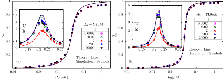
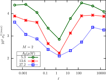
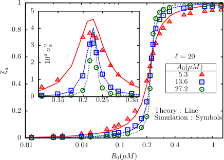
For fixed A0subscript𝐴0A_{0}, the mean active fraction of receptors ΞΎasubscriptπœ‰π‘Ž\xi_{a} undergoes a sharp rise as R0subscript𝑅0R_{0} is increased, as shown in Fig (2). ΞΎasubscriptπœ‰π‘Ž\xi_{a} is independent of β„“β„“\ell, as is clear from the figure, and agrees with the analytical prediction (fixed point). The inset shows the variance in activity, which depends on β„“β„“\ell in a non-monotonic manner (see Fig (3)). In all cases, the maximum of the variance occurs close to the point of the steepest rise in the mean. Note also that for A0=5.3​μsubscript𝐴05.3πœ‡A_{0}=5.3\muM (Fig 2a), the rise is less steeper compared to A0=13.6​μsubscript𝐴013.6πœ‡A_{0}=13.6\muM (Fig 2b); for same β„“β„“\ell, the variance is more in (a), but has a sharper peak in (b). For fixed β„“β„“\ell, and changing A0subscript𝐴0A_{0}, the mean shows the expected ultrasensitive rise as function of R0subscript𝑅0R_{0} (Fig4). For the set of parameters used here in Table 1, the critical value for R0subscript𝑅0R_{0} corresponding to Ξ±=1𝛼1\alpha=1 (29) is R0c=0.224​μsuperscriptsubscript𝑅0𝑐0.224πœ‡R_{0}^{c}=0.224\muM, which agrees with our observations in Fig4. The variance (Fig 4 inset) develops a sharper peak for larger A0subscript𝐴0A_{0}. However, note that, unlike our earlier observations[2] in the GK model (M=1) with only fully inactive and fully active states, the peak value of the variance here does not seem to increase with A0subscript𝐴0A_{0}.

Refer to caption
Figure 2: The mean total active fraction ΞΎΒ―asubscriptΒ―πœ‰π‘Ž\overline{\xi}_{a} versus R0subscript𝑅0R_{0} is independent of β„“β„“\ell; a manifestation of perfect adaptation as predicted by BL model. The figures show the results for two values of A0subscript𝐴0A_{0}, 5.3ΞΌπœ‡\muM (a) and 13.6ΞΌπœ‡\muM (b). In both the figures, the insets show the corresponding variances. Note that the maximum of the variance occurs at the same R0subscript𝑅0R_{0} for various β„“β„“\ell.
Refer to caption
Figure 3: The maximum variance, as determined from simulation data, is plotted against β„“β„“\ell for three different A0subscript𝐴0A_{0}. Interestingly, the maximum is a non-monotonic function of β„“β„“\ell, and appears to have a minimum around β„“=2β„“2\ell=2.
Refer to caption
Figure 4: The mean active fraction of receptors ΞΎΒ―asubscriptΒ―πœ‰π‘Ž\overline{\xi}_{a} plotted against R0subscript𝑅0R_{0} for three different A0subscript𝐴0A_{0} and fixed β„“=20β„“20\ell=20. Inset: The corresponding variances.

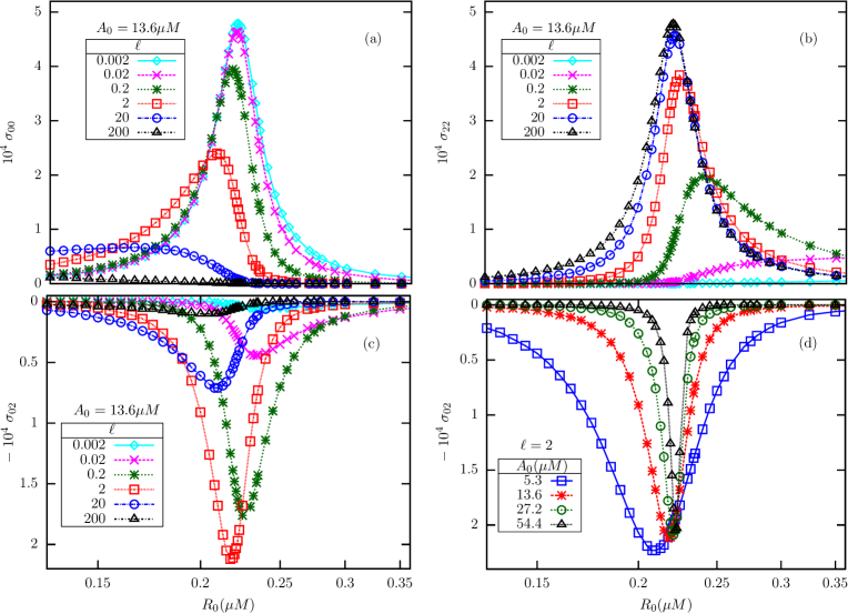
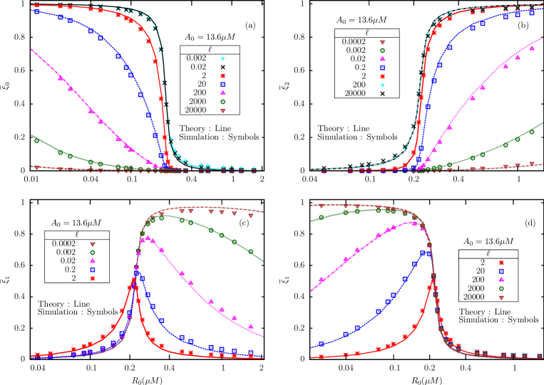
Why would Οƒa2superscriptsubscriptπœŽπ‘Ž2\sigma_{a}^{2} show a non-monotonic variation with β„“β„“\ell? To find out, we studied the mathematical expressions for the individual variances Οƒ00,Οƒ22subscript𝜎00subscript𝜎22\sigma_{00},\sigma_{22} and the covariance Οƒ02subscript𝜎02\sigma_{02} as functions of R0subscript𝑅0R_{0} and β„“β„“\ell, at fixed A0subscript𝐴0A_{0}. The plots, shown in Fig 5, indicate that the non-monotonicity originates from the covariance Οƒ02subscript𝜎02\sigma_{02} between the fully inactive and fully active methylation levels. Both Οƒ00subscript𝜎00\sigma_{00} (Fig 5a) and Οƒ22subscript𝜎22\sigma_{22} (Fig 5b) have their peaks near Rcsubscript𝑅𝑐R_{c}; but while the peak value of Οƒ00subscript𝜎00\sigma_{00} is a decreasing function of β„“β„“\ell, that of Οƒ22subscript𝜎22\sigma_{22} is an increasing function of β„“β„“\ell. Οƒ02subscript𝜎02\sigma_{02} (Fig 5c and d) is negative throughout and has its minimum near Rcsubscript𝑅𝑐R_{c}; however, in (c) the lowest value changes non-monotonically with β„“β„“\ell. From (17), it is seen that Οƒa2superscriptsubscriptπœŽπ‘Ž2\sigma_{a}^{2} is dominated by Οƒ00subscript𝜎00\sigma_{00} for small β„“β„“\ell, while the large β„“β„“\ell behavior is dominated by Οƒ22subscript𝜎22\sigma_{22}. In the intermediate β„“β„“\ell regime, Οƒ02subscript𝜎02\sigma_{02} also contributes significantly, and therefore the non-monotonic variation of its minimum value with β„“β„“\ell affects the peak value of Οƒa2superscriptsubscriptπœŽπ‘Ž2\sigma_{a}^{2}, which appears to be minimized near β„“=2β„“2\ell=2.

Refer to caption
Figure 5: The theoretical plots show the variances Οƒ00subscript𝜎00\sigma_{00}(a), Οƒ22subscript𝜎22\sigma_{22}(b) and the covariance Οƒ02subscript𝜎02\sigma_{02}(c and d). For fixed A0subscript𝐴0A_{0}, near the critical point, Οƒ00subscript𝜎00\sigma_{00} is a decreasing function of β„“β„“\ell, while Οƒ22subscript𝜎22\sigma_{22} is an increasing function of the same. By contrast, the covariance Οƒ02subscript𝜎02\sigma_{02} (c) displays non-monotonic change with β„“β„“\ell near the critical point, with a minimum reached near β„“=2β„“2\ell=2 (compare with Fig 3). But Οƒ02subscript𝜎02\sigma_{02} (d) varies monotonically with A0subscript𝐴0A_{0} for fixed β„“β„“\ell.

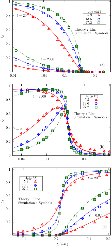
Next, we try to understand how the receptors distribute themselves among different methylation levels and the roles of β„“β„“\ell and A0subscript𝐴0A_{0} in this distribution. For fixed A0subscript𝐴0A_{0} and very small β„“β„“\ell, the fraction of receptors in the lowest methylation level (always inactive) state shows an ultrasensitive transition from near-unity to near-zero across Rcsubscript𝑅𝑐R_{c}. With increase in β„“β„“\ell, the transition becomes less sharper/smoother leading to ΞΎ0subscriptπœ‰0\xi_{0} being almost zero in the entire range of R0subscript𝑅0R_{0} for very large β„“β„“\ell, as given in Fig (6a). On the other hand, the fraction in the highest methylation level (always active) state is almost zero for very small β„“β„“\ell and then increases in the upper-critical regime with increase in β„“β„“\ell, finally leading to an ultrasensitive switch from near-zero to near-unity for very large β„“β„“\ell Fig (6b). But the fraction in the intermediate methylation level exhibits switch-like behaviors of opposite nature at very low and high β„“β„“\ell values; while for intermediate β„“β„“\ell, it shows non-monotonic change with R0subscript𝑅0R_{0} with a peak near Rcsubscript𝑅𝑐R_{c} Fig (6c and d). With increase in A0subscript𝐴0A_{0}, the transitions in ΞΎΒ―0subscriptΒ―πœ‰0\overline{\xi}_{0}, ΞΎΒ―1subscriptΒ―πœ‰1\overline{\xi}_{1} and ΞΎΒ―2subscriptΒ―πœ‰2\overline{\xi}_{2} become sharper (Fig 7), and agrees with the predictions made in (28) and (32). Therefore, in the β„“β†’0β†’β„“0\ell\to 0 as well as β„“β†’βˆžβ†’β„“\ell\to\infty regimes, the system effectively separates into two different GK-like two-state modules, with the population mostly shared between m=0π‘š0m=0 and m=1π‘š1m=1 states in the first case, and between m=1π‘š1m=1 and m=2π‘š2m=2 in the second case.

Refer to caption
Figure 6: The average fractions of receptors in different methylation levels (a) ΞΎΒ―0subscriptΒ―πœ‰0\overline{\xi}_{0} (b) ΞΎΒ―2subscriptΒ―πœ‰2\overline{\xi}_{2} (c) ΞΎΒ―1subscriptΒ―πœ‰1\overline{\xi}_{1} at low ligand concentrations, and (d) ΞΎΒ―1subscriptΒ―πœ‰1\overline{\xi}_{1} at high ligand concentrations, as a function of an internal enzyme concentration (R0subscript𝑅0R_{0}), for fixed substrate concentration A0=13.6​μsubscript𝐴013.6πœ‡A_{0}=13.6\muM.
Refer to caption
Figure 7: A comparison of theoretical and simulation results for the mean fractions of receptors in three states, viz., ΞΎΒ―0subscriptΒ―πœ‰0\overline{\xi}_{0}, ΞΎΒ―1subscriptΒ―πœ‰1\overline{\xi}_{1} and ΞΎΒ―2subscriptΒ―πœ‰2\overline{\xi}_{2} plotted against R0subscript𝑅0R_{0}, for various substrate concentrations A0subscript𝐴0A_{0}, for two different values of β„“β„“\ell (indicated in the figures).

4.2 Simulation results for M>2𝑀2M>2

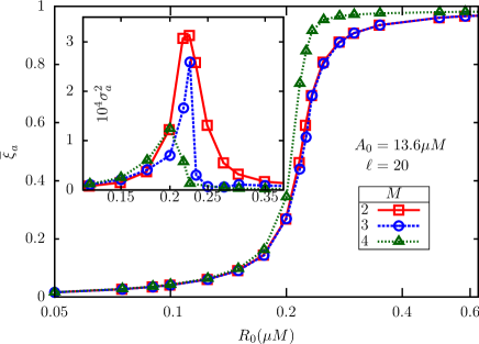
Numerical simulations for models with more intermediate methylation levels, namely M=3𝑀3M=3 and M=4𝑀4M=4 were also carried out for a limited range of values of β„“β„“\ell and A0subscript𝐴0A_{0}. Fig 8 shows a comparison of the mean and variance in active fraction between models with M=2,3𝑀23M=2,3 and 4, for β„“=20β„“20\ell=20 and A0=13.6​μsubscript𝐴013.6πœ‡A_{0}=13.6\muM. For larger M𝑀M, the mean shows sharper rise near R0=Rcsubscript𝑅0subscript𝑅𝑐R_{0}=R_{c}, but the peak value of the variance for M=4𝑀4M=4 is only about a third of the corresponding number for M=2𝑀2M=2. In general, models with larger number of intermediate states has smaller fluctuations in activity, presumably due to the dominant role of inter-state covariances.
Refer to caption
Figure 8: The mean active fractions of receptors in BL models with M=2,3,4𝑀234M=2,3,4 in simulations, with substrate concentration fixed at A0=13.6​μ​Msubscript𝐴013.6πœ‡π‘€A_{0}=13.6\mu M. The attractant concentration is β„“=20β„“20\ell=20. The inset displays the corresponding variances. The numerical results establish that the qualitative behavior of the BL model, in particular, the ZOU transition, remains unchanged in presence of additional intermediate methylation levels.

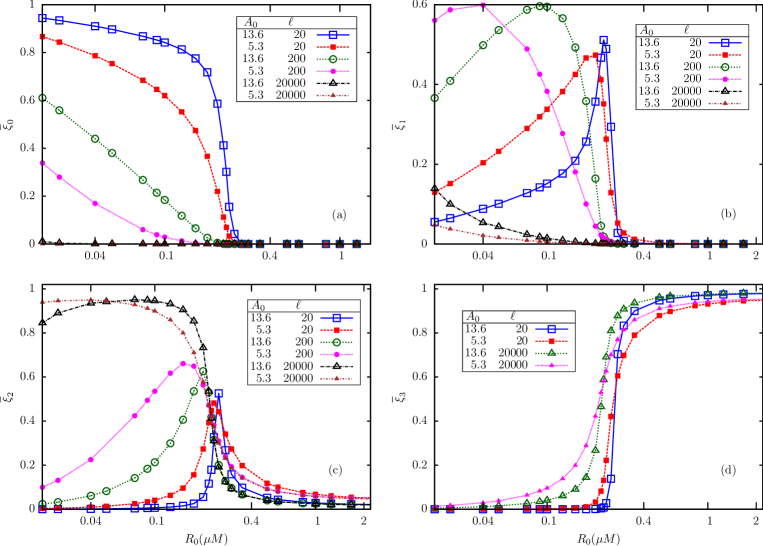
Next, we investigated whether the reduction to two independent two-state models which was found for M=2𝑀2M=2 works well for higher M𝑀M as well. In Fig 9a-d, we show, for M=3𝑀3M=3, the four mean populations ΞΎΒ―0,ΞΎΒ―1,ΞΎΒ―2subscriptΒ―πœ‰0subscriptΒ―πœ‰1subscriptΒ―πœ‰2\overline{\xi}_{0},\overline{\xi}_{1},\overline{\xi}_{2} and ΞΎΒ―3subscriptΒ―πœ‰3\overline{\xi}_{3} respectively for a limited range of β„“β„“\ell and two different values of A0subscript𝐴0A_{0}. Similar to our observations in M=2𝑀2M=2 model, we see that the system effectively reduces to two different 2-state (M=1𝑀1M=1) models. For low β„“β„“\ell (e.g. β„“=20β„“20\ell=20), most of the receptors are in m=0π‘š0m=0 or m=3π‘š3m=3 states; in fact, ΞΎΒ―0subscriptΒ―πœ‰0\overline{\xi}_{0} and ΞΎΒ―3subscriptΒ―πœ‰3\overline{\xi}_{3} show near-ultrasensitive fall and rise respectively across Rcsubscript𝑅𝑐R_{c}. For high β„“β„“\ell (e.g. β„“=20,000β„“20000\ell=20,000), while both ΞΎΒ―0subscriptΒ―πœ‰0\overline{\xi}_{0} and ΞΎΒ―1subscriptΒ―πœ‰1\overline{\xi}_{1} become smaller as A0subscript𝐴0A_{0} is increased, ΞΎΒ―2subscriptΒ―πœ‰2\overline{\xi}_{2} and ΞΎΒ―3subscriptΒ―πœ‰3\overline{\xi}_{3} become dominant; now, ΞΎΒ―2subscriptΒ―πœ‰2\overline{\xi}_{2} falls abruptly as R0subscript𝑅0R_{0} crosses Rcsubscript𝑅𝑐R_{c}, while ΞΎΒ―3subscriptΒ―πœ‰3\overline{\xi}_{3} rises in a similar way. Therefore, for M=3𝑀3M=3 as well, we observe that the system splits into two different GK modules in the limits β„“β†’0β†’β„“0\ell\to 0 and β„“β†’βˆžβ†’β„“\ell\to\infty.

The recent work by Pontius et al. [12] also studied mean and fluctuations in receptor activity in E.coli by varying the enzyme ratio [CheR]/[CheB]. While their model includes more features of chemotaxis receptors like clustering, allosteric interactions and enzyme brachiation, it also suffers from a few drawbacks, in our opinion. (a) In their analytical studies, the total methylation level in a cell is treated as the fundamental stochastic variable, whose dynamics is described by a phenomenological Langevin equation obtained by invoking the LNA; by contrast, our model has the receptor populations in various methylation levels as the basic variables, whose joint probability distribution follows a multivariate LFPE. (b) No direct quantitative comparisons between model predictions and stochastic simulations were done in their paper, while our model predictions are shown to agree well with simulations. (c) Attractant concentration was not included as a parameter in their model, while it is explicitly included in ours, and its effect on the ZOU transition has been explored in detail.
Refer to caption
Figure 9: Simulation results for the mean fractions of receptors in methylation states (a) m=0π‘š0m=0 (b) m=1π‘š1m=1 (c) m=2π‘š2m=2 and (d) m=3π‘š3m=3 in M=3𝑀3M=3 model, for two different substrate concentrations A0=5.3​μsubscript𝐴05.3πœ‡A_{0}=5.3\muM and 13.6ΞΌπœ‡\muM, and a few different values of β„“β„“\ell.

4.3 Change in mean kinase activity in response to a change in attractant concentration

Bacteria perform chemotaxis by responding to time-dependent changes in attractant/repellent concentration in its immediate environment. In this section, we explore the response characteristics of our 3-state model to a time-dependent change in attractant concentration, within linear response theory, applicable to weak perturbations. Let us consider a situation when a time-dependent change δ​L​(t)𝛿𝐿𝑑\delta L(t) in the external ligand concentration is switched on in the extracellular environment of the bacterium at t=0𝑑0t=0, such that L​(t)β†’L+δ​L​(t)→𝐿𝑑𝐿𝛿𝐿𝑑L(t)\to L+\delta L(t) for tβ‰₯0𝑑0t\geq 0, while L​(t)=L𝐿𝑑𝐿L(t)=L for t<0𝑑0t<0. Because ligand binding renders a receptor in the intermediate methylation level inactive, there is a change in the mean net activity at later times, which may be expressed in the general form

δ​ξa¯​(t)=∫0t𝑑t′​χa​(tβˆ’tβ€²)​δ​L​(tβ€²)𝛿¯subscriptπœ‰π‘Žπ‘‘superscriptsubscript0𝑑differential-dsuperscript𝑑′subscriptπœ’π‘Žπ‘‘superscript𝑑′𝛿𝐿superscript𝑑′\delta\overline{\xi_{a}}(t)=\int_{0}^{t}dt^{\prime}\chi_{a}(t-t^{\prime})\delta L(t^{\prime}) (33)

where Ο‡a​(t)subscriptπœ’π‘Žπ‘‘\chi_{a}(t) is the response function for mean receptor activity, which can be computed by submitting the system to a (small) step-like change in ligand concentration; δ​L​(t)=δ​Lsβ€‹Ξ˜β€‹(t)𝛿𝐿𝑑𝛿subscriptπΏπ‘ Ξ˜π‘‘\delta L(t)=\delta L_{s}\Theta(t) where Ξ˜β€‹(t)Ξ˜π‘‘\Theta(t) is the Heaviside theta-function and δ​Ls𝛿subscript𝐿𝑠\delta L_{s} is the size of the step. Let δ​ξaΒ―(step)​(t)𝛿superscriptΒ―subscriptπœ‰π‘Žstep𝑑\delta\overline{\xi_{a}}^{\rm(step)}(t) be the corresponding response. From (33), it follows that

Ο‡a​(t)=1δ​Ls​dd​t​δ​ξ¯a(step)​(t)subscriptπœ’π‘Žπ‘‘1𝛿subscript𝐿𝑠𝑑𝑑𝑑𝛿superscriptsubscriptΒ―πœ‰π‘Žstep𝑑\chi_{a}(t)=\frac{1}{\delta L_{s}}\frac{d}{dt}\delta\overline{\xi}_{a}^{\rm(step)}(t) (34)

From (17), we find

δ​ξ¯a​(t)=βˆ’KLL+KL​δ​ξ¯0​(t)+LL+KL​δ​ξ¯2​(t)βˆ’KL(L+KL)2​(1βˆ’ΞΎ0βˆ—βˆ’ΞΎ2βˆ—)​δ​L​(t),𝛿subscriptΒ―πœ‰π‘Žπ‘‘subscript𝐾𝐿𝐿subscript𝐾𝐿𝛿subscriptΒ―πœ‰0𝑑𝐿𝐿subscript𝐾𝐿𝛿subscriptΒ―πœ‰2𝑑subscript𝐾𝐿superscript𝐿subscript𝐾𝐿21superscriptsubscriptπœ‰0superscriptsubscriptπœ‰2𝛿𝐿𝑑\delta\overline{\xi}_{a}(t)=-\frac{K_{L}}{L+K_{L}}\delta\overline{\xi}_{0}(t)+\frac{L}{L+K_{L}}\delta\overline{\xi}_{2}(t)-\frac{K_{L}}{(L+K_{L})^{2}}(1-\xi_{0}^{*}-\xi_{2}^{*})\delta L(t), (35)

where δ​ξ¯0​(t)𝛿subscriptΒ―πœ‰0𝑑\delta\overline{\xi}_{0}(t) and δ​ξ¯2​(t)𝛿subscriptΒ―πœ‰2𝑑\delta\overline{\xi}_{2}(t) are the changes in ΞΎΒ―0subscriptΒ―πœ‰0\overline{\xi}_{0} and ΞΎΒ―2subscriptΒ―πœ‰2\overline{\xi}_{2}, respectively, in response to a change δ​L​(t)𝛿𝐿𝑑\delta L(t) in the ligand concentration, and are evaluated using (6). The resulting equations have the form

dd​t​δ​ξ¯m=βˆ‘n=0,2Ξ²m​n​δ​ξ¯n​(t)+Ξ³m​δ​L​(t)​m=0,2formulae-sequence𝑑𝑑𝑑𝛿subscriptΒ―πœ‰π‘šsubscript𝑛02subscriptπ›½π‘šπ‘›π›ΏsubscriptΒ―πœ‰π‘›π‘‘subscriptπ›Ύπ‘šπ›ΏπΏπ‘‘π‘š02\frac{d}{dt}\delta\overline{\xi}_{m}=\sum_{n=0,2}\beta_{mn}\delta\overline{\xi}_{n}(t)+\gamma_{m}\delta L(t)~{}~{}~{}m=0,2 (36)

where the coefficients Ξ²m​nsubscriptπ›½π‘šπ‘›\beta_{mn} have been defined earlier, following (10), while Ξ³m=βˆ‚vm/βˆ‚L|πƒβˆ—subscriptπ›Ύπ‘ševaluated-atsubscriptπ‘£π‘šπΏsuperscript𝝃\gamma_{m}=\partial v_{m}/\partial L|_{\boldsymbol{\xi}^{*}}. Explicit expressions for both Ξ²m​nsubscriptπ›½π‘šπ‘›\beta_{mn} and Ξ³msubscriptπ›Ύπ‘š\gamma_{m} are given in 6.2.

It is convenient to subject (35) and (36) to Laplace transforms, after putting δ​L​(t)=δ​Lsβ€‹Ξ˜β€‹(t)𝛿𝐿𝑑𝛿subscriptπΏπ‘ Ξ˜π‘‘\delta L(t)=\delta L_{s}\Theta(t), and use (34) to compute the response function. For the Laplace transform of Ο‡a​(t)subscriptπœ’π‘Žπ‘‘\chi_{a}(t), we find

Ο‡~a​(s)=βˆ’KLL+KL​χ~0​(s)+LL+KL​χ~2​(s)βˆ’KL(L+KL)2​(1βˆ’ΞΎ0βˆ—βˆ’ΞΎ2βˆ—)subscript~πœ’π‘Žπ‘ subscript𝐾𝐿𝐿subscript𝐾𝐿subscript~πœ’0𝑠𝐿𝐿subscript𝐾𝐿subscript~πœ’2𝑠subscript𝐾𝐿superscript𝐿subscript𝐾𝐿21superscriptsubscriptπœ‰0superscriptsubscriptπœ‰2\tilde{\chi}_{a}(s)=-\frac{K_{L}}{L+K_{L}}\tilde{\chi}_{{}_{0}}(s)+\frac{L}{L+K_{L}}\tilde{\chi}_{{}_{2}}(s)-\frac{K_{L}}{(L+K_{L})^{2}}(1-\xi_{0}^{*}-\xi_{2}^{*}) (37)

where Ο‡~m​(s)subscript~πœ’π‘šπ‘ \tilde{\chi}_{m}(s) are Laplace transforms of Ο‡m​(t)subscriptπœ’π‘šπ‘‘\chi_{m}(t) (m=0,2π‘š02m=0,2) which are defined through the relations δ​ξ¯m​(t)=∫0tΟ‡m​(tβˆ’tβ€²)​δ​L​(tβ€²)​𝑑t′𝛿subscriptΒ―πœ‰π‘šπ‘‘superscriptsubscript0𝑑subscriptπœ’π‘šπ‘‘superscript𝑑′𝛿𝐿superscript𝑑′differential-dsuperscript𝑑′\delta\overline{\xi}_{m}(t)=\int_{0}^{t}\chi_{m}(t-t^{\prime})\delta L(t^{\prime})dt^{\prime}. The explicit expressions turn out to be

Ο‡~0​(s)subscript~πœ’0𝑠\displaystyle\tilde{\chi}_{{}_{0}}(s) =\displaystyle= [(sβˆ’Ξ²22)​γ0+Ξ²02​γ2]/ddelimited-[]𝑠subscript𝛽22subscript𝛾0subscript𝛽02subscript𝛾2𝑑\displaystyle[(s-\beta_{22})\gamma_{0}+\beta_{02}\gamma_{2}]/d
Ο‡~2​(s)subscript~πœ’2𝑠\displaystyle\tilde{\chi}_{{}_{2}}(s) =\displaystyle= [Ξ²20​γ0+(sβˆ’Ξ²00)​γ2]/d,delimited-[]subscript𝛽20subscript𝛾0𝑠subscript𝛽00subscript𝛾2𝑑\displaystyle[\beta_{20}\gamma_{0}+(s-\beta_{00})\gamma_{2}]/d, (38)

where d=(sβˆ’Ξ²00)​(sβˆ’Ξ²22)βˆ’Ξ²02​β20𝑑𝑠subscript𝛽00𝑠subscript𝛽22subscript𝛽02subscript𝛽20d=(s-\beta_{00})(s-\beta_{22})-\beta_{02}\beta_{20}. We have confirmed that the response function curve computed in (37) encloses zero area, i.e., Ο‡~a​(0)=0subscript~πœ’π‘Ž00\tilde{\chi}_{a}(0)=0, which is a manifestation of the perfect adaptation (regaining the pre-stimulus state within few seconds) property of the bacterium, reproduced in the BL model (in our notation, this property implies lack of dependence of ΞΎΒ―asubscriptΒ―πœ‰π‘Ž\overline{\xi}_{a} on β„“β„“\ell in steady state, recall Fig (2)). In 6.3, we use the results in (37) and (4.3) to derive the chemotactic response function, which determines the fractional change in clockwise bias of the flagellar motor in response to temporal variations in attractant concentration, and consequently the chemotactic drift.

5 Discussion

The subject of the present study is the BL model of conformational dynamics of chemotaxis receptors in Escherichia coli. According to this model, a receptor undergoes stochastic switching between its active and inactive states, depending on its level of methylation and ligandation. The methylation and demethylation of receptors is carried out by two enzymes, viz. methyltransferase CheR and methylesterase CheB, acting antagonistically; the overall structure of the circuit is similar to the two-state (e.g. active/inactive) covalent modification scheme studied originally by GK [1]. This system is characterized by ZOU, a switch-like transition between all-inactive to all-active phases, in the limit of infinitely large substrate concentration. In the present paper, we investigated ZOU in the BL model within a stochastic formulation where the number N𝑁N of receptors is treated finite. For analytical tractability, we first study a model with a single intermediate partially active state sandwiched between the fully inactive and fully active states. We show rigorously that the mean activity shows ultrasensitive response to increase in [CheR] (at fixed [CheB]) in the limit Nβ†’βˆžβ†’π‘N\to\infty, independent of the attractant concentration L𝐿L. At the same time, its variance Οƒa2superscriptsubscriptπœŽπ‘Ž2\sigma_{a}^{2} is a non-monotonic function of [CheR] and L𝐿L, as deduced from linear-noise approximation (LNA) and confirmed in numerical simulations. Interestingly, for very low and very high L𝐿L, the system effectively reduces to two different β€œtwo-state” modules, akin to GK switches. The analysis is extended to models with more intermediate methylation levels (E.coli receptor has 3) via numerical simulations. By and large, qualitatively similar behavior is found in all the cases. For E.coli parameters, we find that Οƒa≃10βˆ’2similar-to-or-equalssubscriptπœŽπ‘Žsuperscript102\sigma_{a}\simeq 10^{-2} in the vicinity of the critical point of ZOU, for a large range of L𝐿L, spanning almost 8 orders of magnitude. This estimate agrees with another recent computational study where explicit receptor clustering was included, and receptor activation-inactivation dynamics was stimulated using an equilibrium MWC model [12]. In 6.3, we show that this is also consistent with experimental measurements of [CheYp] fluctuations.

Biochemical noise is likely to be a crucial factor in the motility of E.coli for the following reason. The transition from run to tumble mode of a flagellar motor in E.coli is brought about by a switch in its direction of rotation, from counter-clockwise (CCW) to clockwise (CW). The latter switching is known to occur in an ultrasensitive fashion as a function of [CheYp], the concentration of phosphorylated CheY, which is the response regulator cytoplasmic protein (the phosphorylation being done by active receptors). The ultrasensitive response of flagellar motor for the CW bias with the variation in the concentration of CheYp, was first reported by Cluzel et al. [17] by performing in vivo experiments in single cells in absence of stimulant (attractant/repellent). The authors observed cell to cell variability in the amount of CheYp which was distributed around a mean value (ranging from 0.80.80.8 to 6​μ​M6πœ‡π‘€6\mu M) even for a given concentration of the inducer isopropyl β𝛽\beta-D-thiogalactoside, in short IPTG (used to express CHEY-GFP in PS2001 E. coli strain). CW bias in various cells, pre-induced with different inducer levels, collapsed onto a single sigmoid curve when plotted against CheYp. The measured CW bias in the range 0.10.10.1 to 0.90.90.9 could be fitted to a Hill plot with Hill coefficient H∼10.3Β±1.1similar-to𝐻plus-or-minus10.31.1H\sim 10.3\pm 1.1, with the sensitive part being less than 3​μ3πœ‡3\muM in width. The ability of the cell to execute runs and tumbles in succession depends on placing the intracellular [CheYp] somewhat precisely in this window.

Cluzel et al. proposed that an additional molecular mechanism such as CheZ acting as the [CheYp] regulator can help in retaining the concentration of the latter in the narrow sensitive window of operation. Later, Yuan et al. [24] found from their experiments with cheRcheB cells that the flagellar motor can partially adapt to changes in [CheYp] over a time scale of several minutes, and thereby laterally shift its operating range by about 0.5ΞΌπœ‡\muM. Any likelihood of partial adaptation due to dynamic localization of CheZ (suggested by Lipkow [25]) was ruled out by working with cheRcheBcheZ cells and explicitly showing similar results in both the cases. In 2013, Yuan and Berg [16] carried out a new set of experiments with pre-adapted motors, which showed that the response curve in this case is much steeper, compared to adapted motors (as in [17]) with Hill coefficients ∼16.5Β±1.1similar-toabsentplus-or-minus16.51.1\sim 16.5\pm 1.1 and 20.7Β±1.6plus-or-minus20.71.620.7\pm 1.6 for CW biases of 0.8Β±0.1plus-or-minus0.80.10.8\pm 0.1 and 0.5Β±0.1plus-or-minus0.50.10.5\pm 0.1 respectively. Because of the higher Hill coefficient, the sensitive window of [CheYp] is reduced to about 1ΞΌπœ‡\muM in this case, with center around 3ΞΌπœ‡\muM.

What is the impact of receptor-level noise on the clockwise bias of a single cell ? It is clear that spontaneous fluctuations in receptor activity will produce corresponding changes in [CheYp], which would, in turn, affect the CW bias of the motor(s). In 6.4 we estimate that the maximum standard deviation in clockwise bias (arising from spontaneous fluctuations in [CheYp]) δ​PC​W𝛿subscriptπ‘ƒπΆπ‘Š\delta P_{CW} lies in the range 0.15-0.36 for Hill coefficient H=20𝐻20H=20 [16], with the lower value corresponding to mean CW bias ∼similar-to\sim 0.5 and the upper value for mean CW bias ∼similar-to\sim 0.1. It therefore appears that intrinsic noise could rescue a cell with mean [CheYp] outside the optimal range from being forced to ”run forever” without tumbling. The motor-level adaptation modifies these estimates a little, but our detailed analysis presented in 6.5 shows that this effect is negligible when [CheYp] lies in the range 2.5​μ​Mβˆ’4​μ​M2.5πœ‡π‘€4πœ‡π‘€2.5\mu M-4\mu M, which more than covers the sensitive window. Outside this range, motor-level adaptation increases the standard deviation in CW bias, (see figure in 6.5). We conclude, therefore, that intrinsic noise plays an important role in the run and tumble behavior of E.coli, and by extension, in chemotactic drift as well. A detailed analysis of the latter is presently being carried out and will be reported in the near future.

Being a study focused primarily on exploring the occurrence of ZOU in the BL model, we have not included all the features of signal transduction in E.coli here, even at the level of receptor dynamics. In particular, clustering of receptors and allosteric interactions among them have not been included here, but have been studied recently by other authors[12, 26, 27]. In [12], the authors show via numerical simulations that receptor clustering and enzyme localization make the mean activity a less sensitive function of [CheR], and thus makes the network robust to variations in protein numbers. At the same time, enzyme localization also leads to larger fluctuations in activity, with almost 10-fold increase in variance. Intrinsic biochemical noise arising from spontaneous fluctuations in receptor activity has been shown to be important in explaining the kinetics of flagellar motor-switching[28, 29]. Using a set of parameters extracted from the literature, we show in 6.3 that the variance in activity measured in our simulations (as well as predicted using LNA) appear to be sufficiently large in magnitude to generate the [CheYp] fluctuations observed in experiments[28]. It is therefore likely that receptor clustering and enzyme localization may not be necessary to enhance the noise levels, although it could be important in other aspects of signaling, e.g. signal amplification.

6 Appendices

6.1 Intra and inter-module dynamics in the 3-state receptor-level biochemical reactions

To evaluate the number of receptors in each of the configurations, we employ sQSSA. The essence of sQSSA lies in the assumption that all the modules are weakly coupled (Ξ½rsubscriptπœˆπ‘Ÿ\nu_{r} and Ξ½bsubscriptπœˆπ‘\nu_{b} assumed to be very small compared to other rates involved in the system) and hence detailed balance exists within each module. Under this condition, the mean numbers of intermediate complexes can be expressed in terms of their unbound counterparts as

x~0Β―=RfKr​x0Β―;x~1iΒ―=RfKr​x1iΒ―;x~1aΒ―=BfKb​x1aΒ―;x~2Β―=BfKb​x2Β―;x1iΒ―=LKL​x1aΒ―.formulae-sequenceΒ―subscript~π‘₯0subscript𝑅𝑓subscriptπΎπ‘ŸΒ―subscriptπ‘₯0formulae-sequenceΒ―superscriptsubscript~π‘₯1𝑖subscript𝑅𝑓subscriptπΎπ‘ŸΒ―superscriptsubscriptπ‘₯1𝑖formulae-sequenceΒ―superscriptsubscript~π‘₯1π‘Žsubscript𝐡𝑓subscript𝐾𝑏¯superscriptsubscriptπ‘₯1π‘Žformulae-sequenceΒ―subscript~π‘₯2subscript𝐡𝑓subscript𝐾𝑏¯subscriptπ‘₯2Β―superscriptsubscriptπ‘₯1𝑖𝐿subscript𝐾𝐿¯superscriptsubscriptπ‘₯1π‘Ž\overline{\tilde{x}_{0}}=\frac{R_{f}}{K_{r}}\overline{x_{0}}~{}~{};~{}~{}\overline{\tilde{x}_{1}^{i}}=\frac{R_{f}}{K_{r}}\overline{x_{1}^{i}}~{}~{};~{}~{}\overline{\tilde{x}_{1}^{a}}=\frac{B_{f}}{K_{b}}\overline{x_{1}^{a}}~{}~{};~{}~{}\overline{\tilde{x}_{2}}=\frac{B_{f}}{K_{b}}\overline{x_{2}}~{};~{}~{}\overline{x_{1}^{i}}=\frac{L}{K_{L}}\overline{x_{1}^{a}}. (39)

where Rfsubscript𝑅𝑓R_{f} and Bfsubscript𝐡𝑓B_{f} are the mean concentrations of free/unbound R and B enzymes respectively. After using the module-wise normalization conditions x0+x~0=ΞΎ0subscriptπ‘₯0subscript~π‘₯0subscriptπœ‰0x_{0}+\tilde{x}_{0}=\xi_{0}, x1i+x~1i=ΞΎ1isuperscriptsubscriptπ‘₯1𝑖superscriptsubscript~π‘₯1𝑖superscriptsubscriptπœ‰1𝑖x_{1}^{i}+\tilde{x}_{1}^{i}=\xi_{1}^{i}, x1a+x~1a=ΞΎ1asuperscriptsubscriptπ‘₯1π‘Žsuperscriptsubscript~π‘₯1π‘Žsuperscriptsubscriptπœ‰1π‘Žx_{1}^{a}+\tilde{x}_{1}^{a}=\xi_{1}^{a} and x2+x~2=ΞΎ2subscriptπ‘₯2subscript~π‘₯2subscriptπœ‰2x_{2}+\tilde{x}_{2}=\xi_{2}, we find

x~0¯​(𝝃)Β―subscript~π‘₯0𝝃\displaystyle\overline{\tilde{x}_{0}}(\boldsymbol{\xi}) =\displaystyle= RfRf+Kr​ξ0subscript𝑅𝑓subscript𝑅𝑓subscriptπΎπ‘Ÿsubscriptπœ‰0\displaystyle\frac{R_{f}}{R_{f}+K_{r}}\xi_{0}
x~1i¯​(𝝃)Β―superscriptsubscript~π‘₯1𝑖𝝃\displaystyle\overline{\tilde{x}_{1}^{i}}(\boldsymbol{\xi}) =\displaystyle= RfRf+Kr​ξ1iΒ―subscript𝑅𝑓subscript𝑅𝑓subscriptπΎπ‘ŸΒ―superscriptsubscriptπœ‰1𝑖\displaystyle\frac{R_{f}}{R_{f}+K_{r}}\overline{\xi_{1}^{i}}
x~1a¯​(𝝃)Β―superscriptsubscript~π‘₯1π‘Žπƒ\displaystyle\overline{\tilde{x}_{1}^{a}}(\boldsymbol{\xi}) =\displaystyle= BfBf+Kb​ξ1aΒ―subscript𝐡𝑓subscript𝐡𝑓subscript𝐾𝑏¯superscriptsubscriptπœ‰1π‘Ž\displaystyle\frac{B_{f}}{B_{f}+K_{b}}\overline{\xi_{1}^{a}}
x~2¯​(𝝃)Β―subscript~π‘₯2𝝃\displaystyle\overline{\tilde{x}_{2}}(\boldsymbol{\xi}) =\displaystyle= BfBf+Kb​ξ2subscript𝐡𝑓subscript𝐡𝑓subscript𝐾𝑏subscriptπœ‰2\displaystyle\frac{B_{f}}{B_{f}+K_{b}}\xi_{2}
ΞΎ1iΒ―Β―superscriptsubscriptπœ‰1𝑖\displaystyle\overline{\xi_{1}^{i}} =\displaystyle= LKL​ξ1aΒ―.𝐿subscript𝐾𝐿¯superscriptsubscriptπœ‰1π‘Ž\displaystyle\frac{L}{K_{L}}\overline{\xi_{1}^{a}}. (40)

In the last equation, we have used the assumption of infinitely fast ligand binding and dissociation kinetics. Inter-module equilibrium is expressed through the following flux-balance relations which determine the fixed point πƒβˆ—superscript𝝃\boldsymbol{\xi}^{*}:

Ξ½r​x~0¯​(πƒβˆ—)βˆ’Ξ½b​x~1a¯​(πƒβˆ—)=0=Ξ½r​x~1i¯​(πƒβˆ—)βˆ’Ξ½b​x~2¯​(πƒβˆ—).subscriptπœˆπ‘ŸΒ―subscript~π‘₯0superscript𝝃subscriptπœˆπ‘Β―superscriptsubscript~π‘₯1π‘Žsuperscript𝝃0subscriptπœˆπ‘ŸΒ―superscriptsubscript~π‘₯1𝑖superscript𝝃subscriptπœˆπ‘Β―subscript~π‘₯2superscript𝝃\nu_{r}\overline{\tilde{x}_{0}}(\boldsymbol{\xi^{*}})-\nu_{b}\overline{\tilde{x}_{1}^{a}}(\boldsymbol{\xi}^{*})=0=\nu_{r}\overline{\tilde{x}_{1}^{i}}(\boldsymbol{\xi}^{*})-\nu_{b}\overline{\tilde{x}_{2}}(\boldsymbol{\xi}^{*}). (41)

The free enzyme concentrations Rfsubscript𝑅𝑓R_{f} and Bfsubscript𝐡𝑓B_{f} are determined by the normalization conditions

Rf​(𝝃)+A0​[x0~Β―+x~1iΒ―]=R0subscript𝑅𝑓𝝃subscript𝐴0delimited-[]Β―~subscriptπ‘₯0Β―superscriptsubscript~π‘₯1𝑖subscript𝑅0\displaystyle R_{f}(\boldsymbol{\xi})+A_{0}[\overline{\tilde{x_{0}}}+\overline{\tilde{x}_{1}^{i}}]=R_{0}
Bf​(𝝃)+A0​[x2~Β―+x~1aΒ―]=B0subscript𝐡𝑓𝝃subscript𝐴0delimited-[]Β―~subscriptπ‘₯2Β―superscriptsubscript~π‘₯1π‘Žsubscript𝐡0\displaystyle B_{f}(\boldsymbol{\xi})+A_{0}[\overline{\tilde{x_{2}}}+\overline{\tilde{x}_{1}^{a}}]=B_{0} (42)

Using (6.1) in (6.1) leads to (2.2).

Perfect adaptation (insensitivity of average activity to L):

Although the fixed point πƒβˆ—superscript𝝃\boldsymbol{\xi}^{*} depends on L𝐿L, the mean total active fraction does not; this can be easily shown as follows. The equations (41) for intermodule dynamics, after summing the left hand side give

Ξ½r​(x~0Β―+x~1iΒ―)=Ξ½b​(x~1aΒ―+x~2Β―)subscriptπœˆπ‘ŸΒ―subscript~π‘₯0Β―superscriptsubscript~π‘₯1𝑖subscriptπœˆπ‘Β―superscriptsubscript~π‘₯1π‘ŽΒ―subscript~π‘₯2\nu_{r}(\overline{\tilde{x}_{0}}+\overline{\tilde{x}_{1}^{i}})=\nu_{b}(\overline{\tilde{x}_{1}^{a}}+\overline{\tilde{x}_{2}}) (43)

After substituting the equations for intra-module dynamics (6.1) (in the limit Rfβ‰ͺKrmuch-less-thansubscript𝑅𝑓subscriptπΎπ‘ŸR_{f}\ll K_{r}, Bfβ‰ͺKbmuch-less-thansubscript𝐡𝑓subscript𝐾𝑏B_{f}\ll K_{b}) and the expression for ΞΎasubscriptπœ‰π‘Ž\xi_{a} in terms of ΞΎmsubscriptπœ‰π‘š\xi_{m} (17) in (43), the following quadratic equation for ΞΎaβˆ—superscriptsubscriptπœ‰π‘Ž\xi_{a}^{*}, independent of L𝐿L, is obtained:

ΞΎaβˆ—2​(Ξ½b​B0βˆ’Ξ½r​R0)+ΞΎaβˆ—β€‹[Ξ½r​R0​(A0βˆ’Kb)βˆ’Ξ½b​B0​(Kr+A0)]+Ξ½r​R0​A0​Kb=0.superscriptsubscriptπœ‰π‘Žabsent2subscriptπœˆπ‘subscript𝐡0subscriptπœˆπ‘Ÿsubscript𝑅0superscriptsubscriptπœ‰π‘Ždelimited-[]subscriptπœˆπ‘Ÿsubscript𝑅0subscript𝐴0subscript𝐾𝑏subscriptπœˆπ‘subscript𝐡0subscriptπΎπ‘Ÿsubscript𝐴0subscriptπœˆπ‘Ÿsubscript𝑅0subscript𝐴0subscript𝐾𝑏0\xi_{a}^{*2}(\nu_{b}B_{0}-\nu_{r}R_{0})+\xi_{a}^{*}[\nu_{r}R_{0}(A_{0}-K_{b})-\nu_{b}B_{0}(K_{r}+A_{0})]+\nu_{r}R_{0}A_{0}K_{b}=0. (44)

The solution to the above equation is

ΞΎaβˆ—superscriptsubscriptπœ‰π‘Ž\displaystyle\xi_{a}^{*} =\displaystyle= Ξ½b​B0​(A0+Kr)βˆ’Ξ½r​R0​(A0βˆ’Kb)2​(Ξ½b​B0βˆ’Ξ½r​R0)subscriptπœˆπ‘subscript𝐡0subscript𝐴0subscriptπΎπ‘Ÿsubscriptπœˆπ‘Ÿsubscript𝑅0subscript𝐴0subscript𝐾𝑏2subscriptπœˆπ‘subscript𝐡0subscriptπœˆπ‘Ÿsubscript𝑅0\displaystyle\frac{\nu_{b}B_{0}(A_{0}+K_{r})-\nu_{r}R_{0}(A_{0}-K_{b})}{2(\nu_{b}B_{0}-\nu_{r}R_{0})} (45)
+\displaystyle+ [Ξ½b​B0​(A0+Kr)βˆ’Ξ½r​R0​(A0βˆ’Kb)]2βˆ’4​νr​R0​A0​Kb​(Ξ½b​B0βˆ’Ξ½r​R0)2​(Ξ½b​B0βˆ’Ξ½r​R0)superscriptdelimited-[]subscriptπœˆπ‘subscript𝐡0subscript𝐴0subscriptπΎπ‘Ÿsubscriptπœˆπ‘Ÿsubscript𝑅0subscript𝐴0subscript𝐾𝑏24subscriptπœˆπ‘Ÿsubscript𝑅0subscript𝐴0subscript𝐾𝑏subscriptπœˆπ‘subscript𝐡0subscriptπœˆπ‘Ÿsubscript𝑅02subscriptπœˆπ‘subscript𝐡0subscriptπœˆπ‘Ÿsubscript𝑅0\displaystyle\frac{\sqrt{[\nu_{b}B_{0}(A_{0}+K_{r})-\nu_{r}R_{0}(A_{0}-K_{b})]^{2}-4\nu_{r}R_{0}A_{0}K_{b}(\nu_{b}B_{0}-\nu_{r}R_{0})}}{2(\nu_{b}B_{0}-\nu_{r}R_{0})}

6.2 Evaluation of various parameters

The expressions of Ξ²m​nsubscriptπ›½π‘šπ‘›\beta_{mn} can be obtained by differentiating (2.2). Note that the expressions for vmsubscriptπ‘£π‘šv_{m} contain Rfsubscript𝑅𝑓R_{f} and Bfsubscript𝐡𝑓B_{f} which are in turn functions of ΞΎmsubscriptπœ‰π‘š\xi_{m}. Therefore,

Ξ²m​n=(βˆ‚vmβˆ‚ΞΎn+βˆ‚vmβˆ‚Rfβ€‹βˆ‚Rfβˆ‚ΞΎn+βˆ‚vmβˆ‚Bfβ€‹βˆ‚Bfβˆ‚ΞΎn)πƒβˆ—,subscriptπ›½π‘šπ‘›subscriptsubscriptπ‘£π‘šsubscriptπœ‰π‘›subscriptπ‘£π‘šsubscript𝑅𝑓subscript𝑅𝑓subscriptπœ‰π‘›subscriptπ‘£π‘šsubscript𝐡𝑓subscript𝐡𝑓subscriptπœ‰π‘›superscript𝝃\beta_{mn}=\Bigg{(}\frac{\partial v_{m}}{\partial\xi_{n}}+\frac{\partial v_{m}}{\partial R_{f}}\frac{\partial R_{f}}{\partial\xi_{n}}+\frac{\partial v_{m}}{\partial B_{f}}\frac{\partial B_{f}}{\partial\xi_{n}}\Bigg{)}_{\boldsymbol{\xi^{*}}}, (46)

where

βˆ‚v0βˆ‚ΞΎ0subscript𝑣0subscriptπœ‰0\displaystyle\frac{\partial v_{0}}{\partial\xi_{0}} =\displaystyle= βˆ’(Ξ½b​BfKb​KLL+KL+Ξ½r​RfKr)subscriptπœˆπ‘subscript𝐡𝑓subscript𝐾𝑏subscript𝐾𝐿𝐿subscript𝐾𝐿subscriptπœˆπ‘Ÿsubscript𝑅𝑓subscriptπΎπ‘Ÿ\displaystyle-\Big{(}\frac{\nu_{b}B_{f}}{K_{b}}\frac{K_{L}}{L+K_{L}}+\frac{\nu_{r}R_{f}}{K_{r}}\Big{)}
βˆ‚v0βˆ‚ΞΎ2subscript𝑣0subscriptπœ‰2\displaystyle\frac{\partial v_{0}}{\partial\xi_{2}} =\displaystyle= βˆ’Ξ½b​BfKb​KLL+KLsubscriptπœˆπ‘subscript𝐡𝑓subscript𝐾𝑏subscript𝐾𝐿𝐿subscript𝐾𝐿\displaystyle-\frac{\nu_{b}B_{f}}{K_{b}}\frac{K_{L}}{L+K_{L}}
βˆ‚v2βˆ‚ΞΎ0subscript𝑣2subscriptπœ‰0\displaystyle\frac{\partial v_{2}}{\partial\xi_{0}} =\displaystyle= βˆ’Ξ½r​RfKr​LL+KLsubscriptπœˆπ‘Ÿsubscript𝑅𝑓subscriptπΎπ‘ŸπΏπΏsubscript𝐾𝐿\displaystyle-\frac{\nu_{r}R_{f}}{K_{r}}\frac{L}{L+K_{L}}
βˆ‚v2βˆ‚ΞΎ2subscript𝑣2subscriptπœ‰2\displaystyle\frac{\partial v_{2}}{\partial\xi_{2}} =\displaystyle= βˆ’(Ξ½r​RfKr​LL+KL+Ξ½b​BfKb)subscriptπœˆπ‘Ÿsubscript𝑅𝑓subscriptπΎπ‘ŸπΏπΏsubscript𝐾𝐿subscriptπœˆπ‘subscript𝐡𝑓subscript𝐾𝑏\displaystyle-\Big{(}\frac{\nu_{r}R_{f}}{K_{r}}\frac{L}{L+K_{L}}+\frac{\nu_{b}B_{f}}{K_{b}}\Big{)}
βˆ‚v0βˆ‚Rfsubscript𝑣0subscript𝑅𝑓\displaystyle\frac{\partial v_{0}}{\partial R_{f}} =\displaystyle= βˆ’Ξ½rKr​ξ0subscriptπœˆπ‘ŸsubscriptπΎπ‘Ÿsubscriptπœ‰0\displaystyle-\frac{\nu_{r}}{K_{r}}\xi_{0}
βˆ‚v0βˆ‚Bfsubscript𝑣0subscript𝐡𝑓\displaystyle\frac{\partial v_{0}}{\partial B_{f}} =\displaystyle= Ξ½bKb​KLL+KL​(1βˆ’ΞΎ0βˆ’ΞΎ2)subscriptπœˆπ‘subscript𝐾𝑏subscript𝐾𝐿𝐿subscript𝐾𝐿1subscriptπœ‰0subscriptπœ‰2\displaystyle\frac{\nu_{b}}{K_{b}}\frac{K_{L}}{L+K_{L}}(1-\xi_{0}-\xi_{2})
βˆ‚v2βˆ‚Rfsubscript𝑣2subscript𝑅𝑓\displaystyle\frac{\partial v_{2}}{\partial R_{f}} =\displaystyle= Ξ½rKr​LL+KL​(1βˆ’ΞΎ0βˆ’ΞΎ2)subscriptπœˆπ‘ŸsubscriptπΎπ‘ŸπΏπΏsubscript𝐾𝐿1subscriptπœ‰0subscriptπœ‰2\displaystyle\frac{\nu_{r}}{K_{r}}\frac{L}{L+K_{L}}(1-\xi_{0}-\xi_{2})
βˆ‚v2βˆ‚Bfsubscript𝑣2subscript𝐡𝑓\displaystyle\frac{\partial v_{2}}{\partial B_{f}} =\displaystyle= βˆ’Ξ½bKb​ξ2βˆ—subscriptπœˆπ‘subscript𝐾𝑏superscriptsubscriptπœ‰2\displaystyle-\frac{\nu_{b}}{K_{b}}\xi_{2}^{*} (48)
βˆ‚Rfβˆ‚ΞΎ0subscript𝑅𝑓subscriptπœ‰0\displaystyle\frac{\partial R_{f}}{\partial\xi_{0}} =\displaystyle= βˆ’R0​Kr​(L+KL)​A0​KL[Kr​(L+KL)+A0​(KL​ξ0+L​(1βˆ’ΞΎ2))]2subscript𝑅0subscriptπΎπ‘ŸπΏsubscript𝐾𝐿subscript𝐴0subscript𝐾𝐿superscriptdelimited-[]subscriptπΎπ‘ŸπΏsubscript𝐾𝐿subscript𝐴0subscript𝐾𝐿subscriptπœ‰0𝐿1subscriptπœ‰22\displaystyle-\frac{R_{0}K_{r}(L+K_{L})A_{0}K_{L}}{\Big{[}K_{r}(L+K_{L})+A_{0}\big{(}K_{L}\xi_{0}+L(1-\xi_{2})\big{)}\Big{]}^{2}}
βˆ‚Rfβˆ‚ΞΎ2subscript𝑅𝑓subscriptπœ‰2\displaystyle\frac{\partial R_{f}}{\partial\xi_{2}} =\displaystyle= R0​Kr​(L+KL)​A0​L[Kr​(L+KL)+A0​(KL​ξ0+L​(1βˆ’ΞΎ2))]2subscript𝑅0subscriptπΎπ‘ŸπΏsubscript𝐾𝐿subscript𝐴0𝐿superscriptdelimited-[]subscriptπΎπ‘ŸπΏsubscript𝐾𝐿subscript𝐴0subscript𝐾𝐿subscriptπœ‰0𝐿1subscriptπœ‰22\displaystyle\frac{R_{0}K_{r}(L+K_{L})A_{0}L}{\Big{[}K_{r}(L+K_{L})+A_{0}\big{(}K_{L}\xi_{0}+L(1-\xi_{2})\big{)}\Big{]}^{2}}
βˆ‚Bfβˆ‚ΞΎ0subscript𝐡𝑓subscriptπœ‰0\displaystyle\frac{\partial B_{f}}{\partial\xi_{0}} =\displaystyle= B0​Kb​(L+KL)​A0​KL[Kb​(L+KL)+A0​(KL​(1βˆ’ΞΎ0)+L​ξ2)]2subscript𝐡0subscript𝐾𝑏𝐿subscript𝐾𝐿subscript𝐴0subscript𝐾𝐿superscriptdelimited-[]subscript𝐾𝑏𝐿subscript𝐾𝐿subscript𝐴0subscript𝐾𝐿1subscriptπœ‰0𝐿subscriptπœ‰22\displaystyle\frac{B_{0}K_{b}(L+K_{L})A_{0}K_{L}}{\Big{[}K_{b}(L+K_{L})+A_{0}\big{(}K_{L}(1-\xi_{0})+L\xi_{2}\big{)}\Big{]}^{2}}
βˆ‚Bfβˆ‚ΞΎ2subscript𝐡𝑓subscriptπœ‰2\displaystyle\frac{\partial B_{f}}{\partial\xi_{2}} =\displaystyle= βˆ’B0​Kb​(L+KL)​A0​L[Kb​(L+KL)+A0​(KL​(1βˆ’ΞΎ0)+L​ξ2)]2subscript𝐡0subscript𝐾𝑏𝐿subscript𝐾𝐿subscript𝐴0𝐿superscriptdelimited-[]subscript𝐾𝑏𝐿subscript𝐾𝐿subscript𝐴0subscript𝐾𝐿1subscriptπœ‰0𝐿subscriptπœ‰22\displaystyle-\frac{B_{0}K_{b}(L+K_{L})A_{0}L}{\Big{[}K_{b}(L+K_{L})+A_{0}\big{(}K_{L}(1-\xi_{0})+L\xi_{2}\big{)}\Big{]}^{2}} (49)

To evaluate the linear response function, we have to consider the derivative Ξ³msubscriptπ›Ύπ‘š\gamma_{m}, the explicit expression of which is

Ξ³m=(βˆ‚vmβˆ‚L+βˆ‚vmβˆ‚Rfβ€‹βˆ‚Rfβˆ‚L+βˆ‚vmβˆ‚Bfβ€‹βˆ‚Bfβˆ‚L)πƒβˆ—.subscriptπ›Ύπ‘šsubscriptsubscriptπ‘£π‘šπΏsubscriptπ‘£π‘šsubscript𝑅𝑓subscript𝑅𝑓𝐿subscriptπ‘£π‘šsubscript𝐡𝑓subscript𝐡𝑓𝐿superscript𝝃\gamma_{m}=\bigg{(}\frac{\partial v_{m}}{\partial L}+\frac{\partial v_{m}}{\partial R_{f}}\frac{\partial R_{f}}{\partial L}+\frac{\partial v_{m}}{\partial B_{f}}\frac{\partial B_{f}}{\partial L}\bigg{)}_{{\boldsymbol{\xi}}^{*}}. (50)

The relevant quantities involving derivatives with respect to L𝐿L are listed below:

βˆ‚v0βˆ‚Lsubscript𝑣0𝐿\displaystyle\frac{\partial v_{0}}{\partial L} =\displaystyle= βˆ’Ξ½b​BfKb​KL(L+KL)2​(1βˆ’ΞΎ0βˆ’ΞΎ2)subscriptπœˆπ‘subscript𝐡𝑓subscript𝐾𝑏subscript𝐾𝐿superscript𝐿subscript𝐾𝐿21subscriptπœ‰0subscriptπœ‰2\displaystyle-\frac{\nu_{b}B_{f}}{K_{b}}\frac{K_{L}}{(L+K_{L})^{2}}(1-\xi_{0}-\xi_{2})
βˆ‚v2βˆ‚Lsubscript𝑣2𝐿\displaystyle\frac{\partial v_{2}}{\partial L} =\displaystyle= Ξ½r​RfKr​KL(L+KL)2​(1βˆ’ΞΎ0βˆ’ΞΎ2)subscriptπœˆπ‘Ÿsubscript𝑅𝑓subscriptπΎπ‘Ÿsubscript𝐾𝐿superscript𝐿subscript𝐾𝐿21subscriptπœ‰0subscriptπœ‰2\displaystyle\frac{\nu_{r}R_{f}}{K_{r}}\frac{K_{L}}{(L+K_{L})^{2}}(1-\xi_{0}-\xi_{2}) (51)
βˆ‚Rfβˆ‚Lsubscript𝑅𝑓𝐿\displaystyle\frac{\partial R_{f}}{\partial L} =\displaystyle= βˆ’R0​Kr​A0​KL​(1βˆ’ΞΎ0βˆ’ΞΎ2)[Kr​(L+KL)+A0​(KL​ξ0+L​(1βˆ’ΞΎ2))]2subscript𝑅0subscriptπΎπ‘Ÿsubscript𝐴0subscript𝐾𝐿1subscriptπœ‰0subscriptπœ‰2superscriptdelimited-[]subscriptπΎπ‘ŸπΏsubscript𝐾𝐿subscript𝐴0subscript𝐾𝐿subscriptπœ‰0𝐿1subscriptπœ‰22\displaystyle-\frac{R_{0}K_{r}A_{0}K_{L}(1-\xi_{0}-\xi_{2})}{\Big{[}K_{r}(L+K_{L})+A_{0}\big{(}K_{L}\xi_{0}+L(1-\xi_{2})\big{)}\Big{]}^{2}}
βˆ‚Bfβˆ‚Lsubscript𝐡𝑓𝐿\displaystyle\frac{\partial B_{f}}{\partial L} =\displaystyle= B0​Kb​A0​KL​(1βˆ’ΞΎ0βˆ’ΞΎ2)[Kb​(L+KL)+A0​(KL​(1βˆ’ΞΎ0)+L​ξ2)]2subscript𝐡0subscript𝐾𝑏subscript𝐴0subscript𝐾𝐿1subscriptπœ‰0subscriptπœ‰2superscriptdelimited-[]subscript𝐾𝑏𝐿subscript𝐾𝐿subscript𝐴0subscript𝐾𝐿1subscriptπœ‰0𝐿subscriptπœ‰22\displaystyle\frac{B_{0}K_{b}A_{0}K_{L}(1-\xi_{0}-\xi_{2})}{\Big{[}K_{b}(L+K_{L})+A_{0}\big{(}K_{L}(1-\xi_{0})+L\xi_{2}\big{)}\Big{]}^{2}} (52)

In the computation of the coefficients Ξ²m​nsubscriptπ›½π‘šπ‘›\beta_{mn} and Ξ³msubscriptπ›Ύπ‘š\gamma_{m}, all the above mentioned quantities are to be evaluated at the fixed point (πƒβˆ—,Rf(πƒβˆ—),Bf(πƒβˆ—)(\boldsymbol{\xi}^{*},R_{f}(\boldsymbol{\xi}^{*}),B_{f}(\boldsymbol{\xi}^{*}) and it has been assumed that Rfβ‰ͺKrmuch-less-thansubscript𝑅𝑓subscriptπΎπ‘ŸR_{f}\ll K_{r} and Bfβ‰ͺKbmuch-less-thansubscript𝐡𝑓subscript𝐾𝑏B_{f}\ll K_{b} .

6.3 Chemotactic Response Function

In E.coli, the receptor complex acts as the processing unit for any input signal (e.g. changes in the extracellular environment of the bacterium) while the flagellar motor, which controls the switching kinetics of the flagella, regulate the output (run/tumble motion). While the CCW mode of rotation of flagella corresponds to straight motion of the bacterium, the CW mode corresponds to tumbles. These two key constituents of the signaling network are connected by the response regulator CheY. Attractant binding to the receptors results in suppression of the activity of the latter, hence leads to less phosphorylation of CheY. Phosphorylated CheY (CheYp) binds to flagellar motors and enhances the rate of CCW→→\toCW switching, hence a temporal increase in attractant concentration as sensed by the bacterium would result in elongated run durations when swimming in favorable directions. The dynamics of phosphorylated CheY may be described by the equation

d​Y​(t)d​t=aY​[Y0βˆ’Y​(t)]​A0​ξa​(t)βˆ’Ξ»Y​Y​(t)π‘‘π‘Œπ‘‘π‘‘π‘‘subscriptπ‘Žπ‘Œdelimited-[]subscriptπ‘Œ0π‘Œπ‘‘subscript𝐴0subscriptπœ‰π‘Žπ‘‘subscriptπœ†π‘Œπ‘Œπ‘‘\frac{dY(t)}{dt}=a_{Y}[Y_{0}-Y(t)]A_{0}\xi_{a}(t)-\lambda_{Y}Y(t) (53)

where aYsubscriptπ‘Žπ‘Œa_{Y} is rate for binding of (non-phosphorylated) CheY to an active receptor, which leads to its phosphorylation, Y0subscriptπ‘Œ0Y_{0} is the total concentration of CheY (henceforth assumed much larger than Y​(t)π‘Œπ‘‘Y(t)) and Ξ»Ysubscriptπœ†π‘Œ\lambda_{Y} is the rate of degradation of CheYp (due to the dephosphatase CheZ). The steady state mean concentration of CheYp can be obtained from (53) by equating left hand side to 00,

Yβˆ—=aY​Y0​A0Ξ»Y​ξaβˆ—.superscriptπ‘Œsubscriptπ‘Žπ‘Œsubscriptπ‘Œ0subscript𝐴0subscriptπœ†π‘Œsuperscriptsubscriptπœ‰π‘ŽY^{*}=\frac{a_{Y}Y_{0}A_{0}}{\lambda_{Y}}\xi_{a}^{*}. (54)

In response to a change in attractant concentration Lβ†’L+δ​L​(t)→𝐿𝐿𝛿𝐿𝑑L\to L+\delta L(t) for tβ‰₯0𝑑0t\geq 0, the mean [CheYp] undergoes a shift Yβˆ—β†’Yβˆ—+δ​Y​(t)β†’superscriptπ‘Œsuperscriptπ‘Œπ›Ώπ‘Œπ‘‘Y^{*}\to Y^{*}+\delta Y(t), with δ​Y​(t)π›Ώπ‘Œπ‘‘\delta Y(t) given by

δ​Y​(t)=aY​Y0​A0β€‹βˆ«0teβˆ’Ξ»Y​(tβˆ’tβ€²)​δ​ξa¯​(tβ€²)​𝑑tβ€².π›Ώπ‘Œπ‘‘subscriptπ‘Žπ‘Œsubscriptπ‘Œ0subscript𝐴0superscriptsubscript0𝑑superscript𝑒subscriptπœ†π‘Œπ‘‘superscript𝑑′𝛿¯subscriptπœ‰π‘Žsuperscript𝑑′differential-dsuperscript𝑑′\delta Y(t)=a_{Y}Y_{0}A_{0}\int_{0}^{t}e^{-\lambda_{Y}(t-t^{\prime})}\delta\overline{\xi_{a}}(t^{\prime})dt^{\prime}. (55)

The clockwise bias, i.e., the probability PCWsubscript𝑃CWP_{\rm{CW}} for a flagellar motor to be in clockwise-spinning state (corresponding to tumble) has been found in experiments to be an ultrasensitive function of Yπ‘ŒY[16, 13, 17]:

PCW​(Y)β‰ˆYHYH+KYH,subscript𝑃CWπ‘Œsuperscriptπ‘Œπ»superscriptπ‘Œπ»superscriptsubscriptπΎπ‘Œπ»P_{\rm{CW}}(Y)\approx\frac{Y^{H}}{Y^{H}+K_{Y}^{H}}, (56)

where H𝐻H is the Hill coefficient symbolizing the steepness of the transition. It follows that fractional changes in the CW bias PCWsubscript𝑃CWP_{\rm{CW}} and Yπ‘ŒY are related as

δ​PCW​(t)PCW=H​(1βˆ’PCW)​δ​Y​(t)Y=∫0tΟ‡b​(tβˆ’tβ€²)​δ​L​(tβ€²)​𝑑tβ€²,𝛿subscript𝑃CW𝑑subscript𝑃CW𝐻1subscript𝑃CWπ›Ώπ‘Œπ‘‘π‘Œsuperscriptsubscript0𝑑subscriptπœ’π‘π‘‘superscript𝑑′𝛿𝐿superscript𝑑′differential-dsuperscript𝑑′\frac{\delta P_{\rm{CW}}(t)}{P_{\rm{CW}}}=H(1-P_{\rm{CW}})\frac{\delta Y(t)}{Y}=\int_{0}^{t}\chi_{b}(t-t^{\prime})\delta L(t^{\prime})dt^{\prime}, (57)

where, in the second part, we have defined the response function Ο‡b​(t)subscriptπœ’π‘π‘‘\chi_{b}(t) for the bias. Using (55) and (54) in (57), it follows that, in steady state, Ο‡b​(t)subscriptπœ’π‘π‘‘\chi_{b}(t) is related to Ο‡a​(t)subscriptπœ’π‘Žπ‘‘\chi_{a}(t) through

Ο‡b​(t)=H​λYΞΎaβˆ—β€‹[1βˆ’PCW​(Yβˆ—)]β€‹βˆ«0teβˆ’Ξ»Y​(tβˆ’tβ€²)​χa​(tβ€²)​𝑑tβ€²subscriptπœ’π‘π‘‘π»subscriptπœ†π‘Œsuperscriptsubscriptπœ‰π‘Ždelimited-[]1subscript𝑃CWsuperscriptπ‘Œsuperscriptsubscript0𝑑superscript𝑒subscriptπœ†π‘Œπ‘‘superscript𝑑′subscriptπœ’π‘Žsuperscript𝑑′differential-dsuperscript𝑑′\chi_{b}(t)=\frac{H\lambda_{Y}}{\xi_{a}^{*}}\bigg{[}1-P_{\rm{CW}}(Y^{*})\bigg{]}\int_{0}^{t}e^{-\lambda_{Y}(t-t^{\prime})}\chi_{a}(t^{\prime})dt^{\prime} (58)

From (58), it follows that the Laplace transforms of Ο‡b​(t)subscriptπœ’π‘π‘‘\chi_{b}(t) and Ο‡a​(t)subscriptπœ’π‘Žπ‘‘\chi_{a}(t) are related linearly: Ο‡b~​(s)βˆΟ‡a~​(s)/(s+Ξ»Y)proportional-to~subscriptπœ’π‘π‘ ~subscriptπœ’π‘Žπ‘ π‘ subscriptπœ†π‘Œ\tilde{\chi_{b}}(s)\propto\tilde{\chi_{a}}(s)/(s+\lambda_{Y}), hence Ο‡b~​(0)=0~subscriptπœ’π‘00\tilde{\chi_{b}}(0)=0, i.e., the response curve for the bias too encloses zero area[9, 15]. After using (37) and (4.3) in (58), and performing the inversion, we arrive at the following multi-exponential form for Ο‡b​(t)subscriptπœ’π‘π‘‘\chi_{b}(t):

Ο‡b​(t)=subscriptπœ’π‘π‘‘absent\displaystyle\chi_{b}(t)= H​λYΞΎaβˆ—[1βˆ’PCW(Yβˆ—)][eβˆ’Ξ»Y​t(βˆ’KL​X0L+KL+L​X2L+KLβˆ’KL​(1βˆ’ΞΎ0βˆ—βˆ’ΞΎ2βˆ—)(L+KL)2)\displaystyle\frac{H\lambda_{Y}}{\xi_{a}^{*}}\bigg{[}1-P_{\rm{CW}}(Y^{*})\bigg{]}\Bigg{[}e^{-\lambda_{Y}t}\Big{(}-\frac{K_{L}X_{0}}{L+K_{L}}+\frac{LX_{2}}{L+K_{L}}-\frac{K_{L}(1-\xi_{0}^{*}-\xi_{2}^{*})}{(L+K_{L})^{2}}\Big{)} (59)
+eβˆ’A​t(βˆ’KL​Y0L+KL+L​Y2L+KL)+eβˆ’B​t(βˆ’KL​Z0L+KL+L​Z2L+KL)]\displaystyle+e^{-At}\Big{(}-\frac{K_{L}Y_{0}}{L+K_{L}}+\frac{LY_{2}}{L+K_{L}}\Big{)}+e^{-Bt}\Big{(}-\frac{K_{L}Z_{0}}{L+K_{L}}+\frac{LZ_{2}}{L+K_{L}}\Big{)}\Bigg{]}

The rate constants A𝐴A and B𝐡B, as well as the coefficients Xmsubscriptπ‘‹π‘šX_{m}, Ymsubscriptπ‘Œπ‘šY_{m} and Zm​(m=0,2)subscriptπ‘π‘šπ‘š02Z_{m}(m=0,2) are expressed in terms of Ξ²m​nsubscriptπ›½π‘šπ‘›\beta_{mn} and Ξ³msubscriptπ›Ύπ‘š\gamma_{m} as follows:

A𝐴\displaystyle A =\displaystyle= βˆ’12​[(Ξ²00+Ξ²22)+(Ξ²00βˆ’Ξ²22)2βˆ’4​β02​β20]12delimited-[]subscript𝛽00subscript𝛽22superscriptsubscript𝛽00subscript𝛽2224subscript𝛽02subscript𝛽20\displaystyle-\frac{1}{2}\Big{[}(\beta_{00}+\beta_{22})+\sqrt{(\beta_{00}-\beta_{22})^{2}-4\beta_{02}\beta_{20}}\Big{]}
B𝐡\displaystyle B =\displaystyle= βˆ’12​[(Ξ²00+Ξ²22)βˆ’(Ξ²00βˆ’Ξ²22)2βˆ’4​β02​β20]12delimited-[]subscript𝛽00subscript𝛽22superscriptsubscript𝛽00subscript𝛽2224subscript𝛽02subscript𝛽20\displaystyle-\frac{1}{2}\Big{[}(\beta_{00}+\beta_{22})-\sqrt{(\beta_{00}-\beta_{22})^{2}-4\beta_{02}\beta_{20}}\Big{]} (60)
X0subscript𝑋0\displaystyle X_{0} =\displaystyle= βˆ’(Ξ»Y+Ξ²22)​γ0+Ξ²02​γ2(Ξ»Y+A)​(Ξ»Y+B);X2=Ξ²20​γ0βˆ’(Ξ»Y+Ξ²00)​γ2(Ξ»Y+A)​(Ξ»Y+B)subscriptπœ†π‘Œsubscript𝛽22subscript𝛾0subscript𝛽02subscript𝛾2subscriptπœ†π‘Œπ΄subscriptπœ†π‘Œπ΅subscript𝑋2subscript𝛽20subscript𝛾0subscriptπœ†π‘Œsubscript𝛽00subscript𝛾2subscriptπœ†π‘Œπ΄subscriptπœ†π‘Œπ΅\displaystyle\frac{-(\lambda_{Y}+\beta_{22})\gamma_{0}+\beta_{02}\gamma_{2}}{(\lambda_{Y}+A)(\lambda_{Y}+B)}~{}~{};~{}~{}X_{2}=\frac{\beta_{20}\gamma_{0}-(\lambda_{Y}+\beta_{00})\gamma_{2}}{(\lambda_{Y}+A)(\lambda_{Y}+B)}
Y0subscriptπ‘Œ0\displaystyle Y_{0} =\displaystyle= (Aβˆ’Ξ²22)​γ0+Ξ²02​γ2(Ξ»Y+A)​(Aβˆ’B);Y2=Ξ²20​γ0βˆ’(Aβˆ’Ξ²00)​γ2(Ξ»Y+A)​(Aβˆ’B)𝐴subscript𝛽22subscript𝛾0subscript𝛽02subscript𝛾2subscriptπœ†π‘Œπ΄π΄π΅subscriptπ‘Œ2subscript𝛽20subscript𝛾0𝐴subscript𝛽00subscript𝛾2subscriptπœ†π‘Œπ΄π΄π΅\displaystyle\frac{(A-\beta_{22})\gamma_{0}+\beta_{02}\gamma_{2}}{(\lambda_{Y}+A)(A-B)}~{}~{};~{}~{}Y_{2}=\frac{\beta_{20}\gamma_{0}-(A-\beta_{00})\gamma_{2}}{(\lambda_{Y}+A)(A-B)}
Z0subscript𝑍0\displaystyle Z_{0} =\displaystyle= (Bβˆ’Ξ²22)​γ0+Ξ²02​γ2(Ξ»Y+B)​(Bβˆ’A);Z2=Ξ²20​γ0+(Bβˆ’Ξ²00)​γ2(Ξ»Y+B)​(Bβˆ’A)𝐡subscript𝛽22subscript𝛾0subscript𝛽02subscript𝛾2subscriptπœ†π‘Œπ΅π΅π΄subscript𝑍2subscript𝛽20subscript𝛾0𝐡subscript𝛽00subscript𝛾2subscriptπœ†π‘Œπ΅π΅π΄\displaystyle\frac{(B-\beta_{22})\gamma_{0}+\beta_{02}\gamma_{2}}{(\lambda_{Y}+B)(B-A)}~{}~{};~{}~{}Z_{2}=\frac{\beta_{20}\gamma_{0}+(B-\beta_{00})\gamma_{2}}{(\lambda_{Y}+B)(B-A)} (61)

In Fig.10, we show plots of the mathematical expression for Ο‡b​(t)subscriptπœ’π‘π‘‘\chi_{b}(t) obtained in (59), (a) by varying B0subscript𝐡0B_{0} and (b) varying β„“β„“\ell. The curves closely resemble the experimentally measured responses to short-lived stimuli [9, 30], for somewhat large values of B0subscript𝐡0B_{0}, in agreement with earlier results in a mean-field BL model[15]. In (a), with increase in B0subscript𝐡0B_{0}, there is an overall reduction in time scales and an increase in the depth of the negative lobe. In (b), with increase in β„“β„“\ell, the depth of the negative lobe decreases wih no change in the time scales. For ℓ≫1much-greater-thanβ„“1\ell\gg 1, the negative lobe effectively disappears.
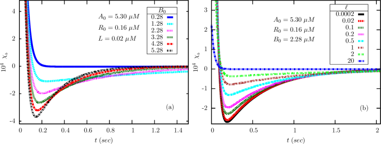
Refer to caption
Figure 10: The bilobed chemotactic response function Ο‡b​(t)subscriptπœ’π‘π‘‘\chi_{b}(t) (59) as a function of time obtained for various values of (a) methylesterase CheB (B0subscript𝐡0B_{0}) and (b) ligand (β„“=L/KLℓ𝐿subscript𝐾𝐿\ell=L/K_{L}) concentrations. In (a), we have fixed β„“=0.2β„“0.2\ell=0.2. All other (fixed) parameters take the values mentioned in Table1. We have also used Ξ»Y=30​sβˆ’1subscriptπœ†π‘Œ30superscript𝑠1\lambda_{Y}=30s^{-1} [15, 31, 14], H=20𝐻20H=20 [16] and PCW​(Yβˆ—)=0.5subscript𝑃CWsuperscriptπ‘Œ0.5P_{\rm CW}(Y^{*})=0.5.

6.4 On the role of biochemical noise in the run and tumble motion of E.coli

From (56), it follows that a fluctuation in [CheYp] equal to its standard deviation in magnitude would cause the following change in PCWsubscript𝑃CWP_{\rm{CW}}:

δ​PCW=HKY​yΒ―(Hβˆ’1)(1+yΒ―H)2​σY𝛿subscript𝑃CW𝐻subscriptπΎπ‘Œsuperscript¯𝑦𝐻1superscript1superscript¯𝑦𝐻2subscriptπœŽπ‘Œ\delta P_{\rm{CW}}=\frac{H}{K_{Y}}\frac{\overline{y}^{(H-1)}}{(1+\overline{y}^{H})^{2}}\sigma_{Y} (62)

where y=Y/KYπ‘¦π‘ŒsubscriptπΎπ‘Œy=Y/K_{Y} and y¯¯𝑦\overline{y} is its mean value in steady state. The function yΒ―Hβˆ’1/(1+yΒ―H)2superscript¯𝑦𝐻1superscript1superscript¯𝑦𝐻2\overline{y}^{H-1}/(1+\overline{y}^{H})^{2} has a single maximum (and no minimum) at yΒ―=[(Hβˆ’1)/(H+1)]1/H≑y~¯𝑦superscriptdelimited-[]𝐻1𝐻11𝐻~𝑦\overline{y}=[(H-1)/(H+1)]^{1/H}\equiv\tilde{y}, with maximum value 1/4 for H≫1much-greater-than𝐻1H\gg 1. Using this property in (62) leads to the following upper bound on δ​PCW𝛿subscript𝑃CW\delta P_{\rm{CW}}:

δ​PCW≀H4​KY​σY𝛿subscript𝑃CW𝐻4subscriptπΎπ‘ŒsubscriptπœŽπ‘Œ\delta P_{\rm{CW}}\leq\frac{H}{4K_{Y}}\sigma_{Y} (63)

The standard deviation ΟƒYsubscriptπœŽπ‘Œ\sigma_{Y} has been measured in experiments, and the range of variation has been estimated[28] as

0.09<ΟƒY<0.22,0.09subscriptπœŽπ‘Œ0.220.09<\sigma_{Y}<0.22, (64)

with the actual value depending on the mean clockwise bias, PΒ―CWsubscript¯𝑃CW{\overline{P}}_{\rm CW}. The dissociation constant KY≃3​μ​Msimilar-to-or-equalssubscriptπΎπ‘Œ3πœ‡π‘€K_{Y}\simeq 3\mu M and the Hill coefficient H≃20similar-to-or-equals𝐻20H\simeq 20 (for pre-adapted motors) have also been measured in single cell experiments [16]. Using this estimate in (63), we find δ​PCW≀0.15βˆ’0.367𝛿subscript𝑃CW0.150.367\delta P_{\rm CW}\leq 0.15-0.367 (assuming yΒ―β‰ˆy~¯𝑦~𝑦\overline{y}\approx\tilde{y}). So there is a maximum fluctuation of 18%percent1818\% for H=20𝐻20H=20 corresponding to a CW bias of 0.50.50.5 and [CheYp] ∼3​μ​Msimilar-toabsent3πœ‡π‘€\sim 3\mu M around which the transition becomes ultrasensitive. Therefore, the fluctuations in [CheYp] appear sufficiently large to affect the switching behavior of the motor.

Next, how large the fluctuations in activity need to be, to produce the observed standard deviation in [CheYp]? The following simple picture helps us to obtain an estimate. In E.coli, active receptors undergo autophosphorylation, and then transfer the phosphoryl groups to the proteins CheB and CheY. For simplicity, we ignore phosphorylation of CheB and focus on CheY. The dynamics of Y​(t)π‘Œπ‘‘Y(t) is expressed in (53). Under steady state conditions, the variance ΟƒY2=⟨Y2βŸ©βˆ’βŸ¨Y⟩2superscriptsubscriptπœŽπ‘Œ2delimited-⟨⟩superscriptπ‘Œ2superscriptdelimited-βŸ¨βŸ©π‘Œ2\sigma_{Y}^{2}=\langle Y^{2}\rangle-\langle Y\rangle^{2} is given by the expression

ΟƒY2=(aY​Y0​A0)2Ξ»Y​(Ξ»Y+λξ)​σa2superscriptsubscriptπœŽπ‘Œ2superscriptsubscriptπ‘Žπ‘Œsubscriptπ‘Œ0subscript𝐴02subscriptπœ†π‘Œsubscriptπœ†π‘Œsubscriptπœ†πœ‰superscriptsubscriptπœŽπ‘Ž2\sigma_{Y}^{2}=\frac{(a_{Y}Y_{0}A_{0})^{2}}{\lambda_{Y}(\lambda_{Y}+\lambda_{\xi})}\sigma_{a}^{2} (65)

where, we have introduced the correlation length λξsubscriptπœ†πœ‰\lambda_{\xi} for the fluctuations in ΞΎasubscriptπœ‰π‘Ž\xi_{a}, defined through the relation βŸ¨Ξ΄β€‹ΞΎa​(t)​δ​ξa​(tβ€²)⟩=Οƒa2​exp⁑(βˆ’Ξ»ΞΎβ€‹|tβˆ’tβ€²|)delimited-βŸ¨βŸ©π›Ώsubscriptπœ‰π‘Žπ‘‘π›Ώsubscriptπœ‰π‘Žsuperscript𝑑′superscriptsubscriptπœŽπ‘Ž2subscriptπœ†πœ‰π‘‘superscript𝑑′\langle\delta\xi_{a}(t)\delta\xi_{a}(t^{\prime})\rangle=\sigma_{a}^{2}\exp(-\lambda_{\xi}|t-t^{\prime}|) in steady state, where δ​ξa​(t)=ΞΎa​(t)βˆ’ΞΎa¯𝛿subscriptπœ‰π‘Žπ‘‘subscriptπœ‰π‘Žπ‘‘Β―subscriptπœ‰π‘Ž\delta\xi_{a}(t)=\xi_{a}(t)-\overline{\xi_{a}} is the fluctuation in activity relative to its steady state value. From (65), the inequality

ΟƒY≀aY​Y0​A0Ξ»Y​σasubscriptπœŽπ‘Œsubscriptπ‘Žπ‘Œsubscriptπ‘Œ0subscript𝐴0subscriptπœ†π‘ŒsubscriptπœŽπ‘Ž\sigma_{Y}\leq\frac{a_{Y}Y_{0}A_{0}}{\lambda_{Y}}\sigma_{a} (66)

follows, the equality being satisfied in the limit λξβ‰ͺΞ»Ymuch-less-thansubscriptπœ†πœ‰subscriptπœ†π‘Œ\lambda_{\xi}\ll\lambda_{Y} (which we shall assume henceforth). Various estimates for the parameters in (66) are available in the literature (see Table2). Using (64), we identify the following ranges for the standard deviation ΟƒasubscriptπœŽπ‘Ž\sigma_{a} of receptor activity:

4.7Γ—10βˆ’34.7superscript103\displaystyle 4.7\times 10^{-3} <\displaystyle< Οƒa<10βˆ’2(i)subscriptπœŽπ‘Žsuperscript102i\displaystyle\sigma_{a}<10^{-2}\;\;\;\;\;\;\;\;\;\;\;\;\;\rm{(i)}
3Γ—10βˆ’43superscript104\displaystyle 3\times 10^{-4} <\displaystyle< Οƒa<7.4Γ—10βˆ’4​(ii)subscriptπœŽπ‘Ž7.4superscript104ii\displaystyle\sigma_{a}<7.4\times 10^{-4}\;\;\;\rm{(ii)}
5.2Γ—10βˆ’45.2superscript104\displaystyle 5.2\times 10^{-4} <\displaystyle< Οƒa<10βˆ’3(iii)subscriptπœŽπ‘Žsuperscript103iii\displaystyle\sigma_{a}<10^{-3}\;\;\;\;\;\;\;\;\;\;\;\rm{(iii)} (67)

It is also of interest to compare the values of the ZOU parameter α𝛼\alpha across these sets of parameters, which turn out to be 0.547 (i), 0.076 (ii) and 0.035 (iii) (Table2). Note that the estimated variance in (ii) and (iii) are smaller than (i), which is consistent with our expectation of maximum variance near Ξ±=1𝛼1\alpha=1, over a large range of values of β„“β„“\ell. The magnitude of receptor noise predicted by (6.4) also agrees with our predictions (see Fig (3), also Fig (8)).

Table 2: A list of relevant parameter values collected from the literature.
Numerical values
Symbol Quantity Morton-Firth et al. [32] Rao et al.[31] Kollmann et al.[14]
aYsubscriptπ‘Žπ‘Œa_{Y} CheY phosphorylation rate 3 μ​Mβˆ’1​sβˆ’1πœ‡superscript𝑀1superscript𝑠1\mu M^{-1}s^{-1} 100 μ​Mβˆ’1​sβˆ’1πœ‡superscript𝑀1superscript𝑠1\mu M^{-1}s^{-1} 100 μ​Mβˆ’1​sβˆ’1πœ‡superscript𝑀1superscript𝑠1\mu M^{-1}s^{-1}
Ξ»Ysubscriptπœ†π‘Œ\lambda_{Y} CheYp dephosphorylation rate 14.15 sβˆ’1superscript𝑠1s^{-1} 30.1 sβˆ’1superscript𝑠1s^{-1} 30.1 sβˆ’1superscript𝑠1s^{-1}
Y0subscriptπ‘Œ0Y_{0} CheY concentration 18 ΞΌπœ‡\muM 17.9 ΞΌπœ‡\muM 9.7 ΞΌπœ‡\muM
A0subscript𝐴0A_{0} CheA concentration 5 ΞΌπœ‡\muM 5 ΞΌπœ‡\muM 5.3 ΞΌπœ‡\muM
R0subscript𝑅0R_{0} CheR concentration 0.235 ΞΌπœ‡\muM 0.3 ΞΌπœ‡\muM 0.16 ΞΌπœ‡\muM
B0subscript𝐡0B_{0} CheB concentration 2.27 ΞΌπœ‡\muM 2 ΞΌπœ‡\muM 0.28 ΞΌπœ‡\muM
Ξ½rsubscriptπœˆπ‘Ÿ\nu_{r} Methylation rate 0.819 sβˆ’1superscript𝑠1s^{-1} 0.255 sβˆ’1superscript𝑠1s^{-1} 0.39 sβˆ’1superscript𝑠1s^{-1}
Ξ½bsubscriptπœˆπ‘\nu_{b} Demethylation rate 0.155 sβˆ’1superscript𝑠1s^{-1} 0.5 sβˆ’1superscript𝑠1s^{-1} 6.3 sβˆ’1superscript𝑠1s^{-1}
α​(29)𝛼29\alpha(\ref{alpha}) ZOU parameter 0.547 0.076 0.035

6.5 Effect of flagellar motor level adaptation on fluctuations in clockwise bias

From the experimental data of Yuan and Berg (2013) [16], we propose that the change in clockwise bias in response to a time-dependent change in [CheYp] (denoted δ​Y​(t)π›Ώπ‘Œπ‘‘\delta Y(t) henceforth) be written in the general linear form

δ​PCW​(t)=βˆ«βˆ’βˆžtΟ‡m​(tβˆ’tβ€²)​δ​Y​(tβ€²)​𝑑t′𝛿subscript𝑃CW𝑑superscriptsubscript𝑑subscriptπœ’π‘šπ‘‘superscriptπ‘‘β€²π›Ώπ‘Œsuperscript𝑑′differential-dsuperscript𝑑′\delta P_{\rm CW}(t)=\int_{-\infty}^{t}\chi_{m}(t-t^{\prime})\delta Y(t^{\prime})dt^{\prime} (68)

where Ο‡m​(Ο„)subscriptπœ’π‘šπœ\chi_{m}(\tau) (defined for Ο„>0𝜏0\tau>0) is the linear response function for the motor, which we assume to consist of two terms:

Ο‡m​(Ο„)=Ξ±na​δ​(Ο„)+Γ​eβˆ’Ξ»m​τsubscriptπœ’π‘šπœsubscript𝛼naπ›ΏπœΞ“superscript𝑒subscriptπœ†π‘šπœ\chi_{m}(\tau)=\alpha_{\rm na}\delta(\tau)+\Gamma e^{-\lambda_{m}\tau} (69)

where Ξ±na=βˆ‚YPCWnasubscript𝛼nasubscriptπ‘Œsuperscriptsubscript𝑃CWna\alpha_{\rm na}=\partial_{Y}P_{\rm CW}^{\rm na}, and PCWnasuperscriptsubscript𝑃CWnaP_{\rm CW}^{\rm na} is the bias of the non-adapted motor, as measured by Yuan and Berg (2013), with Hill coefficient Hβ‰ˆ20𝐻20H\approx 20. The second term represents the slow change in the bias originating from motor-level adaptation, with Ξ»mβˆ’1superscriptsubscriptπœ†π‘š1\lambda_{m}^{-1} being the time scale for the same. Now, for a step-like change in Yπ‘ŒY such that Yβ†’Y0+Δ​Yβ†’π‘Œsubscriptπ‘Œ0Ξ”π‘ŒY\to Y_{0}+\Delta Y at t=0𝑑0t=0, let us put δ​Y​(t)=Δ​Yβ€‹Ξ˜β€‹(t)π›Ώπ‘Œπ‘‘Ξ”π‘ŒΞ˜π‘‘\delta Y(t)=\Delta Y\Theta(t); using this in (68) yields the response for the same:

δ​PCWstep​(t)=Δ​Yβ€‹βˆ«0tΟ‡m​(Ο„)​𝑑τ𝛿superscriptsubscript𝑃CWstepπ‘‘Ξ”π‘Œsuperscriptsubscript0𝑑subscriptπœ’π‘šπœdifferential-d𝜏\delta P_{\rm CW}^{\rm step}(t)=\Delta Y\int_{0}^{t}\chi_{m}(\tau)d\tau (70)

As tβ†’βˆžβ†’π‘‘t\to\infty, the system will adapt, and hence δ​PCWstep​(t)β†’Ξ±a​Δ​Y→𝛿superscriptsubscript𝑃CWstep𝑑subscript𝛼aΞ”π‘Œ\delta P_{\rm CW}^{\rm step}(t)\to\alpha_{\rm a}\Delta Y, where Ξ±a=βˆ‚YPCWasubscript𝛼asubscriptπ‘Œsuperscriptsubscript𝑃CWa\alpha_{\rm a}=\partial_{Y}P_{\rm CW}^{\rm a}, and PCWasuperscriptsubscript𝑃CWaP_{\rm CW}^{\rm a} is the clockwise bias of the adapted motor. From (69), it then follows that Ξ“=λ​(Ξ±aβˆ’Ξ±na)Ξ“πœ†subscript𝛼asubscript𝛼na\Gamma=\lambda(\alpha_{\rm a}-\alpha_{\rm na}). Let us now compute the effect on the CW bias of random fluctuations in Yπ‘ŒY, and define the root-mean square change of bias by δ​PCWβ‰‘βŸ¨Ξ΄β€‹PCW​(t)⟩2𝛿subscript𝑃CWsuperscriptdelimited-βŸ¨βŸ©π›Ώsubscript𝑃CW𝑑2\delta P_{\rm CW}\equiv\sqrt{\langle\delta P_{\rm CW}(t)\rangle^{2}}, with the average to be carried out over different realizations of the fluctuations in [CheYp]. From (68), it turns out that

βŸ¨Ξ΄β€‹PCW​(t)⟩2=βˆ«βˆ’βˆžt𝑑t1β€‹βˆ«βˆ’βˆžt𝑑t2​χm​(tβˆ’t1)​χm​(tβˆ’t2)β€‹βŸ¨Ξ΄β€‹Y​(t1)​δ​Y​(t2)⟩,superscriptdelimited-βŸ¨βŸ©π›Ώsubscript𝑃CW𝑑2superscriptsubscript𝑑differential-dsubscript𝑑1superscriptsubscript𝑑differential-dsubscript𝑑2subscriptπœ’π‘šπ‘‘subscript𝑑1subscriptπœ’π‘šπ‘‘subscript𝑑2delimited-βŸ¨βŸ©π›Ώπ‘Œsubscript𝑑1π›Ώπ‘Œsubscript𝑑2\langle\delta P_{\rm CW}(t)\rangle^{2}=\int_{-\infty}^{t}dt_{1}\int_{-\infty}^{t}dt_{2}\chi_{m}(t-t_{1})\chi_{m}(t-t_{2})\langle\delta Y(t_{1})\delta Y(t_{2})\rangle, (71)

where, in steady state, we expect βŸ¨Ξ΄β€‹Y​(t1)​δ​Y​(t2)⟩=ΟƒY2​eβˆ’Ξ»Y​(t1βˆ’t2)delimited-βŸ¨βŸ©π›Ώπ‘Œsubscript𝑑1π›Ώπ‘Œsubscript𝑑2superscriptsubscriptπœŽπ‘Œ2superscript𝑒subscriptπœ†π‘Œsubscript𝑑1subscript𝑑2\langle\delta Y(t_{1})\delta Y(t_{2})\rangle=\sigma_{Y}^{2}e^{-\lambda_{Y}(t_{1}-t_{2})} for t1>t2subscript𝑑1subscript𝑑2t_{1}>t_{2}, ΟƒY2subscriptsuperscript𝜎2π‘Œ\sigma^{2}_{Y} is the steady state variance of Yπ‘ŒY as given by (65) and Ξ»Ysubscriptπœ†π‘Œ\lambda_{Y} is the dephosphorylation rate of [CheYp]. Using the expression for Ο‡m​(t)subscriptπœ’π‘šπ‘‘\chi_{m}(t) from (69) and completing the calculations yields the final result

δ​PCW=ΟƒY​αna​[1βˆ’Ξ»mΞ»Y​αaΞ±na​(1βˆ’Ξ±aΞ±na)]𝛿subscript𝑃CWsubscriptπœŽπ‘Œsubscript𝛼nadelimited-[]1subscriptπœ†π‘šsubscriptπœ†π‘Œsubscript𝛼asubscript𝛼na1subscript𝛼asubscript𝛼na\delta P_{\rm CW}=\sigma_{Y}\alpha_{\rm na}\sqrt{\left[1-\frac{\lambda_{m}}{\lambda_{Y}}\frac{\alpha_{\rm a}}{\alpha_{\rm na}}\left(1-\frac{\alpha_{\rm a}}{\alpha_{\rm na}}\right)\right]} (72)

The term outside the square root is precisely the result in (62) in 6.3. Explicit evaluation of the term in brackets (see Fig.11) shows, however, that the contribution of motor-level adaptation to the fluctuations in bias is negligible in the sensitive part of the response curve.
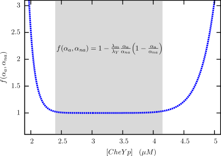
Refer to caption
Figure 11: The term inside the square root in (72) is plotted against Yπ‘ŒY. Note the flat region, nearly 1.5μ​Mπœ‡π‘€\mu M in width, where the correction arising from motor-level adaptation is negligible. Ξ±asubscriptπ›Όπ‘Ž\alpha_{a} and Ξ±n​asubscriptπ›Όπ‘›π‘Ž\alpha_{na} have been computed from (56) with Ha=10subscriptπ»π‘Ž10H_{a}=10 [17] and Hn​a=20subscriptπ»π‘›π‘Ž20H_{na}=20 [16]. We have taken Ξ»m=0.0167​sβˆ’1subscriptπœ†π‘š0.0167superscript𝑠1\lambda_{m}=0.0167s^{-1} considering that motor adaptation takes place over a minute [24] and Ξ»Y=30​sβˆ’1subscriptπœ†π‘Œ30superscript𝑠1\lambda_{Y}=30s^{-1} [31, 14].

Acknowledgments

We thank P.G. Senapathy Centre for Computing Resources, IIT Madras, for providing us with computing facilities in the Virgo cluster.

References

  • [1] Goldbeter A, Koshland Jr DE. An amplified sensitivity arising from covalent modification in biological systems. Proc. Natl. Acad. Sci. 1981 73(11):6840-6844.
  • [2] Jithinraj PK, Roy U, Gopalakrishnan M. Zero-order ultrasensitivity: A study of criticality and fluctuations under the total quasi-steady state approximation in the linear noise regime. J. Theor. Biol. 2014 344:1-11.
  • [3] Berg OG, Paulsson J, Ehrenberg M. Fluctuations and quality of control in biological cells: zero-order ultrasensitivity reinvestigated. Biophys. J. 2000 79:1228–1236.
  • [4] Elf J, Ehrenberg M. Fast evaluation of fluctuations in biochemical networks with the linear noise approximation. Genome Res. 2003 13:2475–2484.
  • [5] Xu Y, Gunawardena J. Realistic enzymology for post-translational modification: zero-order ultrasensitivity revisited. J. Theor. Biol. 2012 311:139–152.
  • [6] Qian H. Thermodynamic and kinetic analysis of sensitivity amplification in biological signal transduction. Biophys. Chem. 2003 105:585–593.
  • [7] Ge H, Qian M. Sensitivity amplification in the phosphorylation–dephosphorylation cycle: nonequilibrium steady states, chemical master equation, and temporal cooperativity. J. Chem. Phys. 2008 129:015104.
  • [8] Tindall MJ, Porter SL, Maini PK, Gaglia G, Armitage JP. Overview of mathematical approaches used to model bacterial chemotaxis I: the single cell. Bull. Math. Biol. 2008 70: 1525-1569.
  • [9] Segall JE, Block SM, Berg HC. Temporal comparisons in bacterial chemotaxis. Proc. Natl. Acad. Sci. USA 1986 83:8987–8991.
  • [10] Barkai N, Leibler S. Robustness in simple biochemical networks. Nature. 1997 387: 913-917.
  • [11] Rao CV, Kirby JR, Arkin AP. Design and Diversity in Bacterial Chemotaxis: A Comparative Study in Escherichia coli and Bacillus subtilis. PLoS Biol. 2004 2:E49.
  • [12] Pontius W, Sneddon MW, Emonet T. Adaptation dynamics in densely clustered chemoreceptors. PLoS Comp. Biol. 2013 9(9): e1003230
  • [13] Mello D, Tu Y. Perfect and near-perfect adaptation in a model of bacterial chemotaxis. Biophys. J. 2003 84:2943-2956.
  • [14] Kollmann M, Lovdok L, Bartholome K, Timmer J, Sourjik, V. (2005) Design principles of a bacterial signalling network. Nature 2005 438: 504-507
  • [15] Reneaux M, Gopalakrishnan M. Theoretical results for chemotactic response and drift of E. coli in a weak attractant gradient. J. Theor. Biol. 2010 266:99–106.
  • [16] Yuan J, Berg HC. Ultrasensitivity of an adaptive bacterial motor. J. Mol. Biol. 2013 425: 1760-1764
  • [17] Cluzel P, Surette M, Leibler S. An ultrasensitive bacterial motor revealed by monitoring signaling proteins in single cells. Science. 2000. 287: 1652-1655.
  • [18] Asakura S, Honda M. Two-state model for bacterial chemoreceptor proteins: the role of multiple methylation. J. Math. Biol. 1984 176:349–367.
  • [19] Emonet T, Cluzel P. Relationship between cellular response and behavioural variability in bacterial chemotaxis. Proc. Nat. Acad. Sci. USA 2008 105:3304–3309.
  • [20] Sourjik V, Berg HC. Receptor sensitivity in bacterial chemotaxis. Proc. Nat. Acad. Sci. USA 2002 99: 123-127.
  • [21] Schnoerr D, Sanguinetti G, Grima R. Approximation and inference methods for stochastic biochemical kinetics - a tutorial review. J. Phys. A: Math. Theor. 2016 10.1088: 1751-8121
  • [22] van Kampen NG. Stochastic Processes in Physics and Chemistry. Elsevier. 2007
  • [23] Gillespie DT. Exact stochastic simulation of coupled chemical reactions. J. Phys. Chem. 1977 81(25):2340-2351.
  • [24] Yuan J, Branch RW, Hosu BG, Berg HC. Adaptation at the output of the chemotaxis signalling pathway. Nature 2012 484: 233-236
  • [25] Lipkow K. Changing cellular localization of CheZ predicted by molecular simulations. PLoS Comput. Biol. 2006 2, e39
  • [26] Endres RG, Wingreen NS Precise adaptation in bacterial chemotaxis through β€œassistance neighbourhoods”. Proc. Natl. Acad. Sci. USA 2006 103: 13040-13044
  • [27] Hansen CH, Endres RG, Wingreen NS Chemotaxis in Escherichia coli: a molecular model for robust precise adaptation. PLos Comp. Biol. 2008 4: e1
  • [28] Park H, Pontius W,Guet CC, Marko JF, Emonet T, Cluzel P. Interdependence of behavioural variability and response to small stimuli in bacteria. Nature 2010 468:819-823
  • [29] Park H, Oikonomou P, Guet CC, Cluzel P. Noise underlies switching behaviour of the bacterial flagellum. Biophys. J. 2011 101(10): 2336-2340
  • [30] Masson JB, Voisinnea G, Wong-Nga J, Celani A and Vergassola M Noninvasive inference of the molecular chemotactic response using bacterial trajectories. Proc. Natl. Acad. Sci. USA 2012 109: 1802–1807
  • [31] Rao CV, Arkin AP. Stochastic chemical kinetics and the quasi-steady-state assumption: Application to the Gillespie algorithm. J. Chem. Phys. 2003 118: 4999-5010
  • [32] Morton-Firth CJ, Shimizu TS, Bray D. A free-energy-based stochastic simulation of the Tar receptor complex. J. Mol. Biol. 1999 286: 1059-1074