Almost all four-particle pure states are determined
by their two-body marginals

Abstract

We show that generic pure states (states drawn according to the Haar measure) of four particles of equal internal dimension are uniquely determined among all other pure states by their two-body marginals. In fact, certain subsets of three of the two-body marginals suffice for the characterization. We also discuss generalizations of the statement to pure states of more particles, showing that these are almost always determined among pure states by three of their $(n-2)$-body marginals. Finally, we present special families of symmetric pure four-particle states that share the same two-body marginals and are therefore undetermined. These are four-qubit Dicke states in superposition with generalized GHZ states.

Introduction. The question of what can be learned about a multiparticle system by looking at some particles only is central for many problems in physics. In quantum mechanics, this problem can be formulated in a mathematical fashion as follows: Given a quantum state $\rho$ on $n$ particles, which properties of this state can be inferred from knowledge of the $k$-particle reduced states only? This question is naturally connected to the phenomenon of entanglement. Indeed, considering pure states of two-particles, product states are always determined by their marginals, whereas entangled states can exhibit reduced states that admit multiple compatible joint states. Consequently, entangled states may contain information in correlations among many parties that is lost when just having access to the reductions. In fact, many works have considered the problem how entanglement or other global properties relate to properties of the reduced states Tóth et al. (2009); Würflinger et al. (2012); Walter et al. (2013); Miklin, Moroder, and Gühne (2016). On a more fundamental level, one may ask the question whether for a given set of reduced states the original global state is the only state having this set of reduced states Coleman (1963); Klyachko ; Sawicki, Walter, and Kus (2013); Schilling, Benavides-Riveros, and Vrana .

This question is also of practical interest: If a quantum state happens to be the unique ground state of a Hamiltonian, it may be obtained by engineering this Hamiltonian and then cooling down the system. In practice, typical Hamiltonians are limited to having interactions between two or three particles only. The question of whether the ground state of such a Hamiltonian is unique is then directly related to the question of whether the state one wants to prepare is uniquely determined by its two- or three-body marginals (Zhou, 2009; Huber and Gühne, 2016).

The question of uniqueness was analyzed in detail by Linden and coworkers, who showed that almost all pure three-qubit states are determined among all mixed states by their two-body marginals (Linden, Popescu, and Wootters, 2002). Later, Diósi showed that two of the three two-body marginals suffice to characterize uniquely a pure three-particle state among all other pure states (Diósi, 2004). Jones and Linden finally proved that generic states of $n$ qudits are uniquely determined by certain sets of reduced states of just more than half of the parties, whereas the reduced states of fewer than half of the parties are not sufficient (Jones and Linden, 2005). Thus, higher-order correlations of most pure quantum states are not independent of the lower-order correlations.

In this paper, we investigate the case of four-particle states having equal internal dimension. We show that generic pure states of four particles are uniquely determined among all pure states by certain sets of their two-body marginals. To that end, we begin by defining what we mean by generic states and distinguish the different kinds of uniqueness, namely uniqueness among pure and uniqueness among all states. We then prove our main result, first for the case of qubits and subsequently the general case of qudits. The theorem is then generalized to generic $n$-particle states, which can be shown to be determined in a similar way by certain sets of three of their $(n-2)$-body marginals. Finally, we list some specific examples for the exceptional case of states of four particles that are not determined by their two-body marginals.

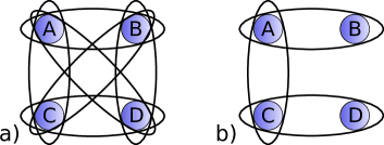
Figure 1: Illustration of two different sets of two-body marginals: a) the set of all six two-body marginals, b) a set of three two-body marginals that is shown to suffice to uniquely determine pure generic pure states.

Random states and uniqueness. We begin with some basic definitions. Given an $n$-particle quantum state $\rho$ of parties $\mathcal{P}=\{P_{1},\ldots,P_{n}\}$, its $k$-body marginal of parties $\mathcal{S}=\{P_{i_{1}},\ldots,P_{i_{k}}\}$ is defined as

$$\rho_{\mathcal{S}}:=\operatorname{Tr}_{\bar{\mathcal{S}}}(\rho)\>,$$ (1)

where the trace is a partial trace over parties $\bar{\mathcal{S}}=\mathcal{P}\setminus\mathcal{S}$. When stating the question of uniqueness, i.e., whether a given state is uniquely determined by some of its marginals, it is important to specify the set of states considered. Usually, two different sets are taken into account, namely the set of pure states and the set of all states, leading to two different kinds of uniqueness, namely that of uniqueness among pure states (UDP) and uniqueness among all states (UDA). We adopt here the definition of Ref. (Chen et al., 2013) and extend it by specifying which marginals are involved:

Definition 1.

A state $\ket{\psi}$ is called

• $k$-uniquely determined among pure states ($k$-UDP), if there exists no other pure state having the same $k$-body marginals as $\ket{\psi}$.

• $k$-uniquely determined among all states ($k$-UDA), if there exists no other state (mixed or pure) having the same $k$-body marginals as $\ket{\psi}$.

Using this language, the results of Ref. (Linden, Popescu, and Wootters, 2002) show that almost all three-qubit pure states are $2$-UDA, that is, given a random pure state $\ket{\psi}$, it is uniquely determined by its marginals $\rho_{\text{AB}}$, $\rho_{\text{AC}}$ and $\rho_{\text{BC}}$. Ref. (Diósi, 2004) states that knowledge of just two of the three two-body marginals suffices to fix the state among all pure states (UDP). Later, these results were generalized to states of certain higher internal dimensions, for a more general overview see for example Ref. (Chen et al., 2013). Note that while UDA implies UDP, the converse in general does not need to be true and there are examples of four-qubit states which are 2-UDP but not 2-UDA (Xin et al., 2017). Other cases of UDP versus UDA are discussed in Ref. (Chen et al., 2013).

Note that in some cases a subset of all $k$-body marginals already suffices to show uniqueness, as in the case of almost all three-qubit states discussed above (Diósi, 2004). In this paper, we will show that in case of four particles, specific sets consisting of three of the six two-body marginals suffice to determine any generic pure states among all pure states.

Generic states are understood to be states drawn randomly according to the Haar measure. Here, we adopt a special procedure to obtain such random states in a Schmidt decomposed form. To that end, consider a four-particle pure state $\ket{\psi}\in\mathcal{H}_{A}\otimes\mathcal{H}_{B}\otimes\mathcal{H}_{C}\otimes\mathcal{H}_{D}$, where $\dim\mathcal{H}_{A}=\dim\mathcal{H}_{B}=\ldots=d$. Using the Schmidt decomposition along the bipartition ($AB|CD$), the state can be written as

$$\ket{\psi}=\sum_{i=1}^{d^{2}}\sqrt{\lambda_{i}}\ket{i}_{\text{AB}}\otimes\ket{i}_{\text{CD}},$$ (2)

where $\sum_{i}\lambda_{i}=1$. If the state has full Schmidt rank, i.e., $\lambda_{i}\neq 0$ for all $i$, then the sets $\ket{i}_{\text{AB}}$ and $\ket{i}_{\text{CD}}$ form orthonormal bases in the composite Hilbert spaces $\mathcal{H}_{A}\otimes\mathcal{H}_{B}$ and $\mathcal{H}_{C}\otimes\mathcal{H}_{D}$, respectively.

Definition 2.

A generic four-particle pure state is a state $\ket{\psi}\in\mathcal{H}_{A}\otimes\mathcal{H}_{B}\otimes\mathcal{H}_{C}\otimes\mathcal{H}_{D}$ drawn randomly according to the Haar measure. Writing such state as in Eq. (2), the Schmidt bases and the set of Schmidt coefficients are independent from each other. The distribution of the Schmidt coefficients is given by (Scott and Caves, 2003; Lloyd and Pagels, 1988)

$$P(\lambda_{1},\ldots,\lambda_{d^{2}})\text{d}\lambda_{1}\ldots\text{d}\lambda_{d^{2}}\\ =N\delta\left(1-\sum_{i=1}^{d^{2}}\lambda_{i}\right)\prod_{1\leq i<j\leq d^{2}}(\lambda_{i}-\lambda_{j})^{2}\text{d}\lambda_{1}\ldots\text{d}\lambda_{d^{2}}$$ (3)

and the Schmidt bases are distributed according to the Haar measure of unitary operators on the smaller Hilbert spaces.

The mutual independence of the two Schmidt bases and the coefficients can be seen from the fact that in the Haar measure, for the probability distribution $p(\ket{\psi})$ to obtain state $\ket{\psi}$ holds $p(\ket{\psi})=p(\mathds{1}_{\text{AB}}\otimes U_{\text{CD}}\ket{\psi})=p(U_{\text{AB}}\otimes\mathds{1}_{\text{CD}}\ket{\psi})$.

Generic states as defined above exhibit two other important properties: They have full Schmidt rank and pairwise distinct Schmidt coefficients. We would like to add that while the definition above makes use of the Haar measure, we do not explicitly require it. Any measure with the same independence properties between the two Schmidt bases and Schmidt coefficients would work as well, as long as the sets of states having non-full Schmidt rank or degenerate Schmidt coefficients are also of measure zero.

The case of qubits. To begin with, we investigate the qubit case, where $d=2$. Let $\ket{\psi}=\sum_{i=1}^{4}\sqrt{\lambda_{i}}\ket{i}_{\text{AB}}\otimes\ket{i}_{\text{CD}}$ be a generic state in the sense defined above. The two-body marginal of parties $A$ and $B$ is given by

$$\rho_{\text{AB}}=\operatorname{Tr}_{\text{CD}}(\ket{\psi}\!\bra{\psi})=\sum_{i=1}^{4}\lambda_{i}\ket{i}\!\bra{i}_{\text{AB}}$$ (4)

and similarly for $CD$. This is the starting point for the proof of the following theorem.

Theorem 3.

Almost all four-qubit pure states are uniquely determined among pure states by the three two-body marginals $\rho_{\text{AB}}$, $\rho_{\text{CD}}$ and $\rho_{\text{BD}}$. In particular, this implies that they are $2$-UDP.

Proof.

Let $\ket{\psi}$ be a generic state in the Schmidt decomposed form in Eq. (2). We arrange the Schmidt bases such that the Schmidt coefficients are in decreasing order, i.e. $\lambda_{i}\geq\lambda_{i+1}$. Suppose that there is another pure state $\ket{\phi}$ which exhibits the same two-body marginals $\rho_{\text{AB}}$ and $\rho_{\text{CD}}$ as $\ket{\psi}$. As the $\lambda_{i}$ are pairwise distinct and in decreasing order, the Schmidt bases of $\ket{\phi}$ and $\ket{\psi}$ have to coincide up to a phase. Thus, $\ket{\phi}$ must be of the form

$$\ket{\phi}=\sum_{i=1}^{4}e^{i\varphi_{i}}\sqrt{\lambda_{i}}\ket{i}_{\text{AB}}\otimes\ket{i}_{\text{CD}}.$$ (5)

Therefore, the only degrees of freedom left of $\ket{\phi}$ are the four phases $\varphi_{i}$.

We now demand that also the marginals of parties $B$ and $D$ coincide, i.e. $\operatorname{Tr}_{\text{AC}}(\ket{\psi}\!\bra{\psi})=\operatorname{Tr}_{\text{AC}}(\ket{\phi}\!\bra{\phi})$ (but any other marginal would be fine, too):

$$\!\!\!\rho_{\text{BD}} \!=\!\! \sum_{i,j=1}^{4}\!\!\sqrt{\lambda_{i}\lambda_{j}}\operatorname{Tr}_{\text{AC}}(\ket{i}\!\bra{j}_{\text{AB}}\otimes\ket{i}\!\bra{j}_{\text{CD}})$$ (6)

$$\!\overset{!}{=}\!\! \sum_{i,j=1}^{4}\!\!e^{i(\varphi_{i}-\varphi_{j})}\sqrt{\lambda_{i}\lambda_{j}}\operatorname{Tr}_{\text{AC}}(\ket{i}\!\bra{j}_{\text{AB}}\otimes\ket{i}\!\bra{j}_{\text{CD}})\text{.}$$

The sum runs over operators on the space of parties $B$ and $D$. For every pair $i,j$, this operator is given by

$$O_{ij}=\operatorname{Tr}_{\text{AC}}(\ket{i}\!\bra{j}_{\text{AB}}\otimes\ket{i}\!\bra{j}_{\text{CD}}).$$ (7)

The 16 operators $O_{ij}$ span a subspace in the 16-dimensional space of operators on $\mathcal{H}_{B}\otimes\mathcal{H}_{D}$. As we will see later, this subspace is only 13-dimensional, thus the operators must be linearly dependent. Therefore, we cannot simply compare both sides of Eq. (6) term by term to conclude that $\varphi_{i}=\varphi_{j}$. Instead, let us interpret the 16 operators $O_{ij}$ as vectors in the 16-dimensional operator space. Thus, we are looking for solutions of the equation

$$\sum_{i,j=1}^{4}(1-e^{i(\varphi_{i}-\varphi_{j})})\sqrt{\lambda_{i}\lambda_{j}}O_{ij}\equiv\sum_{i,j=1}^{4}\gamma_{ij}O_{ij}=0_{4\times 4}\>,$$ (8)

where

$$\gamma_{ij}:=(1-e^{i(\varphi_{i}-\varphi_{j})})\sqrt{\lambda_{i}\lambda_{j}}\>\text{.}$$ (9)

These are 16 equations, one for every entry of the resulting $4\times 4$ matrix. We can treat Eq. (8) as a system of linear equations for the $\gamma_{ij}$ and look for solutions that can be written in the specific form in Eq. (9). It implies that

$$\gamma_{ii} = 0\>,$$ (10)

$$\gamma_{ij} = \bar{\gamma}_{ji}\>,$$ (11)

Therefore, there are effectively six undetermined complex-valued variables $\gamma_{ij}$ for $1\leq i<j\leq 4$.

Let us now investigate the linear system in Eq. (8) in more detail. Note that every $O_{ij}$ can be written as a product

$$O_{ij}=\operatorname{Tr}_{\text{A}}(\ket{i}\!\bra{j}_{\text{AB}})\otimes\operatorname{Tr}_{\text{C}}(\ket{i}\!\bra{j}_{\text{CD}})\equiv Q_{ij}\otimes R_{ij}\>,$$ (12)

where $Q_{ij}=\operatorname{Tr}_{\text{A}}(\ket{i}\!\bra{j}_{\text{AB}})$, $R_{ij}=\operatorname{Tr}_{\text{C}}(\ket{i}\!\bra{j}_{\text{CD}})$. The matrices $Q_{ij}$ and $R_{ij}$ inherit some properties from the underlying orthonormal bases:

$$\operatorname{Tr}(Q_{ij}) = \delta_{ij}\>,$$

$$Q_{ij}^{\dagger} = Q_{ji}$$ (13)

and similarly for $R_{ij}$.

Using these properties together with Eqs. (10) and (11), Eq. (8) can be written as

$$\sum_{i<j}\gamma_{ij}Q_{ij}\otimes R_{ij}+\bar{\gamma}_{ij}Q_{ij}^{\dagger}\otimes R_{ij}^{\dagger}\overset{!}{=}0\>.$$ (14)

For $i\neq j$, $\operatorname{Tr}(Q_{ij})=\operatorname{Tr}(R_{ij})=0$ and we can write $Q_{ij}$ and $R_{ij}$ explicitly as

$$Q_{ij} = \begin{pmatrix}q_{ij}^{11}&q_{ij}^{12}\\ q_{ij}^{21}&-q_{ij}^{11}\end{pmatrix},$$ (15)

$$R_{ij} = \begin{pmatrix}r_{ij}^{11}&r_{ij}^{12}\\ r_{ij}^{21}&-r_{ij}^{11}\end{pmatrix}.$$ (16)

Thus,

$$0 \!=\!\!\! \sum_{i<j}\gamma_{ij}Q_{ij}\otimes R_{ij}+\bar{\gamma}_{ij}Q_{ij}^{\dagger}\otimes R_{ij}^{\dagger}$$ (17)

$$\!=\!\!\! \sum_{i<j}\!\begin{pmatrix}\!\gamma_{ij}q_{ij}^{11}R_{ij}\!+\!\bar{\gamma}_{ij}\bar{q}_{ij}^{11}R_{ij}^{\dagger}&\phantom{-(}\gamma_{ij}q_{ij}^{12}R_{ij}\!+\!\bar{\gamma}_{ij}\bar{q}_{ij}^{21}R_{ij}^{\dagger}\phantom{)}\\ \!\gamma_{ij}q_{ij}^{21}R_{ij}\!+\!\bar{\gamma}_{ij}\bar{q}_{ij}^{12}R_{ij}^{\dagger}&-(\gamma_{ij}q_{ij}^{11}R_{ij}\!+\!\bar{\gamma}_{ij}\bar{q}_{ij}^{11}R_{ij}^{\dagger})\end{pmatrix}$$

$$\!=\! \begin{pmatrix}A&B\\ B^{\dagger}&-A\end{pmatrix}.$$

Now we treat each submatrix $A$ and $B$ individually. Demanding $A=0$ yields

$$\sum_{i<j}\gamma_{ij}q_{ij}^{11}R_{ij}=-\sum_{i<j}\bar{\gamma}_{ij}\bar{q}_{ij}^{11}R_{ij}^{\dagger}\>\text{,}$$ (18)

thus $\sum_{i<j}\gamma_{ij}q_{ij}^{11}R_{ij}$ must be skew-Hermitian. As $R_{ij}$ has zero trace, we extract the following set of equations:

$$\operatorname{Re}(\sum_{i<j}\gamma_{ij}q_{ij}^{11}r_{ij}^{11}) = 0\>,$$ (19)

$$\sum_{i<j}\gamma_{ij}q_{ij}^{11}r_{ij}^{12}+\sum_{i<j}\bar{\gamma}_{ij}\bar{q}_{ij}^{11}\bar{r}_{ij}^{21} = 0\>.$$ (20)

On the other hand, demanding $B=0$ yields

$$\sum_{i<j}\gamma_{ij}q_{ij}^{12}r_{ij}^{11}+\sum_{i<j}\bar{\gamma}_{ij}\bar{q}_{ij}^{21}\bar{r}_{ij}^{11} = 0\>,$$ (21)

$$\sum_{i<j}\gamma_{ij}q_{ij}^{12}r_{ij}^{12}+\sum_{i<j}\bar{\gamma}_{ij}\bar{q}_{ij}^{21}\bar{r}_{ij}^{21} = 0\>,$$ (22)

$$\sum_{i<j}\gamma_{ij}q_{ij}^{12}r_{ij}^{21}+\sum_{i<j}\bar{\gamma}_{ij}\bar{q}_{ij}^{21}\bar{r}_{ij}^{12} = 0\>.$$ (23)

Treating real and imaginary part separately, these are $3+6=9$ real equations for the six complex values $\gamma_{ij}$.

Before continuing with the proof, we have to ensure that these equations are linearly independent. This can be checked for by expanding the Schmidt bases $\ket{i}_{\text{AB}}$ and $\ket{i}_{\text{CD}}$ in terms of the computational basis, i.e.

$$\ket{i}_{\text{AB}} = \sum_{a,b=0}^{1}\mu_{ab}^{i}\ket{ab},$$ (24)

$$\ket{i}_{\text{CD}} = \sum_{c,d=0}^{1}\nu_{cd}^{i}\ket{cd},$$ (25)

where the only dependence among the $\ket{i}_{\text{AB}}$ is

$$\braket{i}{j}_{\text{AB}}=\sum_{a,b}\mu_{ab}^{i}\bar{\mu}_{ab}^{j}=\delta_{ij}$$ (26)

and similarly for $\nu$. Expressing the numbers $q_{ij}$ in terms of the coefficients $\mu$,

$$q_{ij}^{bb^{\prime}}=\sum_{a}\mu_{ab}^{i}\bar{\mu}_{ab^{\prime}}^{j}\>,$$ (27)

shows that the only dependence among the $q_{ij}$ is $q_{ij}^{11}=-q_{ij}^{22}$, which has already been taken into account. Thus, the numbers $q_{ij}^{11}$, $q_{ij}^{12}$ and $q_{ij}^{21}$ do not fulfill any additional constraints. The same is true for the $r_{ij}$. As the orthonormal bases have been chosen independently and randomly, the $q_{ij}$ and $r_{ij}$ are also independent from each other.

Returning to the proof, there is a three dimensional (real) solution space for the $\gamma_{ij}$ due to Eqs. (19) to (23) if we do not impose the constraints (9) yet. As $\gamma_{ij}=0$ for all $i,j$ is certainly a solution, we can parametrize this solution space by

$$\gamma_{ij}=\sum_{a=1}^{3}x_{a}v_{ij}^{a}\>,$$ (28)

where the $x_{a}$ are the three real-valued parameters.

Luckily, we have additional constraints at hand as the $\gamma_{ij}$ are not independent. Let us define the normalized variables $c_{ij}:=(\lambda_{i}\lambda_{j})^{-\nicefrac{{1}}{{2}}}\gamma_{ij}$. Then

$$c_{ij}c_{jk} = (1-e^{i(\varphi_{i}-\varphi_{j})})(1-e^{i(\varphi_{j}-\varphi_{k})})$$ (29)

$$= 1-e^{i(\varphi_{i}-\varphi_{j})}-e^{i(\varphi_{j}-\varphi_{k})}+e^{i(\varphi_{i}-\varphi_{k})}$$

$$= c_{ij}+c_{jk}-c_{ik}\>,$$

for all $i,j,k$. This implies also (setting $i=k$)

$$|c_{ij}|^{2}=c_{ij}+\bar{c}_{ij}\>.$$ (30)

Substituting for $c_{ij}$ the solution (28) yields for all $i<j$

$$\sum_{a,b=1}^{3}x_{a}x_{b}v_{ij}^{a}\bar{v}_{ij}^{b}=\sqrt{\lambda_{i}\lambda_{j}}\sum_{a=1}^{3}x_{a}(v_{ij}^{a}+\bar{v}_{ij}^{a}).$$ (31)

There are six equations for the three variables $x_{a}$. Taking the four equations for $i=1$, $j=1,\ldots,4$, yields four independent equations as each equation makes use of a different, independent Schmidt coefficient $\lambda_{i}$. Additionally, any of the equations can be solved for any of the $x_{a}$ and the Schmidt coefficients $\lambda_{i}$ have not been used to obtain the solutions in Eq. (28). Therefore, only the trivial solution $x_{a}=0$ exists, thus

$$c_{ij}=\gamma_{ij}=0\>.$$ (32)

Consequently, all phases $\varphi_{i}=\varphi$ must be equal. Thus $\ket{\phi}=e^{i\varphi}\ket{\psi}$ which corresponds to the same physical state. ∎

The same result is also true for other configurations of known marginals that result from relabeling the particles.

The case of higher-dimensional systems. The proof can seamlessly be extended to the case of qudits having higher internal dimension $d$.

Theorem 4.

Almost all four-qudit pure states of internal dimension $d$ are uniquely determined among pure states by the three two-body marginals of particles $\rho_{\text{AB}}$, $\rho_{\text{CD}}$ and $\rho_{\text{BD}}$. In particular, this implies that they are $2$-UDP.

Proof.

The proof follows exactly the same steps as in the qubit case. The bases of the subspaces $A,B$ and $C,D$ are then $d^{2}$-dimensional, thus $i$ and $j$ run from $1$ to $d^{2}$ and there are $d^{2}$ free phases [$(d^{2}-1)$ if ignoring a global phase]. There are then $\frac{d^{2}(d^{2}-1)}{2}$ different complex-valued $\gamma_{ij}$ with $i<j$. The Eq. (17) consists in this case of $d\times d$ submatrices:

$$\sum_{i<j}\!\begin{pmatrix}\gamma_{ij}q_{ij}^{11}R_{ij}+\bar{\gamma}_{ij}\bar{q}_{ij}^{11}R_{ij}^{\dagger}&\ldots&\gamma_{ij}q_{ij}^{1d}R_{ij}+\bar{\gamma}_{ij}\bar{q}_{ij}^{d1}R_{ij}\\ \vdots&\ddots&\vdots\\ \gamma_{ij}q_{ij}^{d1}R_{ij}+\bar{\gamma}_{ij}\bar{q}_{ij}^{1d}R_{ij}^{\dagger}&\ldots\end{pmatrix}=0\>\text{.}$$ (33)

Again, the lower left submatrices are the adjoints of the upper right ones, thus it suffices to set the upper right ones to zero. All submatrices on the diagonal must be skew-Hermitian, and the last diagonal matrix can be expressed by the other diagonal entries due to tracelessness:

• Every off-diagonal submatrix such as $\gamma_{ij}q_{ij}^{12}R_{ij}+\bar{\gamma}_{ij}\bar{q}_{ij}^{21}R_{ij}^{\dagger}$ yields $2(d^{2}-1)$ real equations, as $R_{ij}$ is a traceless $d\times d$ matrix, thus $r_{ij}^{dd}=-r_{ij}^{11}-\ldots-r_{ij}^{d-1,d-1}$. There are $\frac{d(d-1)}{2}$ off-diagonal submatrices on the upper right, thus they yield $(d^{2}-1)d(d-1)$ real equations.

• Every diagonal submatrix is skew-Hermitian, which exhibits $d+2\frac{d(d-1)}{2}=d^{2}$ real equations, and traceless, which removes one of the diagonal equations, leaving $d^{2}-1$ equations. There are $d-1$ diagonal submatrices, yielding a total of $(d-1)(d^{2}-1)$ real equations.

Thus, there is a total of $(d-1)(d^{2}-1)+d(d-1)(d^{2}-1)=(d^{2}-1)^{2}$ (real) equations. Consequently, the $\frac{d^{2}(d^{2}-1)}{2}$ complex-valued $\gamma_{ij}$ are reduced to $2\frac{d^{2}(d^{2}-1)}{2}-(d^{2}-1)^{2}=d^{2}-1$ real parameters, which matches again the number of free phases in the ansatz.

From the compatibility equations (29), we can choose those with $i=1$, $j=1\ldots d^{2}$ to obtain a set of $d^{2}$ independent quadratic equations, as there are by assumption $d^{2}$ independent Schmidt coefficients. Therefore, the only solution is $\gamma_{ij}=0$ as in the qubit case, implying that $\ket{\phi}=e^{i\varphi}\ket{\psi}$. ∎

States of $n$ particles. Even though above theorem is limited to states of four particles, the result sheds some light on states of more parties.

Corollary 5.

For $n\geq 4$, almost all $n$-qudit pure states of parties $A,B,C,D,E_{1},\ldots E_{n-4}$ of internal dimension $d$ are uniquely determined among pure states by the three $(n-2)$-body marginals of particles $\rho_{\text{ABE}_{1}\ldots}$, $\rho_{\text{CDE}_{1}\ldots}$ and $\rho_{\text{BDE}_{1}\ldots}$. In particular, this implies that they are $(n-2)$-UDP.

Proof.

We denote by $E$ all the parties $E_{1},\ldots,E_{n-4}$. Consider a generic pure $n$-particle state $\ket{\psi}$ with known $(n-2)$-body marginals $\rho_{\text{ABE}}$, $\rho_{\text{ACE}}$ and $\rho_{\text{CDE}}$. From these, one can obtain the $(n-4)$-particle marginal $\rho_{\text{E}}$. This allows us to decompose a generic state into

$$\ket{\psi}=\sum_{i=1}^{\min(d^{4},d^{n-4})}\sqrt{\lambda_{i}}\ket{\psi_{i}}\otimes\ket{i}_{\text{E}},$$ (34)

where the Schmidt basis $\ket{i}_{\text{E}}$ and Schmidt coefficients $\lambda_{i}$ are determined by $\rho_{\text{E}}$ and the Schmidt vectors $\ket{\psi_{i}}$ on $ABCD$ have yet to be determined. On the one hand, knowing the $(n-2)$-body marginal $\rho_{\text{ABE}}$ allows us to determine all expectation values of the form

$$\braket{\psi}{O_{\text{A}}\otimes O_{\text{B}}\otimes\ket{i}\!\bra{i}_{\text{E}}}{\psi}=\operatorname{Tr}(O_{\text{A}}\otimes O_{\text{B}}\otimes\ket{i}\!\bra{i}_{\text{E}}\rho_{\text{ABE}})$$ (35)

for all $i$, where $O_{\text{A}}$ and $O_{\text{B}}$ are some local observables of parties $A$ and $B$, respectively. On the other hand, this is equivalent to knowing all expectation values $\braket{\psi_{i}}{O_{\text{A}}\otimes O_{\text{B}}}{\psi_{i}}$ of the pure four-particle constituent $\ket{\psi_{i}}$, yielding its reduced state $\rho_{\text{AB}}^{(i)}$. The same can be done for parties $AC$ and parties $CD$. According to Theorem 4, this determines the states $\ket{\psi_{i}}$ uniquely up to a phase. Thus, the joint state on $ABCDE$ has to have the form

$$\ket{\psi^{\prime}}=\sum_{i=1}^{\min(d^{4},d^{n-4})}e^{i\varphi_{i}}\sqrt{\lambda_{i}}\ket{\psi_{i}}\otimes\ket{i}_{\text{E}}.$$ (36)

However, from this family only the choice $\varphi_{i}=\varphi_{j}$ for all $i,j$ is compatible with the known reduced state $\rho_{\text{ABE}}$: The reduced state

$$\rho_{\text{ABE}}^{\prime}=\sum_{i,j}e^{i(\varphi_{i}-\varphi_{j})}\sqrt{\lambda_{i}\lambda_{j}}\operatorname{Tr}_{\text{CD}}(\ket{\psi_{i}}\!\bra{\psi_{j}})\otimes\ket{i}\!\bra{j}_{\text{E}}$$ (37)

can be compared term by term with the known marginal, as the $\ket{i}_{\text{E}}$ are orthogonal. Therefore, $\ket{\psi^{\prime}}=e^{i\varphi}\ket{\psi}$ and the state is determined again. ∎

It must be stressed that the main statement of this Corollary is the fact that three $n-2$ marginals can already suffice. The fact that pure states are $(n-2)$-UDP is not surprising, as usually already less knowlegde is sufficient to make a pure state UDA, see Ref. Jones and Linden (2005) for a discussion.

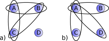
Figure 2: Illustration of the two other possible sets of three two-body marginals: a) a set of marginals, which clearly does not determine the global state, as $\rho_{D}$ is not fixed. b) a set of marginals to which our proof does not apply. Nevertheless, we have numerical evidence that these marginals still determine the state uniquely for qubits.

States that are not UDP. As the proof above is valid for generic states only, it is natural to ask whether there are special four-particle states that are not UDP. This is indeed the case. In the following, we give an incomplete list of undetermined four-particle qubit states. Note that if any two states $\ket{\psi}$ and $\ket{\phi}$ share the same two-body marginals, then also all local unitary equivalent states $\ket{\psi}^{\prime}=U_{A}\otimes U_{B}\otimes U_{C}\otimes U_{D}\ket{\psi}$ and $\ket{\phi}^{\prime}=U_{A}\otimes U_{B}\otimes U_{C}\otimes U_{D}\ket{\phi}$ share the same marginals. Thus, we restrict ourselves to states $\ket{\psi}=\sum\alpha_{ijkl}\ket{ijkl}$ of the standard form introduced in Ref. (Carteret, Higuchi, and Sudbery, 2000), where

$$\alpha_{0000},\alpha_{0001},\alpha_{0010},\alpha_{0100},\alpha_{1000} \in \mathbb{R}\>,$$

$$\alpha_{0111},\alpha_{1011},\alpha_{1101},\alpha_{1110} = 0$$ (38)

and all other coefficients being complex. In the following list, the states are always assumed to be normalized. To shorten the notation, we make use of the $W$ state

$$\ket{W_{4}}=\frac{1}{2}(\ket{0001}+\ket{0010}+\ket{0100}+\ket{1000})$$

and of the Dicke state

$$\ket{D_{2}^{4}} = \frac{1}{\sqrt{6}}(\ket{0011}+\ket{0101}+\ket{1001}$$

$$\hphantom{\frac{1}{\sqrt{6}}(}+\ket{0110}+\ket{1010}+\ket{1100}).$$

Due to the standard form, we have in the following $a,b\in\mathbb{R}$, while $r,s\in\mathbb{C}$. The claimed properties of the states can directly be computed.

• For fixed $a,b$ and $s$, the family

  $$\ket{\psi}=a\ket{0000}+b\ket{W_{4}}+se^{i\varphi}\ket{1111}$$ (39)

  shares the same two-body marginals for all values of $\varphi$.

• For the same state with $a=0,b=\frac{2}{\sqrt{6}}$ and $s=\frac{1}{\sqrt{3}}$,

  $$\ket{\phi}=\frac{1}{2}\ket{0000}+\frac{1}{\sqrt{2}}e^{i\varphi}\ket{D_{2}^{4}}-\frac{1}{2}e^{2i\varphi}\ket{1111}$$ (40)

  shares the same marginals for all values of $\varphi$.

• For every state

  $$\ket{\psi}=a\ket{0000}+r\ket{D_{2}^{4}}+s\ket{1111},$$ (41)

  the state

  $$\ket{\phi}=a\ket{0000}+re^{i\varphi_{r}}\ket{D_{2}^{4}}+se^{i\varphi_{s}}\ket{1111}$$ (42)

  shares the same marginals if $\overline{r}se^{i\varphi_{s}}=are^{i\varphi_{r}}(1-e^{i\varphi_{r}})+\overline{r}se^{i\varphi_{r}}$, which is feasible for e.g., $a=0$.

All of our examples are superpositions of Dicke states and generalized GHZ states. By a local unitary operation, these examples also include the Dicke state with three excitations. The examples prove that Theorem 3 does not hold for all four-particle states, but only for generic states.

Discussion. We have shown that generic four-qudit pure states are uniquely determined among pure states by three of their six different marginals of two parties. Interestingly, from this it follows that pure states of an arbitrary number of qudits are determined by certain subsets of their marginals having size $n-2$. The proof required two marginals of distinct systems to be equal, for instance $\rho_{\text{AB}}$ and $\rho_{\text{CD}}$, in order to fix the Schmidt decomposition of the compatible state. However, there are two other sets of three two-body marginals, illustrated in Fig. 2. The first one, namely knowledge of $\rho_{\text{AB}}$, $\rho_{\text{AC}}$ and $\rho_{\text{BC}}$, is certainly not sufficient to fix the state, as we do not have any knowledge of particle $D$ in this case: Every product state $\rho_{\text{ABC}}\otimes\rho_{\text{D}}$ with arbitrary state $\rho_{\text{D}}$ is compatible. The situation for the second configuration, namely knowledge of the three marginals $\rho_{\text{AB}}$, $\rho_{\text{AC}}$ and $\rho_{\text{AD}}$, is not that clear. In a numerical survey testing random four-qubit states, we could not find pairs of different pure states which coincide on these marginals. Thus, we conjecture that any marginal configuration involving all four parties determines generic states. In any case, knowledge of any set of four two-body marginals fixes the state, as there are always two marginals of distinct particle pairs present in these sets.

The question remains which pure four-qubit states are also uniquely determined among all mixed states by their two-body marginals. The results from Ref. (Jones and Linden, 2005) suggest that generic states are not UDA, and Ref. (Huber and Gühne, 2016) shows that for the case of four qutrits and knowledge of all marginals, as well as for four qubits and the special marginal configuration of Fig. 1 (b), generic states are not UDA. On the other hand, in the same reference, a numerical procedure indicated that for generic pure four-qubit states the compatible mixed states (having the same marginals) are never of full rank. Clarifying this situation is an interesting problem for further research.

Acknowledgments. This work was supported by the Swiss National Science Foundation (Doc.Mobility Grant 165024), the COST Action MP1209, the DFG, and the ERC (Consolidator Grant No. 683107/TempoQ).

References

• Tóth et al. (2009) G. Tóth, C. Knapp, O. Gühne,  and H. J. Briegel, Phys. Rev. A 79, 042334 (2009).
• Würflinger et al. (2012) L. E. Würflinger, J.-D. Bancal, A. Acín, N. Gisin,  and T. Vértesi, Phys. Rev. A 86, 032117 (2012).
• Walter et al. (2013) M. Walter, B. Doran, D. Gross,  and M. Christandl, Science 340, 1205 (2013).
• Miklin, Moroder, and Gühne (2016) N. Miklin, T. Moroder,  and O. Gühne, Phys. Rev. A 93, 020104 (2016).
• Coleman (1963) A. J. Coleman, Rev. Mod. Phys. 35, 668 (1963).
• (6) A. Klyachko,  quant-ph/0409113 .
• Sawicki, Walter, and Kus (2013) A. Sawicki, M. Walter,  and M. Kus, J. Phys. A: Math. Theor. 46, 055304 (2013).
• (8) C. Schilling, C. L. Benavides-Riveros,  and P. Vrana,  arxiv:1703.01612 .
• Zhou (2009) D. L. Zhou, Phys. Rev. A 80, 022113 (2009).
• Huber and Gühne (2016) F. Huber and O. Gühne, Phys. Rev. Lett. 117, 010403 (2016).
• Linden, Popescu, and Wootters (2002) N. Linden, S. Popescu,  and W. Wootters, Phys. Rev. Lett. 89, 207901 (2002).
• Diósi (2004) L. Diósi, Phys. Rev. A 70, 010302 (2004).
• Jones and Linden (2005) N. S. Jones and N. Linden, Phys. Rev. A 71, 012324 (2005).
• Chen et al. (2013) J. Chen, H. Dawkins, Z. Ji, N. Johnston, D. Kribs, F. Shultz,  and B. Zeng, Phys. Rev. A 88, 012109 (2013).
• Xin et al. (2017) T. Xin, D. Lu, J. Klassen, N. Yu, Z. Ji, J. Chen, X. Ma, G. Long, B. Zeng,  and R. Laflamme, Phys. Rev. Lett. 118, 020401 (2017).
• Scott and Caves (2003) A. J. Scott and C. M. Caves, Journal of Phys. A: Math. and Gen. 36, 9553 (2003).
• Lloyd and Pagels (1988) S. Lloyd and H. Pagels, Ann. Phys. 188, 186 (1988).
• Carteret, Higuchi, and Sudbery (2000) H. Carteret, A. Higuchi,  and A. Sudbery, J. Math. Phys. 41, 7932 (2000).