Sensitivity of Love and quasi-Rayleigh waves to model parameters

D.R. Dalton111 Department of Earth Sciences, Memorial University of Newfoundland, Canada, dalton.nfld@gmail.com , M.A. Slawinski222 Department of Earth Sciences, Memorial University of Newfoundland, Canada, mslawins@mac.com , P. Stachura333 Faculty of Applied Informatics and Mathematics, SGGW, Poland, piotr_stachura1@sggw.pl , T. Stanoev444 Department of Earth Sciences, Memorial University of Newfoundland, Canada, theodore.stanoev@gmail.com
(March 31, 2017)
Abstract

We examine the sensitivity of the Love and the quasi-Rayleigh waves to model parameters. Both waves are guided waves that propagate in the same model of an elastic layer above an elastic halfspace. We study their dispersion curves without any simplifying assumptions, beyond the standard approach of elasticity theory in isotropic media. We examine the sensitivity of both waves to elasticity parameters, frequency and layer thickness, for varying frequency and different modes. In the case of Love waves, we derive and plot the absolute value of a dimensionless sensitivity coefficient in terms of partial derivatives, and perform an analysis to find the optimum frequency for determining the layer thickness. For a coherency of the background information, we briefly review the Love-wave dispersion relation and provide details of the less common derivation of the quasi-Rayleigh relation in an appendix. We compare that derivation to past results in the literature, finding certain discrepancies among them.

1 Introduction

In this paper, we examine the sensitivity of the Love and quasi-Rayleigh waves to model parameters. This study provides insight into the reliability of inferences of model properties from data. Herein, sensitivity refers to relations between the wave properties and model parameters in the context of dispersion relations. It does not refer to a misfit between a model and experimental data.

Both waves propagate within an elastic isotropic layer over an elastic isotropic halfspace. This provides a redundancy of information, since both waves are described in terms of the same model parameters. To examine the sensitivity—given the elasticity parameters, mass densities and the thickness of the layer, as well as the frequency of the signal—we study expressions for the speeds of the waves that correspond to different modes for either wave. In general, each wave has an infinite number of modes and each mode propagates with a different speed. However, for a given frequency, there is a finite number of modes, and hence, speeds.

On the surface, the two waves exhibit displacements that are perpendicular to each other. The displacements of the Love wave are in the horizontal plane and perpendicular to the direction of propagation. The displacements of the quasi-Rayleigh wave are in the vertical plane, and—on the surface—are parallel to the direction of propagation. Thus, different speeds and displacement directions render these waves and their modes empirically distinguishable.

The quasi-Rayleigh wave shares many similarities with the classical Rayleigh wave, but is not restricted to the halfspace alone. In literature, the quasi-Rayleigh wave has been also referred to as Rayleigh-type wave, Rayleigh-like wave, generalized Rayleigh wave, Rayleigh-Lamb wave and Rayleigh wave in inhomogeneous media.

Seismological information, such as wave speeds measured on the surface, allow us to infer properties of the subsurface. Herein, to gain insight into such an inverse problem, we examine the sensitivity of the forward one. Wave speeds corresponding to different modes of either wave exhibit different sensitivities to model parameters.

Motivated by the accuracy of modern seismic measurements and availability of computational tools, we study the Love and quasi-Rayleigh dispersion curves without any simplifying assumptions, beyond the standard approach of elasticity theory in isotropic media.

The presented concept of studying sensitivities exhibits certain similarities to the recent work of Lucena and Taioli [1], but with a different approach and scope. The novelty of this study consists of an analysis of the sensitivity of the dispersion relation to elasticity parameters and layer thickness for both Love and quasi-Rayleigh waves for varying frequencies and different modes. Furthermore, we formulate a dimensionless sensitivity coefficient analysis from which we obtain the optimum frequency of Love waves for determining layer thickness.

We begin this paper by examining Love waves and proceed to quasi-Rayleigh waves. In either case, we discuss the sensitivity of the dispersion relations to elasticity parameters and layer thickness for varying frequencies and different modes. We highlight the sensitivity results in Section 4.2 and suggest further research directions in Section 5. This paper contains three appendices, which consist, respectively, of the derivation of the quasi-Rayleigh dispersion relation, calculations of its determinant and a comparison to literature results.

2 Love waves

2.1 Material properties

We wish to examine the sensitivity of guided SH𝑆𝐻SH waves to model parameters. For this purpose, we consider an elastic layer with mass density, ρusuperscript𝜌𝑢\rho^{u} , elasticity parameter, C44usuperscriptsubscript𝐶44𝑢C_{44}^{u} , and hence, S𝑆S-wave propagation speed, βu=C44u/ρusuperscript𝛽𝑢superscriptsubscript𝐶44𝑢superscript𝜌𝑢\beta^{u}=\sqrt{C_{44}^{u}/\rho^{u}} . Also, we consider an elastic halfspace with ρdsuperscript𝜌𝑑\rho^{d} , C44dsuperscriptsubscript𝐶44𝑑C_{44}^{d} and βd=C44d/ρdsuperscript𝛽𝑑superscriptsubscript𝐶44𝑑superscript𝜌𝑑\beta^{d}=\sqrt{C_{44}^{d}/\rho^{d}}. We set the coordinate system in such a manner that the surface is at x3=0subscript𝑥30x_{3}=0 and the interface is at x3=Zsubscript𝑥3𝑍x_{3}=Z , with the x3subscript𝑥3x_{3}-axis positive downwards.

For details of the derivation of the Love wave dispersion relation, see, for instance, Slawinski [2, Chapter 6] and references therein. The dispersion relation for Love waves can be written as

tan(ω1(βu)21v2Z)=C44d1v21(βd)2C44u1(βu)21v2.𝜔1superscriptsuperscript𝛽𝑢21superscriptsubscript𝑣2𝑍superscriptsubscript𝐶44𝑑1superscriptsubscript𝑣21superscriptsuperscript𝛽𝑑2superscriptsubscript𝐶44𝑢1superscriptsuperscript𝛽𝑢21superscriptsubscript𝑣2\tan\left(\omega\sqrt{\frac{1}{(\beta^{u})^{2}}-\frac{1}{v_{\ell}^{2}}}\,Z\right)=\frac{C_{44}^{d}\,\sqrt{\dfrac{\mathstrut 1}{v_{\ell}^{2}}-\dfrac{1}{(\beta^{d})^{2}}}}{C_{44}^{u}\,\sqrt{\mathstrut\dfrac{\mathstrut 1}{(\beta^{u})^{2}}-\dfrac{1}{v_{\ell}^{2}}}}\,. (1)

To plot expression (1), we rewrite it as an expression equal to zero, where

D=2(C44u(vβu)21sin(ωZβu1(βuv)2)C44d1(vβd)2cos(ωZβu1(βuv)2))=0.subscriptD2superscriptsubscript𝐶44𝑢superscriptsubscript𝑣superscript𝛽𝑢21𝜔𝑍superscript𝛽𝑢1superscriptsuperscript𝛽𝑢subscript𝑣2superscriptsubscript𝐶44𝑑1superscriptsubscript𝑣superscript𝛽𝑑2𝜔𝑍superscript𝛽𝑢1superscriptsuperscript𝛽𝑢subscript𝑣20\mathrm{D}_{\ell}=2\left(C_{44}^{u}\sqrt{\left(\frac{v_{\ell}}{\beta^{u}}\right)^{\!\!2}-1}\,\sin\left(\frac{\omega Z}{\beta^{u}}\sqrt{1-\left(\frac{\beta^{u}}{v_{\ell}}\right)^{\!\!2}}\,\right)-C_{44}^{d}\sqrt{1-\left(\frac{v_{\ell}}{\beta^{d}}\right)^{\!\!2}}\,\cos\left(\frac{\omega Z}{\beta^{u}}\sqrt{1-\left(\frac{\beta^{u}}{v_{\ell}}\right)^{\!\!2}}\,\right)\right)=0\,. (2)

We plot expression (2) within a model in which we set the layer thickness Z=500m𝑍500mZ=500~{}{\rm m} , the two elasticity parameters, C44u=0.88×10¹⁰N/m2superscriptsubscript𝐶44𝑢0.88superscript1010Nsuperscriptm2C_{44}^{u}=0.88\times 10^{10}~{}{\rm N}/{\rm m}^{2} and C44d=4.16×10¹⁰N/m2superscriptsubscript𝐶44𝑑4.16superscript1010Nsuperscriptm2C_{44}^{d}=4.16\times 10^{10}~{}{\rm N}/{\rm m}^{2} , and mass densities, ρu=2200kg/m3superscript𝜌𝑢2200kgsuperscriptm3\rho^{u}=2200~{}{\rm kg}/{\rm m}^{3} and ρd=2600kg/m3superscript𝜌𝑑2600kgsuperscriptm3\rho^{d}=2600~{}{\rm kg}/{\rm m}^{3} . It follows that the S𝑆S-wave propagation speeds in the layer and the halfspace are βu=2000m/ssuperscript𝛽𝑢2000ms\beta^{u}=2000~{}{\rm m}/{\rm s} and βd=4000m/ssuperscript𝛽𝑑4000ms\beta^{d}=4000~{}{\rm m}/{\rm s} , respectively. Such a model could represent a sandstone layer over a granite halfspace.

Refer to caption
Refer to caption
Figure 1: DsubscriptD\mathrm{D}_{\ell} , defined in expression (2), as a function of speed, vsubscript𝑣v_{\ell} . On the left, for ω=60s1𝜔60superscripts1\omega=60~{}{\rm s}^{-1} , there are five roots: v=2010.7m/ssubscript𝑣2010.7ms{v_{\ell}=2010.7~{}{\rm m}/{\rm s}} , v=2102.76m/ssubscript𝑣2102.76msv_{\ell}=2102.76~{}{\rm m}/{\rm s} , v=2330.44m/ssubscript𝑣2330.44msv_{\ell}=2330.44~{}{\rm m}/{\rm s} , v=2853.13m/ssubscript𝑣2853.13msv_{\ell}=2853.13~{}{\rm m}/{\rm s} and v=3958.53m/ssubscript𝑣3958.53msv_{\ell}=3958.53~{}{\rm m}/{\rm s} . On the right, for ω=15s1𝜔15superscripts1\omega=15~{}{\rm s}^{-1} , there are two roots: v=2172.48m/ssubscript𝑣2172.48msv_{\ell}=2172.48~{}{\rm m}/{\rm s} and v=3997.01m/ssubscript𝑣3997.01msv_{\ell}=3997.01~{}{\rm m}/{\rm s} . The values on the vertical axes are to be multiplied by 1010superscript101010^{10} .
Refer to caption
Figure 2: The Love-wave dispersion curves, D=0subscriptD0\mathrm{D}_{\ell}=0 , defined in expression (2), as a function of speed, vsubscript𝑣v_{\ell} , and frequency, ω𝜔\omega .

Examining the left and right plots of Figure 1, as well as the dispersion curves in Figure 2, we see that, for high frequency, ω=60s1𝜔60superscripts1\omega=60~{}{\rm s}^{-1} , the speed of the fundamental mode of the Love wave, v=2011m/ssubscript𝑣2011msv_{\ell}=2011~{}{\rm m}/{\rm s} , approaches βusuperscript𝛽𝑢\beta^{u} , from above. The values of vsubscript𝑣v_{\ell} are computed numerically. This result is in agreement with Udías [3, p. 196], and with the general theory of Love waves.

2.2 Sensitivity of dispersion relation

We wish to examine effects of elasticity parameters and layer thickness on the dispersion relation, for various frequencies and different modes. To do so, we examine effects of these quantities on the value of DsubscriptD\mathrm{D}_{\ell} , defined in expression (2). Specifically, we examine DsubscriptD\mathrm{D}_{\ell} as a function of C44dsuperscriptsubscript𝐶44𝑑C_{44}^{d} and C44usuperscriptsubscript𝐶44𝑢C_{44}^{u} , for two distinct frequencies and for fixed values of vsubscript𝑣v_{\ell} , which correspond to particular modes.

In the contour maps of Figures 36, the sensitivity of the dispersion relation is illustrated by the slope of the zero contour line, where a vertical line implies no sensitivity to the parameter on the vertical axis and a horizontal line implies no sensitivity to the parameter on the horizontal axis. In other words, a parallel line does not restrict the values on the corresponding axis. The zero contour line is the combination of elasticity parameters that result in a solution, D=0subscript𝐷0D_{\ell}=0. Hence, from a vertical line we infer that the horizontal axis parameter is fixed but the vertical axis parameter is not constrained. Our approach differs from the approach of Lucena and Taioli [1], who examine the response of the dispersion curves to shifts in parameter values.
Refer to caption
Refer to caption
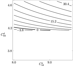
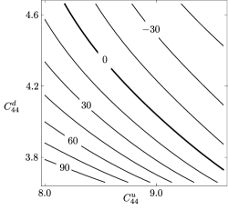
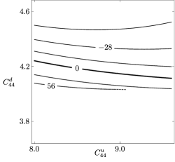
Figure 3: D/109subscriptDsuperscript109\mathrm{D}_{\ell}/10^{9} , defined in expression (2), as a function of the elasticity parameters, C44usuperscriptsubscript𝐶44𝑢C_{44}^{u} and C44dsuperscriptsubscript𝐶44𝑑C_{44}^{d} , for ω=60s1𝜔60superscripts1\omega=60~{}{\rm s}^{-1} and v=3958.53m/ssubscript𝑣3958.53msv_{\ell}=3958.53~{}{\rm m}/{\rm s} , on the left, and for ω=15s1𝜔15superscripts1\omega=15~{}{\rm s}^{-1} and v=3997.01m/ssubscript𝑣3997.01msv_{\ell}=3997.01~{}{\rm m}/{\rm s} , on the right. The values on the horizontal and vertical axes are to be multiplied by 109superscript10910^{9} and 1010superscript101010^{10} , respectively. Both plots demonstrate sensitivity to C44usuperscriptsubscript𝐶44𝑢C_{44}^{u} and C44dsuperscriptsubscript𝐶44𝑑C_{44}^{d} but the right plot, for lower frequency, demonstrates a greater sensitivity to C44dsuperscriptsubscript𝐶44𝑑C_{44}^{d} .
Refer to caption
Refer to caption
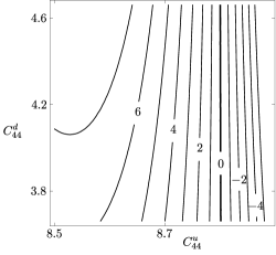
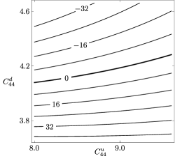
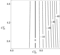
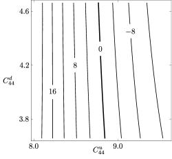
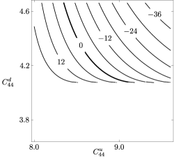
Figure 4: D/1010subscriptDsuperscript1010\mathrm{D}_{\ell}/10^{10} , defined in expression (2), as a function of the elasticity parameters, C44usuperscriptsubscript𝐶44𝑢C_{44}^{u} and C44dsuperscriptsubscript𝐶44𝑑C_{44}^{d} , where ω=60s1𝜔60superscripts1\omega=60~{}{\rm s}^{-1} and v=2010.7m/ssubscript𝑣2010.7msv_{\ell}=2010.7~{}{\rm m}/{\rm s} , and where ω=15s1𝜔15superscripts1\omega=15~{}{\rm s}^{-1} and v=2172.48m/ssubscript𝑣2172.48msv_{\ell}=2172.48~{}{\rm m}/{\rm s} , for left and right, respectively. The values on the horizontal and vertical axes are to be multiplied by 109superscript10910^{9} and 1010superscript101010^{10} , respectively. We see from the zero contours, which are near vertical, that there is sensitivity to C44usuperscriptsubscript𝐶44𝑢C_{44}^{u} and not to C44dsuperscriptsubscript𝐶44𝑑C_{44}^{d} , and this contrast is slightly more pronounced for the higher frequency case.

Let us examine the numerical solutions of speed for the Love wave dispersion relation for the high-frequency and low-frequency cases. We use these solutions to investigate the relative sensitivities of Love waves to the elasticity parameters in the upper layer and in the lower halfspace, as well as to the elasticity parameter in the upper layer and to the layer thickness.

We begin by considering the layer and halfspace elasticity parameters. For the high-speed case, we consider the fifth root of the left plot of Figure 1, which is v=3959m/ssubscript𝑣3959msv_{\ell}=3959~{}{\rm m}/{\rm s} , and the second root of the right plot of Figure 1, which is v=3997m/ssubscript𝑣3997msv_{\ell}=3997~{}{\rm m}/{\rm s} . The left and right plots of Figure 3 are the corresponding contour plots of D/109subscript𝐷superscript109D_{\ell}/10^{9} with varying C44usuperscriptsubscript𝐶44𝑢C_{44}^{u} and C44dsuperscriptsubscript𝐶44𝑑C_{44}^{d} . In both cases, Dsubscript𝐷D_{\ell} is sensitive to variations in both C44usuperscriptsubscript𝐶44𝑢C_{44}^{u} and C44dsuperscriptsubscript𝐶44𝑑C_{44}^{d} . However, the right plot of Figure 3 indicates a greater sensitivity to C44dsuperscriptsubscript𝐶44𝑑C_{44}^{d} for the lower frequency, which is tantamount to longer wavelength.

For the low-speed case, we observe different sensitivities. Let us examine the first root of the left plot of Figure 1, which is v=2005m/ssubscript𝑣2005msv_{\ell}=2005~{}{\rm m}/{\rm s} , and the first root of the right plot of Figure 1, which is v=2172m/ssubscript𝑣2172msv_{\ell}=2172~{}{\rm m}/{\rm s} . Following the corresponding plots in Figure 4, we see that there are near vertical lines at C44u=0.88×10¹⁰superscriptsubscript𝐶44𝑢0.88superscript1010C_{44}^{u}=0.88\times 10^{10} . This indicates a sensitivity toward C44usuperscriptsubscript𝐶44𝑢C_{44}^{u} but not toward C44dsuperscriptsubscript𝐶44𝑑C_{44}^{d} , and we observe that it is more pronounced for the left plot. Thus, for a given wavelength, a solution whose speed is closer to βusuperscript𝛽𝑢\beta^{u} is less sensitive to C44dsuperscriptsubscript𝐶44𝑑C_{44}^{d} than a solution with greater speed.

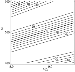
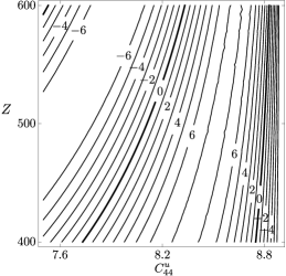
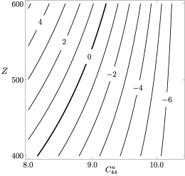
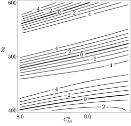
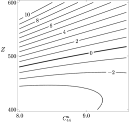
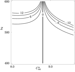
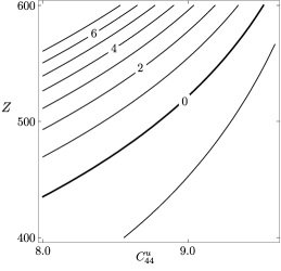
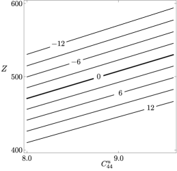
Next, we consider the layer elasticity parameter and layer thickness. Using the high-speed roots of expression (2), we observe sensitivity to both C44usuperscriptsubscript𝐶44𝑢C_{44}^{u} and Z𝑍Z , in the high-frequency and low-frequency cases, which are depicted in Figure 5. Using low-speed roots in Figure 6, we see that there is less sensitivity to Z𝑍Z for higher frequencies than lower frequencies. Note that, in the left plot of Figure 5, the groups of contours in the upper left and lower right are due to the periodicity of Dsubscript𝐷D_{\ell} in Z𝑍Z , as discussed is section 2.3, below.
Refer to caption
Refer to caption
Figure 5: D/109subscriptDsuperscript109\mathrm{D}_{\ell}/10^{9} , defined in expression (2), as a function of C44usuperscriptsubscript𝐶44𝑢C_{44}^{u} and Z𝑍Z , for ω=60s1𝜔60superscripts1\omega=60~{}{\rm s}^{-1} and v=3958.53m/ssubscript𝑣3958.53msv_{\ell}=3958.53~{}{\rm m}/{\rm s} , on the left, and for ω=15s1𝜔15superscripts1\omega=15~{}{\rm s}^{-1} and v=3997.01m/ssubscript𝑣3997.01msv_{\ell}=3997.01~{}{\rm m}/{\rm s} , on the right. The values on the horizontal axis are to be multiplied by 109superscript10910^{9} . In each case, there is sensitivity to both C44usuperscriptsubscript𝐶44𝑢C_{44}^{u} and Z𝑍Z .
Refer to caption
Refer to caption
Figure 6: D/1010subscriptDsuperscript1010\mathrm{D}_{\ell}/10^{10} , defined in expression (2), as a function of C44usuperscriptsubscript𝐶44𝑢C_{44}^{u} and Z𝑍Z , where ω=60s1𝜔60superscripts1\omega=60~{}{\rm s}^{-1} and v=2010.7m/ssubscript𝑣2010.7msv_{\ell}=2010.7~{}{\rm m}/{\rm s} , and where ω=15s1𝜔15superscripts1\omega=15~{}{\rm s}^{-1} and v=2172.48m/ssubscript𝑣2172.48msv_{\ell}=2172.48~{}{\rm m}/{\rm s} , for left and right, respectively. In the left plot, the zero contour of interest is the near-vertical one on the right side of the plot, near the maximum C44usuperscriptsubscript𝐶44𝑢C_{44}^{u} . The values on the horizontal axis are to be multiplied by 109superscript10910^{9} . In each case, there is sensitivity to both C44usuperscriptsubscript𝐶44𝑢C_{44}^{u} and Z𝑍Z , but the higher frequency case has less sensitivity to Z𝑍Z .

Additionally, the two plots of Figure 6, along with the left plot of Figure 4, approach a maximum value of C44usuperscriptsubscript𝐶44𝑢C_{44}^{u} , whereas the two plots of Figure 5 do not. To understand this behaviour, we recall that, as a consequence of the allowable range of Love-wave speeds, βu<v<βdsuperscript𝛽𝑢subscript𝑣superscript𝛽𝑑\beta^{u}<v_{\ell}<\beta^{d} , there is a maximum value of C44usuperscriptsubscript𝐶44𝑢C_{44}^{u} whose value is v2ρusuperscriptsubscript𝑣2superscript𝜌𝑢v_{\ell}^{2}\rho^{u} .

2.3 Love wave as superposition of SH𝑆𝐻SH waves

The ridge and valley behaviour, shown in Figures 5 and 6, can be explained by examining the nonzero component of the displacement,

u2u(x1,x3,t)=C1exp(ικsux3)exp[ι(κx1ωt)]+C2exp(ικsux3)exp[ι(κx1ωt)],superscriptsubscript𝑢2𝑢subscript𝑥1subscript𝑥3𝑡subscript𝐶1𝜄𝜅superscript𝑠𝑢subscript𝑥3𝜄𝜅subscript𝑥1𝜔𝑡subscript𝐶2𝜄𝜅superscript𝑠𝑢subscript𝑥3𝜄𝜅subscript𝑥1𝜔𝑡u_{2}^{u}(x_{1},x_{3},t)=C_{1}\exp{\left(-\iota\kappa s^{u}x_{3}\right)}\exp[\iota(\kappa x_{1}-\omega t)]+C_{2}\exp{\left(\iota\kappa s^{u}x_{3}\right)}\exp[\iota(\kappa x_{1}-\omega t)]\,,

where su:=(v/βu)21assignsuperscript𝑠𝑢superscriptsubscript𝑣superscript𝛽𝑢21s^{u}:=\sqrt{(v_{\ell}/\beta^{u})^{2}-1} . This expression can be interpreted as a superposition of two SH𝑆𝐻SH waves within the elastic layer. Both waves travel obliquely with respect to the surface and interface; one wave travels upwards, the other downwards. Their wave vectors are k¯±:=(κ,0,±κsu)assignsubscript¯𝑘plus-or-minus𝜅0plus-or-minus𝜅superscript𝑠𝑢\overline{k}_{\pm}:=(\kappa,0,\pm\kappa s^{u}) . Thus, since

|k¯±|=κ2+(κsu)2,subscript¯𝑘plus-or-minussuperscript𝜅2superscript𝜅superscript𝑠𝑢2|\overline{k}_{\pm}|=\sqrt{\kappa^{2}+(\kappa\,s^{u})^{2}}\,,

we have

|k¯±|=κ1+(su)2=κvβu,subscript¯𝑘plus-or-minus𝜅1superscriptsuperscript𝑠𝑢2𝜅subscript𝑣superscript𝛽𝑢|\overline{k}_{\pm}|=\kappa\sqrt{1+(s^{u})^{2}}=\kappa\,\frac{v_{\ell}}{\beta^{u}}\,,

where

βuv=κ|k±|=sinθ,superscript𝛽𝑢subscript𝑣𝜅subscript𝑘plus-or-minus𝜃\frac{\beta^{u}}{v_{\ell}}=\frac{\kappa}{|k_{\pm}|}=\sin\theta\,,

with θ𝜃\theta representing for the angle between k¯±subscript¯𝑘plus-or-minus\overline{k}_{\pm} and the x3subscript𝑥3x_{3}-axis. Thus, θ𝜃\theta is the angle between the x3subscript𝑥3x_{3}-axis and a wavefront normal, which implies that it is the propagation direction of a wavefront. Hence, for the case where vsubscript𝑣v_{\ell} is only slightly larger than βusuperscript𝛽𝑢\beta^{u} , it follows that both the upgoing and downgoing SH𝑆𝐻SH waves propagate nearly horizontally. In other words, their propagation directions are nearly parallel to the interface. In such a case, the resulting Love wave is less sensitive to the material properties below the interface than for the case of βu/v1much-less-thansuperscript𝛽𝑢subscript𝑣1\beta^{u}/v_{\ell}\ll 1 .

Depending on the propagation direction, θ𝜃\theta , of the SH𝑆𝐻SH waves, there is a distinction in the sensitivity to the material properties of the halfspace. This distinction is more pronounced for short wavelengths, in comparison with the layer thickness. For any angle, the longer the wavelength the more sensitivity of the wave to material properties below the interface, and thus the distinction—as a function of the propagation direction—is diminished.

Also, the superposition helps us understand the requirement of βu<v<βdsuperscript𝛽𝑢subscript𝑣superscript𝛽𝑑\beta^{u}<v_{\ell}<\beta^{d} . The lower limit, which we can write as sinθ=βu/βu=1𝜃superscript𝛽𝑢superscript𝛽𝑢1\sin\theta=\beta^{u}/\beta^{u}=1 , corresponds to waves that propagate along the x1subscript𝑥1x_{1}-axis, and hence, do not exhibit any interference associated with the presence of the horizontal surface or interface. Formally, the lower limit is required by the real value of the sine function.

The upper limit is introduced to ensure an exponential amplitude decay in the halfspace. Herein, we can write the upper limit as sinθ=βu/βd𝜃superscript𝛽𝑢superscript𝛽𝑑\sin\theta=\beta^{u}/\beta^{d} , which—in general—implies that the SH𝑆𝐻SH waves propagate obliquely. In the extreme case, if βdsuperscript𝛽𝑑\beta^{d}\to\infty , the waves propagate vertically. Also, this case is tantamount to total internal reflection, since it corresponds to a rigid halfspace, C44dsuperscriptsubscript𝐶44𝑑C_{44}^{d}\to\infty ; such a case is discussed by Slawinski [2, Section 6.3.1].

2.4 Optimum frequency for layer-thickness determination

In this section, we search for the best frequency for inferring the depth of the interface. Given the values of the elasticity parameters and layer thickness, for a specific frequency, we deduce the corresponding propagation speed. For a given mode, this speed depends on Z𝑍Z , which means that Z𝑍Z is a function of speed. Since, experimentally, the speed is measured with only finite accuracy, we inherit that finite accuracy for any inference of the value of Z𝑍Z .

As a measure of sensitivity of Z𝑍Z to errors in speed, we take the derivative, dZ/dvd𝑍d𝑣{\rm d}Z/{\rm d}v , or, more precisely, its ratio to Z𝑍Z , namely,

A~:=1ZdZdv.assign~𝐴1𝑍d𝑍d𝑣\tilde{A}:=\frac{1}{Z}\frac{{\rm d}Z}{{\rm d}v}\,. (3)

For convenience, we write relation (2) using dimensionless quantities. If we let

α:=C44dρuC44uρd=βdβu>1,E:=C44dρdC44uρu,θ:=vβu,ν:=ωZβu,formulae-sequenceassign𝛼superscriptsubscript𝐶44𝑑superscript𝜌𝑢superscriptsubscript𝐶44𝑢superscript𝜌𝑑superscript𝛽𝑑superscript𝛽𝑢1formulae-sequenceassign𝐸superscriptsubscript𝐶44𝑑superscript𝜌𝑑superscriptsubscript𝐶44𝑢superscript𝜌𝑢formulae-sequenceassign𝜃subscript𝑣superscript𝛽𝑢assign𝜈𝜔𝑍superscript𝛽𝑢\alpha:=\sqrt{\frac{C_{44}^{d}\rho^{u}}{C_{44}^{u}\rho^{d}}}=\frac{\beta^{d}}{\beta^{u}}>1\,,\quad E:=\sqrt{\frac{C_{44}^{d}\rho^{d}}{C_{44}^{u}\rho^{u}}}\,,\quad\theta:=\frac{v_{\ell}}{\beta^{u}}\,,\quad\nu:=\frac{\omega Z}{\beta^{u}}\,, (4)

then relation (2) becomes

F(ν,θ):=θ21sin(ν11θ2)Eα2θ2cos(ν11θ2)=0,assign𝐹𝜈𝜃superscript𝜃21𝜈11superscript𝜃2𝐸superscript𝛼2superscript𝜃2𝜈11superscript𝜃20F(\nu,\theta):=\sqrt{\theta^{2}-1}\sin\left(\nu\sqrt{1-\frac{1}{\theta^{2}}}\right)-E\sqrt{\alpha^{2}-\theta^{2}}\cos\left(\nu\sqrt{1-\frac{1}{\theta^{2}}}\right)=0\,, (5)

where 1<θ<α1𝜃𝛼1<\theta<\alpha and ν>0𝜈0\nu>0 . Using the Implicit Function Theorem, the following properties are shown.

  • \circ

    F(ν,θ)=0𝐹𝜈𝜃0F(\nu,\theta)=0 defines locally θ𝜃\theta as a function of ν𝜈\nu , and, reciprocally, ν𝜈\nu as a function of θ𝜃\theta .

  • \circ

    F(ν,θ)=0𝐹𝜈𝜃0F(\nu,\theta)=0 has a solution 1<θ<α1𝜃𝛼1<\theta<\alpha for any ν>0𝜈0\nu>0 . The smallest such solution is the fundamental mode; it is a smooth and strictly decreasing function of ν𝜈\nu; it is invertible and defines ν𝜈\nu as a function of θ𝜃\theta .

  • \circ

    Higher modes start at νk>0,k=1,2,,formulae-sequencesubscript𝜈𝑘0𝑘12\nu_{k}>0\,,\,k=1,2,\dots, and define θ𝜃\theta as strictly decreasing functions of ν𝜈\nu .

The Implicit Function Theorem is also used in a related study by Novotný [4] except his dispersion relation remains in its tangent form.

Following the definition of A~~𝐴\tilde{A} , in expression (3), it is convenient to measure speed in units of βusuperscript𝛽𝑢\beta^{u} so that θ𝜃\theta is used instead of v𝑣v . Thus, we define the dimensionless coefficient as

A:=1ZdZdθ.assign𝐴1𝑍d𝑍d𝜃A:=\frac{1}{Z}\frac{{\rm d}Z}{{\rm d}\theta}\,. (6)

Z(θ)𝑍𝜃Z(\theta) , which appears in definition (6), is given by

Z(θ):=βuων(θ),assign𝑍𝜃superscript𝛽𝑢𝜔𝜈𝜃Z(\theta):=\frac{\beta^{u}}{\omega}\,\nu(\theta)\,, (7)

and ν(θ)𝜈𝜃\nu(\theta) is a mode defined by expression (5). Hence,

A=1νdνdθ=1ν1dθdν,wheredθdν=FνFθ.formulae-sequence𝐴1𝜈d𝜈d𝜃1𝜈1d𝜃d𝜈whered𝜃d𝜈𝐹𝜈𝐹𝜃A=\frac{1}{\nu}\frac{{\rm d}\nu}{{\rm d}\theta}=\frac{1}{\nu}\frac{1}{\frac{{\rm d}\theta}{{\rm d}\nu}}\,,\qquad\mbox{where}\qquad\frac{{\rm d}\theta}{{\rm d}\nu}=-\frac{\frac{\partial F}{\partial\nu}}{\frac{\partial F}{\partial\theta}}\,. (8)

To calculate and plot A(ω)𝐴𝜔A(\omega) , given Z𝑍Z , we calculate ν=(ωZ)/βu𝜈𝜔𝑍superscript𝛽𝑢\nu=(\omega Z)/\beta^{u} , given Z𝑍Z and ω𝜔\omega , and numerically find the minimum solution, θ(ν)𝜃𝜈\theta(\nu) , for F=0𝐹0F=0 .

Calculating the partial derivatives and using

sin(ν11θ2)=Eα2θ2cos(ν11θ2)θ21,𝜈11superscript𝜃2𝐸superscript𝛼2superscript𝜃2𝜈11superscript𝜃2superscript𝜃21\sin\left(\nu\sqrt{1-\frac{1}{\theta^{2}}}\right)=\frac{E\sqrt{\alpha^{2}-\theta^{2}}\cos\left(\nu\sqrt{1-\frac{1}{\theta^{2}}}\right)}{\sqrt{\theta^{2}-1}}\,, (9)

from expression (5), we obtain

A=1ν(α21)Eθ3+E2ν(α2θ2)3/2+ν(θ21)α2θ2θ(θ21)α2θ2(θ21+E2(α2θ2)),𝐴1𝜈superscript𝛼21𝐸superscript𝜃3superscript𝐸2𝜈superscriptsuperscript𝛼2superscript𝜃232𝜈superscript𝜃21superscript𝛼2superscript𝜃2𝜃superscript𝜃21superscript𝛼2superscript𝜃2superscript𝜃21superscript𝐸2superscript𝛼2superscript𝜃2A=-\frac{1}{\nu}\frac{\left(\alpha^{2}-1\right)E\theta^{3}+E^{2}\nu(\alpha^{2}-\theta^{2})^{3/2}+\nu\left(\theta^{2}-1\right)\sqrt{\alpha^{2}-\theta^{2}}}{\theta\left(\theta^{2}-1\right)\sqrt{\alpha^{2}-\theta^{2}}\left(\theta^{2}-1+E^{2}(\alpha^{2}-\theta^{2})\right)}\,, (10)

which is the relative dimensionless sensitivity coefficient.

In Figure 7, we examine the relationship between |A|𝐴|A| and ω𝜔\omega for different layer thicknesses. In the left plot, which is the case of Z=100m𝑍100mZ=100~{}{\rm m} , we see that there is a minimum |A|𝐴|A| at about ω0=30s1subscript𝜔030superscripts1\omega_{0}=30~{}{\rm s}^{-1} . In the right plot, which is the case for Z=500m𝑍500mZ=500~{}{\rm m} , the same minimum |A|𝐴|A| occurs at about ω0=7s1subscript𝜔07superscripts1\omega_{0}=7~{}{\rm s}^{-1} .

Refer to caption
Refer to caption
Figure 7: The absolute value of the relative dimensionless sensitivity coefficient, |A|𝐴|A| , is plotted against ω𝜔\omega , for Z=100m𝑍100mZ=100~{}{\rm m} on the left, and for Z=500m𝑍500mZ=500~{}{\rm m} on the right. Both plots begin at ω=1s1𝜔1superscripts1\omega=1\,{\rm s}^{-1} due to the asymptote at ω=0𝜔0\omega=0 . Due to the different vertical scales, the minimum |A|𝐴|A| on each plot is the same.

We wish to calculate the minimal value of |A|𝐴|A| to find the frequency, ω0subscript𝜔0\omega_{0} , where the layer thickness, Z𝑍Z , is least sensitive to variations in speed. To find that value of |A|𝐴|A| , we solve for dA/dν=0d𝐴d𝜈0{\rm d}A/{\rm d}\nu=0 or, equivalently,

ddν(1A)=ddν(νdθdν)=dθdν+νd2θdν2=θ+νθ′′=0.dd𝜈1𝐴dd𝜈𝜈d𝜃d𝜈d𝜃d𝜈𝜈superscriptd2𝜃dsuperscript𝜈2superscript𝜃𝜈superscript𝜃′′0\frac{{\rm d}}{{\rm d}\nu}\left(\frac{1}{A}\right)=\frac{{\rm d}}{{\rm d}\nu}\left(\nu\frac{{\rm d}\theta}{{\rm d}\nu}\right)=\frac{{\rm d}\theta}{{\rm d}\nu}+\nu\frac{{\rm d}^{2}\theta}{{\rm d}\nu^{2}}=\theta^{\prime}+\nu\theta^{\prime\prime}=0\,. (11)

By differentiating F(ν,θ(ν))=0𝐹𝜈𝜃𝜈0F(\nu,\theta(\nu))=0 twice with respect to ν𝜈\nu , we get

2Fν2+22Fθνθ+2Fθ2(θ)2+Fθθ′′=0,superscript2𝐹superscript𝜈22superscript2𝐹𝜃𝜈superscript𝜃superscript2𝐹superscript𝜃2superscriptsuperscript𝜃2𝐹𝜃superscript𝜃′′0\frac{\partial^{2}F}{\partial\nu^{2}}+2\frac{\partial^{2}F}{\partial\theta\partial\nu}\theta^{\prime}+\frac{\partial^{2}F}{\partial\theta^{2}}(\theta^{\prime})^{2}+\frac{\partial F}{\partial\theta}\theta^{\prime\prime}=0\,,

where prime denotes derivative with respect to ν𝜈\nu . In this manner, θ+νθ′′=0superscript𝜃𝜈superscript𝜃′′0\theta^{\prime}+\nu\theta^{\prime\prime}=0 in expression (11) can be written in terms of F𝐹F as

F2(ν,θ)=22FθνFθ+1ν(Fθ)2+2Fθ2Fν=0,subscript𝐹2𝜈𝜃2superscript2𝐹𝜃𝜈𝐹𝜃1𝜈superscript𝐹𝜃2superscript2𝐹superscript𝜃2𝐹𝜈0F_{2}(\nu,\theta)=-2\frac{\partial^{2}F}{\partial\theta\partial\nu}\frac{\partial F}{\partial\theta}+\frac{1}{\nu}\left(\frac{\partial F}{\partial\theta}\right)^{2}+\frac{\partial^{2}F}{\partial\theta^{2}}\frac{\partial F}{\partial\nu}=0\,, (12)

where we use

2Fν2=1θ2θ2F=0.superscript2𝐹superscript𝜈21superscript𝜃2superscript𝜃2𝐹0\frac{\partial^{2}F}{\partial\nu^{2}}=\frac{1-\theta^{2}}{\theta^{2}}F=0\,.
Refer to caption
Refer to caption
Figure 8: The left plot depicts intersecting zero contours of F(ν,θ)𝐹𝜈𝜃F(\nu,\theta) and F2(ν,θ)subscript𝐹2𝜈𝜃F_{2}(\nu,\theta) , where the curve ascending from (0,1)01(0,1) is the zero contour of F2subscript𝐹2F_{2} . The right plot depicts the optimum frequency ω0subscript𝜔0\omega_{0} plotted versus Z𝑍Z .

Evaluating the partial derivatives and using expression (9), we obtain

F2(ν,θ)subscript𝐹2𝜈𝜃\displaystyle F_{2}(\nu,\theta) =\displaystyle= cos2(νθ21θ)θ5(θ21)2(α2θ2){θ((α21)Eθ3+E2ν(α2θ2)3/2+ν(θ21)α2θ2)2ν\displaystyle\frac{\cos^{2}\left(\frac{\nu\sqrt{\theta^{2}-1}}{\theta}\right)}{\theta^{5}\left(\theta^{2}-1\right)^{2}(\alpha^{2}-\theta^{2})}\left\{\frac{\theta\left(\left(\alpha^{2}-1\right)E\theta^{3}+E^{2}\nu(\alpha^{2}-\theta^{2})^{3/2}+\nu\left(\theta^{2}-1\right)\sqrt{\alpha^{2}-\theta^{2}}\right)^{2}}{\nu}\right.
+\displaystyle+ 1α2θ2[(E2(α2θ2)+θ21)((θ21)(α4Eν2α2θ(ν(θ22)α2θ2\displaystyle\frac{1}{\sqrt{\alpha^{2}-\theta^{2}}}\left[\left(E^{2}(\alpha^{2}-\theta^{2})+\theta^{2}-1\right)\left(\left(\theta^{2}-1\right)\left(\alpha^{4}E\nu^{2}-\alpha^{2}\theta\left(\nu\left(\theta^{2}-2\right)\sqrt{\alpha^{2}-\theta^{2}}\right.\right.\right.\right.
+E(2ν2θθ5+θ3))+νθ3((θ22)α2θ2+Eνθ))E(α2θ2)3/2\displaystyle\quad+\left.\left.E\left(2\nu^{2}\theta-\theta^{5}+\theta^{3}\right)\right)+\nu\theta^{3}\left(\left(\theta^{2}-2\right)\sqrt{\alpha^{2}-\theta^{2}}+E\nu\theta\right)\right)-E(\alpha^{2}-\theta^{2})^{3/2}
×(α2Eν(3θ22)θ+α2θ2(ν2(θ21)+θ4)Eνθ5))]\displaystyle\qquad\times\left.\left.\left(\alpha^{2}E\nu\left(3\theta^{2}-2\right)\theta+\sqrt{\alpha^{2}-\theta^{2}}\left(\nu^{2}\left(\theta^{2}-1\right)+\theta^{4}\right)-E\nu\theta^{5}\right)\right)\right]
\displaystyle- [2θ(E2(α2θ4)+θ41)(α4E2ν+α2(Eθ3α2θ2\displaystyle\left[2\theta\left(E^{2}\left(\alpha^{2}-\theta^{4}\right)+\theta^{4}-1\right)\left(\alpha^{4}E^{2}\nu+\alpha^{2}\left(E\theta^{3}\sqrt{\alpha^{2}-\theta^{2}}\right.\right.\right.
+ν(2E2θ2+θ21))+θ2(Eθα2θ2+(E21)νθ2+ν))]}=0.\displaystyle\quad+\left.\left.\nu\left(-2E^{2}\theta^{2}+\theta^{2}-1\right)\Big{)}+\theta^{2}\left(-E\theta\sqrt{\alpha^{2}-\theta^{2}}+\left(E^{2}-1\right)\nu\theta^{2}+\nu\right)\right)\right]\Bigg{\}}=0\,.

Using the system of equations formed by expressions (5) and (2.4), we obtain ν0subscript𝜈0\nu_{0} for which the absolute value of A𝐴A is minimal for a given mode.

The intersection points of F(ν,θ)𝐹𝜈𝜃F(\nu,\theta) and F2(ν,θ)subscript𝐹2𝜈𝜃F_{2}(\nu,\theta) , on the left plot of Figure 8, correspond to solutions, (ν0,θ0)subscript𝜈0subscript𝜃0(\nu_{0},\theta_{0}) , for the first seven modes of A𝐴A in expression (10). In view of the intrinsic nonlinearity, we estimate the coordinates of the intersection points and use them as starting points in a numerical search. The values of (ν0,θ0)subscript𝜈0subscript𝜃0(\nu_{0},\theta_{0}) , for the first seven modes, are (1.58172,1.53806)1.581721.53806(1.58172,1.53806) , (5.23429,1.68935)5.234291.68935(5.23429,1.68935) , (8.90672,1.74515)8.906721.74515(8.90672,1.74515) , (12.5772,1.7779)12.57721.7779(12.5772,1.7779) , (16.2443,1.80044)16.24431.80044(16.2443,1.80044) , (19.9085,1.81731)19.90851.81731(19.9085,1.81731) and (23.57,1.83059)23.571.83059(23.57,1.83059) . Using the values in equation (10), we obtain values of |A|minsubscript𝐴min|A|_{\rm min} for the first seven modes. They are 1.051.051.05 , 0.5550.5550.555 , 0.4450.4450.445 , 0.3920.3920.392 , 0.3600.3600.360 , 0.3380.3380.338 and 0.3210.3210.321 , and are constant for all Z𝑍Z for a given mode. This is shown in Figure 7 for |A|min=1.05subscript𝐴min1.05|A|_{\rm min}=1.05 for both Z=100𝑍100Z=100 and Z=500𝑍500Z=500 .

On the right plot of Figure 8, the relationship between the optimum frequency, ω0subscript𝜔0\omega_{0} , and Z𝑍Z for the first five modes, is illustrated, where the solid black line closest to the horizontal axis corresponds to the first mode. Using the definition of ν𝜈\nu from expression (4), we are able to compare values of ω0subscript𝜔0\omega_{0} with those estimated in Figure 7. Using the fundamental mode, ν0=1.58172subscript𝜈01.58172\nu_{0}=1.58172 , we calculate, for Z=500𝑍500Z=500 a value of ω0=6.33subscript𝜔06.33\omega_{0}=6.33 , which compares favourably to ω0=7subscript𝜔07\omega_{0}=7 , which is estimated from the right plot of Figure 7. For Z=100𝑍100Z=100 , we obtain a value of ω0=31.6subscript𝜔031.6\omega_{0}=31.6 , which compares favourably to the ω0=30subscript𝜔030\omega_{0}=30 estimated from the left plot of Figure 7.

The study presented in this section, which gives the optimum frequency for measuring Z𝑍Z for a given mode for Love waves, could be repeated for other quantities, such as the elasticity parameters, holding Z𝑍Z fixed. A similar study might be performed for quasi-Rayleigh waves.

3 Quasi-Rayleigh waves

3.1 Material properties

To consider the quasi-Rayleigh wave within the model of material properties discussed in Section 2, we also need to specify C11usuperscriptsubscript𝐶11𝑢C_{11}^{u} and C11dsuperscriptsubscript𝐶11𝑑C_{11}^{d} , which are the elasticity parameters for the layer and the halfspace that do not appear in the Love-wave equations. Hence, the corresponding P𝑃P-wave propagation speeds are αu=C11u/ρusuperscript𝛼𝑢superscriptsubscript𝐶11𝑢superscript𝜌𝑢\alpha^{u}=\sqrt{C_{11}^{u}/\rho^{u}} and αd=C11d/ρdsuperscript𝛼𝑑superscriptsubscript𝐶11𝑑superscript𝜌𝑑\alpha^{d}=\sqrt{C_{11}^{d}/\rho^{d}} .

We invoke the wave number κ=ω/vr𝜅𝜔subscript𝑣𝑟\kappa=\omega/v_{r} , where vrsubscript𝑣𝑟v_{r} is the propagation speed. Herein, this speed corresponds to the quasi-Rayleigh wave. For a notational convenience, we let

ru:=vr2(αu)21,su:=vr2(βu)21,rd:=1vr2(αd)2,sd:=1vr2(βd)2.formulae-sequenceassignsuperscript𝑟𝑢superscriptsubscript𝑣𝑟2superscriptsuperscript𝛼𝑢21formulae-sequenceassignsuperscript𝑠𝑢superscriptsubscript𝑣𝑟2superscriptsuperscript𝛽𝑢21formulae-sequenceassignsuperscript𝑟𝑑1superscriptsubscript𝑣𝑟2superscriptsuperscript𝛼𝑑2assignsuperscript𝑠𝑑1superscriptsubscript𝑣𝑟2superscriptsuperscript𝛽𝑑2r^{u}:=\sqrt{\frac{v_{r}^{2}}{(\alpha^{u})^{2}}-1}\,,\quad s^{u}:=\sqrt{\frac{v_{r}^{2}}{(\beta^{u})^{2}}-1}\,,\quad r^{d}:=\sqrt{1-\frac{v_{r}^{2}}{(\alpha^{d})^{2}}}\,,\quad s^{d}:=\sqrt{1-\frac{v_{r}^{2}}{(\beta^{d})^{2}}}\,. (14)

Following a laborious process, shown in Appendix A and Appendix B, we obtain the dispersion relation, which is expressed as the determinant of the coefficient matrix,

Dr:=det[Mr]=4C44udet[suXsuSruTruY],assignsubscriptD𝑟delimited-[]subscript𝑀𝑟4subscriptsuperscript𝐶𝑢44delimited-[]superscript𝑠𝑢𝑋superscript𝑠𝑢𝑆superscript𝑟𝑢𝑇superscript𝑟𝑢𝑌\mathrm{D}_{r}:=\det[M_{r}]=4C^{u}_{44}\det\left[\begin{array}[]{cc}s^{u}X&s^{u}S\\ r^{u}T&r^{u}Y\end{array}\right]\,, (15)

where X,Y,S,T𝑋𝑌𝑆𝑇X,Y,S,T are

X:=[(su)21][(vr2q+2p)B+2prdcosb]+2[ru(2pvr2ρd)sina+rd(2p+vr2ρu)cosa],assign𝑋delimited-[]superscriptsuperscript𝑠𝑢21delimited-[]superscriptsubscript𝑣𝑟2𝑞2𝑝superscript𝐵2𝑝superscript𝑟𝑑superscript𝑏2delimited-[]superscript𝑟𝑢2𝑝superscriptsubscript𝑣𝑟2superscript𝜌𝑑superscript𝑎superscript𝑟𝑑2𝑝superscriptsubscript𝑣𝑟2superscript𝜌𝑢superscript𝑎X:=\left[(s^{u})^{2}-1\right]\left[-(v_{r}^{2}q+2p)B^{\prime}+2pr^{d}\cos b^{\prime}\right]+2\left[r^{u}(2p-v_{r}^{2}\rho^{d})\sin a^{\prime}+r^{d}(2p+v_{r}^{2}\rho^{u})\cos a^{\prime}\right]\,,
Y:=[(su)21][(vr2q+2p)A2psdcosa]+2[sd(2p+vr2ρu)cosbsu(2pvr2ρd)sinb],assign𝑌delimited-[]superscriptsuperscript𝑠𝑢21delimited-[]superscriptsubscript𝑣𝑟2𝑞2𝑝superscript𝐴2𝑝superscript𝑠𝑑superscript𝑎2delimited-[]superscript𝑠𝑑2𝑝superscriptsubscript𝑣𝑟2superscript𝜌𝑢superscript𝑏superscript𝑠𝑢2𝑝superscriptsubscript𝑣𝑟2superscript𝜌𝑑superscript𝑏Y:=\left[(s^{u})^{2}-1\right]\left[(v_{r}^{2}q+2p)A^{\prime}-2ps^{d}\cos a^{\prime}\right]+2\left[-s^{d}(2p+v_{r}^{2}\rho^{u})\cos b^{\prime}-s^{u}(2p-v_{r}^{2}\rho^{d})\sin b^{\prime}\right],
S:=[(su)21][(vr2ρu+2p)sdB+(2pvr2ρd)cosb]+2[(2p+vr2q)cosa+2prusdsina],assign𝑆delimited-[]superscriptsuperscript𝑠𝑢21delimited-[]superscriptsubscript𝑣𝑟2superscript𝜌𝑢2𝑝superscript𝑠𝑑superscript𝐵2𝑝superscriptsubscript𝑣𝑟2superscript𝜌𝑑superscript𝑏2delimited-[]2𝑝superscriptsubscript𝑣𝑟2𝑞superscript𝑎2𝑝superscript𝑟𝑢superscript𝑠𝑑superscript𝑎S:=\left[(s^{u})^{2}-1\right]\left[-(v_{r}^{2}\rho^{u}+2p)s^{d}B^{\prime}+(2p-v_{r}^{2}\rho^{d})\cos b^{\prime}\right]+2\left[(2p+v_{r}^{2}q)\cos a^{\prime}+2pr^{u}s^{d}\sin a^{\prime}\right],
T:=[(su)21][rd(vr2ρu+2p)A(2pvr2ρd)cosa]2[(2p+vr2q)cosb+2surdpsinb],assign𝑇delimited-[]superscriptsuperscript𝑠𝑢21delimited-[]superscript𝑟𝑑superscriptsubscript𝑣𝑟2superscript𝜌𝑢2𝑝superscript𝐴2𝑝superscriptsubscript𝑣𝑟2superscript𝜌𝑑superscript𝑎2delimited-[]2𝑝superscriptsubscript𝑣𝑟2𝑞superscript𝑏2superscript𝑠𝑢superscript𝑟𝑑𝑝superscript𝑏T:=\left[(s^{u})^{2}-1\right]\left[r^{d}(v_{r}^{2}\rho^{u}+2p)A^{\prime}-(2p-v_{r}^{2}\rho^{d})\cos a^{\prime}\right]-2\left[(2p+v_{r}^{2}q)\cos b^{\prime}+2s^{u}r^{d}p\sin b^{\prime}\right],

with q,p,a,b,A,B𝑞𝑝superscript𝑎superscript𝑏superscript𝐴superscript𝐵q,p,a^{\prime},b^{\prime},A^{\prime},B^{\prime} given by

q:=ρuρd,p:=C44dC44u,a:=κruZ,b:=κsuZ,formulae-sequenceassign𝑞superscript𝜌𝑢superscript𝜌𝑑formulae-sequenceassign𝑝subscriptsuperscript𝐶𝑑44subscriptsuperscript𝐶𝑢44formulae-sequenceassignsuperscript𝑎𝜅superscript𝑟𝑢𝑍assignsuperscript𝑏𝜅superscript𝑠𝑢𝑍q:=\rho^{u}-\rho^{d}\,,\quad p:=C^{d}_{44}-C^{u}_{44}\,,\quad a^{\prime}:=\kappa r^{u}Z\,,\quad b^{\prime}:=\kappa s^{u}Z\,,
A:={sinaruru0κZru=0,B:={sinbsusu0κZsu=0,formulae-sequenceassignsuperscript𝐴casessuperscript𝑎superscript𝑟𝑢superscript𝑟𝑢0𝜅𝑍superscript𝑟𝑢0assignsuperscript𝐵casessuperscript𝑏superscript𝑠𝑢superscript𝑠𝑢0𝜅𝑍superscript𝑠𝑢0A^{\prime}:=\begin{dcases}\frac{\sin a^{\prime}}{r^{u}}&r^{u}\neq 0\\ \kappa Z&r^{u}=0\end{dcases}\,,\qquad B^{\prime}:=\begin{dcases}\frac{\sin b^{\prime}}{s^{u}}&s^{u}\neq 0\\ \kappa Z&s^{u}=0\end{dcases}\,,

where both Asuperscript𝐴A^{\prime} and Bsuperscript𝐵B^{\prime} are real, regardless of whether or not rusuperscript𝑟𝑢r^{u} and susuperscript𝑠𝑢s^{u} are real or imaginary. In accordance with l’Hôpital’s rule, both Asuperscript𝐴A^{\prime} and Bsuperscript𝐵B^{\prime} are equal to κZ𝜅𝑍\kappa Z , for ru=0superscript𝑟𝑢0r^{u}=0 and su=0superscript𝑠𝑢0s^{u}=0 , in the limit sense. From our calculations, we find that that X,Y,S,T𝑋𝑌𝑆𝑇X,Y,S,T are real, Dr=0subscriptD𝑟0\mathrm{D}_{r}=0 for su=0superscript𝑠𝑢0s^{u}=0 or ru=0superscript𝑟𝑢0r^{u}=0 , and whether DrsubscriptD𝑟\mathrm{D}_{r} is real or imaginary depends only on whether the product surusuperscript𝑠𝑢superscript𝑟𝑢s^{u}\,r^{u} is real or imaginary, which depends on the value of vrsubscript𝑣𝑟v_{r} . We express the latter dependance as

Dr:{Realfor vr(0,βu)(αu,βd)Imaginaryfor vr(βu,αu).:subscriptD𝑟casesRealfragmentsfor v𝑟(0,β𝑢)(α𝑢,β𝑑)Imaginaryfragmentsfor v𝑟(β𝑢,α𝑢)otherwise{\rm D}_{r}:\begin{cases}\begin{tabular}[]{ll}Real&for\quad$v_{r}\in(0,\beta^{u})\cup(\alpha^{u}\,,\beta^{d})$\\ Imaginary&for\quad$v_{r}\in(\beta^{u}\,,\alpha^{u})$\end{tabular}\end{cases}\,. (16)

Also, there are body-wave solutions for ru=0superscript𝑟𝑢0r^{u}=0 and for su=0superscript𝑠𝑢0s^{u}=0 , which means that vr=αusubscript𝑣𝑟superscript𝛼𝑢v_{r}=\alpha^{u} , and vr=βusubscript𝑣𝑟superscript𝛽𝑢v_{r}=\beta^{u} , respectively. However, from analyses of equations (35)–(38), (Appendix A.3) and (Appendix A.3), we conclude that their displacements are zero, and hence, these solutions are trivial.

Refer to caption
Refer to caption
Figure 9: Dr2subscriptD𝑟2\mathrm{D}_{r2} , defined in expression (17), as a function of speed vrsubscript𝑣𝑟v_{r} . On the left, for ω=60s1𝜔60superscripts1\omega=60~{}{\rm s}^{-1} , there are seven roots: vr=1786m/ssubscript𝑣𝑟1786msv_{r}=1786~{}{\rm m}/{\rm s} , vr=2077m/ssubscript𝑣𝑟2077msv_{r}=2077~{}{\rm m}/{\rm s} , vr=2343m/ssubscript𝑣𝑟2343msv_{r}=2343~{}{\rm m}/{\rm s} , vr=2869m/ssubscript𝑣𝑟2869msv_{r}=2869~{}{\rm m}/{\rm s} , vr=3075m/ssubscript𝑣𝑟3075msv_{r}=3075~{}{\rm m}/{\rm s} , vr=3288m/ssubscript𝑣𝑟3288msv_{r}=3288~{}{\rm m}/{\rm s} and vr=3705m/ssubscript𝑣𝑟3705msv_{r}=3705~{}{\rm m}/{\rm s} . On the right, for ω=15s1𝜔15superscripts1\omega=15~{}{\rm s}^{-1} , there are three roots: vr=1869m/ssubscript𝑣𝑟1869msv_{r}=1869~{}{\rm m}/{\rm s} , vr=3143m/ssubscript𝑣𝑟3143msv_{r}=3143~{}{\rm m}/{\rm s} and vr=3937m/ssubscript𝑣𝑟3937msv_{r}=3937~{}{\rm m}/{\rm s} . The values on the vertical axes are to be multiplied by 1025superscript102510^{25} and 1022superscript102210^{22} , on the left and right plots, respectively.

To solve numerically for vrsubscript𝑣𝑟v_{r} , we let

XYST=:Dr2=0,XY-ST=:\mathrm{D}_{r2}=0\,, (17)

where solutions exist for particular values of C11usuperscriptsubscript𝐶11𝑢C_{11}^{u} , C44usuperscriptsubscript𝐶44𝑢C_{44}^{u} , ρusuperscript𝜌𝑢\rho^{u} , C11dsuperscriptsubscript𝐶11𝑑C_{11}^{d} , C44dsuperscriptsubscript𝐶44𝑑C_{44}^{d} , ρdsuperscript𝜌𝑑\rho^{d} , Z𝑍Z and ω𝜔\omega . Note that arguments a𝑎a , asuperscript𝑎a^{\prime} , b𝑏b , bsuperscript𝑏b^{\prime} and expressions (14), for rusuperscript𝑟𝑢r^{u} , rdsuperscript𝑟𝑑r^{d} , susuperscript𝑠𝑢s^{u} , sdsuperscript𝑠𝑑s^{d} , depend on vrsubscript𝑣𝑟v_{r}; the arguments also depend on κZ=ωZ/vr𝜅𝑍𝜔𝑍subscript𝑣𝑟\kappa Z=\omega Z/v_{r} . Since the matrix includes frequency dependant terms, the quasi-Rayleigh waves—like Love waves but unlike classical Rayleigh waves—are dispersive.

Quasi-Rayleigh waves within the model discussed herein are reviewed by Udías [3, Section 10.4] and Ben-Menahem and Singh [5, Section 3.6.5]. Unlike Udías [3], we do not restrict Poisson’s ratio in the layer and in the halfspace to be 1/4141/4 . Furthermore, in our formulation, we found six corrections to Udías’s formulæ, which are stated in Appendix C.4. Also, in a research paper, Fu [6] makes certain simplifying assumptions prior to calculations, which we do not. Such an exact approach allows for the examination of details regarding the forward problem and sets the stage for a further investigation.

Refer to caption
Figure 10: The quasi-Rayleigh-wave dispersion curves, Dr2=0subscriptD𝑟20\mathrm{D}_{r2}=0 , defined in expression (17), as a function of speed, vrsubscript𝑣𝑟v_{r} , and frequency, ω𝜔\omega

In Figure 10, we plot the dispersion curves for expression (17), not for Dr=0subscriptD𝑟0\mathrm{D}_{r}=0 , to avoid the trivial solutions, ru=0superscript𝑟𝑢0r^{u}=0 and su=0superscript𝑠𝑢0s^{u}=0 . Also, in that manner, we avoid, for all frequencies, transitions between the real and imaginary domains, stated in expression (16).

The existence of Love waves requires βd>v>βusuperscript𝛽𝑑subscript𝑣superscript𝛽𝑢\beta^{d}>v_{\ell}>\beta^{u} , and of quasi-Rayleigh waves, αd>βd>vrsuperscript𝛼𝑑superscript𝛽𝑑subscript𝑣𝑟\alpha^{d}>\beta^{d}>v_{r} . However, concerning propagation speeds, Udías [3] states that for the fundamental mode for high frequency, vr<βusubscript𝑣𝑟superscript𝛽𝑢v_{r}<\beta^{u} , but for higher modes, vr>βusubscript𝑣𝑟superscript𝛽𝑢v_{r}>\beta^{u} . Therefore, it is not necessary that vr>βusubscript𝑣𝑟superscript𝛽𝑢v_{r}>\beta^{u} , except for higher modes. Furthermore, the fundamental mode appears at all frequencies whereas higher modes have cutoff frequencies below which they do not appear. If vr<αusubscript𝑣𝑟superscript𝛼𝑢v_{r}<\alpha^{u} , then, from equations (22), (25) and (26), which are found in Appendix A.2, there is a partially exponential variation in the layer as opposed to a purely sinusoidal variation. If αuβdsuperscript𝛼𝑢superscript𝛽𝑑\alpha^{u}\geq\beta^{d} , the determinant of the coefficient matrix, as defined in expression (15), is purely imaginary but there remains a solution for vrsubscript𝑣𝑟v_{r} in Dr=0subscriptD𝑟0\mathrm{D}_{r}=0 .

Let us examine, in an analogous manner to Figure 1, the numerical solutions of speed for the quasi-Rayleigh wave dispersion relation for high-frequency and low-frequency cases. Herein, unlike for the Love wave, we need to introduce C11u=1.98×10¹⁰N/m2superscriptsubscript𝐶11𝑢1.98superscript1010Nsuperscriptm2C_{11}^{u}=1.98\times 10^{10}~{}{\rm N}/{\rm m}^{2} , which implies that αu=3000m/ssuperscript𝛼𝑢3000ms\alpha^{u}=3000~{}{\rm m}/{\rm s} , and C11d=10.985×10¹⁰N/m2superscriptsubscript𝐶11𝑑10.985superscript1010Nsuperscriptm2C_{11}^{d}=10.985\times 10^{10}~{}{\rm N}/{\rm m}^{2} , which implies that αd=6500m/ssuperscript𝛼𝑑6500ms\alpha^{d}=6500~{}{\rm m}/{\rm s} .

We depict in Figure 9 the high-frequency case, where ω=60s1𝜔60superscripts1\omega=60~{}{\rm s}^{-1} , in the left plot and the low-frequency case, where ω=15s1𝜔15superscripts1\omega=15~{}{\rm s}^{-1} , in the right plot. Therein, we see that as ω𝜔\omega or Z𝑍Z increases, the number of solutions for vrsubscript𝑣𝑟v_{r} increases. We observe that expression (15) is real or imaginary in the same manner as stated in expression (16). Yet, Dr2subscript𝐷𝑟2D_{r2}, defined in expression (17), is real for the entire range of vrsubscript𝑣𝑟v_{r} .

Refer to caption
Figure 11: Dr2/1019subscriptD𝑟2superscript1019\mathrm{D}_{r2}/10^{19} , defined in expression (17), as a function of the elasticity parameters, C44usuperscriptsubscript𝐶44𝑢C_{44}^{u} and C44dsuperscriptsubscript𝐶44𝑑C_{44}^{d} , for ω=5s1𝜔5superscripts1\omega=5~{}{\rm s}^{-1} and vr=3069m/ssubscript𝑣𝑟3069msv_{r}=3069~{}{\rm m}/{\rm s} . The values on the horizontal and vertical axes are to be multiplied by 109superscript10910^{9} and 1010superscript101010^{10} , respectively. The sloping zero contour demonstrates sensitivity of the dispersion relation to both C44usuperscriptsubscript𝐶44𝑢C_{44}^{u} and C44dsuperscriptsubscript𝐶44𝑑C_{44}^{d} .

Consider the case of vr<βusubscript𝑣𝑟superscript𝛽𝑢v_{r}<\beta^{u} in Figure 10, where the fundamental mode still has a solution for vrsubscript𝑣𝑟v_{r} for higher frequencies, but the higher modes do not. For high frequency, the fundamental-mode speed asymptotically approaches the classical Rayleigh wave speed in the layer, which is 0.89βu0.89superscript𝛽𝑢0.89\beta^{u} . In the limit—as ω0𝜔0\omega\rightarrow 0 —that fundamental mode—which unlike the higher modes has no low cutoff frequency—approaches the classical Rayleigh-wave speed in the halfspace, which is 0.91βd0.91superscript𝛽𝑑0.91\beta^{d} .

Refer to caption
Refer to caption
Figure 12: Dr2/1020subscriptD𝑟2superscript1020\mathrm{D}_{r2}/10^{20} , defined in expression (17), as a function of the elasticity parameters, C44usuperscriptsubscript𝐶44𝑢C_{44}^{u} and C44dsuperscriptsubscript𝐶44𝑑C_{44}^{d} , for ω=60s1𝜔60superscripts1\omega=60~{}{\rm s}^{-1} and vr=3705m/ssubscript𝑣𝑟3705msv_{r}=3705~{}{\rm m}/{\rm s} , on the left, and for ω=15s1𝜔15superscripts1\omega=15~{}{\rm s}^{-1} and vr=3937m/ssubscript𝑣𝑟3937msv_{r}=3937~{}{\rm m}/{\rm s} , on the right. The values on the horizontal and vertical axes are to be multiplied by 109superscript10910^{9} and 1010superscript101010^{10} , respectively. The zero contour on the left plot indicates sensitivity to both C44usuperscriptsubscript𝐶44𝑢C_{44}^{u} and C44dsuperscriptsubscript𝐶44𝑑C_{44}^{d} but the lower-frequency case, in the right plot, indicates more sensitivity to C44dsuperscriptsubscript𝐶44𝑑C_{44}^{d} than to C44usuperscriptsubscript𝐶44𝑢C_{44}^{u} .
Refer to caption
Refer to caption
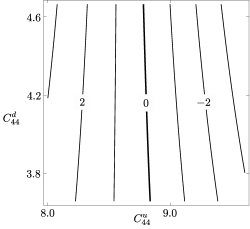
Figure 13: Dr2/1027subscriptD𝑟2superscript1027\mathrm{D}_{r2}/10^{27} , on the left, and Dr2/1020subscriptD𝑟2superscript1020\mathrm{D}_{r2}/10^{20} , on the right, defined in expression (17), as a function of the elasticity parameters, C44usuperscriptsubscript𝐶44𝑢C_{44}^{u} and C44dsuperscriptsubscript𝐶44𝑑C_{44}^{d} , where ω=60s1𝜔60superscripts1\omega=60~{}{\rm s}^{-1} and vr=1786m/ssubscript𝑣𝑟1786msv_{r}=1786~{}{\rm m}/{\rm s} , and where ω=15s1𝜔15superscripts1\omega=15~{}{\rm s}^{-1} and vr=1869m/ssubscript𝑣𝑟1869msv_{r}=1869~{}{\rm m}/{\rm s} , for left and right, respectively. The values on the horizontal and vertical axes are to be multiplied by 109superscript10910^{9} and 1010superscript101010^{10} , respectively. The near vertical contours in both plots indicate sensitivity to C44usuperscriptsubscript𝐶44𝑢C_{44}^{u} and little sensitivity to C44dsuperscriptsubscript𝐶44𝑑C_{44}^{d} .

3.2 Sensitivity of dispersion relation

We wish to examine effects of elasticity parameters and layer thickness on the dispersion relation, for various frequencies and different modes. To do so, we examine effects of these quantities on the value of Dr2subscriptD𝑟2\mathrm{D}_{r2} , defined in expression (17). Specifically, we examine Dr2subscriptD𝑟2\mathrm{D}_{r2} as a function of C44dsuperscriptsubscript𝐶44𝑑C_{44}^{d} and C44usuperscriptsubscript𝐶44𝑢C_{44}^{u} , for three distinct frequencies and for fixed values of vrsubscript𝑣𝑟v_{r} , which correspond to particular modes.
Refer to caption
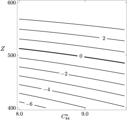
Figure 14: Dr2/1020subscriptD𝑟2superscript1020\mathrm{D}_{r2}/10^{20} , defined in expression (17), as a function of the elasticity parameter, C44usuperscriptsubscript𝐶44𝑢C_{44}^{u} , and layer thickness, Z𝑍Z , for ω=5s1𝜔5superscripts1\omega=5~{}{\rm s}^{-1} and vr=3069m/ssubscript𝑣𝑟3069msv_{r}=3069~{}{\rm m}/{\rm s} . The values on the horizontal axis are to be multiplied by 109superscript10910^{9} . The sloping zero contour indicate sensitivity to both C44usuperscriptsubscript𝐶44𝑢C_{44}^{u} and Z𝑍Z .

The contour maps of Figures 121315 and 16 illustrate the sensitivity of the dispersion relation by the slope of the zero contour line for quasi-Rayleigh waves. These plots, and their interpretation, are analogous to Figures 36.

Let us examine the numerical solutions for the quasi-Rayleigh wave dispersion relation for the high-frequency and low-frequency cases. We use these solutions to investigate the relative sensitivities of the quasi-Rayleigh wave to the elasticity parameter in the upper layer and in the lower halfspace, as well as to the elasticity parameter in the upper layer and to the layer thickness.

We begin by considering the layer and halfspace elasticity parameters. For the high-speed case, we consider the seventh root of the left plot of Figure 9, which is vr=3705m/ssubscript𝑣𝑟3705msv_{r}=3705~{}{\rm m}/{\rm s} , and the third root of the right plot of Figure 9, which is vr=3937m/ssubscript𝑣𝑟3937msv_{r}=3937~{}{\rm m}/{\rm s} . The left and right plots of Figure 12 are the corresponding contour plots of Dr2/1020subscriptD𝑟2superscript1020\mathrm{D}_{r2}/10^{20} with varying C44usuperscriptsubscript𝐶44𝑢C_{44}^{u} and C44dsuperscriptsubscript𝐶44𝑑C_{44}^{d} . In both cases, Dr2subscriptD𝑟2\mathrm{D}_{r2} is sensitive to C44usuperscriptsubscript𝐶44𝑢C_{44}^{u} and C44dsuperscriptsubscript𝐶44𝑑C_{44}^{d} . However, the right plot of Figure 12, which depicts a lower frequency and high speed, indicates a greater sensitivity to C44dsuperscriptsubscript𝐶44𝑑C_{44}^{d} .

Then, we consider Figure 11, which is the corresponding plot of Dr2/1019subscriptD𝑟2superscript1019\mathrm{D}_{r2}/10^{19} , whose frequency and speed is lower than the right plot of Figure 12. In this case, we observe that the determinant is also sensitive to both C44usuperscriptsubscript𝐶44𝑢C_{44}^{u} and C44dsuperscriptsubscript𝐶44𝑑C_{44}^{d} .

For the low-speed case, we observe different sensitivities. Let us examine the first root of the left plot of Figure 9, which is vr=1786m/ssubscript𝑣𝑟1786msv_{r}=1786~{}{\rm m}/{\rm s} , and the first root of the right plot of Figure 9, which is vr=1869m/ssubscript𝑣𝑟1869msv_{r}=1869~{}{\rm m}/{\rm s} . Following the corresponding plot of Figure 13, we see that there are near vertical zero lines. This indicates that there is a greater sensitivity C44usuperscriptsubscript𝐶44𝑢C_{44}^{u} but lower sensitivity to C44dsuperscriptsubscript𝐶44𝑑C_{44}^{d} for both frequencies.

Next, we consider the layer elasticity parameter and the layer thickness. Using the high-speed roots of expression (17), we observe sensitivity to both C44usuperscriptsubscript𝐶44𝑢C_{44}^{u} and Z𝑍Z , in the high-frequency and low-frequency cases, which are depicted in Figure 15. Using low-speed roots in Figure 16, we observe sensitivity in the right plot to both C44usuperscriptsubscript𝐶44𝑢C_{44}^{u} and Z𝑍Z. However, the left plot of Figure 16 has no sensitivity to Z𝑍Z since, regardless of Z𝑍Z , the fundamental-mode speed is asymptotic to the quasi-Rayleigh wave speed in the layer for higher frequencies.

We consider Figure 14 as well, which is the corresponding plot of Dr2/1020subscriptD𝑟2superscript1020\mathrm{D}_{r2}/10^{20} , whose frequency and speed is lower than the right plot of Figure 15. In this case, we observe that the determinant is sensitive to both C44usuperscriptsubscript𝐶44𝑢C_{44}^{u} and C44dsuperscriptsubscript𝐶44𝑑C_{44}^{d} .

Refer to caption
Refer to caption
Figure 15: Dr2/1021subscriptD𝑟2superscript1021\mathrm{D}_{r2}/10^{21} , defined in expression (17), as a function of the elasticity parameters, C44usuperscriptsubscript𝐶44𝑢C_{44}^{u} , and layer thickness, Z𝑍Z , for ω=60s1𝜔60superscripts1\omega=60~{}{\rm s}^{-1} and vr=3705m/ssubscript𝑣𝑟3705msv_{r}=3705~{}{\rm m}/{\rm s} , on the left, and for ω=15s1𝜔15superscripts1\omega=15~{}{\rm s}^{-1} and vr=3937m/ssubscript𝑣𝑟3937msv_{r}=3937~{}{\rm m}/{\rm s} , on the right. The values on the horizontal axis is to be multiplied by 109superscript10910^{9} . The sloping contours indicate sensitivity to both C44usuperscriptsubscript𝐶44𝑢C_{44}^{u} and Z𝑍Z .
Refer to caption
Refer to caption
Figure 16: Dr2/1028subscriptD𝑟2superscript1028\mathrm{D}_{r2}/10^{28} , on the left, and Dr2/1021subscriptD𝑟2superscript1021\mathrm{D}_{r2}/10^{21} , defined in expression (17), on the right, as a function of the elasticity parameter, C44usuperscriptsubscript𝐶44𝑢C_{44}^{u} , and layer thickness, Z𝑍Z , where ω=60s1𝜔60superscripts1\omega=60~{}{\rm s}^{-1} and vr=1786m/ssubscript𝑣𝑟1786msv_{r}=1786~{}{\rm m}/{\rm s} , and where ω=15s1𝜔15superscripts1\omega=15~{}{\rm s}^{-1} and vr=1869m/ssubscript𝑣𝑟1869msv_{r}=1869~{}{\rm m}/{\rm s} , for the left and right plots, respectively. The values on the horizontal axis is to be multiplied by 109superscript10910^{9} . The sloping zero contour in the lower frequency plot indicates sensitivity to both C44usuperscriptsubscript𝐶44𝑢C_{44}^{u} and Z𝑍Z while the vertical zero contour in the higher frequency plot indicates sensitivity to C44usuperscriptsubscript𝐶44𝑢C_{44}^{u} but no sensitivity to Z𝑍Z .

Additionally, Figure 15 is similar to Figure 5. The periodicity that shows up on the left plot of Figure 15 is due to the periodicity in Dr2subscript𝐷𝑟2D_{r2} . Furthermore, the left plot of Figure 16 is distinct from the left plot of Figure 6. The distinction is due to differences in asymptotic behaviour of the fundamental mode at high frequencies for the dispersion curves of Love and quasi-Rayleigh waves.

4 Conclusions

4.1 Background examination

In this paper, we study the sensitivity of Love waves and quasi-Rayleigh waves to model parameters based on their exact dispersion relations. Both are guided waves in an elastic layer constrained by a vacuum and an elastic halfspace. According to presented computations, and as illustrated in Figures 2 and 10, the dispersion relations for the Love and quasi-Rayleigh waves imply that their speeds vary with frequency and differ from one another. Thus, their arrival times should be distinct on a seismic record, which—together with the fact that their polarizations are orthogonal to one other—makes them independent sources of information to infer model parameters.

The speeds of both Love and quasi-Rayleigh waves, whose roots are depicted in Figures 1 and 9, respectively, are obtained from their dispersion relations. In the high-frequency case, the fundamental Love-wave mode has a speed that is slightly greater than the S𝑆S-wave speed in the layer. In the low-frequency case, its speed is slightly lower than the S𝑆S-wave speed in the halfspace. The highest-mode speeds of both the Love wave and the quasi-Rayleigh wave are less than the S𝑆S-wave speed in the halfspace.

The dispersion curves for Love waves and quasi-Rayleigh waves are given in Figure 2 and Figure 10, respectively. In the latter figure—and in agreement with Figure 10.14 of Udías [3]—the fundamental mode has all frequencies, which means that it has no cutoff frequency. For high frequency, the fundamental-mode speed asymptotically approaches the classical Rayleigh-wave speed in the layer, and—in the limit as ω0𝜔0\omega\rightarrow 0 —that speed approaches the classical Rayleigh-wave speed in the halfspace.

We review the dispersion relation for Love waves and provide the details in appendices of the derivation of the dispersion relation for quasi-Rayleigh waves, including details of the expansion of the 6×6666\times 6 matrix and its determinant. We compare our results to several past studies, including the one of Love [7], which assumes incompressibility, and the one of Udías [3], in which we found errors in the equations, though not in the dispersion-curve plots. Unlike Love [7], who assumes incompressibility, Udías [3], who assumes a Poisson’s ratio of 1/4141/4 , and Fu [6], who studies limiting cases, we do not make any simplifying assumptions prior to calculations for the study of sensitivity.

In the case of quasi-Rayleigh waves, and in the context of the 6×6666\times 6 determinant, we show that the solutions ru=0superscript𝑟𝑢0r^{u}=0 and su=0superscript𝑠𝑢0s^{u}=0 have zero displacements, and hence, can be considered trivial solutions.

4.2 Sensitivity results

Our results demonstrate the sensitivity of the Love wave and quasi-Rayleigh wave dispersion relations to elasticity parameters and layer thickness. We conclude that the fundamental mode is mainly sensitive to the upper layer properties while higher modes are sensitive to both the upper layer and lower halfspace properties. Within each mode the lower frequencies are more sensitive to the lower halfspace than are higher frequencies.

We do not consider sensitivity to C11subscript𝐶11C_{11} since we remain within the elasticity parameters common for both the Love and quasi-Rayleigh waves, nor do we examine the sensitivity to ρ𝜌\rho . Sensitivities to C11subscript𝐶11C_{11} and ρ𝜌\rho are obtainable by similar procedures. However, according to Lucena and Taioli [1], the dispersion curves are sensitive to neither of them.

In the case of Love waves, we formulate and examine the absolute value of a dimensionless sensitivity coefficient given in terms of partial derivatives of the Love-wave dispersion relation with respect to dimensionless variables, ν𝜈\nu and θ𝜃\theta . From these results, we perform an analysis to deduce the optimum frequency, ω0subscript𝜔0\omega_{0} , to obtain Z𝑍Z from a given mode.

Our results, in particular, Figures 278 and 10, allow us to infer data-acquisition information. This can be achieved by considering frequencies required to increase the number of modes. Using this information, we may calibrate sources and receivers to record different modes. For example, at ω=30s1𝜔30superscripts1\omega=30~{}{\rm s}^{-1} , we can see two Love-wave modes and four quasi-Rayleigh-wave modes.

5 Future work

Given dispersion relations of the Love and the quasi-Rayleigh waves, we expect to invert the measurements of speed for elasticity parameters and mass densities of both the layer and the halfspace, as well as for the layer thickness. Explicit expressions presented in this paper allow us to formulate the inverse problem and examine the sensitivity of its solution. In particular, the presence of two types of waves lends itself to the formulation of a joint inversion, which exploits the redundancy of information. The presented study of the Love and quasi-Rayleigh wave sensitivities allows us to gain an insight into their combination, which appears explicitly in such an inversion.

In further studies, we could formulate dispersion relations for the case of an anisotropic layer and an anisotropic halfspace. Such a formulation would require modified boundary conditions and equations of motion. Further insights into such issues are given by Babich and Kiselev [8].

Acknowledgments

We wish to acknowledge discussions with Adrian Bogacz, Tomasz Danek and Michael Rochester. We also acknowledge the graphical support of Elena Patarini. Also, we wish to acknowledge insightful suggestions of Paul Martin, as the editor, and the two anonymous reviewers. This research was performed in the context of The Geomechanics Project supported by Husky Energy. Also, this research was partially supported by the Natural Sciences and Engineering Research Council of Canada, grant 238416-2013.

References

  • [1] R. F. de Lucena and F. Taioli. Rayleigh wave modeling: A study of dispersion curve sensitivity and methodology for calculating an initial model to be included in an inversion algorithm. Journal of Applied Geophysics, 108:140–151, 2014.
  • [2] M. A. Slawinski. Waves and rays in seismology: Answers to unasked questions. World Scientific, 2016.
  • [3] A. Udías. Principles of seismology. Cambridge University Press, 1999.
  • [4] O. Novotný. Methods of computing the partial derivatives of dispersion curves. Pageoph, 114:765–774, 1976.
  • [5] A. Ben-Menahem and S. J. Singh. Seismic waves and sources. Dover, Mineola, N.Y., 2nd edition, 2000.
  • [6] C. Y. Fu. Studies on seismic waves: II. Rayleigh waves in a superficial layer. Geophysics, 11(1):10–23, 1946.
  • [7] A. E. H. Love. Some problems of geodynamics. Cambridge University Press, 1911.
  • [8] V. M. Babich and A. P. Kiselev. Elastic waves: High-frequency theory (in Russian). BHV St. Petersburg, 2014.
  • [9] A. W. Lee. The effect of geological structure upon microseismic disturbance. Geophysical Journal International, 3:85–105, 1932.

Appendix A Formulation of quasi-Rayleigh waves

Appendix A.1 Material properties and wave equations

555The formulation in this section is similar to that of Udías [3, Section 10.4] except that we set x3subscript𝑥3x_{3} to be positive downwards with the free surface at x3=0subscript𝑥30x_{3}=0 and interface at x3=Zsubscript𝑥3𝑍x_{3}=Z , whereas Udías [3] sets x3subscript𝑥3x_{3} to be positive upwards with the free surface at x3=Hsubscript𝑥3𝐻x_{3}=H and interface at x3=0subscript𝑥30x_{3}=0 . More importantly, unlike Udías [3], we do not restrict Poisson’s ratio in the layer and in the halfspace to 1/4141/4 . Also we found some errors in Udías’s equations.

Using the Helmholtz decomposition theorem, we express the displacements as

uμ=𝒫μ+×𝓢μ,u1μ=𝒫μx1𝒮μx3,u3μ=𝒫μx3+𝒮μx1,u2μ=0,μ=u,d,formulae-sequencesuperscript𝑢𝜇superscript𝒫𝜇superscript𝓢𝜇formulae-sequencesuperscriptsubscript𝑢1𝜇superscript𝒫𝜇subscript𝑥1superscript𝒮𝜇subscript𝑥3formulae-sequencesuperscriptsubscript𝑢3𝜇superscript𝒫𝜇subscript𝑥3superscript𝒮𝜇subscript𝑥1formulae-sequencesuperscriptsubscript𝑢2𝜇0𝜇𝑢𝑑u^{\mu}=\nabla{\mathcal{P}}^{\mu}+\nabla\times\mbox{\boldmath${\mathcal{S}}$}^{\mu}\,,\quad u_{1}^{\mu}=\frac{\partial{\mathcal{P}}^{\mu}}{\partial x_{1}}-\frac{\partial{\mathcal{S}}^{\mu}}{\partial x_{3}}\,,\quad u_{3}^{\mu}=\frac{\partial{\mathcal{P}}^{\mu}}{\partial x_{3}}+\frac{\partial{\mathcal{S}}^{\mu}}{\partial x_{1}}\,,\quad u_{2}^{\mu}=0\,,\,\,\mu=u,d, (18)

where we use the gauge condition outlined in Slawinski [2, Section 6.2] and set 𝒮2μ=𝒮μsuperscriptsubscript𝒮2𝜇superscript𝒮𝜇{\mathcal{S}}_{2}^{\mu}={\mathcal{S}}^{\mu} , for brevity. 𝒫μsuperscript𝒫𝜇\mathcal{P}^{\mu} denotes the scalar potential and 𝓢μ=[𝒮1μ,𝒮2μ,𝒮3μ]superscript𝓢𝜇superscriptsubscript𝒮1𝜇superscriptsubscript𝒮2𝜇superscriptsubscript𝒮3𝜇\mbox{\boldmath${\mathcal{S}}$}^{\mu}=[{\mathcal{S}}_{1}^{\mu},{\mathcal{S}}_{2}^{\mu},{\mathcal{S}}_{3}^{\mu}] denotes the vector potential, which herein is 𝓢μ=[0,𝒮μ,0]superscript𝓢𝜇0superscript𝒮𝜇0\mbox{\boldmath${\mathcal{S}}$}^{\mu}=[0,{\mathcal{S}}^{\mu},0] . Potentials allow us to consider the coupling between the P𝑃P and SV𝑆𝑉SV waves. The pertinent wave equations are

2𝒫μ1(αμ)22𝒫μt2=0,2𝒮μ1(βμ)22𝒮μt2=0,μ=u,d,formulae-sequencesuperscript2superscript𝒫𝜇1superscriptsuperscript𝛼𝜇2superscript2superscript𝒫𝜇superscript𝑡20formulae-sequencesuperscript2superscript𝒮𝜇1superscriptsuperscript𝛽𝜇2superscript2superscript𝒮𝜇superscript𝑡20𝜇𝑢𝑑\nabla^{2}{\mathcal{P}}^{\mu}-\frac{1}{(\alpha^{\mu})^{2}}\frac{\partial^{2}{\mathcal{P}}^{\mu}}{\partial t^{2}}=0\,\,,\,\,\,\nabla^{2}{\mathcal{S}}^{\mu}-\frac{1}{(\beta^{\mu})^{2}}\frac{\partial^{2}{\mathcal{S}}^{\mu}}{\partial t^{2}}=0\,,\,\,\,\mu=u,d, (19)

which correspond to the P𝑃P waves and SV𝑆𝑉SV waves, respectively.

Appendix A.2 Solutions of wave equations

Let the trial solutions for the corresponding wave equations be

𝒫μ=Aμ(x3)exp(ι(κx1ωt)),μ=u,d,formulae-sequencesuperscript𝒫𝜇superscript𝐴𝜇subscript𝑥3𝜄𝜅subscript𝑥1𝜔𝑡𝜇𝑢𝑑{\mathcal{P}}^{\mu}=A^{\mu}(x_{3})\exp(\iota(\kappa x_{1}-\omega t))\,,\quad\mu=u,d\,, (20)
𝒮μ=Bμ(x3)exp(ι(κx1ωt)),μ=u,d.formulae-sequencesuperscript𝒮𝜇superscript𝐵𝜇subscript𝑥3𝜄𝜅subscript𝑥1𝜔𝑡𝜇𝑢𝑑{\mathcal{S}}^{\mu}=B^{\mu}(x_{3})\exp(\iota(\kappa x_{1}-\omega t))\,,\quad\mu=u,d\,. (21)

Inserting solutions (20) and (21) into equations (19) leads to

d2Aμdx32+(ω2(αμ)2κ2)Aμ=0,d2Bμdx32+(ω2(βμ)2κ2)Bμ=0,μ=u,d,formulae-sequencesuperscriptd2superscript𝐴𝜇dsuperscriptsubscript𝑥32superscript𝜔2superscriptsuperscript𝛼𝜇2superscript𝜅2superscript𝐴𝜇0formulae-sequencesuperscriptd2superscript𝐵𝜇dsuperscriptsubscript𝑥32superscript𝜔2superscriptsuperscript𝛽𝜇2superscript𝜅2superscript𝐵𝜇0𝜇𝑢𝑑\frac{\,{\rm d}^{2}A^{\mu}}{\,{\rm d}x_{3}^{2}}+\left(\frac{\omega^{2}}{(\alpha^{\mu})^{2}}-\kappa^{2}\right)A^{\mu}=0\,,\,\,\,\frac{\,{\rm d}^{2}B^{\mu}}{\,{\rm d}x_{3}^{2}}+\left(\frac{\omega^{2}}{(\beta^{\mu})^{2}}-\kappa^{2}\right)B^{\mu}=0\,,\,\,\,\mu=u,d\,,

which are ordinary differential equations for amplitudes Aμsuperscript𝐴𝜇A^{\mu} and Bμsuperscript𝐵𝜇B^{\mu} . Similarly to the derivation of Love waves, we require displacements to decay within the halfspace. Expressions (18), which denote displacements, entail

κ2ω2/(αd)2>0andκ2ω2/(βd)2>0.formulae-sequencesuperscript𝜅2superscript𝜔2superscriptsuperscript𝛼𝑑20andsuperscript𝜅2superscript𝜔2superscriptsuperscript𝛽𝑑20\kappa^{2}-\omega^{2}/(\alpha^{d})^{2}>0\quad{\rm and}\quad\kappa^{2}-\omega^{2}/(\beta^{d})^{2}>0\,.

Thus, we obtain four general solutions, which we write as

Au=C1exp(ιω2(αu)2κ2x3)+C2exp(ιω2(αu)2κ2x3),superscript𝐴𝑢subscript𝐶1𝜄superscript𝜔2superscriptsuperscript𝛼𝑢2superscript𝜅2subscript𝑥3subscript𝐶2𝜄superscript𝜔2superscriptsuperscript𝛼𝑢2superscript𝜅2subscript𝑥3A^{u}=C_{1}\exp\left(-\iota\sqrt{\frac{\omega^{2}}{(\alpha^{u})^{2}}-\kappa^{2}}\,x_{3}\right)+C_{2}\exp\left(\iota\sqrt{\frac{\omega^{2}}{(\alpha^{u})^{2}}-\kappa^{2}}\,x_{3}\right)\,, (22)
Adsuperscript𝐴𝑑\displaystyle A^{d} =C4exp(κ2ω2(αd)2x3),absentsubscript𝐶4superscript𝜅2superscript𝜔2superscriptsuperscript𝛼𝑑2subscript𝑥3\displaystyle=C_{4}\exp\left(-\sqrt{\kappa^{2}-\frac{\omega^{2}}{(\alpha^{d})^{2}}}\,x_{3}\right)\,,
Busuperscript𝐵𝑢\displaystyle B^{u} =D1exp(ιω2(βu)2κ2x3)+D2exp(ιω2(βu)2κ2x3),absentsubscript𝐷1𝜄superscript𝜔2superscriptsuperscript𝛽𝑢2superscript𝜅2subscript𝑥3subscript𝐷2𝜄superscript𝜔2superscriptsuperscript𝛽𝑢2superscript𝜅2subscript𝑥3\displaystyle=D_{1}\exp\left(-\iota\sqrt{\frac{\omega^{2}}{(\beta^{u})^{2}}-\kappa^{2}}\,x_{3}\right)+D_{2}\exp\left(\iota\sqrt{\frac{\omega^{2}}{(\beta^{u})^{2}}-\kappa^{2}}\,x_{3}\right)\,,
Bdsuperscript𝐵𝑑\displaystyle B^{d} =D4exp(κ2ω2(βd)2x3).absentsubscript𝐷4superscript𝜅2superscript𝜔2superscriptsuperscript𝛽𝑑2subscript𝑥3\displaystyle=D_{4}\exp\left(-\sqrt{\kappa^{2}-\frac{\omega^{2}}{(\beta^{d})^{2}}}\,x_{3}\right)\,.

Our assumption about the behaviour of solutions in the halfspace forces rdsuperscript𝑟𝑑r^{d} and sdsuperscript𝑠𝑑s^{d} to be real. Thus, we write the nonzero components of the displacement vector as

u1d=superscriptsubscript𝑢1𝑑absent\displaystyle u_{1}^{d}= 𝒫dx1𝒮dx3superscript𝒫𝑑subscript𝑥1superscript𝒮𝑑subscript𝑥3\displaystyle\frac{\partial{\mathcal{P}}^{d}}{\partial x_{1}}-\frac{\partial{\mathcal{S}}^{d}}{\partial x_{3}} (23)
=\displaystyle= [ικC4exp(κrdx3)+D4κsdexp(κsdx3)]exp(ι(κx1ωt)),delimited-[]𝜄𝜅subscript𝐶4𝜅superscript𝑟𝑑subscript𝑥3subscript𝐷4𝜅superscript𝑠𝑑𝜅superscript𝑠𝑑subscript𝑥3𝜄𝜅subscript𝑥1𝜔𝑡\displaystyle\left[\iota\kappa C_{4}\exp\left(-\kappa r^{d}x_{3}\right)+D_{4}\kappa s^{d}\exp\left(-\kappa s^{d}x_{3}\right)\right]\exp(\iota(\kappa x_{1}-\omega t))\,,
u3d=superscriptsubscript𝑢3𝑑absent\displaystyle u_{3}^{d}= 𝒫dx3+𝒮dx1superscript𝒫𝑑subscript𝑥3superscript𝒮𝑑subscript𝑥1\displaystyle\frac{\partial{\mathcal{P}}^{d}}{\partial x_{3}}+\frac{\partial{\mathcal{S}}^{d}}{\partial x_{1}} (24)
=\displaystyle= [C4κrdexp(κrdx3)+ικD4exp(κsdx3)]exp(ι(κx1ωt)),delimited-[]subscript𝐶4𝜅superscript𝑟𝑑𝜅superscript𝑟𝑑subscript𝑥3𝜄𝜅subscript𝐷4𝜅superscript𝑠𝑑subscript𝑥3𝜄𝜅subscript𝑥1𝜔𝑡\displaystyle\left[-C_{4}\kappa r^{d}\exp\left(-\kappa r^{d}x_{3}\right)+\iota\kappa D_{4}\exp\left(-\kappa s^{d}x_{3}\right)\right]\exp(\iota(\kappa x_{1}-\omega t))\,,
u1u=superscriptsubscript𝑢1𝑢absent\displaystyle u_{1}^{u}= 𝒫ux1𝒮ux3superscript𝒫𝑢subscript𝑥1superscript𝒮𝑢subscript𝑥3\displaystyle\frac{\partial{\mathcal{P}}^{u}}{\partial x_{1}}-\frac{\partial{\mathcal{S}}^{u}}{\partial x_{3}} (25)
=\displaystyle= [ικC1exp(ικrux3)+ικC2exp(ικrux3)\displaystyle\left[\iota\kappa C_{1}\exp(-\iota\kappa r^{u}x_{3})+\iota\kappa C_{2}\exp(\iota\kappa r^{u}x_{3})\right.
+ικsuD1exp(ικsux3)ικsuD2exp(ικsux3)]exp(ι(κx1ωt)),\displaystyle\left.\qquad+\,\iota\kappa s^{u}D_{1}\exp(-\iota\kappa s^{u}x_{3})-\iota\kappa s^{u}D_{2}\exp(\iota\kappa s^{u}x_{3})\right]\exp(\iota(\kappa x_{1}-\omega t))\,,
u3u=superscriptsubscript𝑢3𝑢absent\displaystyle u_{3}^{u}= 𝒫ux3+𝒮ux1superscript𝒫𝑢subscript𝑥3superscript𝒮𝑢subscript𝑥1\displaystyle\frac{\partial{\mathcal{P}}^{u}}{\partial x_{3}}+\frac{\partial{\mathcal{S}}^{u}}{\partial x_{1}} (26)
=\displaystyle= [ικruC1exp(ικrux3)+ικruC2exp(ικrux3)\displaystyle\left[-\iota\kappa r^{u}C_{1}\exp(-\iota\kappa r^{u}x_{3})+\iota\kappa r^{u}C_{2}\exp(\iota\kappa r^{u}x_{3})\right.
+ικD1exp(ικsux3)+ικD2exp(ικsux3)]exp(ι(κx1ωt)),\displaystyle\left.\qquad+\,\iota\kappa D_{1}\exp(-\iota\kappa s^{u}x_{3})+\iota\kappa D_{2}\exp(\iota\kappa s^{u}x_{3})\right]\exp(\iota(\kappa x_{1}-\omega t))\,,

which allows us to apply the boundary conditions.

Appendix A.3 Boundary conditions

Let us examine expressions (23)–(26) in view of Hooke’s law,

σij=λδijk=13εkk+2μεij=(C112C44)δijk=13ukxk+C44(uixj+ujxi),subscript𝜎𝑖𝑗𝜆subscript𝛿𝑖𝑗superscriptsubscript𝑘13subscript𝜀𝑘𝑘2𝜇subscript𝜀𝑖𝑗subscript𝐶112subscript𝐶44subscript𝛿𝑖𝑗superscriptsubscript𝑘13subscript𝑢𝑘subscript𝑥𝑘subscript𝐶44subscript𝑢𝑖subscript𝑥𝑗subscript𝑢𝑗subscript𝑥𝑖\sigma_{ij}=\lambda\delta_{ij}\sum_{k=1}^{3}\varepsilon_{kk}+2\mu\varepsilon_{ij}=(C_{11}-2C_{44})\,\delta_{ij}\sum_{k=1}^{3}\frac{\partial u_{k}}{\partial x_{k}}+C_{44}\left(\frac{\partial u_{i}}{\partial x_{j}}+\frac{\partial u_{j}}{\partial x_{i}}\right)\,, (27)

and the boundary conditions at x3=0subscript𝑥30x_{3}=0 , which are σ33u=σ31u=0superscriptsubscript𝜎33𝑢superscriptsubscript𝜎31𝑢0\sigma_{33}^{u}=\sigma_{31}^{u}=0 ; hence, the first condition implies

σ31u|x3=0=0u1ux3|x3=0=u3ux1|x3=0.evaluated-atsuperscriptsubscript𝜎31𝑢subscript𝑥300evaluated-atsuperscriptsubscript𝑢1𝑢subscript𝑥3subscript𝑥30evaluated-atsuperscriptsubscript𝑢3𝑢subscript𝑥1subscript𝑥30\left.\sigma_{31}^{u}\right|_{x_{3}=0}=0\Rightarrow\left.\frac{\partial u_{1}^{u}}{\partial x_{3}}\right|_{x_{3}=0}=-\left.\frac{\partial u_{3}^{u}}{\partial x_{1}}\right|_{x_{3}=0}\,.

Factoring out exp(ι(κx1ωt))𝜄𝜅subscript𝑥1𝜔𝑡\exp(\iota(\kappa x_{1}-\omega t)) , we write

κ2ruC1κ2ruC2+κ2(su)2D1+κ2(su)2D2=κ2ruC1+κ2ruC2+κ2D1+κ2D2,superscript𝜅2superscript𝑟𝑢subscript𝐶1superscript𝜅2superscript𝑟𝑢subscript𝐶2superscript𝜅2superscriptsuperscript𝑠𝑢2subscript𝐷1superscript𝜅2superscriptsuperscript𝑠𝑢2subscript𝐷2superscript𝜅2superscript𝑟𝑢subscript𝐶1superscript𝜅2superscript𝑟𝑢subscript𝐶2superscript𝜅2subscript𝐷1superscript𝜅2subscript𝐷2\kappa^{2}r^{u}C_{1}-\kappa^{2}r^{u}C_{2}+\kappa^{2}(s^{u})^{2}D_{1}+\kappa^{2}(s^{u})^{2}D_{2}=-\kappa^{2}r^{u}C_{1}+\kappa^{2}r^{u}C_{2}+\kappa^{2}D_{1}+\kappa^{2}D_{2}\,,

which, upon rearranging and factoring out κ2superscript𝜅2\kappa^{2} , we rewrite as

2ru(C1C2)+[(su)21](D1+D2)=0.2superscript𝑟𝑢subscript𝐶1subscript𝐶2delimited-[]superscriptsuperscript𝑠𝑢21subscript𝐷1subscript𝐷202r^{u}(C_{1}-C_{2})+[(s^{u})^{2}-1](D_{1}+D_{2})=0\,. (28)

The second condition implies

σ33u|x3=0=0[(C11u2C44u)(u1ux1+u3ux3)+2C44u(u3ux3)]|x3=0=0,evaluated-atsuperscriptsubscript𝜎33𝑢subscript𝑥300evaluated-atdelimited-[]superscriptsubscript𝐶11𝑢2superscriptsubscript𝐶44𝑢superscriptsubscript𝑢1𝑢subscript𝑥1superscriptsubscript𝑢3𝑢subscript𝑥32superscriptsubscript𝐶44𝑢superscriptsubscript𝑢3𝑢subscript𝑥3subscript𝑥300\left.\sigma_{33}^{u}\right|_{x_{3}=0}=0\Rightarrow\left.\left[(C_{11}^{u}-2C_{44}^{u})\left(\frac{\partial u_{1}^{u}}{\partial x_{1}}+\frac{\partial u_{3}^{u}}{\partial x_{3}}\right)+2C_{44}^{u}\left(\frac{\partial u_{3}^{u}}{\partial x_{3}}\right)\right]\right|_{x_{3}=0}=0\,,

which can be rearranged to

[(C11u2C44u)(u1ux1)+C11u(u3ux3)]|x3=0=0,evaluated-atdelimited-[]superscriptsubscript𝐶11𝑢2superscriptsubscript𝐶44𝑢superscriptsubscript𝑢1𝑢subscript𝑥1superscriptsubscript𝐶11𝑢superscriptsubscript𝑢3𝑢subscript𝑥3subscript𝑥300\left.\left[(C_{11}^{u}-2C_{44}^{u})\left(\frac{\partial u_{1}^{u}}{\partial x_{1}}\right)+C_{11}^{u}\left(\frac{\partial u_{3}^{u}}{\partial x_{3}}\right)\right]\right|_{x_{3}=0}=0\,,

and, upon factoring out κ2exp(ι(κx1ωt))superscript𝜅2𝜄𝜅subscript𝑥1𝜔𝑡\kappa^{2}\exp(\iota(\kappa x_{1}-\omega t)) , further reduces to

(C11u2C44u)[(C1+C2)su(D1D2)]+C11u[(ru)2(C1+C2)+su(D1D2)]=0.superscriptsubscript𝐶11𝑢2superscriptsubscript𝐶44𝑢delimited-[]subscript𝐶1subscript𝐶2superscript𝑠𝑢subscript𝐷1subscript𝐷2superscriptsubscript𝐶11𝑢delimited-[]superscriptsuperscript𝑟𝑢2subscript𝐶1subscript𝐶2superscript𝑠𝑢subscript𝐷1subscript𝐷20(C_{11}^{u}-2C_{44}^{u})\left[-(C_{1}+C_{2})-s^{u}(D_{1}-D_{2})\right]+C_{11}^{u}\left[-(r^{u})^{2}(C_{1}+C_{2})+s^{u}(D_{1}-D_{2})\right]=0\,. (29)

At x3=Zsubscript𝑥3𝑍x_{3}=Z , the boundary conditions are

u1u|x3=Zevaluated-atsuperscriptsubscript𝑢1𝑢subscript𝑥3𝑍\displaystyle u_{1}^{u}|_{x_{3}=Z} =u1d|x3=Z,u3u|x3=Z=u3d|x3=Z,formulae-sequenceabsentevaluated-atsuperscriptsubscript𝑢1𝑑subscript𝑥3𝑍evaluated-atsuperscriptsubscript𝑢3𝑢subscript𝑥3𝑍evaluated-atsuperscriptsubscript𝑢3𝑑subscript𝑥3𝑍\displaystyle=u_{1}^{d}|_{x_{3}=Z}\,,\quad u_{3}^{u}|_{x_{3}=Z}=u_{3}^{d}|_{x_{3}=Z}\,,
σ33u|x3=Zevaluated-atsuperscriptsubscript𝜎33𝑢subscript𝑥3𝑍\displaystyle\sigma_{33}^{u}|_{x_{3}=Z} =σ33d|x3=Z,σ31u|x3=Z=σ31d|x3=Z.formulae-sequenceabsentevaluated-atsuperscriptsubscript𝜎33𝑑subscript𝑥3𝑍evaluated-atsuperscriptsubscript𝜎31𝑢subscript𝑥3𝑍evaluated-atsuperscriptsubscript𝜎31𝑑subscript𝑥3𝑍\displaystyle=\sigma_{33}^{d}|_{x_{3}=Z}\,,\quad\sigma_{31}^{u}|_{x_{3}=Z}=\sigma_{31}^{d}|_{x_{3}=Z}\,.

Factoring out  κexp(ι(κx1ωt))𝜅𝜄𝜅subscript𝑥1𝜔𝑡\kappa\exp(\iota(\kappa x_{1}-\omega t)) , the first condition becomes

ιC1exp(ικruZ)+ιC2exp(ικruZ)+ιsuD1𝜄subscript𝐶1𝜄𝜅superscript𝑟𝑢𝑍𝜄subscript𝐶2𝜄𝜅superscript𝑟𝑢𝑍𝜄superscript𝑠𝑢subscript𝐷1\displaystyle\iota C_{1}\exp(-\iota\kappa r^{u}Z)+\iota C_{2}\exp(\iota\kappa r^{u}Z)+\iota s^{u}D_{1} exp(ικsuZ)ιsuD2exp(ικsuZ)𝜄𝜅superscript𝑠𝑢𝑍𝜄superscript𝑠𝑢subscript𝐷2𝜄𝜅superscript𝑠𝑢𝑍\displaystyle\exp(-\iota\kappa s^{u}Z)-\iota s^{u}D_{2}\exp(\iota\kappa s^{u}Z)
=\displaystyle= ιC4exp(κrdZ)+sdD4exp(κsdZ).𝜄subscript𝐶4𝜅superscript𝑟𝑑𝑍superscript𝑠𝑑subscript𝐷4𝜅superscript𝑠𝑑𝑍\displaystyle\,\iota C_{4}\exp(-\kappa r^{d}Z)+s^{d}D_{4}\exp(-\kappa s^{d}Z)\,. (30)

Similarly, the second condition implies

ιruC1exp(ικruZ)+ιruC2exp(ικruZ)+ι𝜄superscript𝑟𝑢subscript𝐶1𝜄𝜅superscript𝑟𝑢𝑍𝜄superscript𝑟𝑢subscript𝐶2𝜄𝜅superscript𝑟𝑢𝑍𝜄\displaystyle-\iota r^{u}C_{1}\exp(-\iota\kappa r^{u}Z)+\iota r^{u}C_{2}\exp(\iota\kappa r^{u}Z)+\iota D1exp(ικsuZ)+ιD2exp(ικsuZ)subscript𝐷1𝜄𝜅superscript𝑠𝑢𝑍𝜄subscript𝐷2𝜄𝜅superscript𝑠𝑢𝑍\displaystyle D_{1}\exp(-\iota\kappa s^{u}Z)+\iota D_{2}\exp(\iota\kappa s^{u}Z)
=\displaystyle= rdC4exp(κrdZ)+ιD4exp(κsdZ).superscript𝑟𝑑subscript𝐶4𝜅superscript𝑟𝑑𝑍𝜄subscript𝐷4𝜅superscript𝑠𝑑𝑍\displaystyle-r^{d}C_{4}\exp(-\kappa r^{d}Z)+\iota D_{4}\exp(-\kappa s^{d}Z)\,. (31)

The third condition,

[(C11u2C44u)(u1ux1)+C11u(u3ux3)]|x3=Z=[(C11d2C44d)(u1dx1)+C11d(u3dx3)]|x3=Z,evaluated-atdelimited-[]superscriptsubscript𝐶11𝑢2superscriptsubscript𝐶44𝑢superscriptsubscript𝑢1𝑢subscript𝑥1superscriptsubscript𝐶11𝑢superscriptsubscript𝑢3𝑢subscript𝑥3subscript𝑥3𝑍evaluated-atdelimited-[]superscriptsubscript𝐶11𝑑2superscriptsubscript𝐶44𝑑superscriptsubscript𝑢1𝑑subscript𝑥1superscriptsubscript𝐶11𝑑superscriptsubscript𝑢3𝑑subscript𝑥3subscript𝑥3𝑍\left.\left[(C_{11}^{u}-2C_{44}^{u})\left(\frac{\partial u_{1}^{u}}{\partial x_{1}}\right)+C_{11}^{u}\left(\frac{\partial u_{3}^{u}}{\partial x_{3}}\right)\right]\right|_{x_{3}=Z}=\left.\left[(C_{11}^{d}-2C_{44}^{d})\left(\frac{\partial u_{1}^{d}}{\partial x_{1}}\right)+C_{11}^{d}\left(\frac{\partial u_{3}^{d}}{\partial x_{3}}\right)\right]\right|_{x_{3}=Z}\,,

upon factoring out κ2exp(ι(κx1ωt))superscript𝜅2𝜄𝜅subscript𝑥1𝜔𝑡\kappa^{2}\exp(\iota(\kappa x_{1}-\omega t)) , becomes

(C11u\displaystyle(C_{11}^{u} 2C44u)[C1exp(ικruZ)C2exp(ικruZ)suD1exp(ικsuZ)+suD2exp(ικsuZ)]\displaystyle-2C_{44}^{u})\left[-C_{1}\exp(-\iota\kappa r^{u}Z)-C_{2}\exp(\iota\kappa r^{u}Z)-s^{u}D_{1}\exp(-\iota\kappa s^{u}Z)+s^{u}D_{2}\exp(\iota\kappa s^{u}Z)\right]
+\displaystyle+\, C11u[(ru)2C1exp(ικruZ)(ru)2C2exp(ικruZ)+suD1exp(ικsuZ)suD2exp(ικsuZ)]superscriptsubscript𝐶11𝑢delimited-[]superscriptsuperscript𝑟𝑢2subscript𝐶1𝜄𝜅superscript𝑟𝑢𝑍superscriptsuperscript𝑟𝑢2subscript𝐶2𝜄𝜅superscript𝑟𝑢𝑍superscript𝑠𝑢subscript𝐷1𝜄𝜅superscript𝑠𝑢𝑍superscript𝑠𝑢subscript𝐷2𝜄𝜅superscript𝑠𝑢𝑍\displaystyle C_{11}^{u}\left[-(r^{u})^{2}C_{1}\exp(-\iota\kappa r^{u}Z)-(r^{u})^{2}C_{2}\exp(\iota\kappa r^{u}Z)+s^{u}D_{1}\exp(-\iota\kappa s^{u}Z)-s^{u}D_{2}\exp(\iota\kappa s^{u}Z)\right]
=(C11d2C44d)[C4exp(κrdZ)+ιsdD4exp(κsdZ)]absentsuperscriptsubscript𝐶11𝑑2superscriptsubscript𝐶44𝑑delimited-[]subscript𝐶4𝜅superscript𝑟𝑑𝑍𝜄superscript𝑠𝑑subscript𝐷4𝜅superscript𝑠𝑑𝑍\displaystyle=(C_{11}^{d}-2C_{44}^{d})\left[-C_{4}\exp(-\kappa r^{d}Z)+\iota s^{d}D_{4}\exp(-\kappa s^{d}Z)\right]
+C11d[(rd)2C4exp(κrdZ)ιsdD4exp(κsdZ)].superscriptsubscript𝐶11𝑑delimited-[]superscriptsuperscript𝑟𝑑2subscript𝐶4𝜅superscript𝑟𝑑𝑍𝜄superscript𝑠𝑑subscript𝐷4𝜅superscript𝑠𝑑𝑍\displaystyle\qquad+C_{11}^{d}\left[(r^{d})^{2}C_{4}\exp(-\kappa r^{d}Z)-\iota s^{d}D_{4}\exp(-\kappa s^{d}Z)\right]\,.

The fourth condition,

C44u(u1ux3+u3ux1)|x3=Z=C44d(u1dx3+u3dx1)|x3=Z,evaluated-atsuperscriptsubscript𝐶44𝑢superscriptsubscript𝑢1𝑢subscript𝑥3superscriptsubscript𝑢3𝑢subscript𝑥1subscript𝑥3𝑍evaluated-atsuperscriptsubscript𝐶44𝑑superscriptsubscript𝑢1𝑑subscript𝑥3superscriptsubscript𝑢3𝑑subscript𝑥1subscript𝑥3𝑍\left.C_{44}^{u}\left(\frac{\partial u_{1}^{u}}{\partial x_{3}}+\frac{\partial u_{3}^{u}}{\partial x_{1}}\right)\right|_{x_{3}=Z}=\left.C_{44}^{d}\left(\frac{\partial u_{1}^{d}}{\partial x_{3}}+\frac{\partial u_{3}^{d}}{\partial x_{1}}\right)\right|_{x_{3}=Z}\,,

implies

C44usuperscriptsubscript𝐶44𝑢\displaystyle C_{44}^{u} [ruC1exp(ικruZ)ruC2exp(ικruZ)+(su)2D1exp(ικsuZ)+(su)2D2exp(ικsuZ)\displaystyle\left[r^{u}C_{1}\exp(-\iota\kappa r^{u}Z)-r^{u}C_{2}\exp(\iota\kappa r^{u}Z)+(s^{u})^{2}D_{1}\exp(-\iota\kappa s^{u}Z)+(s^{u})^{2}D_{2}\exp(\iota\kappa s^{u}Z)\right.
+ruC1exp(ικruZ)ruC2exp(ικruZ)D1exp(ικsuZ)D2exp(ικsuZ)]\displaystyle\left.+\,r^{u}C_{1}\exp(-\iota\kappa r^{u}Z)-r^{u}C_{2}\exp(\iota\kappa r^{u}Z)-D_{1}\exp(-\iota\kappa s^{u}Z)-D_{2}\exp(\iota\kappa s^{u}Z)\right]
=C44d[ιrdC4exp(κrdZ)(sd)2D4exp(κsdZ)ιrdC4exp(κrdZ)D4exp(κsdZ)].absentsuperscriptsubscript𝐶44𝑑delimited-[]𝜄superscript𝑟𝑑subscript𝐶4𝜅superscript𝑟𝑑𝑍superscriptsuperscript𝑠𝑑2subscript𝐷4𝜅superscript𝑠𝑑𝑍𝜄superscript𝑟𝑑subscript𝐶4𝜅superscript𝑟𝑑𝑍subscript𝐷4𝜅superscript𝑠𝑑𝑍\displaystyle=C_{44}^{d}\left[-\iota r^{d}C_{4}\exp(-\kappa r^{d}Z)-(s^{d})^{2}D_{4}\exp(-\kappa s^{d}Z)-\iota r^{d}C_{4}\exp(-\kappa r^{d}Z)-D_{4}\exp(-\kappa s^{d}Z)\right]\,. (32)

For a notational convenience, we let

a:=κruZ,a=κrdZ,C1:=C1eιa,C2:=C2eιa,C4:=C4ea,formulae-sequenceassignsuperscript𝑎𝜅superscript𝑟𝑢𝑍formulae-sequence𝑎𝜅superscript𝑟𝑑𝑍formulae-sequenceassignsuperscriptsubscript𝐶1subscript𝐶1superscripte𝜄superscript𝑎formulae-sequenceassignsuperscriptsubscript𝐶2subscript𝐶2superscripte𝜄superscript𝑎assignsuperscriptsubscript𝐶4subscript𝐶4superscripte𝑎a^{\prime}:=\kappa r^{u}Z\,,a=\kappa r^{d}Z\,,C_{1}^{\prime}:=C_{1}\,{\rm e}^{-\iota a^{\prime}}\,,C_{2}^{\prime}:=C_{2}\,{\rm e}^{\iota a^{\prime}}\,,C_{4}^{\prime}:=C_{4}\,{\rm e}^{-a}\,, (33)
b:=κsuZ,b=κsdZ,D1:=D1eιb,D2:=D2eιb,D4:=D4eb.formulae-sequenceassignsuperscript𝑏𝜅superscript𝑠𝑢𝑍formulae-sequence𝑏𝜅superscript𝑠𝑑𝑍formulae-sequenceassignsuperscriptsubscript𝐷1subscript𝐷1superscripte𝜄superscript𝑏formulae-sequenceassignsuperscriptsubscript𝐷2subscript𝐷2superscripte𝜄superscript𝑏assignsuperscriptsubscript𝐷4subscript𝐷4superscripte𝑏b^{\prime}:=\kappa s^{u}Z\,,b=\kappa s^{d}Z\,,D_{1}^{\prime}:=D_{1}\,{\rm e}^{-\iota b^{\prime}}\,,D_{2}^{\prime}:=D_{2}\,{\rm e}^{\iota b^{\prime}}\,,D_{4}^{\prime}:=D_{4}\,{\rm e}^{-b}\,. (34)

Thus, conditions (28) to (32) can be written as

2rueιaC12rueιaC2+[(su)21]eιbD1+[(su)21]eιbD2=0,2superscript𝑟𝑢superscripte𝜄superscript𝑎superscriptsubscript𝐶12superscript𝑟𝑢superscripte𝜄superscript𝑎superscriptsubscript𝐶2delimited-[]superscriptsuperscript𝑠𝑢21superscripte𝜄superscript𝑏superscriptsubscript𝐷1delimited-[]superscriptsuperscript𝑠𝑢21superscripte𝜄superscript𝑏superscriptsubscript𝐷202r^{u}\,{\rm e}^{\iota a^{\prime}}C_{1}^{\prime}-2r^{u}\,{\rm e}^{-\iota a^{\prime}}C_{2}^{\prime}+[(s^{u})^{2}-1]\,{\rm e}^{\iota b^{\prime}}D_{1}^{\prime}+[(s^{u})^{2}-1]\,{\rm e}^{-\iota b^{\prime}}D_{2}^{\prime}=0\,, (35)
[(C11u\displaystyle[-(C_{11}^{u}- 2C44u)C11u(ru)2]eιaC1+[(C11u2C44u)C11u(ru)2]eιaC2\displaystyle 2C_{44}^{u})-C_{11}^{u}(r^{u})^{2}]\,{\rm e}^{\iota a^{\prime}}C_{1}^{\prime}+[-(C_{11}^{u}-2C_{44}^{u})-C_{11}^{u}(r^{u})^{2}]\,{\rm e}^{-\iota a^{\prime}}C_{2}^{\prime}
+2C44usueιbD12C44usueιbD2=0,2superscriptsubscript𝐶44𝑢superscript𝑠𝑢superscripte𝜄superscript𝑏superscriptsubscript𝐷12superscriptsubscript𝐶44𝑢superscript𝑠𝑢superscripte𝜄superscript𝑏superscriptsubscript𝐷20\displaystyle+2C_{44}^{u}s^{u}\,{\rm e}^{\iota b^{\prime}}D_{1}^{\prime}-2C_{44}^{u}s^{u}\,{\rm e}^{-\iota b^{\prime}}D_{2}^{\prime}=0\,, (36)
ιC1+ιC2+ιsuD1ιsuD2ιC4sdD4=0,𝜄superscriptsubscript𝐶1𝜄superscriptsubscript𝐶2𝜄superscript𝑠𝑢superscriptsubscript𝐷1𝜄superscript𝑠𝑢superscriptsubscript𝐷2𝜄superscriptsubscript𝐶4superscript𝑠𝑑superscriptsubscript𝐷40\iota C_{1}^{\prime}+\iota C_{2}^{\prime}+\iota s^{u}D_{1}^{\prime}-\iota s^{u}D_{2}^{\prime}-\iota C_{4}^{\prime}-s^{d}D_{4}^{\prime}=0\,, (37)
ιruC1+ιruC2+ιD1+ιD2+rdC4ιD4=0,𝜄superscript𝑟𝑢superscriptsubscript𝐶1𝜄superscript𝑟𝑢superscriptsubscript𝐶2𝜄superscriptsubscript𝐷1𝜄superscriptsubscript𝐷2superscript𝑟𝑑superscriptsubscript𝐶4𝜄superscriptsubscript𝐷40-\iota r^{u}C_{1}^{\prime}+\iota r^{u}C_{2}^{\prime}+\iota D_{1}^{\prime}+\iota D_{2}^{\prime}+r^{d}C_{4}^{\prime}-\iota D_{4}^{\prime}=0\,, (38)
(C11u\displaystyle-(C_{11}^{u} 2C44u)C1(C11u2C44u)C2(C11u2C44u)suD1+(C11u2C44u)suD2\displaystyle-2C_{44}^{u})C_{1}^{\prime}-(C_{11}^{u}-2C_{44}^{u})C_{2}^{\prime}-(C_{11}^{u}-2C_{44}^{u})s^{u}D_{1}^{\prime}+(C_{11}^{u}-2C_{44}^{u})s^{u}D_{2}^{\prime}
C11u(ru)2C1C11u(ru)2C2+C11usuD1C11usuD2+(C11d2C44d)C4superscriptsubscript𝐶11𝑢superscriptsuperscript𝑟𝑢2superscriptsubscript𝐶1superscriptsubscript𝐶11𝑢superscriptsuperscript𝑟𝑢2superscriptsubscript𝐶2superscriptsubscript𝐶11𝑢superscript𝑠𝑢superscriptsubscript𝐷1superscriptsubscript𝐶11𝑢superscript𝑠𝑢superscriptsubscript𝐷2superscriptsubscript𝐶11𝑑2superscriptsubscript𝐶44𝑑superscriptsubscript𝐶4\displaystyle-C_{11}^{u}(r^{u})^{2}C_{1}^{\prime}-C_{11}^{u}(r^{u})^{2}C_{2}^{\prime}+C_{11}^{u}s^{u}D_{1}^{\prime}-C_{11}^{u}s^{u}D_{2}^{\prime}+(C_{11}^{d}-2C_{44}^{d})C_{4}^{\prime}
ι(C11d2C44d)sdD4C11d(rd)2C4+ιC11dsdD4=0,𝜄superscriptsubscript𝐶11𝑑2superscriptsubscript𝐶44𝑑superscript𝑠𝑑superscriptsubscript𝐷4superscriptsubscript𝐶11𝑑superscriptsuperscript𝑟𝑑2superscriptsubscript𝐶4𝜄superscriptsubscript𝐶11𝑑superscript𝑠𝑑superscriptsubscript𝐷40\displaystyle\qquad-\iota(C_{11}^{d}-2C_{44}^{d})s^{d}D_{4}^{\prime}-C_{11}^{d}(r^{d})^{2}C_{4}^{\prime}+\iota C_{11}^{d}s^{d}D_{4}^{\prime}=0\,, (39)
C44usuperscriptsubscript𝐶44𝑢\displaystyle C_{44}^{u} ruC1C44uruC2+C44u(su)2D1+C44u(su)2D2+C44uruC1C44uruC2C44uD1C44uD2superscript𝑟𝑢superscriptsubscript𝐶1superscriptsubscript𝐶44𝑢superscript𝑟𝑢superscriptsubscript𝐶2superscriptsubscript𝐶44𝑢superscriptsuperscript𝑠𝑢2superscriptsubscript𝐷1superscriptsubscript𝐶44𝑢superscriptsuperscript𝑠𝑢2superscriptsubscript𝐷2superscriptsubscript𝐶44𝑢superscript𝑟𝑢superscriptsubscript𝐶1superscriptsubscript𝐶44𝑢superscript𝑟𝑢superscriptsubscript𝐶2superscriptsubscript𝐶44𝑢superscriptsubscript𝐷1superscriptsubscript𝐶44𝑢superscriptsubscript𝐷2\displaystyle r^{u}C_{1}^{\prime}-C_{44}^{u}r^{u}C_{2}^{\prime}+C_{44}^{u}(s^{u})^{2}D_{1}^{\prime}+C_{44}^{u}(s^{u})^{2}D_{2}^{\prime}+C_{44}^{u}r^{u}C_{1}^{\prime}-C_{44}^{u}r^{u}C_{2}^{\prime}-C_{44}^{u}D_{1}^{\prime}-C_{44}^{u}D_{2}^{\prime}
+ιrdC44dC4+C44d(sd)2D4+ιrdC44dC4+C44dD4=0.𝜄superscript𝑟𝑑superscriptsubscript𝐶44𝑑superscriptsubscript𝐶4superscriptsubscript𝐶44𝑑superscriptsuperscript𝑠𝑑2superscriptsubscript𝐷4𝜄superscript𝑟𝑑superscriptsubscript𝐶44𝑑superscriptsubscript𝐶4superscriptsubscript𝐶44𝑑superscriptsubscript𝐷40\displaystyle+\iota r^{d}C_{44}^{d}C_{4}^{\prime}+C_{44}^{d}(s^{d})^{2}D_{4}^{\prime}+\iota r^{d}C_{44}^{d}C_{4}^{\prime}+C_{44}^{d}D_{4}^{\prime}=0\,. (40)

Simplifying, we write conditions (Appendix A.3) and (Appendix A.3) as

[C11u\displaystyle-[C_{11}^{u} 2C44u+(ru)2C11u]C1[C11u2C44u+(ru)2C11u]C2+2C44usuD12C44usuD2\displaystyle-2C_{44}^{u}+(r^{u})^{2}C_{11}^{u}]C_{1}^{\prime}-[C_{11}^{u}-2C_{44}^{u}+(r^{u})^{2}C_{11}^{u}]C_{2}^{\prime}+2C_{44}^{u}s^{u}D_{1}^{\prime}-2C_{44}^{u}s^{u}D_{2}^{\prime}
+[C11d2C44d(rd)2C11d]C4+2ιsdC44dD4=0,delimited-[]superscriptsubscript𝐶11𝑑2superscriptsubscript𝐶44𝑑superscriptsuperscript𝑟𝑑2superscriptsubscript𝐶11𝑑superscriptsubscript𝐶42𝜄superscript𝑠𝑑superscriptsubscript𝐶44𝑑superscriptsubscript𝐷40\displaystyle+[C_{11}^{d}-2C_{44}^{d}-(r^{d})^{2}C_{11}^{d}]C_{4}^{\prime}+2\iota s^{d}C_{44}^{d}D_{4}^{\prime}=0\,, (41)
2C44uruC12C44uruC2+C44u[(su)21]D12superscriptsubscript𝐶44𝑢superscript𝑟𝑢superscriptsubscript𝐶12superscriptsubscript𝐶44𝑢superscript𝑟𝑢superscriptsubscript𝐶2superscriptsubscript𝐶44𝑢delimited-[]superscriptsuperscript𝑠𝑢21superscriptsubscript𝐷1\displaystyle 2C_{44}^{u}r^{u}C_{1}^{\prime}-2C_{44}^{u}r^{u}C_{2}^{\prime}+C_{44}^{u}[(s^{u})^{2}-1]D_{1}^{\prime} +C44u[(su)21]D2superscriptsubscript𝐶44𝑢delimited-[]superscriptsuperscript𝑠𝑢21superscriptsubscript𝐷2\displaystyle+C_{44}^{u}[(s^{u})^{2}-1]D_{2}^{\prime}
+2ιrdC44dC4+C44d[(sd)2+1]D4=0.2𝜄superscript𝑟𝑑superscriptsubscript𝐶44𝑑superscriptsubscript𝐶4superscriptsubscript𝐶44𝑑delimited-[]superscriptsuperscript𝑠𝑑21superscriptsubscript𝐷40\displaystyle+2\iota r^{d}C_{44}^{d}C_{4}^{\prime}+C_{44}^{d}[(s^{d})^{2}+1]D_{4}^{\prime}=0\,. (42)

Appendix A.4 Dispersion relation

The six boundary conditions stated in equations (35), (Appendix A.3), (37), (38), (Appendix A.3) and (Appendix A.3) form a linear system of six equations for six unknowns, C1superscriptsubscript𝐶1C_{1}^{\prime} , C2superscriptsubscript𝐶2C_{2}^{\prime} , D1superscriptsubscript𝐷1D_{1}^{\prime} , D2superscriptsubscript𝐷2D_{2}^{\prime} , C4superscriptsubscript𝐶4C_{4}^{\prime} and D4superscriptsubscript𝐷4D_{4}^{\prime} . For a nontrivial solution, the determinant of the coefficient matrix, Mrsubscript𝑀𝑟M_{r} , must be zero. Upon factoring ι𝜄\iota from the third and fourth rows, we write

Mr=subscript𝑀𝑟absent\displaystyle M_{r}= [2rueιa2rueιavr2ρu2C44uC44ueιb[2C44uρuvr2]eιa[2C44uρuvr2]eιa2C44usueιb11sururu12C44uρuvr22C44uρuvr22C44usu2C44uru2C44uruvr2ρu2C44u\displaystyle\left[\begin{array}[]{ccc}2r^{u}\,{\rm e}^{\iota a^{\prime}}&-2r^{u}\,{\rm e}^{-\iota a^{\prime}}&\dfrac{v_{r}^{2}\rho^{u}-2C^{u}_{44}}{C^{u}_{44}}\,{\rm e}^{\iota b^{\prime}}\\ \left[2C_{44}^{u}-\rho^{u}v_{r}^{2}\right]\,{\rm e}^{\iota a^{\prime}}&\left[2C_{44}^{u}-\rho^{u}v_{r}^{2}\right]\,{\rm e}^{-\iota a^{\prime}}&2C_{44}^{u}s^{u}\,{\rm e}^{\iota b^{\prime}}\\ 1&1&s^{u}\\ -r^{u}&r^{u}&1\\ 2C_{44}^{u}-\rho^{u}v_{r}^{2}&2C_{44}^{u}-\rho^{u}v_{r}^{2}&2C_{44}^{u}s^{u}\\ 2C_{44}^{\mathstrut u}r^{u}&-2C_{44}^{u}r^{u}&v_{r}^{2}\rho^{u}-2C^{u}_{44}\end{array}\right. (49)
vr2ρu2C44uC44ueιb002C44usueιb00su1ιsd1ιrd12C44usuvr2ρd2C44d2ιC44dsdvr2ρu2C44u2ιC44drd2C44dvr2ρd],\displaystyle\hskip 108.405pt\left.\begin{array}[]{ccc}\dfrac{v_{r}^{2}\rho^{u}-2C^{u}_{44}}{C^{u}_{44}}\,{\rm e}^{-\iota b^{\prime}}&0&0\\ -2C_{44}^{u}s^{u}\,{\rm e}^{-\iota b^{\prime}}&0&0\\ -s^{u}&-1&\iota s^{d}\\ 1&-\iota r^{d}&-1\\ -2C_{44}^{u}s^{u}&v_{r}^{2}\rho^{d}-2C^{d}_{44}&2\iota C_{44}^{d}s^{d}\\ v_{r}^{2}\rho^{u}-2C^{u}_{44}&2\iota C_{44}^{d}r^{d}&2C^{d}_{44}-v_{r}^{2}\rho^{d}\end{array}\right]\,, (56)

where we use

C11u((ru)2+1)=C11uvr2(αu)2=ρuvr2,(su)21=vr2ρu2C44uC44u,formulae-sequencesuperscriptsubscript𝐶11𝑢superscriptsuperscript𝑟𝑢21superscriptsubscript𝐶11𝑢superscriptsubscript𝑣𝑟2superscriptsuperscript𝛼𝑢2superscript𝜌𝑢superscriptsubscript𝑣𝑟2superscriptsuperscript𝑠𝑢21superscriptsubscript𝑣𝑟2superscript𝜌𝑢2subscriptsuperscript𝐶𝑢44subscriptsuperscript𝐶𝑢44C_{11}^{u}((r^{u})^{2}+1)=C_{11}^{u}\frac{v_{r}^{2}}{(\alpha^{u})^{2}}=\rho^{u}v_{r}^{2}\,\,,\quad(s^{u})^{2}-1=\frac{v_{r}^{2}\rho^{u}-2C^{u}_{44}}{C^{u}_{44}}\,,
C11d(1(rd)2)2C44d=vr2ρd2C44d,C44d((sd)2+1)=2C44dvr2ρd.formulae-sequencesubscriptsuperscript𝐶𝑑111superscriptsuperscript𝑟𝑑22subscriptsuperscript𝐶𝑑44superscriptsubscript𝑣𝑟2superscript𝜌𝑑2subscriptsuperscript𝐶𝑑44subscriptsuperscript𝐶𝑑44superscriptsuperscript𝑠𝑑212subscriptsuperscript𝐶𝑑44superscriptsubscript𝑣𝑟2superscript𝜌𝑑C^{d}_{11}(1-(r^{d})^{2})-2C^{d}_{44}=v_{r}^{2}\rho^{d}-2C^{d}_{44}\,\,,\quad C^{d}_{44}((s^{d})^{2}+1)=2C^{d}_{44}-v_{r}^{2}\rho^{d}\,.

Appendix B Details of dispersion relation derivation

In this appendix, for the reader’s convenience, we present operations to compute the determinant of the 6×6666\times 6 matrix stated in expression (56). We invoke several algebraic properties that allow us to obtain a 2×2222\times 2 matrix. In this process, we use the following notational abbreviations.

  • \circ

    C1,,C6𝐶1𝐶6C1,\ldots,C6 denotes columns 1,,6161,\ldots,6

  • \circ

    R1,,R6𝑅1𝑅6R1,\ldots,R6 denotes rows 1,,6161,\ldots,6

  • \circ

    C1C1+C2maps-to𝐶1𝐶1𝐶2C1\mapsto C1+C2 denotes replacement of C1𝐶1C1 by C1+C2𝐶1𝐶2C1+C2 , etc.

  • \circ

    A:=sina/ruassignsuperscript𝐴superscript𝑎superscript𝑟𝑢A^{\prime}:=\sin a^{\prime}/r^{u}

  • \circ

    B:=sinb/suassignsuperscript𝐵superscript𝑏superscript𝑠𝑢B^{\prime}:=\sin b^{\prime}/s^{u}

  • \circ

    uβ:=vr/βuassignsubscript𝑢𝛽subscript𝑣𝑟superscript𝛽𝑢u_{\beta}:=v_{r}/\beta^{u}

Using this notation, we perform the the following sequence of operations.
1. Factor out 1/C44u1subscriptsuperscript𝐶𝑢441/C^{u}_{44} from R1𝑅1R1 2. C1C1C2maps-to𝐶1𝐶1𝐶2C1\mapsto C1-C2 3. Factor out 2 from C1𝐶1C1 4. C2C2+C1maps-to𝐶2𝐶2𝐶1C2\mapsto C2+C1 5. C3C3C4maps-to𝐶3𝐶3𝐶4C3\mapsto C3-C4 6. Factor out 2 from C3𝐶3C3 7. C4C3+C4maps-to𝐶4𝐶3𝐶4C4\mapsto C3+C4 8. Factor out rusuperscript𝑟𝑢r^{u} from C1𝐶1C1 and susuperscript𝑠𝑢s^{u} from C3𝐶3C3 9. C2C2C3maps-to𝐶2𝐶2𝐶3C2\mapsto C2-C3 10. C4C4+C1maps-to𝐶4𝐶4𝐶1C4\mapsto C4+C1 11. R6R62C44uR4maps-to𝑅6𝑅62subscriptsuperscript𝐶𝑢44𝑅4R6\mapsto R6-2C^{u}_{44}R4 12. R5R52C44uR3maps-to𝑅5𝑅52subscriptsuperscript𝐶𝑢44𝑅3R5\mapsto R5-2C^{u}_{44}R3 13. Factor out ι𝜄\iota from C2,C3,C5𝐶2𝐶3𝐶5C2,C3,C5 14. Factor out ι𝜄-\iota from R3,R2,R5𝑅3𝑅2𝑅5R3,R2,R5 15. Factor out C44usubscriptsuperscript𝐶𝑢44C^{u}_{44} from R1𝑅1R1 and R2𝑅2R2 16. Move C3𝐶3C3 to the first column and shift the former first column and second column to the right; in other words, let C1=C1𝐶superscript1𝐶1C1^{\prime}=C1 , C2=C2𝐶superscript2𝐶2C2^{\prime}=C2 , C1C3maps-to𝐶1𝐶3C1\mapsto C3 , C2C1maps-to𝐶2𝐶superscript1C2\mapsto C1^{\prime} , C3C2maps-to𝐶3𝐶superscript2C3\mapsto C2^{\prime} .

det[Mr]=4rusuC44udetdelimited-[]subscript𝑀𝑟4superscript𝑟𝑢superscript𝑠𝑢subscriptsuperscript𝐶𝑢44\displaystyle\det[M_{r}]=4r^{u}s^{u}C^{u}_{44}\det [((uβ)22)B2cosa2(ru)2A((uβ)22)B2cosb((uβ)22)A2cosb((uβ)22)cosa10001000vr2ρu000\displaystyle\left[\begin{array}[]{ccc}((u_{\beta})^{2}-2)B^{\prime}&2\cos a^{\prime}&2(r^{u})^{2}A^{\prime}-((u_{\beta})^{2}-2)B^{\prime}\\ 2\cos b^{\prime}&((u_{\beta})^{2}-2)A^{\prime}&-2\cos b^{\prime}-((u_{\beta})^{2}-2)\cos a^{\prime}\\ 1&0&0\\ 0&-1&0\\ 0&0&-v_{r}^{2}\rho^{u}\\ 0&0&0\end{array}\right.
((uβ)22)cosb+2cosa00((uβ)22)A2(su)2B0001sd0rd10vr2ρd2(C44dC44u)2sd(C44dC44u)vr2ρu2rd(C44dC44u)2(C44dC44u)vr2ρd].\displaystyle\left.\begin{array}[]{ccc}((u_{\beta})^{2}-2)\cos b^{\prime}+2\cos a^{\prime}&0&0\\ ((u_{\beta})^{2}-2)A^{\prime}-2(s^{u})^{2}B^{\prime}&0&0\\ 0&-1&-s^{d}\\ 0&-r^{d}&-1\\ 0&v_{r}^{2}\rho^{d}-2(C^{d}_{44}-C^{u}_{44})&-2s^{d}(C^{d}_{44}-C^{u}_{44})\\ v_{r}^{2}\rho^{u}&2r^{d}(C^{d}_{44}-C^{u}_{44})&2(C^{d}_{44}-C^{u}_{44})-v_{r}^{2}\rho^{d}\end{array}\right]\,.

Let us write the above matrix in the block form,

[B0AC],delimited-[]𝐵0𝐴𝐶\left[\begin{array}[]{cc}B&0\\ A&C\end{array}\right]\,,

where

B:=[((uβ)22)B2cosa2(ru)2A((uβ)22)B((uβ)22)cosb+2cosa2cosb((uβ)22)A2cosb((uβ)22)cosa((uβ)22)A2(su)2B],assign𝐵delimited-[]superscriptsubscript𝑢𝛽22superscript𝐵2superscript𝑎2superscriptsuperscript𝑟𝑢2superscript𝐴superscriptsubscript𝑢𝛽22superscript𝐵superscriptsubscript𝑢𝛽22superscript𝑏2superscript𝑎2superscript𝑏superscriptsubscript𝑢𝛽22superscript𝐴2superscript𝑏superscriptsubscript𝑢𝛽22superscript𝑎superscriptsubscript𝑢𝛽22superscript𝐴2superscriptsuperscript𝑠𝑢2superscript𝐵B:=\left[\begin{array}[]{cccc}((u_{\beta})^{2}-2)B^{\prime}&2\cos a^{\prime}&2(r^{u})^{2}A^{\prime}-((u_{\beta})^{2}-2)B^{\prime}&((u_{\beta})^{2}-2)\cos b^{\prime}+2\cos a^{\prime}\\ 2\cos b^{\prime}&((u_{\beta})^{2}-2)A^{\prime}&-2\cos b^{\prime}-((u_{\beta})^{2}-2)\cos a^{\prime}&((u_{\beta})^{2}-2)A^{\prime}-2(s^{u})^{2}B^{\prime}\end{array}\right]\,,
A:=[1000010000vr2ρu0000vr2ρu],C:=[1sdrd1vr2ρd2(C44dC44u)2sd(C44dC44u)2rd(C44dC44u)2(C44dC44u)vr2ρd].formulae-sequenceassign𝐴delimited-[]1000010000superscriptsubscript𝑣𝑟2superscript𝜌𝑢0000superscriptsubscript𝑣𝑟2superscript𝜌𝑢assign𝐶delimited-[]1superscript𝑠𝑑superscript𝑟𝑑1superscriptsubscript𝑣𝑟2superscript𝜌𝑑2subscriptsuperscript𝐶𝑑44subscriptsuperscript𝐶𝑢442superscript𝑠𝑑subscriptsuperscript𝐶𝑑44subscriptsuperscript𝐶𝑢442superscript𝑟𝑑subscriptsuperscript𝐶𝑑44subscriptsuperscript𝐶𝑢442subscriptsuperscript𝐶𝑑44subscriptsuperscript𝐶𝑢44superscriptsubscript𝑣𝑟2superscript𝜌𝑑A:=\left[\begin{array}[]{cccc}1&0&0&0\\ 0&-1&0&0\\ 0&0&-v_{r}^{2}\rho^{u}&0\\ 0&0&0&v_{r}^{2}\rho^{u}\end{array}\right]\!,\quad C:=\left[\begin{array}[]{cc}-1&-s^{d}\\ -r^{d}&-1\\ v_{r}^{2}\rho^{d}-2(C^{d}_{44}-C^{u}_{44})&-2s^{d}(C^{d}_{44}-C^{u}_{44})\\ 2r^{d}(C^{d}_{44}-C^{u}_{44})&2(C^{d}_{44}-C^{u}_{44})-v_{r}^{2}\rho^{d}\end{array}\right].

Since A𝐴A is invertible, we have

[B0AC]=[0I2I40][ACB0]=[0I2I40][A00I2][I40BI2][I4A1C0BA1C],delimited-[]𝐵0𝐴𝐶delimited-[]0subscript𝐼2subscript𝐼40delimited-[]𝐴𝐶𝐵0delimited-[]0subscript𝐼2subscript𝐼40delimited-[]𝐴00subscript𝐼2delimited-[]subscript𝐼40𝐵subscript𝐼2delimited-[]subscript𝐼4superscript𝐴1𝐶0𝐵superscript𝐴1𝐶\left[\begin{array}[]{cc}B&0\\ A&C\end{array}\right]=\left[\begin{array}[]{cc}0&I_{2}\\ I_{4}&0\end{array}\right]\left[\begin{array}[]{cc}A&C\\ B&0\end{array}\right]=\left[\begin{array}[]{cc}0&I_{2}\\ I_{4}&0\end{array}\right]\left[\begin{array}[]{cc}A&0\\ 0&I_{2}\end{array}\right]\left[\begin{array}[]{cc}I_{4}&0\\ B&-I_{2}\end{array}\right]\left[\begin{array}[]{cc}I_{4}&A^{-1}C\\ 0&BA^{-1}C\end{array}\right]\,,

and, hence,

det[B0AC]=det[A]det[BA1C]det[0I2I40]det[I40BI2]=det[A]det[BA1C].delimited-[]𝐵0𝐴𝐶delimited-[]𝐴delimited-[]𝐵superscript𝐴1𝐶delimited-[]0subscript𝐼2subscript𝐼40delimited-[]subscript𝐼40𝐵subscript𝐼2delimited-[]𝐴delimited-[]𝐵superscript𝐴1𝐶\det\left[\begin{array}[]{cc}B&0\\ A&C\end{array}\right]=\det[A]\det[BA^{-1}C]\det\left[\begin{array}[]{cc}0&I_{2}\\ I_{4}&0\end{array}\right]\det\left[\begin{array}[]{cc}I_{4}&0\\ B&-I_{2}\end{array}\right]=\det[A]\det[BA^{-1}C].

Finally, we can write the determinant of the coefficient matrix as

det[Mr]=4rusuC44u(XYST)=4C44udet[suXsuSruTruY],delimited-[]subscript𝑀𝑟4superscript𝑟𝑢superscript𝑠𝑢subscriptsuperscript𝐶𝑢44𝑋𝑌𝑆𝑇4subscriptsuperscript𝐶𝑢44delimited-[]superscript𝑠𝑢𝑋superscript𝑠𝑢𝑆superscript𝑟𝑢𝑇superscript𝑟𝑢𝑌\det[M_{r}]=4r^{u}s^{u}C^{u}_{44}(XY-ST)=4C^{u}_{44}\det\left[\begin{array}[]{cc}s^{u}X&s^{u}S\\ r^{u}T&r^{u}Y\end{array}\right]\,,

where X,Y,S,T𝑋𝑌𝑆𝑇X,Y,S,T are given equation (15).

Appendix C Comparison to results in literature

In this appendix, we present the notational translations for the quasi-Rayleigh waves in the literature, and compare differences found among them. Herein, for convenience, we use definitions (33) and (34).

Love [7] considered the same problem but with the assumption of incompressibility. Lee [9], Fu [6] and Udías [3] considered the same problem without the assumption of incompressibility but made other simplifying assumptions.

Appendix C.1 Comparison with Love [7]

Love [7] simplifies his formulation by assuming incompressibility, which implies that αusuperscript𝛼𝑢\alpha^{u}\rightarrow\infty and αdsuperscript𝛼𝑑\alpha^{d}\rightarrow\infty . As a consequence, ru=ιsuperscript𝑟𝑢𝜄r^{u}=\iota and rd=1superscript𝑟𝑑1r^{d}=1 . It follows that

cos(a)=cos(κruZ)=cos(ικZ)=cosh(κZ),superscript𝑎𝜅superscript𝑟𝑢𝑍𝜄𝜅𝑍𝜅𝑍\cos(a^{\prime})=\cos(\kappa r^{u}Z)=\cos(\iota\kappa Z)=\cosh(\kappa Z)\,,
sin(a)=sin(κruZ)=sin(ικZ)=ιsinh(κZ),superscript𝑎𝜅superscript𝑟𝑢𝑍𝜄𝜅𝑍𝜄𝜅𝑍\sin(a^{\prime})=\sin(\kappa r^{u}Z)=\sin(\iota\kappa Z)=\iota\sinh(\kappa Z)\,,
cosh(ικsuZ)=cosh(ιb)=cos(b),𝜄𝜅superscript𝑠𝑢𝑍𝜄superscript𝑏superscript𝑏\cosh(\iota\kappa s^{u}Z)=\cosh(\iota b^{\prime})=\cos(b^{\prime})\,,
sinh(ικsuZ)=sinh(ιb)=ιsin(b).𝜄𝜅superscript𝑠𝑢𝑍𝜄superscript𝑏𝜄superscript𝑏\sinh(\iota\kappa s^{u}Z)=\sinh(\iota b^{\prime})=\iota\sin(b^{\prime})\,.

Consequently, his

ξηξη=0𝜉superscript𝜂superscript𝜉𝜂0\xi\eta^{\prime}-\xi^{\prime}\eta=0

becomes

ιsu(C44u)2(XYST)=ιsu(C44u)2(Dr2)=ιDr4(C44u)3ru=0,𝜄superscript𝑠𝑢superscriptsuperscriptsubscript𝐶44𝑢2𝑋𝑌𝑆𝑇𝜄superscript𝑠𝑢superscriptsuperscriptsubscript𝐶44𝑢2subscriptD𝑟2𝜄subscriptD𝑟4superscriptsuperscriptsubscript𝐶44𝑢3superscript𝑟𝑢0\frac{\iota s^{u}}{(C_{44}^{u})^{2}}(XY-ST)=\frac{\iota s^{u}}{(C_{44}^{u})^{2}}(\mathrm{D}_{r2})=\frac{\iota\,\mathrm{D}_{r}}{4(C_{44}^{u})^{3}\,r^{u}}=0\,,

in our notation, where DrsubscriptD𝑟\mathrm{D}_{r} is defined by expression (15). Under the assumption of incompressibility, rusuperscript𝑟𝑢r^{u} becomes ι𝜄\iota , and thus

ξηξη=Dr4(C44u)3.𝜉superscript𝜂superscript𝜉𝜂subscriptD𝑟4superscriptsuperscriptsubscript𝐶44𝑢3\xi\eta^{\prime}-\xi^{\prime}\eta=\frac{\mathrm{D}_{r}}{4(C_{44}^{u})^{3}}\,.

Appendix C.2 Comparison with Lee [9]

Lee [9] obtains a determinantal equation in terms of trigonometric functions. In our notation, his determinantal equation,

ξηξη=0,𝜉superscript𝜂superscript𝜉𝜂0\xi\eta^{\prime}-\xi^{\prime}\eta=0\,,

becomes

XYST(C44u)2=Dr2(C44u)2=Dr4rusu(C44u)3=0.𝑋𝑌𝑆𝑇superscriptsuperscriptsubscript𝐶44𝑢2subscriptD𝑟2superscriptsuperscriptsubscript𝐶44𝑢2subscriptD𝑟4superscript𝑟𝑢superscript𝑠𝑢superscriptsuperscriptsubscript𝐶44𝑢30\frac{XY-ST}{(C_{44}^{u})^{2}}=\frac{\mathrm{D}_{r2}}{(C_{44}^{u})^{2}}=\frac{\mathrm{D}_{r}}{4r^{u}s^{u}(C_{44}^{u})^{3}}=0\,.

In other words, our expressions differ by a multiplicative factor.

Appendix C.3 Comparison with Fu [6]

Fu [6] obtains a determinantal equation in terms of hyperbolic functions. Invoking standard expressions,

cosh(ιa)=cos(a),cosh(ιb)=cos(b),sinh(ιa)=ιsin(a),sinh(ιb)=ιsin(b),formulae-sequence𝜄superscript𝑎superscript𝑎formulae-sequence𝜄superscript𝑏superscript𝑏formulae-sequence𝜄superscript𝑎𝜄superscript𝑎𝜄superscript𝑏𝜄superscript𝑏\cosh(\iota a^{\prime})=\cos(a^{\prime})\,,\quad\cosh(\iota b^{\prime})=\cos(b^{\prime})\,,\quad\sinh(\iota a^{\prime})=\iota\sin(a^{\prime})\,,\quad\sinh(\iota b^{\prime})=\iota\sin(b^{\prime})\,,

we write his determinantal equation,

ζηζη=0,𝜁superscript𝜂superscript𝜁𝜂0\zeta\eta^{\prime}-\zeta^{\prime}\eta=0\,,

as

(XYST)κ8=Dr2κ8=κ8Dr4C44urusu=0,𝑋𝑌𝑆𝑇superscript𝜅8subscriptD𝑟2superscript𝜅8superscript𝜅8subscriptD𝑟4superscriptsubscript𝐶44𝑢superscript𝑟𝑢superscript𝑠𝑢0(XY-ST)\,\kappa^{8}=\mathrm{D}_{r2}\,\kappa^{8}=\frac{\kappa^{8}\,\mathrm{D}_{r}}{4\,C_{44}^{u}\,r^{u}\,s^{u}}=0\,,

in our notation.

Appendix C.4 Comparison with Udías [3]

Referring to Udías [3], his determinantal equation,

ξηξη=0,𝜉superscript𝜂superscript𝜉𝜂0\xi\eta^{\prime}-\xi^{\prime}\eta=0\,,

becomes

XYST(C44u)2=Dr2(C44u)2=Dr4(C44u)3rusu=0,𝑋𝑌𝑆𝑇superscriptsuperscriptsubscript𝐶44𝑢2subscriptD𝑟2superscriptsuperscriptsubscript𝐶44𝑢2subscriptD𝑟4superscriptsuperscriptsubscript𝐶44𝑢3superscript𝑟𝑢superscript𝑠𝑢0\frac{XY-ST}{(C_{44}^{u})^{2}}=\frac{\mathrm{D}_{r2}}{(C_{44}^{u})^{2}}=\frac{\mathrm{D}_{r}}{4\,(C_{44}^{u})^{3}\,r^{u}\,s^{u}}=0\,,

where we use the following six corrections to Udías’s formulæ.

  1. 1.

    The second term of formula (10.87), Zrsina𝑍superscript𝑟superscript𝑎Zr^{\prime}\sin a^{\prime} , should be (Z/r)sina𝑍superscript𝑟superscript𝑎(Z/r^{\prime})\sin a^{\prime} .

  2. 2.

    In the third term of formula (10.87), sinasuperscript𝑎\sin a^{\prime} should be sinbsuperscript𝑏\sin b^{\prime} .

  3. 3.

    In the fourth term of formula (10.86), sinbsuperscript𝑏\sin b^{\prime} should be cosbsuperscript𝑏\cos b^{\prime} .

  4. 4.

    The (β)2superscriptsuperscript𝛽2(\beta^{\prime})^{2} in the first denominator of formula (10.92) should be β2superscript𝛽2\beta^{2} .

  5. 5.

    Instead of r𝑟r and s𝑠s , Udías [3] should have r¯¯𝑟\overline{r} and s¯¯𝑠\overline{s} , which are the magnitudes of r𝑟r and s𝑠s .

  6. 6.

    Our determinant, with the above corrections to Udías [3], is 4(C44u)3rusu4superscriptsuperscriptsubscript𝐶44𝑢3superscript𝑟𝑢superscript𝑠𝑢4(C_{44}^{u})^{3}r^{u}s^{u} times his formula (10.85); thus, formula (10.85) does not include solutions ru=0superscript𝑟𝑢0r^{u}=0 and su=0superscript𝑠𝑢0s^{u}=0 . However, as we discuss in Section 3, those solutions exhibit zero displacements, which might be the reason why Lee [9], Fu [6], Udías [3] and Ben-Menahem and Singh [5, Section 3.6.5] omit them.

Appendix C.5 Comparison with Ben-Menahem and Singh [5].

Translation of the notation of Ben-Menahem and Singh [5, Section 3.6.5] into our notation results in

ΔR=κ8(C44u)2(XYST)=κ8Dr2(C44u)2=κ8Dr4(C44u)3rusu=0.subscriptΔ𝑅superscript𝜅8superscriptsuperscriptsubscript𝐶44𝑢2𝑋𝑌𝑆𝑇superscript𝜅8subscriptD𝑟2superscriptsuperscriptsubscript𝐶44𝑢2superscript𝜅8subscriptD𝑟4superscriptsuperscriptsubscript𝐶44𝑢3superscript𝑟𝑢superscript𝑠𝑢0\Delta_{R}=\frac{-\kappa^{8}}{(C_{44}^{u})^{2}}(XY-ST)=\frac{-\kappa^{8}\mathrm{D}_{r2}}{(C_{44}^{u})^{2}}=\frac{-\kappa^{8}\mathrm{D}_{r}}{4(C_{44}^{u})^{3}r^{u}s^{u}}=0\,. (57)