Abstract

We review the double parton distribution (DPD) sum rules and establish their validity to all orders in QCD. This is done using a diagrammatic approach and light-front perturbation theory. In the process we furthermore investigate the QCD evolution of DPDs and obtain sum rules for $1\to 2$ splitting kernels in close analogy to the DPD sum rules themselves.

Chapter 0 DPD sum rules in QCD

1 Preliminaries

Many current phenomenological studies of double parton scattering (DPS) rely on very simple approximations to the factorised DPS cross section using the pocket formula $\sigma_{(A,B)}^{D}=\sigma_{A}^{S}\sigma_{B}^{S}/\sigma_{\text{eff}},\,$ which approximates the DPS cross section as the product of two single parton scattering (SPS) cross section divided by the supposedly process independent effective cross section $\sigma_{\text{eff}}$. The assumption that gives rise to such a form of the DPS cross section is that DPDs can be approximated as simple products of the well known parton distribution functions (PDFs), neglecting all correlations between the partons inside the hadron. However, we know that this approximation must fail for large momentum fractions $x_{i}$ due to momentum conservation and also for small interparton distances $y$ where the perturbative splitting of one parton to the two observed ones generates strong correlations. Correlations between partons are furthermore also found in dynamical models[1, 2]. Therefore a more realistic ansatz for DPDs is needed which is however a difficult task for which any constraint is helpful. One possible way to constrain DPDs is provided by the DPD sum rules postulated by Gaunt and Stirling[3] which is what motivated us to prove that the DPD sum rules which were derived with the parton model in mind are actually valid to all orders in QCD.
Before giving the explicit form of the some rules a short comment on the DPDs in these sum rules is in place. Starting from the position space DPD $F^{j_{1}j_{2}}\left(x_{i},\boldsymbol{y};\mu\right)\,$ with $x_{i}=x_{1},x_{2}$ which can be interpreted as the probability density to find two partons of flavour $j_{1}$ and $j_{2}$, momentum fractions $x_{1}$ and $x_{2}$ respectively with an interparton distance $y$. The related momentum space DPD is as usual obtained by Fourier transforming, i.e.

$$F^{j_{1}j_{2}}\left(x_{i},\boldsymbol{\Delta};\mu\right)=\int\mathrm{d}^{2}\boldsymbol{y}\,\text{e}^{i\boldsymbol{y}\boldsymbol{\Delta}}F^{j_{1}j_{2}}\left(x_{i},\boldsymbol{y};\mu\right)\,.$$ (1)

In fact, this relation requires additional ultraviolet renormalisation, as we will explain below. In the sum rules these momentum space distributions occur evaluated at $\boldsymbol{\Delta}=0$ which corresponds to integrating the position space DPD over all $\boldsymbol{y}$ such that this gives the integrated probability to find partons $j_{1}$ and $j_{2}$ with momentum fractions $x_{1}$ and $x_{2}$ respectively.
The sum rules Gaunt and Stirling postulated are:
valence quark number sum rule:

$$\int\limits_{0}^{1-x_{1}}\!\!\!\mathrm{d}x_{2}\,F^{j_{1}j_{2,v}}(x_{i};\mu) =\left(N_{j_{2,v}}+\delta_{j_{1},\overline{j_{2}}}-\delta_{j_{1},j_{2}}\right)f^{j_{1}}(x_{1};\mu)\,,$$ (2)

momentum sum rule:

$$\sum_{j_{2}}\!\!\!\int\limits_{0}^{1-x_{1}}\!\!\!\mathrm{d}x_{2}\,x_{2}\,F^{{j_{1}}{j_{2}}}(x_{i};\mu) =(1-x_{1})f^{j_{1}}(x_{1};\mu)\,,$$ (3)

where the valence DPD $F^{j_{1}j_{2,v}}$ is given by $F^{j_{1}j_{2}}-F^{j_{1}\overline{j_{2}}}$.

2 Outline of a proof for bare distributions

We now sketch how to prove that the DPD sum rules retain their validity when considered in QCD with a more thorough treatment to be given in a forthcoming paper[4]. Earlier studies of the DPD sum rules can be found in appendix A of Ref. [5] and appendix C of Ref. [6]. In order to perform the proof we first showed that they hold for unrenormalised distributions making use of the fact that parton distributions can be expressed in terms of Feynman diagrams. Of course we cannot actually calculate DPDs in perturbation theory, but we assume in our proof that the general properties of Feynman graphs hold also in the non-perturbative regime which is similar to the approach in factorisation proofs. Our analysis of 1-loop examples made it clear that this proof is best performed in light-front ordered perturbation theory (LCPT), for details refer e.g. to chapter $7.2$ in Ref. 7. We could show that for PDF graphs and the corresponding DPD graphs obtained by “cutting” one of the final state lines in the PDF graph which is then treated as the second active parton the same light-cone orderings have to be considered, cf. Fig. 1, allowing us to show the following equality

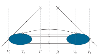
(a) general LCPT PDF graph

(b) corresponding LCPT DPD graph

Figure 1: transition from a given LCPT PDF graph to a corresponding LCPT DPD graph

$$2\left(\!x_{l}\,p^{+}\!\right)^{n_{l}}\mathcal{G}_{DPD}^{j_{1}j_{2}}=\mathcal{G}_{PDF}^{j_{1}}\,,$$ (4)

relating PDF and DPD graphs. Here $\mathcal{G}_{PDF}^{j_{1}}$ and $\mathcal{G}_{DPD}^{j_{1}j_{2}}$ are the LCPT expressions for a given PDF graph and one of its corresponding DPD graphs as illustrated in Fig. 1 while $x_{l}$ is understood to be the the longitudinal momentum fraction of the “cut” line in the same figure. With this the proof of the number sum rule reduces to showing the following

$$\sum_{l}\left(\delta_{f(l),\,j_{2}}-\delta_{f(l),\,\overline{j_{2}}}\right) =\left(N_{{j_{2}}_{v}}+\delta_{j_{1},\,\overline{j_{2}}}-\delta_{j_{1},\,j_{2}}\right)$$

$$\left(N\left(\vphantom{\overline{j_{2}}}j_{2}\right)_{\mathcal{G},\,c}-N\left(\overline{j_{2}}\right)_{\mathcal{G},\,c}\right) =\left(N_{{j_{2}}_{v}}+\delta_{j_{1},\,\overline{j_{2}}}-\delta_{j_{1},\,j_{2}}\right)\,.$$ (5)

In this expression $N\left(\vphantom{\overline{j_{2}}}j_{2}\right)$ and $N\left(\overline{j_{2}}\right)$ are the number of $j_{2}$ and $\overline{j_{2}}$ quarks respectively running over the final state cut in the considered PDF graph. I.e. in order to show the validity of the number sum rule we simply have to count the number of $j_{2}$ and $\overline{j_{2}}$ quarks. As for gluons the very notion of a valence DPD is ill defined the case $j_{2}=g$ can be neglected. Besides the $j_{2}$ valence quarks we find an arbitrary number, $x$, of $j_{2}\overline{j_{2}}$ pairs inside of a hadron. As these additional quarks however always come in pairs it is possible to express $N\left(\vphantom{\overline{j_{2}}}j_{2}\right)-N\left(\overline{j_{2}}\right)$ in terms of $j_{1}$, making the above equality evident. In order to show the validity of the momentum sum rule for bare distributions one has to show that the following equality holds

$$\sum_{l}\int\mathrm{D}_{2}^{N(t)}\left[x_{i}\right]\mathrm{D}_{1}^{N(t)}\left[\boldsymbol{k}_{i}\right]\,x_{l}\,\mathcal{G}^{j_{1}}\left(\{x\},\{\boldsymbol{k}\}\right)\delta\left(1-\textstyle{\sum_{i}}x_{i}\right)$$

$$= \left(1-x_{1}\right)\int\mathrm{D}_{2}^{N(t)}\left[x_{i}\right]\mathrm{D}_{1}^{N(t)}\left[\boldsymbol{k}_{i}\right]\mathcal{G}^{j_{1}}\left(\{x\},\{\boldsymbol{k}\}\right)\delta\left(1-\textstyle{\sum_{i}}x_{i}\right)\,,$$ (6)

where we used a shorthand notation for the integration measure

$$\int\mathrm{D}_{a}^{b}\left[x_{i}\right]=\prod_{i=a}^{b}\int_{0}^{1}\mathrm{d}x_{i}\,p^{+}\,, \int\mathrm{D}_{a}^{b}\left[\boldsymbol{k}_{i}\right]=\prod_{i=a}^{b}\int\frac{\mathrm{d}^{D-2}\boldsymbol{k}_{i}}{(2\pi)^{D-1}}\,.$$ (7)

This can however easily be shown by performing the $x_{2}$ integration using the momentum conservation $\delta$ function, yielding

$$\int\mathrm{D}_{3}^{N(t)}\left[x_{i}\right]\mathrm{D}_{1}^{N(t)}\left[\boldsymbol{k}_{i}\right]\left(1-x_{1}-\textstyle{\sum_{i\neq 2}}x_{i}+\textstyle{\sum_{l\neq 2}}x_{j}\right)\mathcal{G}^{j_{1}}\left(\{x\},\{\boldsymbol{k}\}\right)$$

$$= \left(1-x_{1}\right)\int\mathrm{D}_{3}^{N(t)}\left[x_{i}\right]\mathrm{D}_{1}^{N(t)}\left[\boldsymbol{k}_{i}\right]\mathcal{G}_{PDF_{c}}^{j_{1}}\left(\{x\},\{\boldsymbol{k}\}\right)\,.$$ (8)

At the level of bare distributions the analysis of LCPT graphs thus fully confirms the parton model intuition, leaving any possible violations of the sum rules to be due to renormalisation effects which we considered next.

3 Renormalisation

The renormalised distributions are obtained from the bare ones by a convolution with a PDF renormalisation $Z$ factor for each twist-2 operator in the matrix element defining the PDFs and DPDs. For the DPD in transverse momentum space one finds in addition to this furthermore an inhomogeneous term needed to renormalise the perturbative $1\to 2$ splitting, cf. section $3.2$ in Ref. 8.

$$\sum_{i_{1}}\!\!\int\limits_{x_{1}+x_{2}}^{1}\!\!\frac{\mathrm{d}z_{1}}{z_{1}^{2}}Z_{i_{1},j_{1}j_{2}}\left(\frac{x_{1}}{z_{1}},\frac{x_{2}}{z_{1}};\mu\right)f_{B}^{i_{1}}\left(z_{1}\right)\,.$$ (9)

In the minimal subtraction scheme the renormalisation factors are a series of pure poles in the dimensional parameter $\varepsilon$. In order to show the validity of the sum rules for renormalised quantities we subtract the r.h.s. of the respective sum rule from the l.h.s. and express the renormalised distributions in terms of bare ones convoluted with renormalisation factors. For the sum rules to hold this difference has so vanish. As both the l.h.s. and r.h.s. of the sum rules are finite for $\varepsilon\to 0$ (they involve renormalised quantities, after all) we can conclude that in the difference between both sides all poles in $\varepsilon$ have to cancel, leaving at most a finite difference. For both sum rules this difference can be brought to the following form

$$\sum_{i_{1}^{\prime}}\!\int\limits_{x_{1}}^{1}\!\frac{\mathrm{d}u_{1}}{u_{1}}f^{i_{1}^{\prime}}\left(u_{1};\mu\right)R\left(x_{1},u_{1};\mu\right)\,,$$ (10)

where $R\left(x_{1},u_{1};\mu\right)$ is a function of the renormalisation factors $Z$ and the only possible finite contribution is due to the tree-level term of the PDF renormalisation factors. One finds however that the tree level terms vanish explicitly. This argument can also be adapted to hold in the $\overline{\text{MS}}$ scheme. From the fact that $R$ in Eq. (10) vanishes we can furthermore obtain number and momentum sum rules for the $1\to 2$ renormalisation factor $Z_{i,jk}$, namely

$$\int\limits_{0}^{1-x_{1}}\!\!\!\mathrm{d}x_{2}\left(\!Z_{i,jk}\left(x_{i};\mu\right)-Z_{i,j\overline{k}}\left(x_{i};\mu\right)\!\right) =\left(\!\delta_{i,k}-\delta_{i,\overline{k}}+\delta_{j,\overline{k}}-\delta_{j,k}\!\right)\!Z_{i,j}\left(x_{1};\mu\right)\,,$$

$$\sum_{k}\!\!\int\limits_{0}^{1-x_{1}}\!\!\mathrm{d}x_{2}\,x_{2}\,Z_{i,jk}\left(x_{1},x_{2};\mu\right) =\left(1-x_{1}\right)Z_{i,j}\left(x_{1};\mu\right)\,.$$ (11)

4 Evolution

The consistency of the DPD sum rules with the LO evolution was already noted in Ref. 3. As we did not make any assumptions about the renormalisation scale $\mu$ in the proof of the sum rules they are valid for all values of $\mu$ implying their stability under QCD evolution to all orders. We furthermore generalised the double DGLAP (dDGLAP) equation[9, 10, 11, 12] to higher orders and checked that the result is consistent with the stability of the sum rules. We find that the inhomogeneous term becomes a convolution of a single PDF with a $1\to 2$ splitting kernel

$$\sum_{i_{1}}\int\limits_{x_{1}+x_{2}}^{1}\frac{\mathrm{d}v}{v^{2}}P_{i_{1},j_{1}j_{2}}\left(\frac{x_{1}}{v},\frac{x_{2}}{v}\right)f^{i_{1}}\left(v;\mu\right)\,,$$ (12)

where the higher order $1\to 2$ splitting kernel $P_{i,jk}$ is – in MS – given by

$$P_{i,jk}\left(x_{i};\alpha_{s}\left(\mu\right)\right)=-\alpha_{s}\left(\mu\right)\frac{\partial}{\partial\alpha_{s}}Z_{i,jk}^{(-1)}\left(x_{i},\alpha_{s}\left(\mu\right)\right)\,.$$ (13)

Here $Z_{i,jk}^{(-1)}$ is the coefficient of the ${}^{1}\!/\!{}_{\varepsilon}$ pole of $Z_{i,jk}$. Again, this can also be adapted to $\overline{\text{MS}}$. A first consistency check is that the renormalisation scale dependence of $Z_{i,jk}$ is also governed by the dDGLAP equation as one would expect. From this in combination with the sum rules for the $1\to 2$ renormalisation factor we furthermore derived analogous sum rules for the $1\to 2$ splitting kernels

$$\int\limits_{0}^{1-x_{1}}\!\!\!\mathrm{d}x_{2}\left(P_{i,jk}\left(x_{i}\right)-P_{i,j\overline{k}}\left(x_{i}\right)\right) =\left(\delta_{i,k}-\delta_{i,\overline{k}}+\delta_{j,\overline{k}}-\delta_{j,k}\right)P_{i,j}\left(x_{1}\right)\,,$$

$$\sum_{k}\!\!\int\limits_{0}^{1-x_{1}}\!\!\mathrm{d}x_{2}\,x_{2}\,P_{i,jk}\left(x_{i}\right) =\left(1-x_{1}\right)P_{i,j}\left(x_{1}\right)\,.$$ (14)

These sum rules provide a valuable cross check for future higher order calculations of the $1\to 2$ splitting kernels. We furthermore note that at LO the convolution in Eq. (12) can be performed trivially as the LO $1\to 2$ splitting kernel $P_{i_{1},j_{1}j_{2}}\left(x_{i}\right)$ is proportional to $\delta\left(1-x_{1}-x_{2}\right),$ reproducing the LO result[9, 10, 11, 12].

5 Perturbative splitting in DPDs

As already mentioned in section 1 perturbative splitting gives a sizeable contribution to the DPD for small interparton distance $y$ . In Ref. 8 an expression for this perturbative splitting contribution is given in Eq. $(3.14)$. Fourier transforming this expression to momentum space in $D-2$ dimensions we find that the ${}^{1}\!/\!{}_{y^{\ldots}}$ pole generates an additional ${}^{1}\!/\!{}_{\varepsilon}$ UV pole which has to be renormalised by the $Z_{i_{1},j_{1}j_{2}}$ factor appearing in Eq. (9). This is the actual origin of the inhomogeneous term in the renormalised DPD and in the dDGLAP equation. As $Z_{i_{1},j_{1}j_{2}}$ has to cancel the UV pole in the Fourier transformed splitting DPD their pole structure is closely related which makes it possible to calculate the $1\to 2$ splitting kernel $P_{i_{1},j_{1}j_{2}}$ from the $V_{i_{1},j_{1}j_{2}}$ kernel in Eq. $(3.15)$ in Ref. 8 using Eq. (13).

6 DPDs at $\boldsymbol{\Delta}=0$

An alternative way to regularise and renormalise the splitting singularity of the splitting DPD is to introduce a cut-off function $\Phi$ which can also be used to resolve the DPS SPS double counting issue[8].

$$F_{\Phi}^{j_{1}j_{2}}\left(x_{i},\boldsymbol{\Delta};\mu,\nu\right) =\int\mathrm{d}^{2}\boldsymbol{y}\,\mathrm{e}^{i\boldsymbol{y}\boldsymbol{\Delta}}\,\Phi\left(y\nu\right)F^{j_{1}j_{2}}\left(x_{i},\boldsymbol{y};\mu\right)\,.$$ (15)

As most calculations are performed in the modified minimal subtraction scheme a matching between the cut-off regularised DPD and the $\overline{\text{MS}}$ regularised version is needed. Due to the fact that $F_{\scriptscriptstyle\overline{\text{MS}}}^{j_{1}j_{2}}\left(x_{i},\boldsymbol{\Delta};\mu\right)$ and $F_{\Phi}^{j_{1}j_{2}}\left(x_{i},\boldsymbol{\Delta};\mu,\nu\right)$ differ only in how the UV divergence is regularised their difference can be calculated in perturbation theory and has the following form

$$\sum_{i_{1}}\!\int\limits_{x_{1}+x_{2}}^{1}\!\!\frac{\mathrm{d}v}{v^{2}}\,\,U_{i_{1},j_{1}j_{2}}\left(\frac{x_{i}}{v},\alpha_{s}\left(\mu\right),\log\left(\frac{\nu}{\mu}\right)\right)f^{i_{1}}\left(v;\mu\right)\,,$$ (16)

where the kernel $U_{i_{1},j_{1}j_{2}}$ can again be obtained from the $V_{i_{1},j_{1}j_{2}}$ kernel. To leading order in $\alpha_{s}$ this matching has already been derived in section 7 of Ref. 8. It should be noted that the $1\to 2$ splitting kernel there matches the one in this publication only to $\mathcal{O}(\alpha_{s})$ and for $\varepsilon=0$.

References

• 1. M. Rinaldi, S. Scopetta, M. C. Traini, and V. Vento, Correlations in Double Parton Distributions: Perturbative and Non-Perturbative effects, JHEP. 10, 063 (2016). 10.1007/JHEP10(2016)063. arXiv:1608.02521 [hep-ph].
• 2. F. A. Ceccopieri, M. Rinaldi, and S. Scopetta, Parton correlations in same-sign $W$ pair production via double parton scattering at the LHC (2017). arXiv:1702.05363 [hep-ph].
• 3. J. R. Gaunt and W. J. Stirling, Double Parton Distributions Incorporating Perturbative QCD Evolution and Momentum and Quark Number Sum Rules, JHEP. 03, 005 (2010). 10.1007/JHEP03(2010)005. arXiv:0910.4347 [hep-ph].
• 4. M. Diehl, P. Plößl, and A. Schäfer. DPD sum rules in QCD (2017). preprint in preparation.
• 5. B. Blok, Yu. Dokshitzer, L. Frankfurt, and M. Strikman, Perturbative QCD correlations in multi-parton collisions, Eur. Phys. J. C74, 2926 (2014). 10.1140/epjc/s10052-014-2926-z. arXiv:1306.3763 [hep-ph].
• 6. J. R. Gaunt. Double parton scattering in proton-proton collisions. PhD thesis, University of Cambridge (2012).
• 7. J. Collins, Foundations of perturbative QCD. Cambridge University Press (2013). ISBN 9781107645257, 9781107645257, 9780521855334, 9781139097826. URL http://www.cambridge.org/de/knowledge/isbn/item5756723.
• 8. M. Diehl, J. R. Gaunt, and K. Schönwald. Double hard scattering without double counting (2017). arXiv:1702.06486 [hep-ph].
• 9. V. P. Shelest, A. M. Snigirev, and G. M. Zinovev, The Multiparton Distribution Equations in QCD, Phys. Lett. B113, 325 (1982). 10.1016/0370-2693(82)90049-1.
• 10. V. Shelest, A. Snigirev, and G. Zinovjev, Gazing into the multiparton distribution equations in qcd, Physics Letters B. 113(4), 325 – 328 (1982). ISSN 0370-2693. http://dx.doi.org/10.1016/0370-2693(82)90049-1. URL http://www.sciencedirect.com/science/article/pii/0370269382900491.
• 11. F. A. Ceccopieri, An update on the evolution of double parton distributions, Phys. Lett. B697, 482–487 (2011). 10.1016/j.physletb.2011.02.047. arXiv:1011.6586 [hep-ph].
• 12. F. A. Ceccopieri, A second update on double parton distributions, Phys. Lett. B734, 79–85 (2014). 10.1016/j.physletb.2014.05.015. arXiv:1403.2167 [hep-ph].