How does light move in a generic metric-affine background?

Abstract

Light is the richest information retriever for most physical systems, particularly so for astronomy and cosmology, in which gravitation is of paramount importance, and also for solid state defects and metamaterials, in which some effects can be mimicked by non-Euclidean or even non-Riemannian geometries. Thus, it is expedient to probe light motion in geometrical backgrounds alternative to that of general relativity. Here we investigate this issue in generic metric-affine theories and derive (i) the expression, in the geometrical optics (eikonal) limit, for light trajectories, showing that they still are null (extremal) geodesics and thus, in general, no longer autoparallels, (ii) a generic formula to obtain the relation between source (galaxy) and reception (observer) angular size (area) distances, generalizing Etherington’s original distance reciprocity relation (DRR), and then applying it to two particular representative non-Riemannian geometries. First in metric-compatible, completely antisymmetric torsion geometries, the generalized DRR is not changed at all, and then in Weyl integrable spacetimes, the generalized DRR assumes a specially simple expression.

I Introduction

In 1933, at the culmination of a debate on relativistic distances, Etherington derived relations between two kinds of distance in an arbitrary Lorentzian geometry, the so-called distance reciprocity and duality relations *[][;republishedin]Etherington33; *Etherington07; Ellis (2007). This beautiful result, based on properties of null geodesics, lies at the heart of essentially all observations in astronomy and cosmology, and its refutation would be “a catastrophe from the theoretician’s viewpoint” Kristian and Sachs (1966) or “a major crisis for observational cosmology” Ellis (2007).

The usual distance reciprocity relation (DRR) connects the angular size distance, $D_{S}$, from an arbitrary instantaneous observer at the source to the angular size distance, $D_{R}$, from an arbitrary instantaneous observer at the reception (cf. Fig. 1). Its derivation is carried out by assuming, besides the Riemannian (in fact, Lorentzian) character of the spacetime, that there are neither interruption (absorption or creation) of light rays nor bifurcations (birefringence), and it reads $D_{S}=(1+z)\,D_{R}$, where $z$ is the redshift between the two instantaneous observers. If, furthermore, the energy-momentum tensor of the electromagnetic field is (covariantly) conserved (“photons are conserved”), then the so-called luminosity distance, $D_{L}$, may be related to $D_{S}$ so that we get Etherington’s famous usual distance duality relation (DDR): $D_{L}=(1+z)^{2}\,D_{R}$ . We remark that, in a cosmological (or even astronomical) setting, in general, none of the three distances are directly measurable; we always have to assume or derive the value of some proper feature of the inaccessible source (emission beam solid angle, transverse area or luminosity). To investigate a possible violation of this canonical DDR, it is expedient to define

$$\eta:=\dfrac{D_{L}}{(1+z)^{2}D_{R}}\,.$$ (1)

For general relativity (GR), of course $\eta=1$. Observational constraints on its value have been extensively explored in the recent literature Bassett and Kunz (2004); Uzan et al. (2004); More et al. (2009); Avgoustidis et al. (2010); Khedekar and Chakraborti (2011); Lima et al. (2011); Nair et al. (2011); Cardone et al. (2012); Holanda et al. (2012); Nair et al. (2012); Ellis et al. (2013); Yang et al. (2013); Santos-da-Costa et al. (2015); Liao et al. (2015); Wu et al. (2015); Avgoustidis et al. (2016); Räsänen et al. (2016).

Light is an electromagnetic phenomenon and thus its trajectories, in the geometrical optics or eikonal (high frequency, nearly monochromatic plane wave) approximation, should be suitably derived from Maxwell’s equations in a convenient background. Both in the special relativistic context and in GR as well, this leads to the well-known and pleasing result that light moves on null (extremal, metric) geodesics (or autoparallels or affine geodesics, which do coincide with the metric geodesics in a Riemannian geometry) Born and Wolf (1999); Schneider et al. (1992). However, there are many alternative theories of gravity or even effective field theories (for metamaterials or solid state physics), which are built on top of more general non-Riemannian geometries. We will be particularly interested in those where, in contrast to Einstein’s GR, the affine connection has nonvanishing torsion and nonmetricity (to be defined in the next section); for general reviews and motivation, see Hehl et al. (1995); Hammond (2002); Shapiro (2002); Ni (2010); Vitagliano (2014). This is a sufficiently wide class of theories to include: Einstein-Cartan theory Hehl et al. (1976), teleparallel theories Aldrovandi and Pereira (2013), Weyl theories Scholz (2017), metric-affine gauge theories Hehl et al. (1995), Kalb-Ramond string fields Mukhopadhyaya et al. (2002); Das et al. (2014), metamaterials Horsley (2011) and to also incorporate a generalized Ehlers-Pirani-Schild approach for chronogeometry Ehlers et al. (1972).

Our aim is twofold: to derive, under the scope of a completely general metric-affine geometry, (i) the trajectories light follows and, therefrom, (ii) the generalized DRR. As an application, we employ it to two particular non-Riemannian geometries.

II General metric-affine background

The class of theories we envisage are those which have a metric-affine background, constituted by any model $({\mathcal{M}},g_{\alpha\beta},{\Gamma^{\alpha}}_{\mu\nu})$, where ${\mathcal{M}}$ is the base manifold, $g_{\alpha\beta}$ is a Lorentzian metric tensor (with signature $+2$) and ${\Gamma^{\alpha}}_{\mu\nu}$ is a generic (asymmetric) affine connection, such that, in general, the corresponding torsion and nonmetricity tensors are defined respectively by

$${T^{\alpha}}_{\mu\nu} :=2{\Gamma^{\alpha}}_{[\mu\nu]}\,,$$ (2)

$$Q_{\alpha\beta\gamma} :=\nabla_{\gamma}g_{\alpha\beta}\,,$$ (3)

where, of course, $\nabla$ stands for the covariant derivative with respect to the fundamental connection $\Gamma$, whereas, later on, $\widehat{\nabla}$ will stand for the covariant derivative with respect to the (auxiliary) Levi-Civita connection $\widehat{\Gamma}$. These connections are related by a useful identity Schouten (1954):

$${\Gamma^{\alpha}}_{\mu\nu}={{\widehat{\Gamma}}^{\alpha}}_{\ \,\mu\nu}+{\Delta^{\alpha}}_{\mu\nu}\,,$$ (4)

where

$${\widehat{\Gamma}}\indices :=\left\{{}\indices{{}_{\mu}}\!{}\indices{{}^{\alpha}}{}\!\indices{{}_{\nu}}\right\}:=\dfrac{1}{2}g^{\alpha\beta}{\left(\partial_{\nu}g_{\beta\mu}+\partial_{\mu}g_{\beta\nu}-\partial_{\beta}g_{\mu\nu}\right)}\,,$$ (5)

$${\Delta^{\alpha}}_{\mu\nu} :={K^{\alpha}}_{\mu\nu}+{D^{\alpha}}_{\mu\nu}\,,$$ (6)

and

$${K^{\alpha}}_{\mu\nu} :=\dfrac{1}{2}\left({T_{\mu\nu}}^{\alpha}+{T_{\nu\mu}}^{\alpha}+{T^{\alpha}}_{\mu\nu}\right)\,,$$ (7)

$${D^{\alpha}}_{\mu\nu} :=\dfrac{1}{2}\left(Q\indices{{}_{\mu\nu}^{\alpha}}-Q\indices{{}^{\alpha}_{\mu\nu}}-Q\indices{{}_{\nu}^{\alpha}{}_{\mu}}\right)\,.$$ (8)

Here $\left\{{}\indices{{}_{\mu}}\!{}\indices{{}^{\alpha}}{}\!\indices{{}_{\nu}}\right\}$ is the Christoffel symbol (of the second kind), $K\indices{{}^{\alpha}_{\mu\nu}}$ is the contortion tensor and $D\indices{{}^{\alpha}_{\mu\nu}}$ is the deflection tensor. Of course, the usual Lorentzian case, which includes GR and all $f(R)$ theories, corresponds to ${T^{\alpha}}_{\mu\nu}=Q_{\alpha\beta\mu}=0$ , whence ${\Gamma^{\alpha}}_{\mu\nu}={\widehat{\Gamma}}\indices{{}^{\alpha}_{\mu\nu}}$ . Our results are independent of any specific form for the governing equations of the fundamental gravitational fields, which, without any loss of generality, will be taken as ${\boldsymbol{\mathcal{G}}}:=(g\indices{{}_{\alpha\beta}},T\indices{{}^{\alpha}_{\mu\nu}},Q\indices{{}_{\alpha\beta\gamma}})$ .

III Geometrical optics approximation

There are several classical approaches aiming to derive the trajectories followed by light, in the geometrical optics or eikonal approximation: asymptotic series Ehlers (1967); Misner et al. (1973); Schneider et al. (1992); Perlick (2000); Bóna and Slawinski (2011), Fourier transform Born and Wolf (1999); Horsley (2011) and characteristics or discontinuities Courant and Hilbert (1989); Kline and Kay (1965); Born and Wolf (1999); Friedlander (1975); Bóna and Slawinski (2011).

Here we follow the asymptotic series one and, therefore, we only have to impose conditions on the higher-order derivative terms (the principal part) for the generalized vacuum Maxwell equations, in the absence of sources, of the antisymmetric electromagnetic field tensor, $F\indices{{}_{\alpha\beta}}$. Inspired by the usual case, we assume they are still two sets of first-order (in $F\indices{{}_{\alpha\beta}}$) linear homogeneous partial differential equations given by

$$\left[\nabla_{\beta}+\chi_{\beta}({\boldsymbol{\mathcal{G}}},\nabla{\boldsymbol{\mathcal{G}}},\ldots)\right]F^{\alpha\beta} =0\,,$$ (9)

$$\left[\nabla_{[\alpha}+\zeta_{[\alpha}({\boldsymbol{\mathcal{G}}},\nabla{\boldsymbol{\mathcal{G}}},\ldots)\right]F_{\beta\gamma]} =0\,.$$ (10)

Here $\chi_{\alpha}$ and $\zeta_{\alpha}$ are arbitrary covariant vector fields dependent only on ${\boldsymbol{\mathcal{G}}}$ and their (covariant) derivatives up to a finite order. Constraints on their expressions might be established either from additional physical assumptions, such as the existence of a 4-potential or charge conservation, or from a variational approach. Of course, the existence of a 4-potential will impose, through Poincaré’s lemma, a constraint on $\zeta_{\alpha}$ whereas charge conservation will restrict $\chi_{\alpha}$, from Eq. (9) with a source term. Hence, if one wants to ensure both, one does not necessarily need to postulate the usual set of Maxwell equations of GR, neither a Riemannian background.

Resuming now our main derivation, we look for (asymptotic) solutions of the generalized Maxwell equations (9) and (10) in the form of a monochromatic wave:

$$F_{\mu\nu}=\Re\,{[A_{\mu\nu}(x)e^{iS(x)/\epsilon}]},$$ (11)

where $A_{\mu\nu}$ is an antisymmetric tensor field, $S$ is a real scalar field, the phase of the wave, $\epsilon$ is a control parameter for the wavelength, and $\Re$ indicates that the real part of the following expression is to be taken.

Inserting Eq. (11) into Eqs. (9) and (10), and imposing the condition $\epsilon\rightarrow 0$, we obtain

$$k^{\mu}k_{\mu}=0,\hskip 28.45274ptk_{\mu}:=\partial_{\mu}S,$$ (12)

where $k_{\mu}$ is the wave 4-vector, whose integral curves are to be considered as the light rays. This condition is completely independent of $\chi_{\alpha}$ and $\zeta_{\alpha}$. From Eq. (12), we immediately derive our first simple general result, valid for any metric-affine theory and linear generalized Maxwell’s equations: the light rays are (extremal) metric geodesics ($k^{\nu}\widehat{\nabla}_{\nu}k^{\mu}=0\,$), as in GR, although, in general, no longer affine geodesics (autoparallels),

$$\accentset{\mbox{\large.}}{k}^{\mu}=[T_{\alpha\beta}^{\hskip 8.5359pt\mu}+(1/2)Q_{\alpha\beta}^{\hskip 11.38092pt\mu}-Q^{\mu}_{\hskip 5.69046pt\alpha\beta}]k^{\alpha}k^{\beta}\,,$$ (13)

in contrast to GR. Here and later on $\accentset{\mbox{\large.}}{Z}^{\alpha\cdots}_{\hskip 11.38092pt\beta\cdots}\!\!:=k^{\nu}\nabla_{\nu}Z^{\alpha\cdots}_{\hskip 11.38092pt\beta\cdots}$ .

In addition, completing the geometrical optics limit, we were able to obtain evolution equations for the scalar amplitude as well as the polarization of the electromagnetic wave, showing that both quantities are parallely propagated along the light rays, although the family of such quantities satisfying such conditions is dependent on the choice of $\chi_{\alpha}$ and $\zeta_{\alpha}$.

IV Generalized distance reciprocity relation

Now, from Eq. (13), we derive our second general result: for any metric-affine geometry, the generalized deviation equation for the light rays is

$$\accentset{\mbox{\large..}}{X}^{\alpha}={R^{\alpha}}_{\mu\nu\sigma}k^{\mu}k^{\nu}X^{\sigma}+X^{\nu}\nabla_{\nu}\accentset{\mbox{\large.}}{k}^{\alpha}-({T^{\alpha}}_{\mu\nu}k^{\mu}X^{\nu})\!\accentset{\mbox{\large.}}{\phantom{x}},$$ (14)

where $X^{\alpha}$ is any connecting vector field associated to a congruence of light rays. We stress that this result turns out to coincide with the one in Swaminarayan and Safko (1983), but there it was proven only for the particular case of vanishing nonmetricity.

Next, let $\mathcal{B}_{i}$, $i=\mathcal{S},\mathcal{R}$, be two 2-parameter infinitesimal pencil beams of generalized light rays, such that their vertices are the events $i=\mathcal{S}$ (for source) and $i=\mathcal{R}$ (for reception), along a single common curve, the so-called fiducial light ray $\mathcal{C}$.

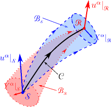
Figure 1: Spacetime diagram for the infinitesimal light beams $\mathcal{B}_{{}_{\mathcal{S}}}$ (dashed) and $\mathcal{B}_{{}_{\mathcal{R}}}$ (dotted) based, respectively, at events source $\mathcal{S}$ and reception $\mathcal{R}$, their common fiducial light ray $\mathcal{C}$ (solid), and the corresponding connecting vectors $\left.X^{\alpha}\right|_{\mathcal{R}}$ and $\left.Y^{\alpha}\right|_{\mathcal{S}}$.

In the Riemmanian case, if $X^{\mu}$ and $Y^{\mu}$ are the connecting vector fields of $\mathcal{B}_{R}$ and $\mathcal{B}_{S}$, respectively, there is a conserved quantity along the fiducial light ray, namely,

$$Y_{\mu}\accentset{\mbox{\large.}}{X}^{\mu}-X_{\mu}\accentset{\mbox{\large.}}{Y}^{\mu}=\text{constant along }\mathcal{C}.$$ (15)

Given any pair of connecting vectors of $\mathcal{B}_{{}_{\mathcal{S}}}$ ($X^{\mu}$ and $\tilde{X}^{\mu}$), and any pair of connecting vectors of $\mathcal{B}_{{}_{\mathcal{R}}}$ ($Y^{\mu}$ and $\tilde{Y}^{\mu}$), from Eq. (15)

$$\left.\left(Y_{\mu}\accentset{\mbox{\large.}}{X}^{\mu}\right)\right|_{\mathcal{S}}\left.\left(\tilde{Y}_{\nu}\accentset{\mbox{\large.}}{\tilde{X}}^{\nu}\right)\right|_{\mathcal{S}}=\left.\left(X_{\mu}\accentset{\mbox{\large.}}{Y}^{\mu}\right)\right|_{\mathcal{R}}\left.\left(\tilde{X}_{\nu}\accentset{\mbox{\large.}}{\tilde{Y}}^{\nu}\right)\right|_{\mathcal{R}}.$$ (16)

Provided that $X^{\mu}$ and $\tilde{X}^{\mu}$ are a pair of orthogonal connecting vector fields of $\mathcal{B}_{{}_{\mathcal{S}}}$, belonging to the screen space of $\left.u^{\alpha}\right|_{\mathcal{R}}$, $Y^{\mu}$ and $\tilde{Y}^{\mu}$, a pair of orthogonal connecting vector fields of $\mathcal{B}_{{}_{\mathcal{R}}}$, belonging to the screen space of $\left.u^{\alpha}\right|_{\mathcal{S}}$, the usual DRR, which holds for arbitrary Lorentzian spacetimes, is essentially equivalent to Ellis (1971); Plebański and Krasiński (2006) (notice however the different notation)

$$dA_{\mathcal{S}}\,d\Omega_{\mathcal{S}}\!\left.(k_{\mu}u^{\mu})^{2}\right|_{\mathcal{S}}=dA_{\mathcal{R}}\,d\Omega_{\mathcal{R}}\!\left.(k_{\mu}u^{\mu})^{2}\right|_{\mathcal{R}}\,,$$ (17)

where $dA_{\mathcal{S},\mathcal{R}}$ is an infinitesimal area of the beam $\mathcal{B}_{\mathcal{R},\mathcal{S}}$ and $d\Omega_{\mathcal{R},\mathcal{S}}$ is the corresponding infinitesimal solid angle, both with respect to the instantaneous observer at the event given by the subindex (cf. Fig. 1) .

When reading the classical works on this subject Ellis (1971); Plebański and Krasiński (2006), one might be tempted to think that Eq. (15) is a necessary result for the imposition of the previous conditions on the connecting vectors. We, however, follow a different approach, treating the previous constraints on those vectors simply as the initial conditions for their respective set of deviation equations [cf. (14)]. Thus, we see Eq. (15) as a means to relate cosmological observables in $\mathcal{S}$ to their respective counterparts in $\mathcal{R}$.

Now, from the usual definitions of redshift, $1+z:=\left.(k_{\mu}u^{\mu})\right|_{\mathcal{S}}/\left.(k_{\mu}u^{\mu})\right|_{\mathcal{R}}$ , and the angular size distances, $D_{S,R}:=\sqrt{dA_{\mathcal{R},\mathcal{S}}/d\Omega_{\mathcal{S},\mathcal{R}}}$ , we immediately have

$$D_{S}=(1+z)D_{R}\,.$$ (18)

In a generic metric-affine theory, Eq. (16) is replaced instead by

$$\begin{split}&\left.\left(Y_{\mu}\accentset{\mbox{\large.}}{X}^{\mu}\right)\right|_{\mathcal{S}}\left.\left(\tilde{Y}_{\nu}\accentset{\mbox{\large.}}{\tilde{X}}^{\nu}\right)\right|_{\mathcal{S}}=\left.\left(X_{\mu}\accentset{\mbox{\large.}}{Y}^{\mu}\right)\right|_{\mathcal{R}}\left.\left(\tilde{X}_{\nu}\accentset{\mbox{\large.}}{\tilde{Y}}^{\nu}\right)\right|_{\mathcal{R}}+\\ &\frac{1}{2}\left[\big{(}\left.Y_{\rho}\accentset{\mbox{\large.}}{X}^{\rho}\right|_{\mathcal{S}}-\left.X_{\rho}\accentset{\mbox{\large.}}{Y}^{\rho}\right|_{\mathcal{R}}\big{)}\tilde{\mathcal{I}}+\big{(}\left.\tilde{Y}_{\rho}\accentset{\mbox{\large.}}{\tilde{X}}^{\rho}\right|_{\mathcal{S}}-\left.\tilde{X}_{\rho}\accentset{\mbox{\large.}}{\tilde{Y}}^{\rho}\right|_{\mathcal{R}}\big{)}\mathcal{I}\right]\,.\end{split}$$ (19)

Here $\mathcal{I}$ and $\tilde{\mathcal{I}}$ stand for the functionals

$$\mathcal{I} :=\int_{\mathcal{C}_{\mathcal{S}\to\mathcal{R}}}M({\boldsymbol{\mathcal{G}}},k^{\alpha},X^{\alpha},Y^{\alpha})\,d\vartheta,$$ (20)

$$\tilde{\mathcal{I}} :=\int_{\mathcal{C}_{\mathcal{S}\to\mathcal{R}}}M({\boldsymbol{\mathcal{G}}},k^{\alpha},\tilde{X}^{\alpha},\tilde{Y}^{\alpha})\,d\vartheta,$$ (21)

where $\vartheta$ is a parameter along the fiducial light ray, and

$$\begin{split}M:=&\left[Q_{\sigma\mu[\nu;\rho]}+Q_{\mu\rho[\sigma;\nu]}+Q_{\mu\nu[\sigma;\rho]}+Q_{\sigma\rho[\mu;\nu]}+Q_{\sigma\nu[\rho;\mu]}+T^{\lambda}_{\hskip 5.69046pt\nu[\rho}Q_{\mu]\sigma\lambda}+T^{\lambda}_{\hskip 5.69046pt\sigma[\nu}Q_{\rho]\mu\lambda}+T^{\lambda}_{\hskip 5.69046pt\mu[\sigma}Q_{\rho]\nu\lambda}+T^{\lambda}_{\hskip 5.69046pt\nu\rho;(\sigma}g_{\mu)\lambda}+\right.\\ &\left.T^{\lambda}_{\hskip 5.69046pt\nu\rho}T_{(\sigma\mu)\lambda}+2g_{\lambda(\sigma}T^{\lambda}_{\hskip 5.69046pt\mu)[\nu;\rho]}+2T^{\lambda}_{\hskip 5.69046pt[\nu|(\sigma}T_{\mu)\lambda|\rho]}\right]Y^{\rho}k^{\sigma}k^{\mu}X^{\nu}+X_{\rho}({T^{\rho}}_{\mu\nu}k^{\mu}Y^{\nu})\!\accentset{\mbox{\large.}}{\phantom{x}}-Y_{\rho}({T^{\rho}}_{\mu\nu}k^{\mu}X^{\nu})\!\accentset{\mbox{\large.}}{\phantom{x}}+\accentset{\mbox{\large.}}{Y}_{\rho}\accentset{\mbox{\large.}}{X}^{\rho}-\\ &\accentset{\mbox{\large.}}{X}_{\rho}\accentset{\mbox{\large.}}{Y}^{\rho}+(X^{\mu}Y_{\nu}-Y^{\mu}X_{\nu})(\accentset{\mbox{\large.}}{k}^{\nu})_{;\mu}.\end{split}$$ (22)

Here for brevity $Z^{\alpha\cdots}_{\hskip 11.38092pt\beta\cdots;\mu}:=\nabla_{\mu}Z^{\alpha\cdots}_{\hskip 11.38092pt\beta\cdots}$.

We can rearrange Eq. (19) (cf. the comments before Eq. (17) and Eq. (18)) in order to obtain a generalization of the usual DRR, viz.:

$$D_{S}=(1+z)D_{R}\big{(}1+\mathcal{J}\big{)}^{1/2}\,,$$ (23)

where

$$\mathcal{J}:=-\frac{\big{(}\left.Y_{\rho}\accentset{\mbox{\large.}}{X}^{\rho}\right|_{\mathcal{S}}-\left.X_{\rho}\accentset{\mbox{\large.}}{Y}^{\rho}\right|_{\mathcal{R}}\big{)}\tilde{\mathcal{I}}+\big{(}\left.\tilde{Y}_{\rho}\accentset{\mbox{\large.}}{\tilde{X}}^{\rho}\right|_{\mathcal{S}}-\left.\tilde{X}_{\rho}\accentset{\mbox{\large.}}{\tilde{Y}}^{\rho}\right|_{\mathcal{R}}\big{)}\mathcal{I}}{2\left.\left(Y_{\mu}\accentset{\mbox{\large.}}{X}^{\mu}\right)\right|_{\mathcal{S}}\left.\left(\tilde{Y}_{\nu}\accentset{\mbox{\large.}}{\tilde{X}}^{\nu}\right)\right|_{\mathcal{S}}}.$$ (24)

This gives a definite procedure to obtain corrections of the usual distance reciprocity relation due to modified electrodynamics or gravitation, and provides a theoretical grounding for the phenomenological parameterizations in the literature.

Equations (19) to (24) allow us to calculate $\mathcal{J}$ regardless of the gravitational field equations or the full form of the sourceless electromagnetic ones, as long as they can be written as Eqs. (9) and (10). Of course $\mathcal{J}$ vanishes for GR (in fact for any Riemannian geometry). Despite the general form which the functional $\mathcal{J}$ may assume, we apply, in the next section, the result in Eq. (23) to two simple non-Riemannian geometries and discuss their most prominent consequences.

V Application: two simple cases

Now we apply the generalized DRR formula in Eq. (23) to a couple of simple non-Riemannian geometries. First, let us consider a metric connection ($Q_{\alpha\beta\mu}=0$) whose torsion is completely antisymmetric ($T_{\alpha\beta\mu}=-T_{\beta\alpha\mu}\Rightarrow T_{[\alpha\beta\mu]}=T_{\alpha\beta\mu}$) . This does not necessarily imply the connection is the Levi-Civita one. However it does imply, through Eq. (13), that light rays follow both affine geodesics (autoparallels) as well as (extremal) metric geodesics. This is just the content of the weak equivalence principle, at least for nonmassive particles. Moreover, it is straightforward to show that $\mathcal{J}$ vanishes, and the usual DRR of Riemannian geometry is preserved in the form of Eq. (18). In other words, we have shown that Riemannian geometry is a sufficient condition for the validity of the usual DRR, but not a necessary one.

The second case we consider is the Weyl integrable spacetime (WIST) nonmetric ($Q_{\mu\nu\lambda}\neq 0$) symmetric ($T^{\lambda}_{\hskip 5.69046pt\mu\nu}=0$) connection: $Q_{\mu\nu\lambda}=g_{\mu\nu}\partial_{\lambda}\phi$, where $\phi$ is a completely arbitrary real scalar field. These conditions imply again that light rays follow both affine and metric geodesics, although their affine parameters now differ. Furthermore, we have shown that $\mathcal{J}=e^{2(\phi|_{\mathcal{R}}-\phi|_{\mathcal{S}})}-1$ , and the DRR can now be cast in the following form:

$$D_{S}=(1+z)D_{R}e^{(\phi|_{\mathcal{R}}-\phi|_{\mathcal{S}})}\,.$$ (25)

This shows that a convenient choice of the WIST scalar field Santana et al. will provide a derivation of the phenomenological modifications of the usual DRR (or DDR; cf. below), ordinarily assumed in a vast class of recent works Bassett and Kunz (2004); Lima et al. (2011); Nair et al. (2011); Holanda et al. (2012); Wu et al. (2015).

VI Conclusion

In this work we focused on the influence of the geometrical structure of spacetime on electromagnetic phenomena, namely, light trajectories in the geometrical optics approximation and the distance reciprocity relation, both in generalized metric-affine theories.

We have shown that light rays still follow metric geodesics, as in GR, although those curves are no longer autoparallels when considering nonvanishing torsion and nonmetricity. This result holds for any set of partial linear homogeneous differential equations for the electromagnetic field [cf. Eqs. (9) and (10)]. Naturally, if one wishes to ensure the usual symmetries of electromagnetism, such as charge conservation, or existence of four-potential (gauge symmetry), this would imply constraints on $\chi_{\alpha}$ and $\zeta_{\alpha}$ [cf. the comments after Eqs. (9) and (10)].

We also obtained that the deviation equation (14) holds for a more general context, one with arbitrary nonmetricity. Using the previous result, we were able to exhibit the modifications of DRR in the presence of torsion and nonmetricity, providing two simple cases as an application. We emphasize that these results are completely independent of the field equations for gravitation.

To obtain a generalized DDR from our DRR, Eq. (19), based solely on the arbitrary metric-affine background and our reasonably general, but unspecified, Maxwell’s equations (9) and (10), does not seem feasible, unless we postulate a conservation of “photon number.” If we do so, then it is straightforward to show that the parameter $\eta$ from Eq. (1) is related to the functional $\mathcal{J}$ from Eq. (19) as $\eta^{2}=1+{\mathcal{J}}$ . In general, however, it is physically transparent that, due to the arbitrariness of the interaction between the gravitational fields and the electromagnetic one, the most we can hope for is a balance equation for photon number Calvão et al. (1992); alternatively, we do not have an explicit expression for the electromagnetic energy-momentum tensor field. To establish such a generalized balance equation for the photon number one might proceed in three distinct ways: to choose an electromagnetic Lagrangian or explicit expressions for $\chi_{\alpha}$ and $\zeta_{\alpha}$, to follow a thermodynamic approach Calvão et al. (1992), or to deal with a kinetic treatment Lima and Baranov (2014). We tackle this issue in a future investigation where observational constraints on specific models are explored as well.

References

- Etherington (1933) I. M. H. Etherington, “On the definition of distance in general relativity,” Philos. Mag. Ser. 7 15, 761 (1933).
- Etherington (2007) I. M. H. Etherington, “Republication of: LX. On the definition of distance in general relativity,” Gen. Relativ. Gravit. 39, 1055 (2007).
- Ellis (2007) G F. R. Ellis, “On the definition of distance in general: I. M. H. Etherington (Philosophical Magazine ser. 7, vol. 15, 761 (1933)),” Gen. Relativ. Gravit. 39, 1047 (2007).
- Kristian and Sachs (1966) J. Kristian and R. K. Sachs, “Observations in cosmology,” Astrophys. J. 143, 379 (1966).
- Bassett and Kunz (2004) B. A. Bassett and M. Kunz, “Cosmic distance-duality as a probe of exotic physics and acceleration,” Phys. Rev. D 69, 101305 (2004).
- Uzan et al. (2004) J.-P Uzan, N. Aghanim, and Y. Mellier, “Distance duality relation from x-ray and Sunyaev-Zel’dovich observations of clusters,” Phys. Rev. D 70, 083533 (2004).
- More et al. (2009) S. More, J. Bovy, and D. W. Hogg, “Cosmic transparency: A test with the baryon acoustic feature and type Ia supernovae,” Astrophys. J. 696, 1727 (2009).
- Avgoustidis et al. (2010) A. Avgoustidis, C. Burrage, J. Redondo, L. Verde, and R. Jimenez, “Constraints on cosmic opacity and beyond the standard model physics from cosmological distance measurements,” J. Cosmol. Astropart. Phys. 10, 024 (2010).
- Khedekar and Chakraborti (2011) S. Khedekar and S. Chakraborti, “A new Tolman test of a cosmic distance duality relation at 21 cm,” Phys. Rev. Lett. 106, 221301 (2011).
- Lima et al. (2011) J. A. S. Lima, J. V. Cunha, and V. T. Zanchin, “Deformed distance duality relations and supernova dimming,” Astrophys. J. Lett. 742, L26 (2011).
- Nair et al. (2011) R. Nair, S. Jhingan, and D. Jain, “Observational cosmology and the cosmic distance duality relation,” J. Cosmol. Astropart. Phys. 05, 023 (2011).
- Cardone et al. (2012) V. F. Cardone, S. Spiro, I. Hook, and R. Scaramella, “Testing the distance duality relation with present and future data,” Phys. Rev. D 85, 123510 (2012).
- Holanda et al. (2012) R. F. L. Holanda, J. A. S. Lima, and M. B. Ribeiro, “Probing the cosmic distance-duality relation with the Sunyaev-Zel’dovich effect, X-ray observations and supernovae Ia,” Astron. Astrophys. 538, A131 (2012).
- Nair et al. (2012) R. Nair, S. Jhingan, and D. Jain, “Cosmic distance duality and cosmic transparency,” J. Cosmol. Astropart. Phys. 12, 028 (2012).
- Ellis et al. (2013) G. F. R. Ellis, R. Poltis, J.-P. Uzan, and A. Weltman, “Blackness of the cosmic microwave background spectrum as a probe of the distance-duality relation,” Phys. Rev. D 87, 103530 (2013).
- Yang et al. (2013) X. Yang, H.-R. Yu, and T.-J. Zhang, “Constraining smoothness parameter and the DD relation of Dyer-Roeder equation with supernovae,” J. Cosmol. Astropart. Phys. 06, 007 (2013).
- Santos-da-Costa et al. (2015) S. Santos-da-Costa, V. C. Busti, and R. F.L. Holanda, “Two new tests to the distance duality relation with galaxy clusters,” J. Cosmol. Astropart. Phys. 10, 061 (2015).
- Liao et al. (2015) K. Liao, A. Avgoustidis, and Z. Li, “Is the Universe transparent?” Phys. Rev. D 92, 123539 (2015).
- Wu et al. (2015) P. Wu, Z. Li, X. Liu, and H. Yu, “Cosmic distance-duality relation test using type Ia supernovae and the baryon acoustic oscillation,” Phys. Rev. D 92, 023520 (2015).
- Avgoustidis et al. (2016) A. Avgoustidis, R. T. Génova-Santos, G. Luzzi, and C. J. A. P. Martins, “Subpercent constraints on the cosmological temperature evolution,” Phys. Rev. D 93, 043521 (2016).
- Räsänen et al. (2016) S. Räsänen, J. Väliviita, and V. Kosonen, “Testing distance duality with CMB anisotropies,” J. Cosmol. Astropart. Phys. 04, 050 (2016).
- Born and Wolf (1999) M. Born and E. Wolf, Principles of Optics. Electromagnetic Theory of Propagation, Interference and Diffraction of Light, 7th ed. (Cambridge University Press, Cambridge, 1999).
- Schneider et al. (1992) P. Schneider, J. Ehlers, and E. E. Falco, Gravitational Lenses (Springer-Verlag, Berlin, 1992).
- Hehl et al. (1995) F. W. Hehl, J. D. McCrea, E. W. Mielke, and Y. Ne’eman, “Metric-affine gauge theory of gravity: field equations, Noether identities, world spinors, and breaking of dilation invariance,” Phys. Rep. 258, 1 (1995).
- Hammond (2002) R. T. Hammond, “Torsion gravity,” Rep. Prog. Phys. 65, 599 (2002).
- Shapiro (2002) I. L. Shapiro, “Physical aspects of the space-time torsion,” Phys. Rep. 357, 113 (2002).
- Ni (2010) W.-T. Ni, “Searches for the role of spin and polarization in gravity,” Rep. Prog. Phys. 73, 056901 (2010).
- Vitagliano (2014) V. Vitagliano, “The role of nonmetricity in metric-affine theories of gravity,” Classical Quantum Gravity 31, 045006 (2014).
- Hehl et al. (1976) F. W. Hehl, P. von der Heyde, G. D. Kerlick, and J. M. Nester, “General relativity with spin and torsion: Foundations and prospects,” Rev. Mod. Phys. 48, 393 (1976).
- Aldrovandi and Pereira (2013) R. Aldrovandi and J. G. Pereira, Teleparallel Gravity (Springer, Dordrecht, 2013).
- Scholz (2017) E. Scholz, “Paving the way for transitions — a case for Weyl geometry,” in Towards a Theory of Spacetime Theories. Einstein Studies, Vol. 13., edited by D. Lehmkuhl, G. Schiemann, and E. Scholz (Birkhäuser, New York, 2017) p. 171.
- Mukhopadhyaya et al. (2002) B. Mukhopadhyaya, S. Sen, and S. SenGupta, “Does a Randall-Sundrum scenario create the illusion of a torsion-free universe?” Phys. Rev. Lett. 89, 121101 (2002).
- Das et al. (2014) A. Das, B. Mukhopadhyaya, and S. SenGupta, “Why has spacetime torsion such negligible effect on the Universe?” Phys. Rev. D 90, 107901 (2014).
- Horsley (2011) S. A. R. Horsley, “Transformation optics, isotropic chiral media and non-riemannian geometry,” New J. Phys. 13, 053053 (2011).
- Ehlers et al. (1972) J. Ehlers, F.. A. E. Pirani, and A. Schild, “The geometry of free fall and light propagation,” in General Relativity. Papers in Honour of J. L. Synge, edited by L. O’Raifeartaigh (Oxford University Press, Oxford, 1972) Chap. 4, p. 63.
- Schouten (1954) J. A. Schouten, Ricci-Calculus, 2nd ed. (Springer-Verlag, Berlin, 1954).
- Ehlers (1967) J. Ehlers, “Zum Übergang von der Wellenoptik zur geometrischen Optik in der allgemeinen Relativitätstheorie,” Z. Naturforsch. 22a, 1328 (1967).
- Misner et al. (1973) C. W. Misner, K. S. Thorne, and J. A. Wheeler, Gravitation (Freeman, San Francisco, 1973).
- Perlick (2000) V. Perlick, Ray Optics, Fermat’s Principle, and Applications to General Relativity (Springer-Verlag, Berlin, 2000).
- Bóna and Slawinski (2011) A. Bóna and M. A. Slawinski, Wavefronts and Rays as Characteristics and Asymptotics (World Scientific, Singapore, 2011).
- Courant and Hilbert (1989) R. Courant and D. Hilbert, Methods of Mathematical Physics, 2nd ed. (Wiley-VCH, Berlin, 1989).
- Kline and Kay (1965) M. Kline and I. W. Kay, Electromagnetic Theory and Geometrical Optics (John Wiley & Sons, New York, 1965).
- Friedlander (1975) F. G. Friedlander, The Wave Equation on a Curved Space-Time (Cambridge University Press, Cambridge, 1975).
- Swaminarayan and Safko (1983) N. S. Swaminarayan and J. L. Safko, “A coordinate-free derivation of a generalized geodesic deviation equation,” J. Math. Phys. 24, 883 (1983).
- Ellis (1971) G. F. R. Ellis, “Relativistic cosmology,” in International School of Physics “Enrico Fermi”, Course 47: General Relativity and Cosmology, edited by R. K. Sachs (Academic Press, New York, 1971).
- Plebański and Krasiński (2006) J. Plebański and A. Krasiński, An Introduction to General Relativity and Cosmology (Cambridge University Press, Cambridge, 2006).
- (47) L. T. Santana, M. O. Calvão, R. R. R. Reis, and B. B. Siffert, (to be published).
- Calvão et al. (1992) M. O. Calvão, J. A. S. Lima, and I. Waga, “On the thermodynamics of matter creation in cosmology,” Phys. Lett. A 162, 223 (1992).
- Lima and Baranov (2014) J. A. S. Lima and I. Baranov, “Gravitationally induced particle production: Thermodynamics and kinetic theory,” Phys. Rev. D 90, 043515 (2014).