Fractal folding and medium viscoelasticity contribute jointly to chromosome dynamics

Abstract

The chromosome is a key player of cell physiology, and its dynamics provides valuable information about its physical organization. In both prokaryotes and eukaryotes, the short-time motion of chromosomal loci has been described with a Rouse model in a simple or viscoelastic medium. However, comparatively little emphasis has been put on the role played by the folded organization of chromosomes on the local dynamics. Clearly, stress-propagation, and thus dynamics, must be affected by such organization, but a theory allowing to extract such information from data, e.g. of two-point correlations, is lacking. Here, we describe a theoretical framework able to answer this general polymer dynamics question, and we provide a scaling analysis of the stress-propagation time between two loci at a given arclength distance along the chromosomal coordinate. The results suggest a precise way to detect folding information from the dynamical coupling of chromosome segments. Additionally, we realize this framework in a specific theoretical model of a polymer with long-range interactions (tuned to make it fold in a fractal way), and immersed in a medium characterized by subdiffusive fractional Langevin motion (with a tunable scaling exponent), which allows us to derive analytical expressions for the correlation functions.

The dynamic reorganization of chromosomal DNA plays a fundamental role in key biological processes at the cellular level, such as transcription, replication, segregation and recombination Dekker and Mirny (2016); Benza et al. (2012). Measurementes of dynamic fluctuations of chromosomes provide important evidence on the complex physical nature of the intracellular crowded medium comprising genome and surrounding medium (bacterial cytoplasm or eukaryotic nucleoplasm) Bronshtein et al. (2016); Tiana et al. (2016); Amitai et al. (2015); Cosentino Lagomarsino et al. (2015); Kleckner et al. (2014). Specifically, relevant information comes from tracking chromosomal loci Bronshtein et al. (2016); Levi et al. (2005); Weber et al. (2010a, 2012); Bronstein et al. (2009); Javer et al. (2013, 2014). Several pieces of evidence indicate that the observed subdiffusion of tagged loci can be rationalized as a result of the relaxation of Rouse modes Rouse (1953); Doi and Edwards (1986), i.e. fluctuations of a Gaussian chain (see e.g. Weber et al. (2010a); Kepten et al. (2011).) However, the scaling exponents for monomer subdiffusion found experimentally in different species and conditions may vary, and generally they differ from the value of 0.5 expected in a simple Rouse model.

In particular, the medium surrounding the chromosome is reported to have “viscoelastic” properties, intended hereon in the weak sense that tracer particles show subdiffusive ergodic motion, with an anti-correlation dip in the velocity-velocity correlation function Lampo2017; Weber et al. (2010a). The exact physical explanation of such behavior is unclear, but it might be a consequence of crowding. The dynamics of a chromosome in such a medium has been described Weber et al. (2010b); Lampo et al. (2016) by coupling Rouse model of polymer dynamics with forces acting on each monomer following fractional Langevin equations (see below for more details). In bacteria, this approach is consistent with the available experimental evidence on chromosome segregation and subdiffusion of cytoplasmic particles Weber et al. (2010a, 2012); Lampo et al. (2015).

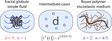
Figure 1: Illustration of the problem. The three panels represent different scenarios for a polymer whose folded configuration has a generic fractal dimension $d$, immersed in a viscoelastic medium characterized by a subdiffusive exponent $\alpha$. The middle panel illustrates the general case studied in this work. Left panel, limiting case of a space-filling fractal ($d=3$) in a simple Newtonian fluid. Right panel, limiting case of a Gaussian polymer in a viscoelastic medium. A scaling analysis predicts a subdiffusive exponent $2\alpha/(d+2)$ for the segment mean-square displacement $\langle r^{2}(t)\rangle$ in the Rouse regime. Hence, the two limiting cases of parameter values illustrated by the left and right panel cannot be distinguished by tracking single segments.

Moreover, the same scenario leads to specific predictions for the case of two-point correlations between different loci, at arc-length distance $s$ along the same chromosome Lampo et al. (2016), whereby more information can be extracted. As the lag time interval increases, the dynamics of loci pairs changes Lampo et al. (2016). This transition defines a characteristic time scale for the stress propagation between loci through the polymer backbone.

However, this scenario assumes an oversimplified picture of the folded state of the chromosome (which influences stress propagation). Indeed, chromosome packing typically does not follow the Rouse prediction for the static exponent Imakaev et al. (2015); Hofmann and Heermann (2015); Nicodemi and Pombo (2014) and, therefore (see, e.g., Tamm et al. (2015); Benza et al. (2012)), it is incompatible with the Rouse dynamics. Chromosome packing has been described in some cases by a fractal-globule model Grosberg et al. (1988, 1993); Lieberman-Aiden et al. (2009); Mirny (2011); Halverson et al. (2014) with fractal dimension $d=3$ instead of $d=2$ for a Rouse chain. More generally, the chromosome could effectively behave like a fractal (in a range of scales) with some fractal dimension due to the presence of a hierarchy of loops caused by bridging and/or loop-extruding protein complexes, which would affect both its local dynamics and the propagation of stresses. Figure 1 illustrates how the stress propagating through the embedding medium is felt by distant regions along the DNA chain in a fashion that it is dependent on the dimension of the folded state. Throughout this Letter we work under the simplifying assumption that the folded state is (in some range of length scales) self-similar; thus, its spatial organization can be described by a single static exponent.

In this Letter, we define a general scaling framework that takes into account both viscoelastic-like medium generating subdiffusion and arbitrary dimension of folded structure of a chromosome. We ask about the relative impact of these two ingredients on the stress-propagation time between loci pairs at given arclength distance on a chromosome. Additionally, based on a mathematical model for the Gaussian self-similar polymer states Amitai and Holcman (2013), we derive analytically the two-loci correlation functions, which depend on both medium and packing through their defining parameters. This calculation confirms our scaling argument and yields precise analytical estimates for the asymptotic behavior of the system. The results show how combining single-loci and two-loci tracking experiments might disentangle the contributions of medium viscoelasticity from the effects of the folded geometry of a chromosome.

Scaling considerations on the joint effects of fractal packing and viscoelasticity of the embedding medium.

We consider a polymer chain whose configuration is described by a function $R(n,t)$ where $n\in[0,N]$ is the (continuous or discrete) coordinate along the chain, and we assume that the chain conformation is fractal, i.e.,

$$\langle R^{2}(s,t)\rangle=\langle\left(R(n,t)-R(m,t)\right)^{2}\rangle=As^{2/d}\ ,$$ (1)

with some specific fractal dimension $d$. Here $s=|n-m|$ is the arclength distance. For long chains, and far from the chain ends, the prefactor $A$ in (1) becomes $m,n$-independent. The the long-time limit of the Rouse model corresponds to ideal polymer chains with $d=2$, while the compact fractal globule has $d=3$. For complex bacterial and eukaryotic chromosomes, the contributions of (i) incomplete relaxation to equilibrium Rosa and Everaers (2008), (ii) partial collapse Lieberman-Aiden et al. (2009); Odijk (1998), (iii) looped structures due to bridging proteins and active enzymes Nicodemi and Pombo (2014); Hofmann and Heermann (2015); Scolari and Cosentino Lagomarsino (2015); Imakaev et al. (2015); Dekker and Mirny (2016), and (iv) branched supercoiled structure due to plectonemes Benedetti et al. (2014) may result in a fractal-like organization (in a range of length scales) with $d$ between 2 and 3. The movement of a single locus on a chain can be characterized by the mean-square displacement

$$r^{2}(t)=\langle\left(R(n,t+t_{0})-R(n,t_{0})\right)^{2}\rangle_{t_{0}}\sim t^{2/z}\ ,$$ (2)

where $z$ is the so-called dynamic exponent and the averaging is over $t_{0}$. The standard argument Tamm et al. (2015) for a fractal structure in a simple fluid derives the connection between $z$ and fractal dimension $d$ by assuming that, due to stress propagation, at lag-time $t$, a region of spatial size $x(t)\sim t^{1/z}$ behaves as a single monomer. In the “free-draining” limit (negligible hydrodynamic interactions), the diffusion constant of this coherent region needs to depend on the number of monomers involved as $D_{\text{eff}}\sim\left(n(x(t))\right)^{-1}\sim x^{-d}$. Therefore, the mean-square diplacement of the region is $D_{\text{eff}}t\sim t^{1-d/z}$. Since the motion of the whole region and of a single monomer inside it have to follow the same behavior, one gets to the consistency condition $2/z=1-d/z$, i.e., $z=2+d$, the well-known result going back to De Gennes DeGennes (1976).

Importantly, this generalized Rouse approach relies on the assumption that chromosome chain dynamics is not restrained by topological entanglements, which is an open question in the current literature Rosa and Everaers (2008); Bruinsma et al. (2014). A proper description of the entanglement-dominated regime needs a generalization of the reptation model Doi and Edwards (1986) for polymer melts. Note that competing theories for such a reptation-like dynamics in fractal globules and ring melts have been suggested recently in the literature Smrek and Grosberg (2015); Ge et al. (2016).

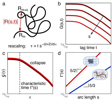
Figure 2: Scaling predictions for monomer-monomer correlations. A: Our calculations quantify stress propagation by the fluctuations of the physical distance between monomers at arclength distance $s$. B: Sketch of the decay (in log-log scale) of the correlation function $G(s,t)=\langle\left(R(n,t)-R(m,t)\right)\left(R(n,0)-R(m,0)\right)\rangle$, for different values of $s$. C: Our scaling analysis predicts the collapse of $G(s,t)$ on the master curve ${\cal G}$ upon rescaling of time by a characteristic scale $t^{*}(s)\sim s^{\frac{2+d}{\alpha d}}$. For each value of $s$, $t^{*}$ corresponds to a fixed value of $\tau$ in this plot. D: The characteristic time $t^{*}$ is a power law in $s$ (sketched here in log-log scale), which distinguishes the two limiting-case scenarios illustrated in Fig. 1.

Consider now a polymer whose monomers are embedded in a viscoelastic medium (cytoplasm or nucleoplasm), characterized by a scaling exponent $\alpha$, so that an isolated tracer particle moves subdiffusively with mean-square displacement $\langle x^{2}(t)\rangle$ growing with time as $D_{\alpha}t^{\alpha}$ with some $\alpha\leq 1$. The simplest assumption might be that the effects of polymer configuration and embedding medium on the monomer mean-square displacement are factorized, i.e., $R_{n}^{2}(t)\sim t^{2\alpha/z}$. Consider now simultaneous movement of two monomers separated by arclength distance $s$. At small times their displacements are essentially independent, but starting from some typical time, which we denote $t^{*}(s)$ their displacements become strongly coupled. This $t^{*}(s)$ gives an estimate of the time required for the stress to propagate between these two monomers. This time can be estimated as a time at which each monomer moves diffuses a distance comparable to the spatial distance between the two: $(t^{*})^{\alpha/z}\sim s^{1/d}$. Hence,

$$t^{*}\sim s^{z/(\alpha d)}=s^{(2+d)/(\alpha d)}.$$ (3)

The time scale $t^{*}(s)$ is expected to be measurable from two-point correlation functions, as described in ref. Lampo et al. (2016) for $d=2$.

These arguments, however, rely on an arbitrary assumption that the effects of medium and polymer folding can be factorized. The following scaling theory derives the same result based on more general dimensional grounds (Fig. 2). The monomer displacement and the monomer-to-monomer distance are expected to be scale invariant until the displacement becomes of order of the spatial size of the chain. Therefore, the one-locus mean-square displacement $r^{2}(t)$ and the two-point correlation function, defined as

$$\begin{array}[]{ll}G(s,t)=&\vskip 6.0pt plus 2.0pt minus 2.0pt\\ \langle\left(R(n,t+t_{0})-R(m,t+t_{0})\right)\left(R(n,t_{0})-R(m,t_{0})\right)\rangle_{t_{0}}&,\end{array}$$ (4)

are expected to obey the standard scaling forms

$$r^{2}(t)=Bt^{2/\zeta},\;\;G(s,t)=As^{2/d}{\cal G}(ts^{-b})$$ (5)

for the time lags $t\lesssim N^{\zeta/d}$. These conditions imply a scaling relation between $\zeta,d$ and $b$. Indeed, the scaling hypothesis implies invariance of all dimensionless quantities under the transformation $s\to\gamma s,\,t\to\gamma^{a}s$. Considering, in particular, $G(s,t)/r^{2}(t)$, this invariance implies $2a/z-2/d=a-b=0$, leading to $\zeta=bd$.

Hence, there is a single independent scaling exponent, which we can determine by a more rigorous version of the above argument Tamm et al. (2015). Assume that the physical properties of the medium are described by a subdiffusive fractional Langevin equation Lampo et al. (2016); Weber et al. (2010b), so that monomers obey the equation

$$\int_{0}^{t}dt^{\prime}K_{\alpha}(t-t^{\prime})\frac{dR_{i}(t^{\prime})}{dt^{\prime}}=f_{i}(t)+F_{i}^{\text{polym}}(t),$$ (6)

where $f_{i}$ is a random thermal force acting on the $i$-th monomer, $F_{i}^{\text{polym}}$ is a force acting on the $i$-th monomer from the other monomrers of the surrounding chain, and the memory kernel $K_{\alpha}$ is

$$K_{\alpha}(t)=D_{\alpha}\frac{(2-\alpha)(1-\alpha)}{|t|^{\alpha}},$$ (7)

which reduces to the standard Brownian kernel $K_{1}(t)=\delta(t)$ for $\alpha=1$. The fluctuation-dissipation theorem implies that the thermal noise $f(t)$ in the right-hand side of (6) satisfies $\langle f_{i}(t)f_{i}(t^{\prime})\rangle=K(t-t^{\prime})$.

Following Lampo et al. (2016) (and in the spirit of the original Rouse model), we also assume that the thermal forces acting on different monomers are uncorrelated, $\langle f_{i}(t)f_{j}(t^{\prime})\rangle=\delta_{i,j}K(t-t^{\prime})$. In this case, the effective diffusion constant for a group of monomers is inversely proportional to their number, as assumed above. Indeed, the equation of motion for the center of mass $R_{\text{c.m.}}(n,t)=n^{-1}\sum_{i=1}^{n}R(i,t)$ of a group of $n$ consequential monomers will include a random force of the form $f_{n}(t)=n^{-1}\sum_{i=1}^{n}f_{i}(t)$ whose correlator reads

$$\langle f_{n}(t,s)f_{n}(t^{\prime})\rangle=\frac{K(t-t^{\prime})}{n}=\frac{D_{\alpha}^{\text{eff}}(2-\alpha)(1-\alpha)}{|t-t^{\prime}|^{\alpha}}.$$ (8)

This implies for the monomer displacement

$$r^{2}(t)\sim t^{2/\zeta}\sim D_{\alpha}^{\text{eff}}t^{\alpha}\sim D_{\alpha}t^{\alpha}t^{-d/\zeta},$$ (9)

thus yielding

$$\zeta=\frac{2+d}{\alpha};\;b=\frac{2+d}{\alpha d}.$$ (10)

Eq. (10) is a direct generalization of the results of ref. Lampo et al. (2016) for the case of a fractally packed polymer and of ref. Tamm et al. (2015) for general viscoelastic embedding medium.

Analytical estimates of the correlation function for the beta model in a viscoelastic medium.

To give more solid grounds to the scaling considerations, we also defined an explicit model for a specific fractal packing of a polymer, generalizing the so-called “beta model” Amitai and Holcman (2013). This is a Gaussian generalization of the Rouse model that has the advantage of being mathematically tractable, and we extended it to the case of viscoelastic embedding medium Weber et al. (2010b).

The simplest way to define this model is in terms of the behavior of the Rouse modes $u_{p}(t),\,p=0...N-1$

$$u_{p}(t)=\sqrt{\frac{1+\delta_{0,p}}{N}}\int_{0}^{N}dsR(t,s)\cos\frac{p\pi(s-1/2)}{N}\ .$$ (11)

In the conventional Rouse model, these modes satisfy a set of independent Ornstein-Uhlenbeck equations

$$\frac{du_{p}}{dt}=-\kappa_{p}u_{p}+{f}_{p};\quad\kappa_{p}=\tau_{N}^{-1}\sin^{2}\left(\frac{\pi}{2}\frac{p}{N}\right)\ ,$$ (12)

where $\tau_{N}=a^{2}/4Dk_{b}T$ is a relaxation time scale (of order of the time needed for a monomer to diffuse by a distance equal to its own size $a$).

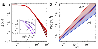
Figure 3: Analytical predictions from the beta model in viscoelastic medium correspond to the scaling expectations. A: Collapse of the two-point correlation function ${\cal G}(\tau,\epsilon)$, given by Eq. (17) as a function of $\tau$. The red curves refer to $d=3$, $\alpha=0.9$ and different values of $s$. Inset: change of slope of the master curve ${\cal G}$ with varying values of the polymer fractal dimension $d$ ($d=4/3,\ 2,\ 3\$, increasing with direction of arrow) at fixed $\alpha=0.9$. The dashed lines are the predictions of Eq. (21). B: Scaling of $t^{*}(s)$ (plotted in units of $C_{\alpha}^{-1}$) for $d=2$ (red) and $d=3$ (blue). The shaded areas of the two colors correspond to the empirically relevant interval, $0.8<\alpha<1$.

The beta model is formally defined by replacing the second power of the sine in $\sin^{2}\left(\frac{\pi}{2}\frac{p}{N}\right)$ with an arbitrary power $\beta$. The parameter $\beta$ then plays a role in the effective description of a fractal folding. In terms of the original Rouse equation, this corresponds to replacing the second derivative over the genomic coordinate by a fractional derivative of order $\beta$ (see Supplementary materials). Introducing a viscoelastic-like medium in this model corresponds to replacing in Eq. (31) the time derivative of order one with a fractional derivative as prescribed by Eq. (6). As a result, the Rouse modes now satisfy

$$\int_{0}^{t}dt^{\prime}K_{\alpha}(t-t^{\prime})\frac{du_{p}(t^{\prime})}{dt}=-\tau_{N}^{-1}\sin^{\beta}\left(\frac{\pi}{2}\frac{p}{N}\right)u_{p}(t)+f_{p}(t)$$ (13)

where the memory kernel $K_{\alpha}(t)$ is defined by Eq. (7), and the random force correlation function is $\langle f_{p}(t)f_{p^{\prime}}(t^{\prime})\rangle=K(t-t^{\prime})\delta_{p,p^{\prime}}$.

The connection between the model described by Eq. (13) and the scaling considerations above is established by the fact that regardless of the value of the viscoelastic exponent $\alpha$, the beta-model converges at long times to an equilibrium state in which mean-squared monomer-to-monomer distance satisfies

$$\langle(R_{n}(t)-R_{m}(t))^{2}\rangle\sim s^{\beta-1},$$ (14)

meaning that this equilibrium conformation is fractal, with fractal dimension $d$

$$d=\frac{2}{\beta-1}.$$ (15)

Additionally, single-monomer displacement scales as

$$\langle r^{2}(t)\rangle\sim t^{\alpha(\beta-1)/\beta},$$ (16)

yielding $\zeta=\frac{2\beta}{\alpha(\beta-1)}=\frac{2+d}{\alpha}$ which confirms Eq. (10).

Finally, and most importantly, the solution of Eq. (13) allows to compute directly the asymptotics of the scaling function ${\cal G}(\tau)$ defined in Eq. (5) for $N\to\infty$. Additionally, this calculation can be carried out accounting for finite-chain-size corrections to the long-chain limit. Indeed (see Supplementary materials), a more general scaling function ${\cal G}(\tau,\epsilon)$, where $\epsilon=s/N\ll 1$, can be estimated as

$${\cal G}(\tau,\epsilon)\sim\sum_{k=1}^{\infty}(-1)^{k+1}\frac{\pi^{2k}}{(2k)!}\int_{\epsilon}^{1}x^{2k-\beta}E_{\alpha}\left(-\tau^{\alpha}x^{\beta}\right)dx,$$ (17)

where $\tau=C_{\alpha}ts^{-b}=C_{\alpha}ts^{-\beta/\alpha}$, $C_{\alpha}=\left(\tau_{N}\Gamma(3-\alpha)\xi\right)^{-1/\alpha}$ is an $\alpha$-dependent constant with the dimension of an inverse time, and $E_{\alpha}(x)$ is the Mittag-Leffler function

$$E_{\alpha}(x)=\sum_{j=0}^{\infty}\frac{x^{j}}{\Gamma(1+\alpha j)},$$ (18)

which reduces to a simple exponential for $\alpha=1$. Importantly, the expression in Eq. (17) goes beyond the approximation of Eq. (5), as it allows for a small but finite value of $\epsilon$, while the scaling theory describes only the case of infinitely long chains ($\epsilon=0$).

Moreover, it is possible to express the integrals in Eq. (17) in terms of the 2,2-order Wright function

$${}_{2}\psi_{2}\left[z\bigg{|}\begin{matrix}(a_{1},\alpha_{1})&(a_{2},\alpha_{2})\\ (b_{1},\beta_{1})&(b_{2},\beta_{2})\end{matrix}\right]=\sum_{k=0}^{\infty}\frac{\Gamma(a_{1}+\alpha_{1}k)\Gamma(a_{2}+\alpha_{2}k)}{\Gamma(b_{1}+\beta_{1}k)\Gamma(b_{2}+\beta_{2}k)}\frac{z^{k}}{k!}\ ,$$ (19)

whose asymptotics are known Paris (2010); this allows to distinguish the three following regimes (see Supplementary materials for technical details):

In the short-time limit $\tau\ll 1$ one gets

$${\cal G}(\tau,\epsilon)={\cal G}(0,0)\left(1-A\exp\left(-C\tau^{\alpha}\right)\right)$$ (20)

At intermediate times, $\epsilon^{-\beta/\alpha}\gg\tau\gg 1$(this time-scale is much smaller than relaxation time of the whole chain and the scaling function in this regime remains $\epsilon$-independent) for the physically interesting case of $3/2\leq\beta<3$ (i.e., $1<d\leq 4$) the correlations decay as a power-law

$${\cal G}(\tau,\epsilon)\sim\tau^{\alpha(1-3\beta^{-1})}$$ (21)

These two $\epsilon$-independent regimes, visible in Fig.2, are in full agreement with the scaling theory. Indeed, Eqs. (20),(21) are of the type prescribed by Eqs.(5) and (10), and the crossover at $\tau^{*}=t^{*}s^{-\beta/\alpha}\approx 1$ leads to the estimate $t^{*}\sim s^{-\beta/\alpha}=s^{-(d+2)/d\alpha}$ coinsiding with (3).

Finally, for small but finite $\epsilon$ a third regime arises for $\tau\gg\epsilon^{-\beta/\alpha}$. It corresponds to the relaxation of the whole chain, and is akin to the behavior of single particle correlation functions in simple (for $\alpha=1$) and viscoelastic (for $\alpha<1$) medium:

$$\begin{array}[]{rlll}{\cal G}(\tau,\epsilon)&\sim&\epsilon^{1-2\beta}\exp\left(-C\tau\epsilon^{\beta}\right)&\text{ for }\alpha=1\vskip 6.0pt plus 2.0pt minus 2.0pt\\ {\cal G}(\tau,\epsilon)&\sim&\epsilon^{1-2\beta}\tau^{-\alpha}&\text{ for }\alpha<1\end{array}$$ (22)

In conclusion, the framework combining the beta model with the approach of Spakowitz and coworkers Weber et al. (2010b); Lampo et al. (2016) provides a valuable building block for the description of the motion of both eukaryotes chromatin and bacterial chromosomes Zidovska et al. (2013); Bruinsma et al. (2014); Kleckner et al. (2014); Pederson et al. (2015), which can be generalized to the case of nonequilibrium fluctuations Vandebroek and Vanderzande (2015).

The general picture defined here depicts a wider scenario for the stress propagation than the one recently proposed by Lampo et al. Lampo et al. (2016). The most important prediction is that a joint measurement of two functions $r^{2}(t)$ and $G(s,t)$ allows to disentangle the effects of chain organization and embedding medium. Indeed, two independent measurements of the exponents $z$ (from single-loci MSD) and $b$ (from two-loci correlations) allows to reconstruct $\alpha$ and $d$ as follows

$$d=\frac{1}{zb};\;\;\alpha=\frac{2zb+1}{b}\ .$$ (23)

Finally, we note that the results obtained here, as well as those of ref. Lampo et al. (2016), are concerned with a polymer embedded in a complex medium whose reaction is non-local in time but local in space, i.e. forces acting on different monomer units are assumed to be uncorrelated. It seems natural to expect that this locality in space may in fact break down in some viscoelastic media, and generalization of the results obtained above for such a spatially non-local case is an important and challenging task.

Supplementary materials

.1 Rouse model

The standard Rouse model takes into account only interactions with the neighbours along the polymer chain and does not consider any excluded volume effects Doi and Edwards (1986); Grosberg and Khokhlov (1994); Rubinstein and Colby (2003). In particular, it ignores any hydrodynamic interations between monomers. In the Rouse description the interaction of polymer chain with the solvent is strictly local, which is expressed mathematically by the fact that the random noise representing the thermal force acting on monomers is delta-correlated in space and time.

Under these simplifying assumptions, the Langevin equation of the system reads

$$\xi\frac{dR_{n}}{dt}=-\frac{\partial}{\partial R_{n}}\phi(R_{1},...,R_{N})+F_{n}$$ (24)

where $\xi$ is a friction coefficient, the potential energy of monomer-monomer interactions $\phi(R_{1},...,R_{N})$ is

$$\phi(R_{1},...,R_{N})=\frac{k}{2}\sum_{i=1}^{N-1}(R_{i}-R_{i+1})^{2};\quad k=\frac{Dk_{B}T}{a^{2}}$$ (25)

and the random thermal force $F_{n}$ satisfies

$$\langle F_{n}(t)F_{m}(t^{\prime})\rangle=2Dk_{B}T\xi\delta(t-t^{\prime})\delta_{n,m}$$ (26)

here $D$ is the space dimension.

Substituting (25) into (24) one gets Langevin equation in the form

$$\xi\frac{dR_{n}}{dt}=k(R_{n+1}+R_{n-1}-2R_{n})+F_{n},$$ (27)

which corresponds in the continuous limit to the Edwards-Wilkinson equation of the form

$$\xi\frac{\partial R(n,t)}{\partial t}=k\frac{\partial^{2}R(n,t)}{\partial n^{2}}+F(n,t)$$ (28)

Equation (39) can be diagnoalized by Fourier transform $\{R_{n}\}_{1}^{N}\to\{u_{p}\}_{0}^{N-1}$:

$$\alpha_{p}^{(n)}=\begin{cases}\sqrt{\frac{2}{N}}\cos\frac{p\pi(n-1/2)}{N},p=1,2,..,N-1\\ \sqrt{\frac{1}{N}},p=0\end{cases}$$ (29)

$$R_{n}(t)=\sum_{p=0}^{N-1}u_{p}(t)\alpha_{p}^{(n)};\quad u_{p}(t)=\sum_{n=1}^{N}R_{n}(t)\alpha_{p}^{(n)}$$ (30)

In these new coordinates the Langevin equations decouple, and the resulting equations are of Ornstein-Uhlenbeck type:

$$\xi\frac{du_{p}}{dt}=-\kappa_{p}u_{p}+{f}_{p};\quad\kappa_{p}=4k\sin^{2}\frac{p\pi}{2N}=\frac{4Dk_{B}T}{a^{2}}\sin^{2}\left(\frac{\pi}{2}\frac{p}{N}\right)$$ (31)

the corresponding relaxation time $t_{p}$ of a $p$-th Rouse modes is

$$t_{p}=\frac{\xi}{\kappa_{p}};\;\;t_{1}=t_{R}=N^{2}\frac{\xi a^{2}}{\pi^{2}Dk_{B}T}=N^{2}t_{N}$$ (32)

where the longest relaxation time $t_{1}$ is also often called the Rouse time of the chain $t_{R}$, and the microscopic timescale is defined by $t_{N}$ - a typical time it takes for a single monomer unit to diffuse at a distance equal to the typical distance between monomers $a$.

The random force in (31) is

$${f}_{p}(t)=\sum_{n=1}^{N}F_{n}(t)\alpha_{p}^{(n)};\;\;\langle{f}_{p}(t){f}_{q}(t^{\prime})\rangle=2Dk_{B}T\xi\delta(t-t^{\prime})\delta_{p,q}$$ (33)

The Rouse potential in normal coordinates adopts the form

$$\phi(u_{0},...,u_{N-1})=\frac{1}{2}\sum_{p=0}^{N-1}\kappa_{p}u_{p}^{2}$$ (34)

For $p=0$ (31) gives the equation on the center-of-mass displacement, which, since $\kappa_{0}=0$, reduces to the overdamped equation for Brownian motion with the friction coefficient $\xi_{0}=\xi N$ and initial condition $u_{0}(0)=0$.

For $p>0$ the formal solution of (31) reads

$$u_{p}(t)=u_{p}(0)\exp(-t/t_{p})+\xi^{-1}\int_{0}^{t}f_{p}(t^{\prime})\exp\left(-\frac{t-t^{\prime}}{t_{p}}\right)dt^{\prime},$$ (35)

at times much larger than $t_{p}$ the solution becomes independent of initial conditions and the mean-square displacement coverges to

$$\lim_{t\to\infty}\langle u_{p}^{2}(t)\rangle=\xi^{-2}\int_{-\infty}^{t}\int_{-\infty}^{t}\langle f_{p}(t^{\prime})f_{p}(t^{\prime\prime})\rangle\exp\left(-\frac{t-t^{\prime}}{t_{p}}\right)\exp\left(-\frac{t-t^{\prime\prime}}{t_{p}}\right)dt^{\prime}dt^{\prime\prime}=\frac{Dk_{B}T}{\kappa_{p}},$$ (36)

on the other hand, for $t\ll t_{p}$ the mean-square displacement of $u_{p}$ grows linearly with time as for normal diffusion:

$$\langle(u_{p}(t)-u_{p}(0))^{2}\rangle_{t\ll\tau_{p}}\sim\xi^{-2}\int_{0}^{t}\int_{0}^{t}\langle f_{p}(t^{\prime})f_{p}(t^{\prime\prime})\rangle dt^{\prime}dt^{\prime\prime}=\frac{2Dk_{B}T}{\xi}t$$ (37)

.2 Beta model

In the $t\gg t_{R}$ regime, the conformational statistics of a Rouse polymer chain converges to that of an ideal Gaussian polymer chain. In order to describe the dynamics of a chain with different equilibrium statistics (e.g., a swollen coil or a fractal globule) in the similar framework one needs to modify the Rouse equations in order to include the interactions between the monomers.

One possible way to do that is the so-called beta model introduced in ref. Amitai and Holcman (2013) which, despite having no clear microscopic justification, has the advantage of describing parametrically the fractal structure of the polymer conformations and at the same time being analytically tractable. The basic idea of the beta-model is to modify the structural potential $\phi(R_{1},...,R_{N})$ by introducing effective springs between monomers positioned arbitrarily far from each other along the chain. Monomer-monomer interactions in this model are relatively weak, but infinitely-ranged (contrary to typical molecular systems, where these interactions are strong but short-ranged). However, the beta model captures phenomenologically the main large-scale properties of a fractally organized polymer in the mean-field sense (this reasoning can be compared to arguments in support of using soft potentials in DPD simulations Groot and Warren (1997)).

If all the monomers are connected to each other by a set of springs, the generalized Rouse potential of the chain should read:

$$\tilde{\phi}(R_{1},...,R_{N})=\frac{1}{2}\sum_{i>j}a_{ij}(R_{i}-R_{j})^{2}=\frac{1}{2}\sum_{i=1}^{i=N}R_{i}^{2}\sum_{j\neq i}a_{ij}-\sum_{i>j}a_{ij}R_{i}R_{j},$$ (38)

the corresponding Langevin equation being

$$\xi\frac{dR_{n}}{dt}=\sum_{m\neq n}a_{mn}(R_{m}-R_{n})+F_{n},$$ (39)

Beta model Amitai and Holcman (2013) corresponds to a particular choice of $a_{ij}$ such that in the same normal coordinates $u_{p}$ (30) the generalized potential takes the form similar to (34):

$$\tilde{\phi}(u_{0},...,u_{N-1})=\frac{1}{2}\sum_{p=0}^{N-1}\tilde{\kappa}_{p}u_{p}^{2}$$ (40)

but with modified $\beta$-dependent eigenvalues

$$\tilde{\kappa}_{p}=\frac{4Dk_{B}T}{a^{2}}\sin^{\beta}\left(\frac{\pi}{2}\frac{p}{N}\right)$$ (41)

(thus $\beta=2$ corresponds to the regular Rouse model).

Using the inverse Fourier transform, one gets the following results for the original parameters $a_{ij}$ of the potential:

$$\tilde{\phi}(R_{1},...,R_{N})=\frac{1}{2}\sum_{p=0}^{N-1}\tilde{\kappa}_{p}\left(\sum_{n=1}^{N}R_{n}\alpha_{p}^{(n)}\right)^{2}=\frac{1}{2}\sum_{l,m=1}^{N}A_{lm}R_{l}R_{m},$$ (42)

where

$$A_{lm}=\sum_{p=0}^{N-1}\tilde{\kappa}_{p}\alpha_{p}^{(l)}\alpha_{p}^{(m)}=4k\frac{2}{N}\sum_{p=1}^{N-1}\sin^{\beta}\left(\frac{p\pi}{2N}\right)\cos\left(\left(l-\frac{1}{2}\right)\frac{p\pi}{N}\right)\cos\left(\left(m-\frac{1}{2}\right)\frac{p\pi}{N}\right)$$ (43)

Now comparing (38) and (42) one can notice that $A_{ll}=\sum_{j\neq l}a_{lj}$ and $A_{lm}=-2a_{lm}$ for $l\neq m$. If we insert $\beta=2$ into (43), it readily gives $A_{lm}=2(\delta_{l-m,0}-\delta_{|l-m|,1})$ getting us back to the Rouse model.

Similarly to the Rouse model, in the normal coordiantes the relaxation of the beta-model can be understood in terms of a set of simultaneously relaxing Ornstein-Uhlenbeck oscilators with relaxation time corresponding to the $p$-th mode being equal to $\xi\tilde{\kappa}_{p}^{-1}$. For long-range modes with $p\ll N$ the relaxation times can be approximated by $\frac{\xi a^{2}}{k_{B}T}\left(\frac{N}{p}\right)^{\beta}$, while in the traditional Rouse model the corresponding times are$\frac{\xi a^{2}}{k_{B}T}\left(\frac{N}{p}\right)^{2}$.

.3 Beta model in fractal environment and single monomer displacement

Consider now the behavior of the beta-model in a media where the monomers are subject to the generalized Langevin equation defined by equation (6) of the main text with $F_{\text{polym}}$ being the derivative of the beta-model potential, (42). Changing variables to the normal coordinates once again allows to decouple of the equations leading to:

$$\xi_{\alpha}\int_{0}^{t}dt^{\prime}K(t-t^{\prime})\frac{du_{p}(t^{\prime})}{dt}=-\tilde{\kappa}_{p}u_{p}(t)+\tilde{F}_{p}(t)$$ (44)

where eigenvalues $\tilde{\kappa}_{p}=4k\sin^{\beta}\left(\dfrac{p\pi}{2N}\right)$ and

$$\langle\tilde{F}_{p}(t)\tilde{F}_{q}(t^{\prime})\rangle=\xi_{\alpha}k_{B}TK(t-t^{\prime})\delta_{p,q}$$ (45)

The solution of this generalized Ornstein-Uhlenback problem can be obtained as follows. The correlation function of a $p$-th normal coordinate $C_{p}(t)=\langle u_{p}(t)u_{p}(0)\rangle$, satisfies:

$$\xi_{\alpha}\int_{0}^{t}dt^{\prime}K(t-t^{\prime})\frac{dC_{p}(t^{\prime})}{dt}=-\tilde{\kappa}_{p}C_{p}(t),$$ (46)

where we use the fact that the average noise is null, $\langle\tilde{F}_{p}(t)\rangle=0$. The solution of this equation is known to be Metzler and Klafter (2000)

$$C_{p}(t)=C_{p}(0)E_{\alpha}\left[-\left(\frac{t}{\tilde{t}_{p}}\right)^{\alpha}\right]$$ (47)

where $E_{\alpha}(x)$ is the Mittag-Leffler function Samko et al. (1993):

$$E_{\alpha}(x)=\sum_{j=0}^{\infty}\frac{x^{j}}{\Gamma(1+\alpha j)},$$ (48)

and

$$\tilde{t}_{p}=\left(\frac{\Gamma(3-\alpha)\xi}{\tilde{\kappa}_{p}}\right)^{1/\alpha}.$$ (49)

Note that the rightful dimensionality of time is achieved by a proper choice of dimensionality for generalized friction coefficient, $\xi_{\alpha}$, in the generalized Langevin equation.

At times much larger than $\tilde{t}_{p}$, the average values of the normal coordinates $\langle u_{p}(t)\rangle$ converge to zero, while their average squares $\langle u_{p}^{2}(t)\rangle$ converge to their equilibrium values, $Dk_{B}T\tilde{\kappa}_{p}^{-1}$, dictated by the equipartition theorem.

Consider now the monomer displacement $\langle r_{n}^{2}(t)\rangle$ for some given $n$ as a function of time which is a weighted sum of $C_{p}(t)$ with fixed coefficients of order 1. Assume also that we start observation at the equilibrated state so that average initial values of the normal coordinates are the same as their long-time limits:

$$\overline{u_{p}^{2}(0)}=\overline{C_{p}(0)}=\lim_{t\to\infty}\langle u_{p}^{2}(t)\rangle=Dk_{B}T\tilde{\kappa}_{p}^{-1},$$ (50)

where bar designates averaging over initial conditions, while angular brackets designate, as usual, averaging over the realization of the noise. Now, if the sum of $\overline{C_{p}(t)}$ is controlled by the terms with $1\ll p\ll N$ (i.e.. for times $\tilde{t}_{N}\ll t\ll\tilde{T}_{1}$ one can replace it with the integral

$$\langle r_{n}^{2}(t)\rangle=\sum_{p=1}^{N}2(\overline{C_{p}(0)}-\overline{C_{p}(t)})\left(\alpha_{p}^{(n)}\right)^{2}\sim\int_{1}^{N}(\overline{C_{p}(0)}-\overline{C_{p}(t)})dp=\int_{1}^{N}Dk_{B}T\tilde{\kappa}_{p}^{-1}\left(1-E_{\alpha}\left[-\left(\frac{t}{\tilde{t}_{p}}\right)^{\alpha}\right]\right)dp$$ (51)

and after changing variables to

$$x=\left(\frac{t}{\tilde{t}_{p}}\right)^{\alpha};\;\;\;\tilde{\kappa}_{p}=4k(\pi p/2N)^{\beta}=x\frac{\xi\Gamma(3-\alpha)}{t^{\alpha}};\;\;\;p=\frac{2N}{\pi}\left(\frac{x\xi\Gamma(3-\alpha)}{4k}\right)^{1/\beta}t^{\alpha/\beta}$$ (52)

one gets

$$\langle r_{n}^{2}(t)\rangle=\frac{k_{B}T}{\xi}N\left(\frac{\xi}{k}\right)^{1/\beta}t^{\alpha-\alpha/\beta}\times\text{(some dimensionless integral)}$$ (53)

Interestingly, this equation implies that the exponent governing the time dependence of $\langle r_{n}^{2}(t)\rangle$ is just a product of exponents for a free particle in viscoelastic fluid and the exponent for the beta-model in the standard Brownian regime (in particular, for $\beta=2$ one recoveres the result for the Rouse model in viscoelastic environment Lampo et al. (2016)).

.4 Monomer-monomer correlations in the beta model

Let us now consider the correlations of two monomer positions in the equilibrium state of the beta-model. The beta model (as well as the Rouse model) implies that the long-time limit solution converges to some distinct equilibrium state. For the Rouse model this state is known to be the ideal chain state (see Tamm et al. (2015)). We now discuss the equilibrium state associated to the beta model.

We analyze the autocorrelation function of monomer-to-monomer distance $R_{nm}(t)=R_{n}(t)-R_{m}(t)$:

$$\langle R_{nm}(t)R_{nm}(0)\rangle=\sum_{p=0}^{N-1}\langle u_{p}(t)u_{p}(0)\rangle(\alpha_{p}^{(n)}-\alpha_{p}^{(m)})^{2}$$ (54)

In the equilibritum state the products of Rouse coordinates are averaged over both the initial state and the realization of disorder, so combining (47),(48),(50) one gets

$$\langle u_{p}(t)u_{p}(0)\rangle=\overline{C_{p}(t)}=\overline{C_{p}(0)}E_{\alpha}\left[-\left(\frac{t}{\tilde{t}_{p}}\right)^{\alpha}\right]$$ (55)

Substituting the Fourier coefficients, one obtains:

$$\langle R_{nm}(t)R_{nm}(0)\rangle\sim a^{2}N^{-1}\sum_{p=1}^{N-1}\sin^{-\beta}\left(\frac{\pi p}{2N}\right)\sin^{2}\left(\frac{\pi p|n-m|}{2N}\right)\sin^{2}\left(\frac{\pi p(n+m)}{2N}\right)\overline{C_{p}(t)}$$ (56)

Except for the monomers very close to the end of the chain, i.e. $(n+m)\ll N$ or $(2N-n-m)\ll N$), the factor $\sin^{2}\left(\dfrac{\pi p(n+m)}{2N}\right)$ is a rapidly oscilating function of $p$ and, when replacing summation with integration we will simply approximate it by $1/2$. The main contribution into the remaining sum

$$\langle R_{nm}(t)R_{nm}(0)\rangle\sim a^{2}N^{-1}\sum_{p=1}^{N-1}\sin^{-\beta}\left(\frac{\pi p}{2N}\right)\sin^{2}\left(\frac{\pi p|n-m|}{2N}\right)\overline{C_{p}(t)}$$ (57)

comes from the first half-period of the second multiplier, $1\leq p\leq\frac{N}{|n-m|}$. Within this interval $\frac{p}{N}\leq\frac{1}{|n-m|}\ll 1$ and the first sine can be replaced by $\left(\pi p/2N\right)^{-\beta}$. Switching from summation to integration over variable $\lambda=p/N$ and expanding the second sine to the Taylor series, we have:

$$\langle R_{nm}(t)R_{nm}(0)\rangle=G(s,t)\sim\frac{a^{2}}{2}\left(\frac{2}{\pi}\right)^{\beta}\sum_{k=1}^{\infty}(-1)^{k+1}\frac{\pi^{2k}}{(2k)!}s^{2k}I_{\alpha}(k,s,t)$$ (58)

where, similarly to the main text we introduced $s=|n-m|$ and the notation $G(s,t)$ for the correlation function. The integral $I_{\alpha}(k,s,t)$ is defined as

$$I_{\alpha}(k,s,t)=\int_{N^{-1}}^{s^{-1}}\lambda^{2k-\beta}E_{\alpha}\left(-\lambda^{\beta}\left(\frac{t}{\tilde{t}_{N}}\right)^{\alpha}\right)d\lambda$$ (59)

for $\alpha<1$ (fractal medium), and

$$I_{1}(k,s,t)=\int_{N^{-1}}^{s^{-1}}\lambda^{2k-\beta}\exp(-t\lambda^{\beta}/\tilde{t}_{N})d\lambda$$ (60)

for $\alpha=1$ (Newtonian medium). Note, that since $k\geq 1$ these integrals (60)-(59) converge for all $\beta<3$.

In order to study the behavior of the correlation function at short times we expand the Mittag-Leffler function in (59) into Fourier seriesSamko et al. (1993). Changing the order of summation and integration, leads to the following series representation of the integrals in the limit $N\to\infty$:

$$I_{\alpha}(k,s,t)=s^{\beta-1-2k}\sum_{n=0}^{\infty}\frac{1}{\Gamma(\alpha n+1)(2k+\beta(n-1)+1)}\left(-\frac{t^{\alpha}}{\tilde{t}_{N}^{\alpha}s^{\beta}}\right)^{n}$$ (61)

Substituting this representation into autocorrelation function (58) leads to:

$$G(s,t)\sim a^{2}s^{\beta-1}\sum_{n=0}^{\infty}\frac{1}{\Gamma(\alpha n+1)}\left(-\frac{t^{\alpha}}{\tilde{t}_{N}^{\alpha}s^{\beta}}\right)^{n}\sum_{k=1}^{\infty}(-1)^{k+1}\frac{\pi^{2k}}{(2k)!}\frac{1}{2k+\beta(n-1)+1}$$ (62)

One sees therefore that at $t=0$

$$G(s,t=0)=\langle R_{nm}^{2}(0)\rangle\sim a^{2}s^{\beta-1}$$ (63)

independently of $\alpha$, i.e., the equilibrium state corresponding to the beta-model is fractal with fractal dimension $d=2/(\beta-1)$, confirming equation (15) of the main text.

Moreover, time dependence of the correlation function in the $N\to\infty$ limit is a function of a scaling dimensionless variable

$$\tau=\frac{t}{\tilde{t}_{N}s^{\beta/\alpha}}.$$ (64)

For $\tau\ll 1$ one expects the first terms of the series to be sufficient, and the resulting correlation function can be expressed in terms of a stretched exponent:

$$G(s,t)_{\tau\ll 1}\sim\frac{a^{2}s^{\beta-1}}{\Gamma(\alpha+1)}\left[\exp\left(-\tau^{\alpha}\right)+f(\beta)\Gamma(\alpha+1)-1\right]$$ (65)

where

$$f(\beta)=\sum_{k=1}^{\infty}(-1)^{k+1}\frac{\pi^{2k}}{(2k)!}\frac{1}{2k-\beta+1}$$ (66)

Now, for the behavior of (58) at longer times, $\tau\gtrsim 1$ the fact that $N$ is not infinite becomes important. It is instructive to introduce $\epsilon=s/N$ and rewrite the integral (59) in the form:

$$I_{\alpha}(k,s,\tau)=\frac{1}{\beta}\left(\frac{1}{\tau^{\alpha}s^{\beta}}\right)^{g(k)}\left[\gamma_{\alpha}\left(g(k),\tau^{\alpha}\right)-\gamma_{\alpha}\left(g(k),\epsilon^{\beta}\tau^{\alpha}\right)\right]$$ (67)

where $g(k)=(2k+1)\beta^{-1}-1$, and

$$\gamma_{\alpha}(a,z)=\int_{0}^{z}x^{a-1}E_{\alpha}(-x)dx$$ (68)

For $\alpha=1$ this function reduces to standard incomplete $\Gamma$-function (recall that $E_{1}(-x)=\exp(-x)$).

Consider the non-fractal case of $\alpha=1$ first. In this case it is known that for large $z$:

$$\gamma(a,z)\approx\Gamma(a)-z^{a-1}\exp(-z)$$ (69)

For $\epsilon^{-\alpha/\beta}\gg\tau\gg 1$ the integral in (60) is controlled by the upper bound resulting in:

$$I_{1}(k,s,\tau)\approx\frac{\Gamma(g(k))}{\beta}\left(\frac{1}{\tau s^{\beta}}\right)^{g(k)}-\frac{\exp\left(-\tau\right)}{\beta\tau}\frac{1}{s^{2k+1-\beta}}$$ (70)

In this intermediate regime, we may neglect the exponential term in (70) and leave only $k=1$ term in the $k$-series, which leads the following expression for $G(s,\tau)$

$$G(s,\tau)_{\frac{1}{\epsilon}\gg\tau\gg 1}\sim a^{2}\Gamma\left(\frac{3-\beta}{\beta}\right)s^{\beta-1}\tau^{-3\beta^{-1}+1}.$$ (71)

In turn, for $\tau\gg 1/\epsilon\gg 1$ $I_{1}$ is $s$-independent:

$$I_{1}(k,s,\tau)\approx\frac{1}{\beta\tau\epsilon^{\beta}}N^{-\beta g(k)}\exp\left(-\epsilon^{\beta}\tau\right)=\frac{\tau_{N}}{\beta tN^{\beta(g(k)-1)}}\exp\left(-\frac{t}{\tau_{N}N^{\beta}}\right)$$ (72)

resulting in the following long-time asymptotic of the autocorrelation function:

$$G(s,t)_{\tau\gg\epsilon^{-\beta}}\sim\frac{a^{2}\tau_{N}}{t}N^{2\beta-1}\exp\left(-\frac{t}{\tau_{N}N^{\beta}}\right)\left(1-\cos\frac{\pi s}{N}\right)$$ (73)

In order to proceed further in the case of $\alpha<1$, rewrite $\gamma_{\alpha}(a,z)$ in terms of the generalized Wright functionSamko et al. (1993):

$$\gamma_{\alpha}(a,z)={z^{s}}_{2}\psi_{2}\left[-z\bigg{|}\begin{matrix}(a,1)&(1,1)\\ (1,\alpha)&(1+a,1)\end{matrix}\right]$$ (74)

where, by definition:

$${}_{p}\psi_{q}\left[z\bigg{|}\begin{matrix}(a_{1},\alpha_{1})&(a_{2},\alpha_{2})&\cdots(a_{p},\alpha_{p})\\ (b_{1},\beta_{1})&(b_{2},\beta_{2})&\cdots(b_{q},\beta_{q})\end{matrix}\right]=\sum_{k=0}^{\infty}\frac{\prod_{r=1}^{p}\Gamma(a_{r}+\alpha_{r}k)}{\prod_{r=1}^{q}\Gamma(b_{r}+\beta_{r}k)}\frac{z^{k}}{k!}$$ (75)

Applying the known results for the asymptotics of the generalized Wright function Paris (2010), one obtains the following approximation for $I_{\alpha}(k,s,\tau)$ at intermediate times $\epsilon^{-\beta/\alpha}\gg\tau\gg 1$:

$$I_{\alpha}(k,s,\tau)\approx\dfrac{1}{\beta}s^{\beta-1-2k}\left[\tau^{-\alpha g}A_{1}(g)+\tau^{-\alpha}A_{2}(g)+2\tau^{-1}\exp\left(-\left|\cos\dfrac{\pi}{\alpha}\right|\tau\right)\cos\left(\dfrac{\pi}{\alpha}-\tau\sin\left(\dfrac{\pi}{\alpha}\right)\right)\right]$$ (76)

where

$$\begin{array}[]{rll}A_{1}(g)&=&\dfrac{\pi}{\sin\left(\pi g\right)}\dfrac{1}{\Gamma(1-\alpha g)}\vskip 6.0pt plus 2.0pt minus 2.0pt\\ A_{2}(g)&=&\dfrac{1}{(g-1)\Gamma(1-\alpha)}\end{array}$$ (77)

and we have omitted the $k$ dependence in $g(k)$ for brevity.

In the Newtonian case $\alpha=1$ the second prefactor $A_{2}(g)$ equals zero for all $k$, but for $\alpha<1$ both $A_{1}$ and $A_{2}$ are non-negligible and the comparative significance of respective terms in (76) depends on $\beta$. As a result, there are two different asymptotic regimes depending on $\beta$: for $3>\beta>3/2$ (which is the most physically interesting case) the leading term is $\tau^{-\alpha g(1)}$, while for $3/2>\beta>1$ the dominant term is simply $\tau^{-\alpha}$. Note that latter values of $\beta$ correspond to very dense polymer conformations with fractal dimension $d>4$, and it is not very surprising that corresponding globules move around essentially as point-like particles Deng and Barkai (2009).

As a result, at intermediate times and for $3>\beta>3/2$, the autocorrelation function reads:

$$G(s,\tau)_{\epsilon^{-\beta/\alpha}\gg\tau\gg 1}\sim a^{2}s^{\beta-1}\frac{\Gamma(x)\Gamma(1-x)}{\Gamma(1-\alpha x)}\left(\frac{1}{\tau}\right)^{\alpha w};\;\;w=g(1)=3\beta^{-1}-1.$$ (78)

In turn, for $3/2>\beta>1$:

$$G(s,\tau)_{\epsilon^{-\beta/\alpha}\gg\tau\gg 1}\sim a^{2}s^{\beta-1}\frac{f(2\beta)}{\Gamma(1-\alpha)}\frac{1}{\tau^{\alpha}}$$ (79)

Finally, in the large time limit, $\tau\gg\epsilon^{-\beta/\alpha}$ there is a single regime for all $0<\alpha<1$:

$$G(s,t)_{\tau\gg\epsilon^{-\beta/\alpha}}\sim\frac{a^{2}N^{2\beta-1}}{\Gamma(1-\alpha)t^{\alpha}}q(\beta,\epsilon)$$ (80)

where $q(\beta,x)$ is:

$$q(\beta,x)=\sum_{k=1}^{\infty}\frac{(-1)^{k+1}(\pi x)^{2k}}{(2k)!}\frac{x^{2\beta-2k-1}-1}{2k+1-2\beta}=x^{2\beta-1}f(2\beta)-\sum_{k=1}^{\infty}\frac{(-1)^{k+1}(\pi x)^{2k}}{(2k)!}\frac{1}{2k+1-2\beta}$$ (81)

In $\epsilon\ll 1$ limit one may leave only $k=1$ terms in the latter sum and asymptotic of $q(\beta,x)$ at $x\to 0$ depends again on values of $\beta$:

$$\begin{array}[]{rlll}q(\beta,x)_{x\ll 1}&\approx&\frac{x^{2}}{2\beta-3}&\mbox{ for }3/2<\beta<3\vskip 6.0pt plus 2.0pt minus 2.0pt\\ q(\beta,x)_{x\ll 1}&\approx&x^{2\beta-1}f(2\beta)&\mbox{ for }1<\beta<3/2\end{array}$$ (82)

References

- Dekker and Mirny (2016) J. Dekker and L. Mirny, Cell 164, 1110 (2016), ISSN 1097-4172.
- Benza et al. (2012) V. Benza, B. Bassetti, K. Dorfman, V. Scolari, K. Bromek, P. Cicuta, and M. Cosentino Lagomarsino, Rep. Prog. Phys. 75, 076602 (2012).
- Bronshtein et al. (2016) I. Bronshtein, I. Kanter, E. Kepten, M. Lindner, S. Berezin, Y. Shav-Tal, and Y. Garini, Nucleus 7, 27 (2016).
- Tiana et al. (2016) G. Tiana, A. Amitai, T. Pollex, T. Piolot, D. Holcman, E. Heard, and L. Giorgetti, Biophysical journal 110, 1234 (2016), ISSN 1542-0086.
- Amitai et al. (2015) A. Amitai, M. Toulouze, K. Dubrana, and D. Holcman, PLoS computational biology 11, e1004433 (2015), ISSN 1553-7358.
- Cosentino Lagomarsino et al. (2015) M. Cosentino Lagomarsino, O. Espéli, and I. Junier, FEBS Lett 589, 2996 (2015).
- Kleckner et al. (2014) N. Kleckner, J. K. Fisher, M. Stouf, M. A. White, D. Bates, and G. Witz, Curr Opin Microbiol 22, 127 (2014).
- Levi et al. (2005) V. Levi, Q. Ruan, M. Plutz, A. S. Belmont, and E. Gratton, Biophys. J. 89, 4275 (2005).
- Weber et al. (2010a) S. C. Weber, A. J. Spakowitz, and J. A. Theriot, Phys. Rev. Lett. 104, 238102 (2010a).
- Weber et al. (2012) S. C. Weber, A. J. Spakowitz, and J. A. Theriot, Proc. Natl. Acad. Sci. USA 109, 7338 (2012).
- Bronstein et al. (2009) I. Bronstein, Y. Israel, E. Kepten, S. Mai, Y. Shav-Tal, E. Barkai, and Y. Garini, Phys. Rev. Lett. 103, 018102 (2009).
- Javer et al. (2013) A. Javer, Z. Long, E. Nugent, M. Grisi, K. Siriwatwetchakul, K. D. Dorfman, P. Cicuta, and M. Cosentino Lagomarsino, Nat. Commun. 4, 3003 (2013).
- Javer et al. (2014) A. Javer, N. J. Kuwada, Z. Long, V. G. Benza, K. D. Dorfman, P. A. Wiggins, P. Cicuta, and M. C. Lagomarsino, Nat Commun 5, 3854 (2014).
- Rouse (1953) P. E. Rouse, The Journal of Chemical Physics 21, 1272 (1953).
- Doi and Edwards (1986) M. Doi and S. F. Edwards, The Theory of Polymer Dynamics (Oxford University Press, USA, 1986), ISBN 0198520336.
- Kepten et al. (2011) E. Kepten, I. Bronshtein, and Y. Garini, Phys Rev E Stat Nonlin Soft Matter Phys 83, 041919 (2011).
- Weber et al. (2010b) S. C. Weber, J. A. Theriot, and A. J. Spakowitz, Phys. Rev. E 82, 011913 (2010b).
- Lampo et al. (2016) T. J. Lampo, A. S. Kennard, and A. J. Spakowitz, Biophysical journal 110, 338 (2016), ISSN 1542-0086.
- Lampo et al. (2015) T. J. Lampo, N. J. Kuwada, P. A. Wiggins, and A. J. Spakowitz, Biophysical journal 108, 146 (2015), ISSN 1542-0086.
- Imakaev et al. (2015) M. V. Imakaev, G. Fudenberg, and L. A. Mirny, FEBS letters 589, 3031 (2015), ISSN 1873-3468.
- Hofmann and Heermann (2015) A. Hofmann and D. W. Heermann, FEBS letters 589, 2958 (2015), ISSN 1873-3468.
- Nicodemi and Pombo (2014) M. Nicodemi and A. Pombo, Current opinion in cell biology 28, 90 (2014), ISSN 1879-0410.
- Tamm et al. (2015) M. V. Tamm, L. I. Nazarov, A. A. Gavrilov, and A. V. Chertovich, Physical review letters 114, 178102 (2015), ISSN 1079-7114.
- Grosberg et al. (1988) A. Y. Grosberg, S. K. Nechaev, and E. I. Shakhnovich, Journal de physique 49, 2095 (1988).
- Grosberg et al. (1993) A. Y. Grosberg, Y. Rabin, S. Havlin, and A. Neer, Europhysics letters 23, 373 (1993).
- Lieberman-Aiden et al. (2009) E. Lieberman-Aiden, N. L. van Berkum, L. Williams, M. Imakaev, T. Ragoczy, A. Telling, I. Amit, B. R. Lajoie, P. J. Sabo, M. O. Dorschner, et al., Science 326, 289 (2009).
- Mirny (2011) L. A. Mirny, Chromosome Research 19, 37 (2011).
- Halverson et al. (2014) J. D. Halverson, J. Smrek, K. Kremer, and A. Y. Grosberg, Reports on Progress in Physics 77, 022601 (2014).
- Amitai and Holcman (2013) A. Amitai and D. Holcman, Physical review. E, Statistical, nonlinear, and soft matter physics 88, 052604 (2013), ISSN 1550-2376.
- Rosa and Everaers (2008) A. Rosa and R. Everaers, PLoS Comput Biol 4, e1000153 (2008).
- Odijk (1998) T. Odijk, Biophys. Chem. 73, 23 (1998).
- Scolari and Cosentino Lagomarsino (2015) V. F. Scolari and M. Cosentino Lagomarsino, Soft matter 11, 1677 (2015), ISSN 1744-6848.
- Benedetti et al. (2014) F. Benedetti, J. Dorier, Y. Burnier, and A. Stasiak, Nucleic acids research 42, 2848 (2014), ISSN 1362-4962.
- DeGennes (1976) P. DeGennes, Macromolecules 9, 587 (1976).
- Bruinsma et al. (2014) R. Bruinsma, A. Y. Grosberg, Y. Rabin, and A. Zidovska, Biophysical journal 106, 1871 (2014), ISSN 1542-0086.
- Smrek and Grosberg (2015) J. Smrek and A. Y. Grosberg, Journal of Physics: Condensed Matter 27, 064117 (2015).
- Ge et al. (2016) T. Ge, S. Panyukov, and M. Rubinstein, Macromolecules 49, 708 (2016).
- Paris (2010) R. B. Paris, European Journal of pure and applied mathematics 3, 1006 (2010).
- Zidovska et al. (2013) A. Zidovska, D. A. Weitz, and T. J. Mitchison, Proceedings of the National Academy of Sciences of the United States of America 110, 15555 (2013), ISSN 1091-6490.
- Pederson et al. (2015) T. Pederson, M. C. King, and J. F. Marko, Molecular biology of the cell 26, 3915 (2015), ISSN 1939-4586.
- Vandebroek and Vanderzande (2015) H. Vandebroek and C. Vanderzande, Physical Review E 92, 060601 (2015).
- Grosberg and Khokhlov (1994) A. Grosberg and A. Khokhlov, Statistical Physics of Macromolecules (AIP Press, Woodbury, NY, 1994).
- Rubinstein and Colby (2003) M. Rubinstein and R. Colby, Polymer Physics (Oxford University Press, Oxford, UK, 2003).
- Groot and Warren (1997) R. D. Groot and P. B. Warren, Journal of Chemical Physics 107, 4423 (1997).
- Metzler and Klafter (2000) R. Metzler and J. Klafter, Physics Reports 339, 1 (2000).
- Samko et al. (1993) S. G. Samko, A. A. Kilbas, and O. I. Marichev, Fractional integrals and derivatives. Theory and Applications (Gordon and Breach, Yverdon, 1993).
- Deng and Barkai (2009) W. Deng and E. Barkai, Phys. Rev. E 79, 011112 (2009).