Probabilistic properties of the elliptic motion

Abstract

In this paper we consider the plane elliptic motion which occurs if the moving centrode is a circle of radius $r$ and the fixed centrode a circle of radius $2r$. Every point of the moving plane generates an ellipse in the fixed plane. Let a disk of radius $R$, $0\leq R<\infty$, concentric to the moving centrode be attached to the moving plane. If a point $P$ is chosen at random from this disk, then the area and the perimeter of the ellipse generated by $P$ are random variables. We determine the moments and the distributions of these random variables for the case that $P$ is uniformly distributed over the area of the disk.
2010 Mathematics Subject Classification: 52A22, 53C65, 60D05, 53A17, 51N20, 33E05
Keywords: elliptic motion, random ellipses, area moments, area distribution, perimeter moments, perimeter distribution, centrode, elliptic integrals

1 Introduction

We consider a fixed Euclidean plane $S$ with a Cartesian frame of origin $O$ and $x,y$ axes, and a moving Euclidean plane $\varSigma$ with a Cartesian frame of origin $\varOmega$ and $\xi,\eta$ axes. To $\varSigma$ we attach a circle $C_{1}$ with centre $\varOmega$ and radius $r$; to $S$ we attach a circle $C_{0}$ with centre $O$ and radius $2r$ (see Fig. 2).

If $C_{1}$ rolls inside $C_{0}$, then every point $P$ fixed in $\varSigma$ generates an ellipse in $S$. Therefore, this motion is called elliptic motion. If $P=\varOmega$, then the ellipse is a circle with centre $O$ and radius $r$; if $P\in C_{1}$, then the ellipse degenerates to a (double) line segment of length $4r$ which is one diameter of $C_{0}$. [4, pp. 2-3, 8-9], [1, pp. 14-15]

We denote by $\varphi$ the angle between the $x$-axis and the line segment $\overline{\rule{0.0pt}{7.8245pt}{}O\varOmega}$. W.l.o.g. we assume that for $\varphi=0$ the $\xi$-axis lies on the $x$-axis and both axes have equal direction. Then the equation in complex form of the ellipse generated by $P$ is given by

$$X=X(\varphi)=r\,\mathrm{e}^{\mathrm{i}\varphi}+\varXi\,\mathrm{e}^{-\mathrm{i}\varphi}\,,\quad 0\leq\varphi<2\pi\,,$$ (1.1)

with

• $\varXi:=\varrho\,\mathrm{e}^{\mathrm{i}\alpha}$, where $\varrho$, $\alpha$ are the polar coordinates of $P$ with respect to the $\xi,\eta$-frame, or

• $\varXi:=\xi+\mathrm{i}\eta$, where $\xi$, $\eta$ are the Cartesian coordinates of $P$ with respect to the $\xi,\eta$-frame.

In the first case, from (1.1) we get

$$\left.\begin{array}[]{l@{\;=\;}c@{\;}c@{\;}l}x&r\cos\varphi&+&\varrho\cos(\varphi-\alpha)\,,\\[2.84544pt] y&r\sin\varphi&-&\varrho\sin(\varphi-\alpha)\end{array}\right\}$$ (1.2)

as parametric representation of the ellipse, and in the second case,

$$\left.\begin{array}[]{l@{\;=\;}c@{\;}c@{\;}c@{\;}c@{\;}l}x&r\cos\varphi&+&\xi\cos\varphi&+&\eta\sin\varphi\,,\\[2.84544pt] y&r\sin\varphi&+&\eta\cos\varphi&-&\xi\sin\varphi\,.\end{array}\right\}$$ (1.3)

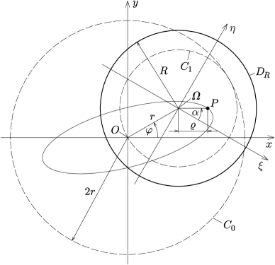
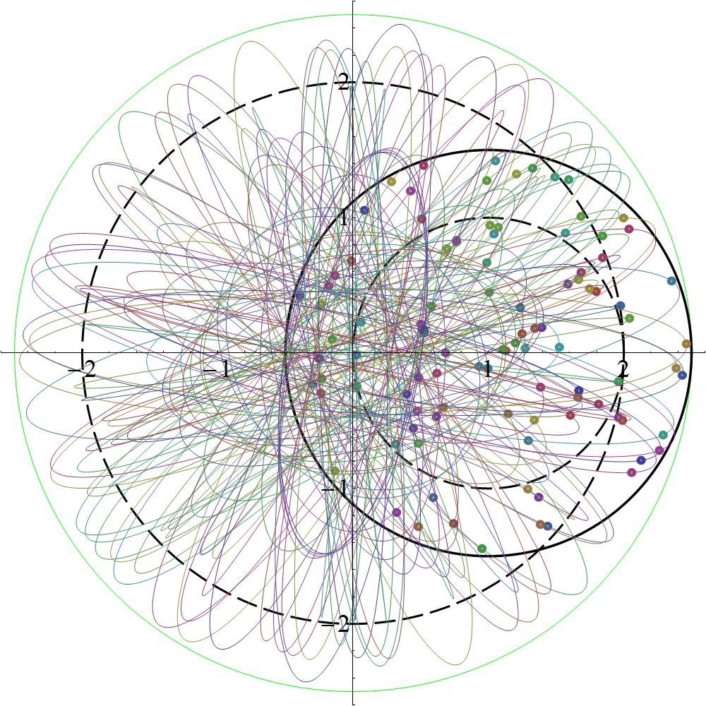
Fig.​ 1: Elliptic motion

Fig.​ 2: 100 random ellipses and their generating points; $r=1$, $R=1.5$

From (1.2) one finds that the length of the semi-major axis is equal to $r+\varrho$, and the length of the semi-minor axis equal to $|r-\varrho|$. Hence all points $P\in\varSigma$ with equal distance $\varrho$ from $\varOmega$ generate congruent ellipses. The centres of all ellipses lie in $O$. The angle between the $x$-axis and the major-axis of an ellipse is equal to $\alpha/2$.

$C_{0}$ is the fixed centrode and $C_{1}$ the moving centrode of the elliptic motion. It is possible to get the equations of $C_{0}$ and $C_{1}$ backwards from the equation(s) of the motion (1.1), (1.2) or (1.3). [4, p. 8-9], [1, p. 14-15] (For the notions of the fixed and the moving centrode see e. g [2, pp. 257-259].)

Now we consider a disk

$$D_{R}=\left\{(\xi,\eta)\in\varSigma\colon 0\leq\xi^{2}+\eta^{2}\leq R^{2}\right\},\quad 0\leq R<\infty\,.$$ (1.4)

If $P$ is chosen at random from $D_{R}$, then the area and the perimeter of the ellipse generated by $P$ are random variables which we denote by $A_{R}$ and $U_{R}$, respectively. In this paper we determine the moments and the distributions of these random variables for the case that $P$ is uniformly distributed over the area of $D_{R}$. Since $r$ is no essential parameter, we identify $A_{\varkappa}\equiv A_{R}$ and $U_{\varkappa}\equiv U_{R}$, where $\varkappa=R/r$

Fig. 2 shows the result of a simulation with 100 random points and ellipses.

2 Moments of the area

The moments of the random area $A_{R}$ enclosed by the ellipse generated by a random point $\in D_{R}$ (see (1.4)) are given by

$$\mathbb{E}\big{[}A_{R}^{k}\big{]}=\left(\int_{P\in D_{R}}A^{k}\,\mathrm{d}P\right)\bigg{/}\left(\int_{P\in D_{R}}\mathrm{d}P\right),$$

where $A$ is the area of the ellipse generated by the point $P\in D_{R}$, and $\mathrm{d}P=\mathrm{d}\xi\wedge\mathrm{d}\eta$ is the density for sets of points in the plane. Up to a constant factor this density is the only one that is invariant under motions [5, p. 13]. Due to the point symmetry we use the polar coordinates $\varrho,\alpha$. With $\xi=\varrho\cos\alpha$, $\eta=\varrho\sin\alpha$ we get

$$\mathrm{d}\xi={} \frac{\partial\xi}{\partial\varrho}\,\mathrm{d}\varrho+\frac{\partial\xi}{\partial\alpha}\,\mathrm{d}\alpha=\cos\alpha\,\mathrm{d}\varrho-\varrho\sin\alpha\,\mathrm{d}\alpha\,,$$

$$\mathrm{d}\eta={} \frac{\partial\eta}{\partial\varrho}\,\mathrm{d}\varrho+\frac{\partial\eta}{\partial\alpha}\,\mathrm{d}\alpha=\sin\alpha\,\mathrm{d}\varrho+\varrho\cos\alpha\,\mathrm{d}\alpha$$

and

$$\mathrm{d}\xi\wedge\mathrm{d}\eta={} \cos\alpha\sin\alpha\;\mathrm{d}\varrho\wedge\mathrm{d}\varrho+\varrho\cos^{2}\alpha\;\mathrm{d}\varrho\wedge\mathrm{d}\alpha-\varrho\sin^{2}\alpha\;\mathrm{d}\alpha\wedge\mathrm{d}\varrho-\varrho^{2}\sin\alpha\cos\alpha\;\mathrm{d}\alpha\wedge\mathrm{d}\alpha$$

$$={} \varrho\,\mathrm{d}\varrho\wedge\mathrm{d}\alpha\,,$$

hence

$$\mathbb{E}\big{[}A_{R}^{k}\big{]}=\frac{1}{\pi R^{2}}\int_{\alpha=0}^{2\pi}\,\int_{\varrho=0}^{R}A^{k}(\varrho)\,\varrho\,\mathrm{d}\varrho\,\mathrm{d}\alpha=\frac{2}{R^{2}}\int_{\varrho=0}^{R}A^{k}(\varrho)\,\varrho\,\mathrm{d}\varrho\,.$$ (2.1)

The area enclosed by an ellipse generated by a point $P\in D_{R}$ with distance $\varrho$ from $\varOmega$ is given by

$$A(\varrho)=\left\{\begin{array}[]{l@{\quad\mbox{if}\quad}l}\pi\left(r^{2}-\varrho^{2}\right)&0\leq\varrho\leq r\,,\\[2.84544pt] \pi\left(\varrho^{2}-r^{2}\right)&r<\varrho<\infty\,.\end{array}\right.$$ (2.2)

With $w=\varrho/r$, the area (2.2) function may be written as

$$\widetilde{A}(w)=\left\{\begin{array}[]{l@{\quad\mbox{if}\quad}l}\pi r^{2}\left(1-w^{2}\right)&0\leq w\leq 1\,,\\[2.84544pt] \pi r^{2}\left(w^{2}-1\right)&1<w<\infty\,.\end{array}\right.$$ (2.3)

Theorem 2.1.

The $k$-th moment, $k=1,2,\ldots$, of the random area $A_{\varkappa}\equiv A_{R}$, $\varkappa=R/r$, of an ellipse generated by a random point $P\in D_{R}$ ($P$ uniformly distributed over the area of the disk $D_{R}$) is given by

$$\mathbb{E}\big{[}A_{\varkappa}^{k}\big{]}=\left\{\begin{array}[]{l@{\quad\mbox{if}\quad}l}\pi^{k}r^{2k}&\varkappa=0\,,\\[5.69046pt] \dfrac{\pi^{k}r^{2k}}{k+1}\,\dfrac{1-(1-\varkappa^{2})^{k+1}}{\varkappa^{2}}&0<\varkappa\leq 1\,,\\[8.5359pt] \dfrac{\pi^{k}r^{2k}}{k+1}\,\dfrac{1+(\varkappa^{2}-1)^{k+1}}{\varkappa^{2}}&1<\varkappa<\infty\,.\end{array}\right.$$

Proof.

First, we consider the case $0<\varkappa\leq 1$ ($0<R\leq r$). Eq. (2.1) becomes

$$\mathbb{E}\big{[}A_{R}^{k}\big{]}=\frac{2\pi^{k}}{R^{2}}\int_{0}^{R}\left(r^{2}-\varrho^{2}\right)^{k}\varrho\>\mathrm{d}\varrho\,.$$

The substitution $\varrho=rw$ gives

$$\mathbb{E}\big{[}A_{R}^{k}\big{]}=\frac{2\pi^{k}r^{2k+2}}{R^{2}}\int_{w=0}^{R/r}\left(1-w^{2}\right)^{k}w\>\mathrm{d}w\,,$$

which, with $A_{\varkappa}\equiv A_{R}$ may also be written as

$$\mathbb{E}\big{[}A_{\varkappa}^{k}\big{]}=\frac{2\pi^{k}r^{2k}}{\varkappa^{2}}\int_{w=0}^{\varkappa}\left(1-w^{2}\right)^{k}w\>\mathrm{d}w\,.$$

The substitution

$$y=1-w^{2}\,,\quad\mathrm{d}y=-2w\,\mathrm{d}w\,,\quad\mathrm{d}w=-\frac{\mathrm{d}y}{2w}$$

yields

$$\mathbb{E}\big{[}A_{\varkappa}^{k}\big{]}={} -\frac{\pi^{k}r^{2k}}{\varkappa^{2}}\int_{y=1}^{1-\varkappa^{2}}y^{k}\>\mathrm{d}y=\frac{\pi^{k}r^{2k}}{\varkappa^{2}}\int_{1-\varkappa^{2}}^{1}y^{k}\>\mathrm{d}y=\frac{\pi^{k}r^{2k}}{\varkappa^{2}(k+1)}\>y^{k+1}\,\bigg{|}_{1-\varkappa^{2}}^{1}$$

$$={} \frac{\pi^{k}r^{2k}}{k+1}\>\frac{1-\left(1-\varkappa^{2}\right)^{k+1}}{\varkappa^{2}}\,.$$

Applying L’Hôpital’s rule we get

$$\lim_{\varkappa\rightarrow 0}\frac{1-\left(1-\varkappa^{2}\right)^{k+1}}{\varkappa^{2}}=\lim_{\varkappa\rightarrow 0}\frac{(k+1)\left(1-\varkappa^{2}\right)^{k}2\varkappa}{2\varkappa}=(k+1)\lim_{\varkappa\rightarrow 0}\left(1-\varkappa^{2}\right)^{k}=k+1\,,$$

hence

$$\mathbb{E}\big{[}A_{0}^{k}\big{]}=\pi^{k}r^{2k}\,.$$

Now we consider the case $1<\varkappa<\infty$ ($r<R<\infty$). Here we have

$$\mathbb{E}\big{[}A_{R}^{k}\big{]}={} \frac{2}{R^{2}}\int_{0}^{R}A^{k}(\varrho)\,\varrho\,\mathrm{d}\varrho=\frac{2}{R^{2}}\left(\int_{0}^{r}A^{k}(\varrho)\,\varrho\,\mathrm{d}\varrho+\int_{r}^{R}A^{k}(\varrho)\,\varrho\,\mathrm{d}\varrho\right)$$

$$={} \frac{2}{R^{2}}\left(\int_{0}^{r}\pi^{k}\left(r^{2}-\varrho^{2}\right)^{k}\varrho\>\mathrm{d}\varrho+\int_{r}^{R}\pi^{k}\left(\varrho^{2}-r^{2}\right)^{k}\varrho\>\mathrm{d}\varrho\right)$$

$$={} \frac{2\pi^{k}r^{2k+2}}{R^{2}}\left(\int_{0}^{1}\left(1-w^{2}\right)^{k}w\>\mathrm{d}w+\int_{1}^{R/r}\left(w^{2}-1\right)^{k}w\>\mathrm{d}w\right),$$

hence

$$\mathbb{E}\big{[}A_{\varkappa}^{k}\big{]}={} \frac{2\pi^{k}r^{2k}}{\varkappa^{2}}\left(\frac{1}{2(k+1)}+\int_{1}^{\varkappa}\left(w^{2}-1\right)^{k}w\>\mathrm{d}w\right)=\frac{2\pi^{k}r^{2k}}{\varkappa^{2}}\left(\frac{1}{2(k+1)}+\frac{\left(\varkappa^{2}-1\right)^{k+1}}{2(k+1)}\right)$$

$$={} \frac{\pi^{k}r^{2k}}{k+1}\,\frac{1+(\varkappa^{2}-1)^{k+1}}{\varkappa^{2}}\,.\qed$$

The graph of $\mathbb{E}[A_{\varkappa}]/r^{2}$ is shown in Fig. 4. For $\varkappa>1$ we have

$$\frac{\mathrm{d}}{\mathrm{d}\varkappa}\,\mathbb{E}[A_{\varkappa}]=\frac{\pi r^{2}\left(\varkappa^{4}-2\right)}{\varkappa^{3}}\,.$$

It follows that the expectation $\mathbb{E}[A_{\varkappa}]$ has its global minimum at point $\varkappa=\sqrt[4]{2}\approx 1.18921$ with value

$$\mathbb{E}\left[A_{\sqrt[4]{2}}\right]=\big{(}\sqrt{2}-1\big{)}\pi r^{2}\approx 1.30129\,r^{2}\,.$$

Furthermore one finds that

$$\mathbb{E}[A_{1}]=\mathbb{E}\left[A_{\sqrt{2}}\right]=\frac{1}{2}\,\pi r^{2}=\frac{1}{2}\,\widetilde{A}(0)=\frac{1}{2}\,\widetilde{A}\big{(}\sqrt{2}\,\big{)}=\frac{1}{2}\,\mathbb{E}[A_{0}]\,.$$

For the variance of $A_{\varkappa}$, $\mathbb{V}\mathrm{ar}[A_{\varkappa}]=\mathbb{E}[A_{\varkappa}^{2}]-\mathbb{E}[A_{\varkappa}]^{2}$, we get

$$\mathbb{V}\mathrm{ar}[A_{\varkappa}]=\frac{\pi^{2}r^{4}}{3}\,\frac{1-\left(1-\varkappa^{2}\right)^{3}}{\varkappa^{2}}-\frac{\pi^{2}r^{4}}{4}\,\frac{\left[1-\left(1-\varkappa^{2}\right)^{2}\right]^{2}}{\varkappa^{4}}=\frac{\pi^{2}r^{4}\varkappa^{4}}{12}$$

if $0\leq\varkappa\leq 1$, and

$$\mathbb{V}\mathrm{ar}[A_{\varkappa}]=\frac{\pi^{2}r^{4}}{3}\,\frac{1+\left(\varkappa^{2}-1\right)^{3}}{\varkappa^{2}}-\frac{\pi^{2}r^{4}}{4}\,\frac{\left[1+\left(\varkappa^{2}-1\right)^{2}\right]^{2}}{\varkappa^{4}}=\pi^{2}r^{4}\left[-1-\frac{1}{\varkappa^{4}}+\frac{2}{\varkappa^{2}}+\frac{\varkappa^{4}}{12}\right]$$

if $1<\varkappa<\infty$. One finds that $\mathbb{V}\mathrm{ar}[A_{\varkappa}]$ has local extrema at

$$\varkappa_{1}\approx 1.06840\quad\mbox{and}\quad\varkappa_{2}\approx 1.30621$$

with values

$$\mathbb{V}\mathrm{ar}[\varkappa_{1}]\approx 0.920036\quad\mbox{and}\quad\mathbb{V}\mathrm{ar}[\varkappa_{2}]\approx 0.703487\,,$$

respectively (see Fig. 4).

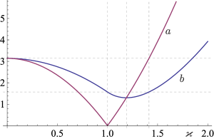
Fig.​ 3: a) $\widetilde{A}(\varkappa)/r^{2}$ (see (2.3)), b) $\mathbb{E}[A_{\varkappa}]/r^{2}$

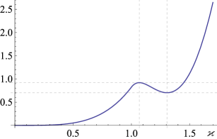
Fig.​ 4: $\mathbb{V}\mathrm{ar}[A_{\varkappa}]/r^{4}$

3 Distribution of the area

Now we determine the distribution function

$$F_{\varkappa}(x)=\mathbb{P}[A_{\varkappa}\leq x]$$

of the random variable $A_{\varkappa}$. We have to distinguish the following three cases.

• $0\leq R\leq r$ ($0\leq\varkappa\leq 1$): The smallest area of an ellipse is equal to $\pi(r^{2}-R^{2})$ and the biggest area equal to $\pi r^{2}$. We have $A_{R}>x$ if $P$ lies in an open disk with area $\pi\varrho^{2}$. From the first equation in (2.2), with $x=A$ we get

  $$\varrho^{2}=r^{2}\,\bigg{(}1-\frac{x}{\pi r^{2}}\bigg{)}\,.$$

  It follows that

  $$\mathbb{P}[A_{R}>x]=\frac{\pi\varrho^{2}}{\pi R^{2}}=\frac{r^{2}}{R^{2}}\,\bigg{(}1-\frac{x}{\pi r^{2}}\bigg{)}$$

  and

  $$\mathbb{P}[A_{R}\leq x]=1-\mathbb{P}[A_{R}>x]=1-\frac{r^{2}}{R^{2}}\,\bigg{(}1-\frac{x}{\pi r^{2}}\bigg{)}$$

  So we have

  $$F_{\varkappa}(x)=\left\{\begin{array}[]{l@{\quad\mbox{if}\quad}l}0&-\infty<x<\pi r^{2}\left(1-\varkappa^{2}\right),\\[2.84544pt] 1-\dfrac{1}{\varkappa^{2}}\,\bigg{(}1-\dfrac{x}{\pi r^{2}}\bigg{)}&\pi r^{2}\left(1-\varkappa^{2}\right)\leq x<\pi r^{2},\\[8.5359pt] 1&\pi r^{2}\leq x<\infty\,.\end{array}\right.$$

• $r\leq R\leq\sqrt{2}\,r$ ($1\leq\varkappa\leq\sqrt{2}$): For $0\leq A_{R}\leq\pi(R^{2}-r^{2})$ we have $A_{R}>x$ if $P$ lies

  • in an open disk with area $\pi\varrho^{2}$ or

  • in an open annulus with area $\pi(R^{2}-\varrho^{\prime 2})$, where $\varrho^{\prime}$ is the $\varrho$ in the second equation in (2.2).

  It follows that

  $$\mathbb{P}[A_{R}>x]={} \frac{\pi\varrho^{2}+\pi(R^{2}-\varrho^{\prime 2})}{\pi R^{2}}=1+\frac{\varrho^{2}-\varrho^{\prime 2}}{R^{2}}=1+\frac{r^{2}}{R^{2}}\,\bigg{[}1-\frac{x}{\pi r^{2}}-\bigg{(}1+\frac{x}{\pi r^{2}}\bigg{)}\bigg{]}$$

  $$={} 1-\frac{2x}{\pi R^{2}}\,,$$

  hence

  $$\mathbb{P}[A_{R}\leq x]=1-\mathbb{P}[A_{R}>x]=\frac{2x}{\pi R^{2}}\,.$$

  For $\pi(R^{2}-r^{2})\leq A_{R}\leq\pi r^{2}$ we have $A_{R}>x$ if $P$ lies in an open disk with area $\pi\varrho^{2}$. Therefore, the distribution function is given by

  $$F_{\varkappa}(x)=\left\{\begin{array}[]{l@{\quad\mbox{if}\quad}l}0&-\infty<x<0\,,\\[5.69046pt] \dfrac{2x}{\pi r^{2}\varkappa^{2}}&0\leq x<\pi r^{2}(\varkappa^{2}-1)\,,\\[8.5359pt] 1-\dfrac{1}{\varkappa^{2}}\,\bigg{(}1-\dfrac{x}{\pi r^{2}}\bigg{)}&\pi r^{2}\left(\varkappa^{2}-1\right)\leq x<\pi r^{2},\\[11.38092pt] 1&\pi r^{2}\leq x<\infty\,.\end{array}\right.$$

• $\sqrt{2}\,r\leq R<\infty$ ($\sqrt{2}\leq\varkappa<\infty$): One easily finds

  $$F_{\varkappa}(x)=\left\{\begin{array}[]{l@{\quad\mbox{if}\quad}l}0&-\infty<x<0\,,\\[5.69046pt] \dfrac{2x}{\pi r^{2}\varkappa^{2}}&0\leq x<\pi r^{2}\,,\\[8.5359pt] \dfrac{1}{\varkappa^{2}}\,\bigg{(}1+\dfrac{x}{\pi r^{2}}\bigg{)}&\pi r^{2}\leq x<\pi r^{2}\left(\varkappa^{2}-1\right),\\[11.38092pt] 1&\pi r^{2}\left(\varkappa^{2}-1\right)\leq x<\infty\,.\end{array}\right.$$

Now we determine the moments of the random variabe $A_{\varkappa}$ in an alternative way:

• $0\leq\varkappa\leq 1$: The density function is given by $f_{\varkappa}(x)=1/(\pi r^{2}\varkappa^{2})$ if $\pi r^{2}\left(1-\varkappa^{2}\right)\leq x<\pi r^{2}$, and $f_{\varkappa}(x)=0$ if the area is outside this interval. So we have

  $$\mathbb{E}\big{[}A_{\varkappa}^{k}\big{]}={} \int_{\pi r^{2}(1-\varkappa^{2})}^{\pi r^{2}}x^{k}f_{\varkappa}(x)\>\mathrm{d}x=\frac{1}{\pi r^{2}\varkappa^{2}}\int_{\pi r^{2}(1-\varkappa^{2})}^{\pi r^{2}}x^{k}\,\mathrm{d}x=\frac{\pi^{k}r^{2k}}{k+1}\,\frac{1-(1-\varkappa^{2})^{k+1}}{\varkappa^{2}}\,.$$

• $1\leq\varkappa\leq\sqrt{2}$ : The resctriction of the density function $f_{\varkappa}(x)$ to the interval $0\leq x\leq\pi r^{2}$ is given by

  $$f_{\varkappa}(x)=\frac{2}{\pi r^{2}\varkappa^{2}}\;\;\mbox{if}\;\;0\leq x<\pi r^{2}(\varkappa^{2}-1)\,,\quad\mbox{and}\quad f_{\varkappa}(x)=\frac{1}{\pi r^{2}\varkappa^{2}}\;\;\mbox{if}\;\;\pi r^{2}(\varkappa^{2}-1)\leq x\leq\pi r^{2}\,.$$

  It follows that

  $$\mathbb{E}\big{[}A_{\varkappa}^{k}\big{]}={} \frac{2}{\pi r^{2}\varkappa^{2}}\int_{0}^{\pi r^{2}(\varkappa^{2}-1)}x^{k}\,\mathrm{d}x+\frac{1}{\pi r^{2}\varkappa^{2}}\int_{\pi r^{2}(\varkappa^{2}-1)}^{\pi r^{2}}x^{k}\,\mathrm{d}x$$

  $$={} \frac{2\pi^{k}r^{2k}\left(\varkappa^{2}-1\right)^{k+1}}{(k+1)\varkappa^{2}}+\frac{\pi^{k}r^{2k}\left[1-\left(\varkappa^{2}-1\right)^{k+1}\right]}{(k+1)\varkappa^{2}}=\frac{\pi^{k}r^{2k}}{k+1}\,\frac{1+\left(\varkappa^{2}-1\right)^{k+1}}{\varkappa^{2}}\,.$$

• $\sqrt{2}\leq\varkappa<\infty$: One finds

  $$\mathbb{E}\big{[}A_{\varkappa}^{k}\big{]}={} \frac{2}{\pi r^{2}\varkappa^{2}}\int_{0}^{\pi r^{2}}x^{k}\,\mathrm{d}x+\frac{1}{\pi r^{2}\varkappa^{2}}\int_{\pi r^{2}}^{\pi r^{2}(\varkappa^{2}-1)}x^{k}\,\mathrm{d}x$$

  $$={} \frac{2\pi^{k}r^{2k}}{(k+1)\varkappa^{2}}+\frac{\pi^{k}r^{2k}\left[\left(\varkappa^{2}-1\right)^{k+1}-1\right]}{(k+1)\varkappa^{2}}=\frac{\pi^{k}r^{2k}}{k+1}\,\frac{1+\left(\varkappa^{2}-1\right)^{k+1}}{\varkappa^{2}}\,.$$

4 Moments of the perimeter

By analogy to the determination of $\mathbb{E}\big{[}A_{R}^{k}\big{]}$, we get the moments of the perimeter with

$$\mathbb{E}\big{[}U_{R}^{k}\big{]}={} \left(\int_{P\in D_{R}}u^{k}\,\mathrm{d}P\right)\bigg{/}\left(\int_{P\in D_{R}}\mathrm{d}P\right)=\frac{1}{\pi R^{2}}\int_{\alpha=0}^{2\pi}\,\int_{\varrho=0}^{R}u^{k}(\varrho)\,\varrho\,\mathrm{d}\varrho\,\mathrm{d}\alpha$$

$$={} \frac{2}{R^{2}}\int_{\varrho=0}^{R}u^{k}(\varrho)\,\varrho\,\mathrm{d}\varrho\,,$$

where $u(\varrho)$ is the perimeter of an ellipse generated by a point $P\in D_{R}$ with distance $\varrho$ from $\varOmega$. The length of the semi-major axis is given by $r+\varrho$, and the length of the semi-minor axis by $r-\varrho$ or $\varrho-r$. In both cases we have

$$u(\varrho)=4(r+\varrho)\>E\left(\frac{2\,\sqrt{\mathstrut r\varrho}}{r+\varrho}\right),$$ (4.1)

where

$$E(k)=\int_{0}^{\pi/2}\sqrt{1-k^{2}\sin^{2}\theta}\;\,\mathrm{d}\theta$$

is the complete elliptic integral of the second kind with modulus $k$, $0\leq k\leq 1$. So we have

$$\mathbb{E}\big{[}U_{R}^{k}\big{]}=\frac{2^{2k+1}}{R^{2}}\bigintsss_{\,0}^{R}\varrho\,(r+\varrho)^{k}\,E^{k}\!\left(\frac{2\,\sqrt{\mathstrut r\varrho}}{r+\varrho}\right)\mathrm{d}\varrho\,.$$ (4.2)

By substituting $w=\varrho/r$, the perimeter (4.1) may be written as

$$\tilde{u}(w)=rh(w)\,,\quad\mbox{where}\quad h(w):=4(w+1)\>E\left(\frac{2\,\sqrt{\mathstrut w}}{w+1}\right),$$ (4.3)

and, with $U_{\varkappa}\equiv U_{R}$, $\varkappa=R/r$, the integral (4.2) becomes

$$\mathbb{E}\big{[}U_{\varkappa}^{k}\big{]}=\frac{2^{2k+1}r^{k}}{\varkappa^{2}}\bigintsss_{\,0}^{\varkappa}w\,(w+1)^{k}\,E^{k}\!\left(\frac{2\,\sqrt{\mathstrut w}}{w+1}\right)\mathrm{d}w\,.$$ (4.4)

Theorem 4.1.

The expectation of the random perimeter $U_{\varkappa}=U_{R}$, $\varkappa=R/r$, of an ellipse generated by a random point $P\in D_{R}$ ($P$ uniformly distributed over the area of the disk $D_{R}$) is given by

$$\mathbb{E}[U_{\varkappa}]=\left\{\begin{array}[]{l@{\quad\mbox{if}\quad}l}2\pi r&\varkappa=0\,,\\[2.84544pt] \dfrac{8r}{9\varkappa^{2}}\left[\left(7\varkappa^{2}+1\right)E(\varkappa)+\left(3\varkappa^{4}-2\varkappa^{2}-1\right)K(\varkappa)\right]&0<\varkappa<1\,,\\[8.5359pt] 64r/9&\varkappa=1\,,\\[4.26773pt] \dfrac{8r}{9\varkappa}\left[\left(7\varkappa^{2}+1\right)E\!\left(\varkappa^{-1}\right)-4\left(\varkappa^{2}-1\right)K\!\left(\varkappa^{-1}\right)\right]&\varkappa>1\end{array}\right.$$

where

$$K(k)=\int\limits_{0}^{\pi/2}\frac{\mathrm{d}\theta}{\sqrt{1-k^{2}\sin^{2}\theta}}$$

is the complete elliptic integral of the first kind with modulus $k$, $0\leq k\leq 1$. The expectations for the cases $0<\varkappa<1$ and $\varkappa>1$ can be subsumed in the formula

$$\mathbb{E}[U_{\varkappa}]=\frac{4(\varkappa+1)r}{9\varkappa^{2}}\left[\left(7\varkappa^{2}+1\right)E\left(\frac{2\,\sqrt{\mathstrut\varkappa}}{\varkappa+1}\right)-(\varkappa-1)^{2}\,K\left(\frac{2\,\sqrt{\mathstrut\varkappa}}{\varkappa+1}\right)\right].$$

Proof.

First, we consider the case $0<\varkappa<1$. Using the relation

$$E\left(\frac{2\,\sqrt{k}}{1+k}\right)=\frac{1}{1+k}\left[2E(k)-\left(1-k^{2}\right)K(k)\right]$$ (4.5)

([3, Vol. 2, p. 299], Eq. (8.126.4)), (4.4) becomes

$$\mathbb{E}[U_{\varkappa}]=\frac{8r}{\varkappa^{2}}\left[2\int_{0}^{\varkappa}wE(w)\,\mathrm{d}w-\int_{0}^{\varkappa}wK(w)\,\mathrm{d}w+\int_{0}^{\varkappa}w^{3}K(w)\,\mathrm{d}w\right].$$

With

$$\int E(k)\,k\,\mathrm{d}k=\frac{1}{3}\left[\left(1+k^{2}\right)E(k)-(1-k^{2})K(k)\right],$$

$$\int K(k)\,k\,\mathrm{d}k=E(k)-(1-k^{2})K(k)\,,$$

$$\int K(k)\,k^{3}\,\mathrm{d}k=\frac{1}{9}\left[\left(4+k^{2}\right)E(k)-\left(1-k^{2}\right)\left(4+3k^{2}\right)K(k)\right]$$

(Equations (5.112.4), (5.112.3), (5.112.5) in [3, Vol. 2, p. 13]) we get

$$\mathbb{E}[U_{\varkappa}]=\frac{8r}{9\varkappa^{2}}\left[\left(7\varkappa^{2}+1\right)E(\varkappa)+\left(3\varkappa^{4}-2\varkappa^{2}-1\right)K(\varkappa)\right],\quad 0<\varkappa<1\,.$$ (4.6)

For $\varkappa=0$ we have $E(\varkappa)=\pi/2=K(\varkappa)$, hence

$$\left(7\varkappa^{2}+1\right)E(\varkappa)+\left(3\varkappa^{4}-2\varkappa^{2}-1\right)K(\varkappa)=0\,.$$

So $\mathbb{E}[U_{\varkappa}]$ has the indeterminate form $0/0$. Taking

$$\frac{\mathrm{d}E(k)}{\mathrm{d}k}=\frac{E(k)-K(k)}{k}\quad\mbox{and}\quad\frac{\mathrm{d}K(k)}{\mathrm{d}k}=\frac{E(k)-(1-k^{2})K(k)}{k(1-k^{2})}$$

(Equations (8.123.4), (8.123.2) in [3, Vol. 2, p. 298]) into account, applying L’Hôpital’s rule twice gives

$$\lim_{\varkappa\rightarrow 0}\mathbb{E}[U_{\varkappa}]=4r\lim_{\varkappa\rightarrow 0}\left[3E(\varkappa)+2\left(\varkappa^{2}-1\right)K(\varkappa)\right]=4r\left[3\,\frac{\pi}{2}-2\,\frac{\pi}{2}\right]=2\pi r\,.$$

Now we consider the limit of (4.6) for $\varkappa\rightarrow 1$ (and hence $R\rightarrow r$). We have $E(1)=1$, $K(1)=\infty$. For $\varkappa=1$,

$$\left(3\varkappa^{4}-2\varkappa^{2}-1\right)K(\varkappa)$$

has the indeterminate form $0\cdot\infty$. Mathematica finds

$$\lim_{\varkappa\rightarrow 1-}(3\varkappa^{4}-2\varkappa^{2}-1)K(\varkappa)=0\,.$$

It follows that

$$\lim_{\varkappa\rightarrow 1-}\mathbb{E}[U_{\varkappa}]=\frac{8r}{9\cdot 1}\left[(7+1)+0\right]=\frac{64r}{9}\,.$$

Now we consider the case $\varkappa=R/r>1$. Here we have

$$\mathbb{E}[U_{\varkappa}]={} \frac{64r}{9\varkappa^{2}}+\frac{8}{R^{2}}\bigintsss_{\,\varrho=r}^{R}\varrho\,(r+\varrho)\>E\left(\frac{2\,\sqrt{\mathstrut r\varrho}}{r+\varrho}\right)\mathrm{d}\varrho$$

$$={} \frac{64r}{9\varkappa^{2}}+\frac{8}{R^{2}}\bigintsss_{\,\varrho=r}^{R}\varrho^{2}\left(\frac{r}{\varrho}+1\right)\,E\left(\frac{2\,\sqrt{\mathstrut r/\varrho}}{(r/\varrho)+1}\right)\mathrm{d}\varrho\,.$$

The substitution

$$v=\frac{r}{\varrho}\,,\quad\mathrm{d}v=-\frac{r}{\varrho^{2}}\,\mathrm{d}\varrho\,,\quad\mathrm{d}\varrho=-\frac{r}{v^{2}}\,\mathrm{d}v\,,\quad\varrho=r\>\Longrightarrow\>v=1\,,\quad\varrho=R\>\Longrightarrow\>v=r/R=1/\varkappa$$

gives

$$\mathbb{E}[U_{\varkappa}]=\frac{64r}{9\varkappa^{2}}+\frac{8r}{\varkappa^{2}}\bigintsss_{\,1/\varkappa}^{1}\frac{v+1}{v^{4}}\>E\left(\frac{2\,\sqrt{v}}{1+v}\right)\mathrm{d}v\,.$$

Applying (4.5), we get

$$\mathbb{E}[U_{\varkappa}]=\frac{64r}{9\varkappa^{2}}+\frac{8r}{\varkappa^{2}}\left[2\int_{1/\varkappa}^{1}\frac{E(v)}{v^{4}}\>\mathrm{d}v-\int_{1/\varkappa}^{1}\frac{K(v)}{v^{4}}\>\mathrm{d}v+\int_{1/\varkappa}^{1}\frac{K(v)}{v^{2}}\>\mathrm{d}v\right]$$

From [3, Vol. 2, pp. 13-14], Equations (5.112.12), (5.112.9), we know that

$$\int\frac{E(k)}{k^{4}}\>\mathrm{d}k=\frac{1}{9k^{3}}\left[2\left(k^{2}-2\right)E(k)+\left(1-k^{2}\right)K(k)\right],$$

$$\int\frac{K(k)}{k^{2}}\>\mathrm{d}k=-\frac{E(k)}{k}\,.$$

Mathematica finds

$$\int_{1/\varkappa}^{1}\frac{K(v)}{v^{4}}\>\mathrm{d}v=\frac{1}{9}\left[-5+\varkappa\left(\varkappa^{2}+4\right)E\!\left(\varkappa^{-1}\right)+2\varkappa\left(\varkappa^{2}-1\right)K\!\left(\varkappa^{-1}\right)\right].$$

So we get

$$\mathbb{E}[U_{\varkappa}]=\frac{8r}{9\varkappa}\left[\left(7\varkappa^{2}+1\right)E\!\left(\varkappa^{-1}\right)-4\left(\varkappa^{2}-1\right)K\!\left(\varkappa^{-1}\right)\right],\quad\varkappa>1\,.$$

For $\varkappa=1$,

$$\left(\varkappa^{2}-1\right)K\!\left(\varkappa^{-1}\right)$$

has the indeterminate form $0\cdot\infty$. Mathematica finds

$$\lim_{\varkappa\rightarrow 1+}\left(\varkappa^{2}-1\right)K\!\left(\varkappa^{-1}\right)=0\,.$$

It follows that

$$\lim_{\varkappa\rightarrow 1+}\mathbb{E}[U_{\varkappa}]=\frac{8r}{9\cdot 1}\left[(7+1)-0\right]=\frac{64r}{9}\,.$$

Using the relations (4.5) and

$$K\left(\frac{2\,\sqrt{k}}{1+k}\right)=(1+k)K(k)$$

[3, Vol. 2, p. 299], Eq. (8.126.3), for $0<\varkappa<1$ we get

$$f(\varkappa):={} \frac{4(\varkappa+1)r}{9\varkappa^{2}}\left[\left(7\varkappa^{2}+1\right)E\left(\frac{2\,\sqrt{\mathstrut\varkappa}}{\varkappa+1}\right)-(\varkappa-1)^{2}\,K\left(\frac{2\,\sqrt{\mathstrut\varkappa}}{\varkappa+1}\right)\right]$$

$$={} \dfrac{8r}{9\varkappa^{2}}\left[\left(7\varkappa^{2}+1\right)E(\varkappa)+\left(3\varkappa^{4}-2\varkappa^{2}-1\right)K(\varkappa)\right]=\mathbb{E}[U_{\varkappa}]\,.$$

For $\varkappa>1$ we have

$$E\left(\frac{2\,\sqrt{\mathstrut\varkappa}}{\varkappa+1}\right)={} E\left(\frac{2\,\sqrt{\mathstrut\varkappa^{-1}}}{1+\varkappa^{-1}}\right)=\frac{1}{1+\varkappa^{-1}}\left[2E\!\left(\varkappa^{-1}\right)-\left(1-\varkappa^{-2}\right)K\!\left(\varkappa^{-1}\right)\right]$$

$$={} \frac{2\varkappa}{\varkappa+1}\,E\!\left(\varkappa^{-1}\right)-\frac{\varkappa-1}{\varkappa}\,K\!\left(\varkappa^{-1}\right)$$

and

$$K\left(\frac{2\,\sqrt{\mathstrut\varkappa}}{\varkappa+1}\right)=K\left(\frac{2\,\sqrt{\mathstrut\varkappa^{-1}}}{1+\varkappa^{-1}}\right)=\frac{\varkappa+1}{\varkappa}\,K\!\left(\varkappa^{-1}\right).$$

It follows that

$$f(\varkappa)={} \frac{4r}{9\varkappa^{2}}\left[2\varkappa\left(7\varkappa^{2}+1\right)E\!\left(\varkappa^{-1}\right)-8\varkappa\left(\varkappa^{2}-1\right)K\!\left(\varkappa^{-1}\right)\right]$$

$$={} \frac{8r}{9\varkappa}\left[\left(7\varkappa^{2}+1\right)E\!\left(\varkappa^{-1}\right)-4\left(\varkappa^{2}-1\right)K\!\left(\varkappa^{-1}\right)\right]=\mathbb{E}[U_{\varkappa}]\,.$$

For $\varkappa=0$,

$$\left(7\varkappa^{2}+1\right)E\left(\frac{2\,\sqrt{\mathstrut\varkappa}}{\varkappa+1}\right)-(\varkappa-1)^{2}\,K\left(\frac{2\,\sqrt{\mathstrut\varkappa}}{\varkappa+1}\right)=0\,,$$

hence $f(0)$ has the indeterminate form $0/0$. For $\varkappa=1$,

$$(\varkappa-1)^{2}\,K\left(\frac{2\,\sqrt{\mathstrut\varkappa}}{\varkappa+1}\right)$$

has the indeterminate form $0\cdot\infty$. Mathematica finds

$$\lim_{\varkappa\rightarrow 0}f(\varkappa)=2\pi r\qquad\mbox{and}\qquad\lim_{\varkappa\rightarrow 1}f(\varkappa)=\frac{64r}{9}\,.\qed$$

The graph of $\mathbb{E}[U_{\varkappa}]/r$ is shown in Fig. 5. Mathematica finds the series expansion

$$\mathbb{E}[U_{\varkappa}]=\pi r\left(\frac{4\varkappa}{3}+\frac{1}{\varkappa}-\frac{1}{16\varkappa^{3}}\right)+O\left(\varkappa^{-5}\right)$$

about the point $\varkappa=\infty$. For abbreviation we put

$$s(\varkappa):=\pi r\left(\frac{4\varkappa}{3}+\frac{1}{\varkappa}-\frac{1}{16\varkappa^{3}}\right).$$ (4.7)

$s(\varkappa)$ provides a very good approximation for $\mathbb{E}[U_{\varkappa}]$ even for relatively small values of $\varkappa$ (see Fig. 5). One finds that

$$\mathbb{E}[U_{1}]-s(1)\approx-2.29222\cdot 10^{-2}\,r\,,\qquad\mathbb{E}[U_{2}]-s(2)\approx-5.44238\cdot 10^{-4}\,r\,,$$

$$\mathbb{E}[U_{10}]-s(10)\approx-1.64009\cdot 10^{-7}\,r\,.$$

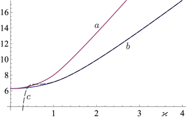
Fig.​ 5: a) $\tilde{u}(\varkappa)/r$ (see (4.3)),  b) $\mathbb{E}[U_{\varkappa}]/r$,  c) $s(\varkappa)/r$

5 Distribution of the perimeter

With (4.3) the maximum perimeter in the disk of radius $R$ is given by

$$\tilde{u}(\varkappa)=rh(\varkappa)\quad\mbox{with}\quad\varkappa=R/r\,.$$

Let $G_{\varkappa}(u)=\mathbb{P}[U_{\varkappa}\leq u]$ be the distribution function of the random variable $U_{\varkappa}$. One easliy finds from geometrical considerations

$$G_{\varkappa}(u)=\left\{\begin{array}[]{l@{\quad\mbox{if}\quad}l}0&-\infty<u<2\pi r\,,\\[1.42271pt] \dfrac{w^{2}(u)}{\varkappa^{2}}&2\pi r\leq u<rh(\varkappa)\,,\\[8.5359pt] 1&rh(\varkappa)\leq u<\infty\,,\end{array}\right.$$ (5.1)

where $w=w(u)$ is the solution of

$$rh(w)=u\,.$$

The Figures 7-11 show examples for graphs of distribution functions $G_{\varkappa}$ and corresponding density functions $g_{\varkappa}$ (multiplied with $r$). The density functions are obtained by numerical differentiation of the distribution functions. For comparison the distribution function and the density function (multiplied with $r$) of the uniform distribution with support interval $2\pi r\leq u\leq rh(\varkappa)$ are shown (dashed lines).

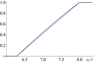
Fig.​ 6: Distribution function $G_{1}(u)$

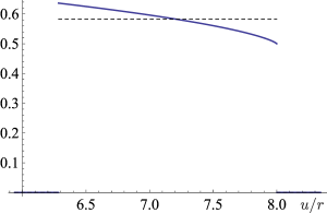
Fig.​ 7: Density function $rg_{1}(u)$

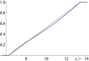
Fig.​ 8: Distribution function $G_{2}(u)$

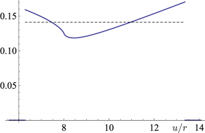
Fig.​ 9: Density function $rg_{2}(u)$

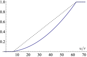
Fig.​ 10: Distribution function $G_{10}(u)$

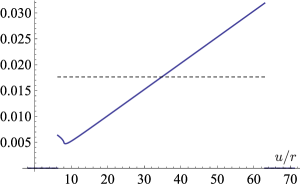
Fig.​ 11: Density function $rg_{10}(u)$

For the $k$-th moment of the perimeter $U_{\varkappa}$ we have the Stieltjes integral

$$\mathbb{E}\big{[}U_{\varkappa}^{k}\big{]}=\int_{-\infty}^{\infty}u^{k}\,\mathrm{d}G_{\varkappa}(u)=\int_{2\pi r}^{rh(\varkappa)}u^{k}\,\mathrm{d}G_{\varkappa}(u)\,.$$

Integration by parts yields

$$\mathbb{E}\big{[}U_{\varkappa}^{k}\big{]}={} u^{k}G_{\varkappa}(u)\,\Big{|}_{2\pi r}^{rh(\varkappa)}-k\int_{2\pi r}^{rh(\varkappa)}u^{k-1}G_{\varkappa}(u)\,\mathrm{d}u=r^{k}h^{k}(\varkappa)-k\int_{2\pi r}^{rh(\varkappa)}u^{k-1}G_{\varkappa}(u)\,\mathrm{d}u\,.$$

From (5.1) it follows that

$$\mathbb{E}\big{[}U_{\varkappa}^{k}\big{]}=r^{k}h^{k}(\varkappa)-\frac{k}{\varkappa^{2}}\int_{2\pi r}^{rh(\varkappa)}u^{k-1}w^{2}(u)\,\mathrm{d}u\,.$$

The substitution $u=rx$ gives

$$\mathbb{E}\big{[}U_{\varkappa}^{k}\big{]}=r^{k}\left[h^{k}(\varkappa)-\frac{k}{\varkappa^{2}}\int_{2\pi}^{h(\varkappa)}x^{k-1}\widetilde{w}^{2}(x)\,\mathrm{d}x\right],$$ (5.2)

where $\widetilde{w}=\widetilde{w}(x)$ is the solution of the equation

$$rh(\widetilde{w})=rx\quad\Longrightarrow\quad h(\widetilde{w})=x$$

for given value of $x\in[2\pi,h(\varkappa)]$.

Table 1 shows examples for numerical values of $\mathbb{E}\big{[}U_{\varkappa}^{k}\big{]}/r^{k}$ which are obtained by numerical integration of (4.4) and (5.2) using Mathematica. The values for $k=1$ also directly follow from Theorem 4.1.

$k$	$\mathbb{E}\big{[}U_{2}^{k}\big{]}/r^{k}$	$\mathbb{E}\big{[}U_{3}^{k}\big{]}/r^{k}$
1	9.9232888058187711084	13.606226799878091189
2	102.96648551991466206	199.63369601685873413
3	1110.1715673108248830	3094.8106779481943393
4	12355.455260295394611	49903.060116964320575
5	141074.96324382298144	827860.92690590516817
6	$1.6440752317143806830\cdot 10^{6}$	$1.4025517639333515857\cdot 10^{7}$
7	$1.9474969898992456378\cdot 10^{7}$	$2.4146079537555357859\cdot 10^{8}$
8	$2.3373182556510259688\cdot 10^{8}$	$4.2096527665994963840\cdot 10^{9}$
9	$2.8351332586002858086\cdot 10^{9}$	$7.4140462419039734138\cdot 10^{10}$
10	$3.4691601000674476672\cdot 10^{10}$	$1.3167229871972133743\cdot 10^{12}$

Table 1: Numerical values of $\mathbb{E}\big{[}U_{\varkappa}^{k}\big{]}/r^{k}$ for $\varkappa=2,\,3$

Uwe Bäsel, Hochschule für Technik, Wirtschaft und Kultur Leipzig, Fakultät für Maschinenbau und Energietechnik, PF 30 11 66, 04251 Leipzig, Germany, uwe.baesel@htwk-leipzig.de

References

- [1] Wilhelm Blaschke, Hans Robert Müller: Ebene Kinematik, R. Oldenbourg Verlag, München, 1956.
- [2] Oene Bottema, Bernard Roth: Theoretical Kinematics, Dover Publications, New York, 1990.
- [3] Israel S. Gradstein, Jossif M. Ryshik: Tables of Series, Products, and Integrals, 2 Volumes, Verlag Harri Deutsch, Thun/Frankfurt a. M., 1981.
- [4] Martin Krause, Alexander Carl: Analysis der ebenen Bewegung, VWV Walter de Gruyter & Co., Berlin/Leipzig, 1920.
- [5] Luis A. Santaló: Integral Geometry and Geometric Probability, Addison-Wesley, London, 1976.