Novel Framework for Spectral Clustering using Topological Node Features(TNF)

Abstract

Spectral clustering has gained importance in recent years due to its ability to cluster complex data as it requires only pairwise similarity among data points with its ease of implementation. The central point in spectral clustering is the process of capturing pair-wise similarity. In the literature, many research techniques have been proposed for effective construction of affinity matrix with suitable pairwise similarity. In this paper a general framework for capturing pairwise affinity using local features such as density, proximity and structural similarity is been proposed. Topological Node Features are exploited to define the notion of density and local structure. These local features are incorporated into the construction of the affinity matrix. Experimental results, on widely used datasets such as synthetic shape datasets, UCI real datasets and MNIST handwritten datasets show that the proposed framework outperforms standard spectral clustering methods.

1 Introduction

Spectral Clustering SC[Ng et al., 2002; Zelnik Manor and Perona, 2004] has gained a lot of importance in the recent times owing to its wide applicability. Some of its applications include classification, grouping and segmentation[Shi and Malik, 2000]. SC is a simple method as it requires only pairwise similarity among data points. The method is data driven and easy to implement, thus, making it suitable for a variety of applications.

1.1 Motivation

SC overcomes the challenges faced by traditional clustering techniques such as clustering non-convex data, and does not make any strong assumptions on the structure of the data. Construction of affinity matrix is a key step in SC. In order to enhance the SC technique, several variations to affinity matrix construction have been proposed [Zhang et al., 2011; Yang et al., 2011]. For the sake of brevity, we discussed a few of these in the following section. We observed that the local properties play an important role in defining pairwise similarity(or affinity). Taking this into consideration, we used Topological Node Features(TNF)[Dahm et al., 2015] to capture local characteristics and enhance the construction of affinity matrix.
Our Contribution
1. A proposed generic framework which accounts for local characteristics such as local density, spatial nearness, and structural similarity. This framework can be adapted to data of different characteristics.
2. The proposed technique uses clustering coefficient TNF as local density feature in the affinity metric.
3. Local structure is captured by the Summation Index(SI) TNF.
The outline of this paper is as follows: Section 2, explains the state-of-the-art methods observed in literature. Section 3, briefly presents the traditional SC algorithm as given by Ng et al. [2002]. Section 4, describes the related theory and modeling of data. Section 5, explains the proposed TNF based framework. Section 6 discusses the algorithm for proposed affinity matrix creation. The discussions on the results obtained in comparison with standard techniques in SC are presented in Section 7. Section 8 describes the conclusions and suggests possible future extensions.

2 Related Work

The following is a quick review of the recent methods proposed for the construction of effective affinity matrices. Typical similarity between points $p_{i}$, $p_{j}$ is calculated using Gaussian kernel function.

$$\hat{A}_{ij}=exp(\frac{-||p_{i}-p_{j}||^{2}}{2\sigma^{2}})$$ (1)

Where $\sigma$ is the Gaussian kernel width. Estimation of the parameter $\sigma$ for a given dataset is an important problem in literature[Zhang et al., 2010; Gu and Wang, 2009].
Global scaling is found to be inefficient when data comprises of different scales. Zelnik Manor and Perona [2004] have proposed self tuning SC which uses local scale parameter instead of global scale parameter.
Zhang et al. [2011] have proposed an affinity measure based on Common Nearest Neighbors(CNN). The ‘similarity’ noted in their work:

$$S_{L}(x_{i},x_{j})=\begin{cases}exp(\frac{-d(x_{i},x_{j})^{2}}{2\sigma^{2}(CNN(x_{i},x_{j})+1)})&i\neq j\\ 0&i=j\end{cases}$$ (2)

where $x_{i},x_{j}\in$ P, the set of all data points. $\sigma$ is the Gaussian scale parameter and CNN($x_{i},x_{j}$) is the number of common nearest neighbors between $x_{i},x_{j}$.
[Yang et al., 2011] have proposed a density-based similarity metric for efficient affinity matrix construction. According to their method, if two points in a graph are connected by a path, which goes through a high density region, then they are said to be more similar.
Diao et al.[Diao et al., 2015] have proposed a concept of local projection neighborhood as a spatial area among data points, where using local projection neighborhood, the authors defined local spatial structure based similarity.
Beauchemin[Beauchemin, 2015] has proposed a method to construct the affinity matrix employing a k-means based density estimator with subbagging procedure. Yang et al.[Yang et al., 2013] have proposed a fuzzy distance based affinity matrix construction.
From the above discussion we see that local information plays an important role in enhancing affinity matrix construction.
To this end, we have looked at the literature pertaining to TNF for capturing local information.
Cordella et al.[Cordella et al., 2004] have used a simple TNF, the degree of a vertex, for identifying a subgraph isomorphism. TNFs have been used in the literature([Sorlin and Solnon, 2008]) to solve the subgraph isomorphism problem as they capture the local structure in the data effectively. Dahm et al.[Dahm et al., 2015] have used TNF for subgraph isomorphism. From literature we see that, TNFs were successfully used in capturing the local structural information. Hence, using the TNFs of the nodes in a graph, we proposed novel affinity matrix. We used work of Dahm et al.[Dahm et al., 2015] for exploring the TNFs of the given data.
We obtained encouraging results on shape datasets, UCI real datasets and MNIST handwriting dataset with our approach, where we incorporated the characteristics of data such as local density, spatial similarity, and structural similarity into the affinity matrix.

3 SC Algorithm

We used the traditional SC, given by Ng et al.[Ng et al., 2002] for our study. The steps in SC could be summarized as follows:

1. From the data points, Gaussian weighted distance is captured by the affinity matrix A.

2. From A, a normalized Laplacian matrix L is constructed.

3. Top k eigenvectors of L (k is the number of clusters) are computed. These vectors are further placed as columns, and rows of such matrix represent the original data points.

4. Rows of the eigen vectors are clustered using the K-means algorithm.

5. Original points are labeled based on results of the K-means clustering.

4 Related theory

Our main contribution is a novel affinity metric which captures local characteristics effectively. This is accomplished with the help of TNFs. The TNFs are essentially defined as topological information as viewed from any particular node of a graph. They are scale and rotation invariant.

4.1 Modeling of data

Data points are modeled as nodes of graph G. A node $p$ in G is connected to all nodes which are at a distance less than or equal to $\epsilon$. The sparsity of graph is controlled using the $\epsilon$ parameter. All points which are connected to node $p$ directly, form the first neighborhood points, denoted as $\aleph(p)$.
In the following section, we provide a framework based on TNFs to estimate local features, and use them to enhance affinity matrix construction.

5 TNF based Framework

TNFs calculated at each node are: node degree $d$, clustering coefficient $\phi$, and Summation Index $\mathit{SI}$.

1. ‘$d$’ for node $p$ is given by the cardinality of $\aleph(p)$.

2. $\phi_{p}$ denotes the number of nodes in $\aleph(p)$ which are connected among themselves. Thus $\phi_{p}$ gives an intuitive understanding of local density at $p$.

3. $\mathit{SI}$ is a way of propagating TNFs through the graph. Thus it gives the power to encode neighboring structural characteristics.

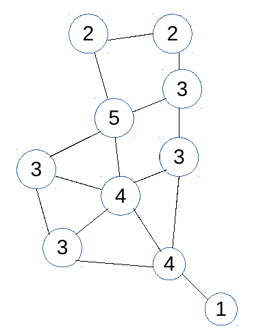
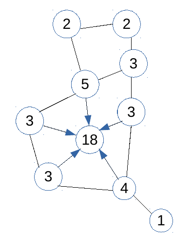
Fig. 1: (a) Initial TNF values (b) Iteration 1 of $\mathit{SI}$.

Dahm et al.[Dahm et al., 2015] define this index as a sum of TNF values of adjacent or neighboring nodes.

$$\mathit{SI}_{i}(v)=\begin{cases}feature(v)&if~{}i=0\\ \sum\limits_{u}\mathit{SI}_{i-1}(u)&otherwise\end{cases}$$ (3)

where u is the node adjacent to v, $feature(v)$ is initial TNF, $d$ of a node. Fig. 1 shows the evaluation of $\mathit{SI}_{2}$ from $\mathit{SI}_{1}$ in one iteration. For every node $p$ in G, we calculated two iterations of $\mathit{SI}$ and placed them in $\mathit{SI}$ vector $\mathscr{V}(p)$ = ($\mathit{SI}_{1}$, $\mathit{SI}_{2}$, $\mathit{SI}_{3}$). This captures various levels of local structural information.
We defined

$$\zeta_{ij}=||\mathscr{V}(p_{i})-\mathscr{V}(p_{j})||$$ (4)

5.1 Generalized Framework for Affinity definition

In order to enhance the affinity between any two data points $p_{i}$, $p_{j}$, we propose the following generalized framework:

$$A_{ij}^{\prime}=A_{ij}*K^{1}_{ij}*K^{2}_{ij}*K^{3}_{ij}$$ (5)

where $A_{ij}$ is the traditional affinity, $K^{1}(.)$ represents density information. $K^{2}(.)$ represents local similarity in terms of spatial nearness. $K^{3}(.)$ represents local structural similarity, and $A_{ij}^{\prime}$ is defined as product of these individual kernels.
Multiple local features are incorporated using various kernels. In this method there is a risk of over-fitting. Unnecessary information might lead to ineffective affinity metric definition as shown in some of the results in Sec 7. According to the dataset considered, appropriate local features have to be incorporated into the generalized definition of metric.

6 Proposed Affinity matrix creation

The steps in affinity matrix creation employed in our method are:

1. Model the datapoints as a graph G as explained in Sec 4.1.

2. Let $\tau_{ij}=D(p_{i},p_{j})$ denote any standard distance(eg. Euclidean) defined over the given data points.

3. At each node p, calculate the following TNFs:

   1. Degree of node ($d_{p}$)

   2. Clustering coefficient ($\phi_{p}$)

   3. SI vector $\mathscr{V}_{p}$=($\mathit{{SI}_{1}}$, $\mathit{{SI}_{2}}$, $\mathit{{SI}_{3}}$)

4. We defined the similarity $A_{ij}$ between any two nodes $p_{i},p_{j}$ as:

   $$A_{ij}=\beta_{ij}*\bigg{(}1+\frac{1}{1+log(1+\zeta_{ij})}\bigg{)}\vspace{.07cm}$$ (6)

   where

   $$\beta_{ij}=exp\bigg{(}\frac{-\tau_{ij}^{2}*\delta_{ij}}{2\sigma^{2}}\bigg{)}*\eta_{ij}$$ (7)

   where $\delta_{ij}=abs(\phi_{i}-\phi_{j}$), $\eta_{ij}$ is the number of common points between $\aleph(p_{i}),\aleph(p_{j})$, and $\sigma$ is the scale parameter of the Gaussian function.

Elucidating the saliency features of $A_{ij}$, the expression of $A_{ij}$ captures local density, common neighbors, and Summation Indices in the following way.
In Eq. (7), the expression for $\beta_{ij}$ incorporates spatial nearness in the form of $\eta_{ij}$. We also note that the exponential term of $\beta_{ij}$ involves the traditional distance $\tau_{ij}$ scaled with $\delta_{ij}$. Thus for points with similar density, the effective affinity will be pronounced.
The second term in Eq. (6) has $\zeta_{ij}$ as the argument of log function in the denominator. Since $\zeta_{ij}$ is the difference between the local structural information of $p_{i},p_{j}$, the affinity increases with decrease in $\zeta_{ij}$.
Thus in the proposed affinity measure $A_{ij}$, we are able to strengthen or penalize the traditional affinity according to local topological graph properties. This enables our method to perform better across different types of datasets.

6.1 Effectiveness of TNFs

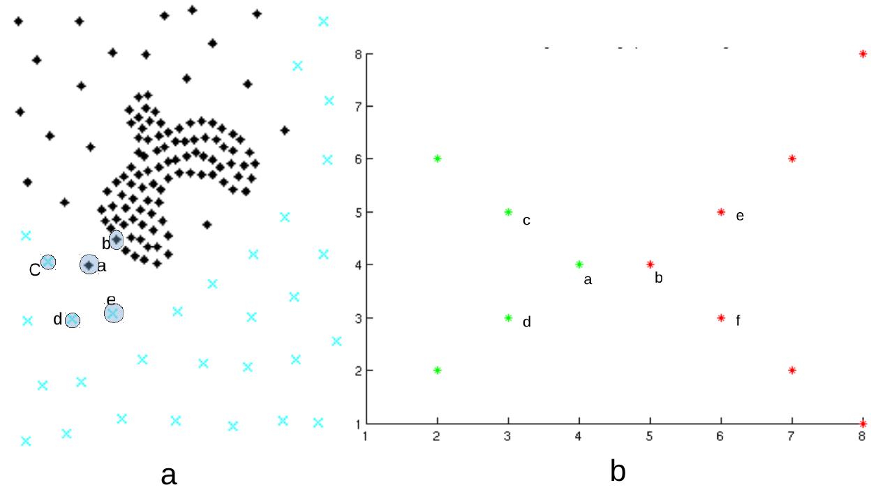
Fig. 2: (a) Dataset 1 (b) Dataset 2

Table 1: Comparison of methods using ARI metric on Shape datasets

Affinity	Aff1	TNF1	TNF2
A(a,b)	9.66e-92	3.71e-32	3.99e-32
A(a,c)	6.65e-158	2.38e-44	2.56e-44
A(a,d)	3.85e-138	3.09e-39	3.33e-39
A(a,e)	5.88e-142	2.75e-28	2.97e-28

As part of our first experiment, we considered a part of Compound dataset[Lichman, 2013] shown in Fig. 2(a), to highlight the working of our method. Consider points ‘a’, ‘b’, ‘c’, ‘d’, ‘e’ from the figure. NJW[Ng et al., 2002] wrongly assigns point ‘a’ into the cluster in the center whereas our technique classifies it correctly( Fig. 3).
The various types of affinities between ‘a’ and surrounding points ‘b’,‘c’,‘d’,‘e’ are shown in Table 1. Aff1 refers to the Gaussian kernel distance( $\hat{A}_{ij}$). TNF1 is the affinity proposed in Eq. (7), which includes local density and common neighbor parameters. TNF2 refers to the affinity proposed in Eq. (6), which includes structural properties along with density and common neighbor properties.
From the Table 1, we see that in the case of Aff1: A(a,b) $>$ A(a,d) $>$ A(a,e) $>$ A(a,c). This led to wrong clustering of point ‘a’. Whereas in case of affinity TNF2 : A(a,e) $>$ A(a,b) $>$ A(a,d) $>$ A(a,c). This led to a correct clustering of point ‘a’.
The second experiment we conducted is on data given in Fig. 2(b). The affinities between points ‘a’, ‘b’ are listed in Table 2. From the table we can see that the Aff1 between points is same but the values of TNF2 between points is different. This is to show that even when the Gaussian kernel distance between points does not show variation, structural properties can differentiate between points.
This shows that our method which incorporates density and structural properties will lead to effective similarity between points.

Table 2: Comparison of methods using ARI metric on Shape datasets

Affinity	A(a,b)	A(a,c)	A(a,d)	A(b,e)	A(b,f)
Aff1	8.2	8.2	8.2	8.2	8.2
TNF2	.6402	.2262	.2262	1448	.2260

7 Results and Analysis

In this section, we demonstrate the results of proposed method applied on three different types of datasets. The comparative results with respect to the state of the art existing techniques demonstrate the effectiveness of our method.
For experimentation, from Eq.(6) we considered two cases:
Case 1(TNF1): $A_{ij}=\beta_{ij}$
Here we retained only the first term which accounts for local density and spatial nearness in the data.
Case 2(TNF2): $A_{ij}$, as defined in Eq. (6), which incorporates structural information in addition to $\beta_{ij}$.
We observed that the structural similarity term plays an important role in some cases. For example in the case of Wine dataset (Table 6), by including structural similarity, we obtained clear improvement over TNF1. Whereas in case of Glass, Iris, etc. the improvement is not significant.
However compared to other methods, SC by NJW[Ng et al., 2002], and self-tuning(ST) SC proposed by Perona and Manor[Zelnik Manor and Perona, 2004], and Common nearest neighbors based method given by Zhang et al.[Zhang et al., 2011] both TNF1 and TNF2 have done well. We considered Self Tuning with local scaling[Zelnik Manor and Perona, 2004], which in general performs better than the other variation proposed by the same authors.
In our experiments we used three types of metrics for comparison: Adjusted Rand Index(ARI)[Rand, 1971], Normalized Mutual Information(NMI)[Strehl and Ghosh, 2003], Clustering Error(CE)[Jordan and Bach, 2004]. The values of NMI and ARI approach unity as the result goes closer to the ground truth. The metric CE represents the error in clustering that tends to null as the clustering accuracy increases.

7.1 Shape datasets

In the 2D shape datasets[Lichman, 2013], we considered six examples for our experiments namely, Compound, Aggre, Flame, Jain, Pathbased, and Spiral. The datasets present challenges such as varying density, connectedness of data etc. Some of the sample results are displayed in Table 3.
In the current set of experiments, the $\sigma$ value is chosen empirically. We experimented with $\sigma$ varying from .01 to 10 with an interval of .01. Selection of optimal sigma for spectral clustering is an open problem and a few methods have been proposed in the literature[Zhang et al., 2010; Gu and Wang, 2009]. We note that in all cases both TNF1 and TNF2 are performing better. TNF2 does not show significant improvement over TNF1.

Fig. 3: First column shows original datasets, second column shows results of NJW. Third column is the result of CNN based method. Fourth column is the result of the proposed algorithm

Table 3: Comparison of methods using ARI metric on Shape datasets

			Datasets
Method	Comp	Aggre	Flame	Jain	Path	Spiral
NCUTS	0.9405	0.9869	1	1	0.7143	1
ST	0.5184	0.9642	0.625	0.9444	0.5138	0.0781
CNN	0.8955	0.9833	0.9667	1	0.7187	1
TNF1	0.9972	1	1	1	0.9899	1
TNF2	0.9972	1	1	1	1	1

Table 4: Comparison of methods using NMI metric on Shape datasets

			Datasets
Method	Comp	Aggre	Flame	Jain	Path	Spiral
NCUTS	0.9171	0.9824	1	1	0.7825	1
ST	0.7632	0.9661	0.564	0.8961	0.5869	0.1716
CNN	.9120	0.9808	0.9269	1	0.7728	1
TNF1	0.9924	1	1	1	0.9829	1
TNF2	0.9924	1	1	1	1	1

Table 5: Comparison of methods using CE metric on Shape datasets

			Datasets
Method	Comp	Aggre	Flame	Jain	Path	Spiral
NCUTS	0.0526	0.0063	0	0	0.1133	0
ST	0.3559	0.0165	0.1042	0.0134	0.2133	0.4808
CNN	0.0702	0.0076	0.0083	0	0.1100	0
TNF1	0.0025	0	0	0	0.0033	0
TNF2	0.0025	0	0	0	0	0

7.2 Real datasets

We considered UCI real datasets([Lichman, 2013]) as second type of dataset. These datasets are collected from real scenarios and have varied number of features and distributions. Results of TNF1, TNF2 in comparison with other SC methods are given in Tables 6, 7, 8. From the results shown in Table 6, we see that TNF2 shows improvement over TNF1 in Wine, Glass and Iris datasets. In case of Ion dataset, the result remains same. In case of Sonar dataset, TNF1 is better than TNF2 with respect to ARI metric. The structure of the dataset then determines which TNFs help in creating effective affinity matrix.

Table 6: Comparison of methods using ARI metric on UCI datasets

			Datasets
Methods	Wine	Glass	Iris	Ion	Sonar
NCUTS	0.4127	0.2876	0.8161	0.6647	0.0630
ST	0.319	0.2352	0.7580	0.2184	0
CNN	0.9149	0.2806	0.7592	0.6926	0.0289
TNF1	0.7782	0.3559	0.8683	0.7020	0.1438
TNF2	0.9471	0.3575	0.8858	0.7020	0.1224

Table 7: Comparison of methods using NMI metric on UCI datasets

			Datasets
Methods	Wine	Glass	Iris	Ion	Sonar
SC	0.4554	0.4670	0.8058	0.5463	0.0995
ST	0.395	0.4143	0.7856	0.2214	0.0030
CNN	0.8926	0.4406	0.8058	0.5820	0.0615
TNF1	0.7696	0.4943	0.8572	0.6116	0.1757
TNF2	0.9276	0.5035	0.8705	0.6116	0.1946

Table 8: Comparison of methods using CE metric on UCI datasets

			Datasets
Methods	Wine	Glass	Iris	Ion	Sonar
SC	0.2809	0.4393	0.0667	0.0912	0.3702
ST	0.4440	0.5373	0.0930	0.2650	0.4760
CNN	0.0281	0.4533	0.0933	0.0826	0.4087
TNF1	0	0.3645	0.0467	0.0798	0.3077
TNF2	0	0.3598	0	0.0800	0.3221

Table 9: Comparison of methods using ARI metric on MNSIT datasets

		Datasets
Methods	{0,8}	{3,5,8}	{1,2,3,4}
SC	1	0.5657	0.3740
ST	1	0.4535	0.2297
CNN	1	0.5682	0.33102
TNF1	1	0.8159	0.6340

Table 10: Comparison of methods using NMI metric on MNSIT datasets

		Datasets
Methods	{0,8}	{3,5,8}	{1,2,3,4}
SC	1	0.7502	0.6216
ST	1	0.6570	0.5221
CNN	1	0.7545	0.6325
TNF1	1	0.7802	0.6835

Table 11: Comparison of methods using CE metric on MNSIT datasets

		Datasets
Methods	{0,8}	{3,5,8}	{1,2,3,4}
SC	0	0.3367	0.4050
ST	0	0.4533	0.6650
CNN	0	0.3350	0.5013
TNF1	0	.0667	.1800

7.3 Handwritten datasets

MNIST dataset given by lecun et al.[LeCun et al., 1998] is a handwritten digits database. It has a training set of 60,000 examples and test set of 10,000 samples. For each of the ten digits, there is a test set of 1000 samples. All the samples are images of size 28x28.
For our experiments, we considered 200 samples of each digit. We tested our method on some of challenging test cases such as {0,8}, {3,5,8}, {1,2,3,4}. We employed TNF1 for this dataset. Tables 9, 10, 11 summarize the results that again reiterate the greater efficacy of our technique.

8 Conclusion

Traditionally, in a SC algorithm, the pairwise similarity between data points is estimated using a Gaussian kernel function. In this work, we proposed a novel similarity measure based on local properties. Properties, such as local neighborhood, local density information, and local structure were estimated using TNFs and were incorporated into the construction of pairwise affinity. Using topological graph properties, we were able to enhance or penalize the pairwise similarity. Our experiments on synthetic, real and handwriting datasets show that proposed TNF based technique improved the effectiveness of SC. In our future work, we would like to adapt this framework for different applications such as Image segmentation etc. The framework can also be strengthened by assimilating more topological node features such as Listing index, Tree index [Dahm et al., 2015].

References

- Beauchemin [2015] Beauchemin, M., 2015. A density-based similarity matrix construction for spectral clustering. Neurocomputing 151, 835–844.
- Cordella et al. [2004] Cordella, L.P., Foggia, P., Sansone, C., Vento, M., 2004. A (sub) graph isomorphism algorithm for matching large graphs. Pattern Analysis and Machine Intelligence, IEEE Transactions on 26, 1367–1372.
- Dahm et al. [2015] Dahm, N., Bunke, H., Caelli, T., Gao, Y., 2015. Efficient subgraph matching using topological node feature constraints. Pattern Recognition 48, 317–330.
- Diao et al. [2015] Diao, C., Zhang, A.H., Wang, B., 2015. Spectral clustering with local projection distance measurement. Mathematical Problems in Engineering 2015.
- Gu and Wang [2009] Gu, R., Wang, J., 2009. An improved spectral clustering algorithm based on neighbour adaptive scale, in: Business Intelligence and Financial Engineering, 2009. BIFE’09. International Conference on, IEEE. pp. 233–236.
- Jordan and Bach [2004] Jordan, F., Bach, F., 2004. Learning spectral clustering. Adv. Neural Inf. Process. Syst 16, 305–312.
- LeCun et al. [1998] LeCun, Y., Bottou, L., Bengio, Y., Haffner, P., 1998. Gradient-based learning applied to document recognition. Proceedings of the IEEE 86, 2278–2324. URL: http://yann.lecun.com/exdb/mnist/.
- Lichman [2013] Lichman, M., 2013. UCI machine learning repository. URL: http://archive.ics.uci.edu/ml.
- Ng et al. [2002] Ng, A.Y., Jordan, M.I., Weiss, Y., 2002. On spectral clustering: Analysis and an algorithm. Advances in neural information processing systems 2, 849–856.
- Rand [1971] Rand, W.M., 1971. Objective criteria for the evaluation of clustering methods. Journal of the American Statistical association 66, 846–850.
- Shi and Malik [2000] Shi, J., Malik, J., 2000. Normalized cuts and image segmentation. Pattern Analysis and Machine Intelligence, IEEE Transactions on 22, 888–905.
- Sorlin and Solnon [2008] Sorlin, S., Solnon, C., 2008. A parametric filtering algorithm for the graph isomorphism problem. Constraints 13, 518–537.
- Strehl and Ghosh [2003] Strehl, A., Ghosh, J., 2003. Cluster ensembles: a knowledge reuse framework for combining multiple partitions. The Journal of Machine Learning Research 3, 583–617.
- Yang et al. [2011] Yang, P., Zhu, Q., Huang, B., 2011. Spectral clustering with density sensitive similarity function. Knowledge-Based Systems 24, 621–628.
- Yang et al. [2013] Yang, Y., Wang, Y., Cheung, Y.M., 2013. Kernel fuzzy similarity measure-based spectral clustering for image segmentation, in: Human-Computer Interaction. Towards Intelligent and Implicit Interaction. Springer, pp. 246–253.
- Zelnik Manor and Perona [2004] Zelnik Manor, L., Perona, P., 2004. Self tuning spectral clustering, in: Advances in neural information processing systems, pp. 1601–1608. URL: http://www.vision.caltech.edu/lihi/Demos/SelfTuningClustering.html.
- Zhang et al. [2011] Zhang, X., Li, J., Yu, H., 2011. Local density adaptive similarity measurement for spectral clustering. Pattern Recognition Letters 32, 352–358.
- Zhang et al. [2010] Zhang, Y., Zhou, J., Fu, Y., 2010. Spectral clustering algorithm based on adaptive neighbor distance sort order, in: Information Sciences and Interaction Sciences (ICIS), 2010 3rd International Conference on, IEEE. pp. 444–447.