Sufficient conditions for the value function and optimal strategy to be even and quasi-convex

Abstract

Sufficient conditions are identified under which the value function and the optimal strategy of a Markov decision process (MDP) are even and quasi-convex in the state. The key idea behind these conditions is the following. First, sufficient conditions for the value function and optimal strategy to be even are identified. Next, it is shown that if the value function and optimal strategy are even, then one can construct a “folded MDP” defined only on the non-negative values of the state space. Then, the standard sufficient conditions for the value function and optimal strategy to be monotone are “unfolded” to identify sufficient conditions for the value function and the optimal strategy to be quasi-convex. The results are illustrated by using an example of power allocation in remote estimation.

I Introduction

I-A Motivation

Markov decision theory is often used to identify structural or qualitative properties of optimal strategies. Examples include control limit strategies in machine maintenance [1, 2], threshold-based strategies for executing call options [3, 4], and monotone strategies in queueing systems [5, 6]. In all of these models, the optimal strategy is monotone in the state, i.e., if $x>y$ then the action chosen at $x$ is greater (or less) than or equal to the action chosen at $y$. Motivated by this, general conditions under which the optimal strategy is monotone in scalar-valued states are identified in [7, 8, 9, 10, 11, 12]. Similar conditions for vector-valued states are identified in [13, 14, 15]. General conditions under which the value function is increasing and convex are established in [16].

Most of the above results are motivated by queueing models where the state is the queue length which takes non-negative values. However, for typical applications in systems and control, the state takes both positive and negative values. Often, the system behavior is symmetric for positive and negative values, so one expects the optimal strategy to be even. Thus, for such systems, a natural counterpart of monotone functions are even and quasi-convex (or quasi-concave) functions. In this paper, we identify sufficient conditions under which the value function and optimal strategy are even and quasi-convex.

As a motivating example, consider a remote estimation system in which a sensor observes a Markov process and decides whether to transmit the current state of the Markov process to a remote estimator. There is a cost or constraint associated with transmission. When the transmitter does not transmit or when the transmitted packet is dropped due to interference, the estimator generates an estimate of the state of the Markov process based on the previously received states. The objective is to choose transmission and estimation strategies that minimize either the expected distortion and cost of communication or minimize expected distortion under the transmission constraint. Variations of such models have been considered in [17, 18, 19, 20, 21, 22, 23].

In such models, the optimal transmission and estimation strategies are identified in two steps. In the first step, the joint optimization of transmission and estimation strategies is investigated and it is established that there is no loss of optimality in restricting attention to estimation strategies of a specific form. In the second step, estimation strategies are restricted to the form identified in the first step and the structure of the best response transmission strategies is established. In particular, it is shown that the optimal transmission strategies are even and quasi-convex. Currently, in the literature these results are established on a case by case basis. For example, see [18, Theorem 1],  [20, Theorem 3], [24, Theorem 1], [21, Theorem 1] among others.

In this paper, we identify sufficient conditions for the value functions and optimal strategy of a Markov decision process to be even and quasi-convex. We then consider a general model of remote estimation and verify these sufficient conditions.

I-B Model and problem formulation

Consider a Markov decision process (MDP) with state space $\mathds{X}$ (which is either $\mathds{R}$, the real line, or a symmetric subset of the form $[-a,a]$) and action space $\mathds{U}$ (which is either a countable set or a compact subset of reals).

Let $X_{t}\in\mathds{X}$ and $U_{t}\in\mathds{U}$ denote the state and action at time $t$. The initial state $X_{1}$ is distributed according to the probability density function $\mu$ and the state evolves in a controlled Markov manner, i.e., for any Borel measurable subset $A$ of $\mathds{X}$,

$$\mathds{P}(X_{t+1}\in A\mid X_{1:t}=x_{1:t},U_{1:t}=u_{1:t})\\ =\mathds{P}(X_{t+1}\in A\mid X_{t}=x_{t},U_{t}=u_{t}),$$

where $x_{1:t}$ is a short hand notation for $(x_{1},\dots,x_{t})$ and a similar interpretation holds for $u_{1:t}$. We assume that there exists a (time-homogeneous) controlled transition density $p(y|x;u)$ which is continuous in $y$ for any $x\in\mathds{X}$ and $u\in\mathds{U}$ and for any Borel measurable subset $A$ of $\mathds{X}$,

$$\mathds{P}(X_{t+1}\in A\mid X_{t}=x,U_{t}=u)=\int_{A}p(y|x;u)dy.$$

We use $p(u)$ to denote transition density corresponding to action ${u\in\mathds{U}}$.

The system operates for a finite horizon $T$. For any time $t\in\{1,\dots,{T-1}\}$, a measurable and lower semi-continuous function $c_{t}\colon\mathds{X}\times\mathds{U}\to\mathds{R}$ denotes the instantaneous cost at time $t$ and at the terminal time $T$ a measurable and lower semi-continuous function $c_{T}\colon\mathds{X}\to\mathds{R}$ denotes the terminal cost.

The actions at time $t$ are chosen according to a Markov strategy $g_{t}$, i.e.,

$$U_{t}=g_{t}(X_{t}),\quad t\in\{1,\dots,{T-1}\}.$$

The objective is to choose a decision strategy $\mathbf{g}\coloneqq(g_{1},\dots,g_{T-1})$ to minimize the expected total cost

$$J_{T}(\mathbf{g})\coloneqq\mathds{E}^{g}\Big{[}\sum_{t=1}^{T-1}c_{t}(X_{t},U_{t})+c_{T}(X_{T})\Big{]}.$$ (1)

We denote such an MDP by $(\mathds{X},\mathds{U},p,c_{t})$.

From Markov decision theory [25], we know that an optimal strategy is given by the solution of the following dynamic program. Recursively define value functions $V_{t}\colon\mathds{X}\to\mathds{R}$ and value-action functions $Q_{t}\colon\mathds{X}\times\mathds{U}\to\mathds{R}$ as follows: for all $x\in\mathds{X}$ and $u\in\mathds{U}$,

$$V_{T}(x) =c_{T}(x),$$ (2)

and for $$t\in\{{T-1},\dots,1\}$$,

$$Q_{t}(x,u) =c_{t}(x,u)+\mathds{E}[V_{t+1}(X_{t+1})\mid X_{t}=x,U_{t}=u]$$

$$=c_{t}(x,u)+\int_{\mathds{X}}p(y|x;u)V_{t+1}(y)dy,$$ (3)

$$V_{t}(x) =\min_{u\in\mathds{U}}Q_{t}(x,u).$$ (4)

Then, a strategy $\mathbf{g}^{*}=(g^{*}_{1},\dots,g^{*}_{T-1})$ defined as

$$g^{*}_{t}(x)\in\arg\min_{u\in\mathds{U}}Q_{t}(x,u)$$

is optimal. To avoid ambiguity when the arg min is not unique, we pick

$$g_{t}^{*}(x)=\begin{dcases}\max\big{\{}v\in\arg\min_{u\in\mathds{U}}Q_{t}(x,u)\big{\}},&\hbox{if $x\geq 0$}\\ \min\big{\{}v\in\arg\min_{u\in\mathds{U}}Q_{t}(x,u)\big{\}},&\hbox{if $x<0$}.\end{dcases}$$ (5)

Let $\mathds{X}_{\geq 0}$ and $\mathds{X}_{>0}$ denote the sets $\{x\in\mathds{X}:x\geq 0\}$ and $\{x\in\mathds{X}:x>0\}$. We say that a function $f\colon\mathds{X}\to\mathds{R}$ is even and quasi-convex if it is even and for $x,x^{\prime}\in\mathds{X}_{\geq 0}$ such that $x<x^{\prime}$, we have that $f(x)\leq f(x^{\prime})$. The main contribution of this paper is to identify sufficient conditions under which $V_{t}$ and $g^{*}_{t}$ are even and quasi-convex.

I-C Main result

Definition 1

For a given $u\in\mathds{U}$, we say that a controlled transition density $p(u)$ on $\mathds{X}\times\mathds{X}$ is even if for all $x,y\in\mathds{X}$, $p(y|x;u)=p(-y|{-x};u)$. _□

Our main result is the following.

Theorem 1

Given an MDP $(\mathds{X},\mathds{U},p,c_{t})$, define for $x,y\in\mathds{X}_{\geq 0}$ and $u\in\mathds{U}$,

$$S(y|x;u)\coloneqq 1-\int_{A_{y}}[p(z|x;u)+p(-z|x;u)]dz,$$ (6)

where $A_{y}=\{z\in\mathds{X}:z<y\}$. Consider the following conditions:

1. $c_{T}(\cdot)$ is even and quasi-convex and for $t\in\{1,\dots,{T-1}\}$ and $u\in\mathds{U}$, $c_{t}(\cdot,u)$ is even and quasi-convex.

2. For all $u\in\mathds{U}$, $p(u)$ is even.

3. For all $u\in\mathds{U}$ and $y\in\mathds{X}_{\geq 0}$, $S(y|x;u)$ is increasing for $x\in\mathds{X}_{\geq 0}$.

4. For $t\in\{1,\dots,T-1\}$, $c_{t}(x,u)$ is submodular in $(x,u)$ on $\mathds{X}_{\geq 0}\times\mathds{U}$.

5. For all $y\in\mathds{X}_{\geq 0}$, $S(y|x;u)$ is submodular in $(x,u)$ on $\mathds{X}_{\geq 0}\times\mathds{U}$.

Then, under (C1)–(C3), $V_{t}(\cdot)$ is even and quasi-convex for all $t\in\{1,\dots,T\}$ and under (C1)–(C5), $g^{*}_{t}(\cdot)$ is even and quasi-convex for all $t\in\{1,\dots,T-1\}$. _□

The main idea of the proof is as follows. First, we identify conditions under which the value function and optimal strategy of an MDP are even. Next, we show that if we construct an MDP by “folding” the transition density, then the “folded MDP” has the same value function and optimal strategy as the original MDP for non-negative values of the state. Finally, we show that if we take the sufficient conditions under which the value function and the optimal strategy of the folded MDP are increasing and “unfold” these conditions back to the original model, we get conditions (C1)–(C5) above. The details are given in Sections II and III.

II Even MDPs and folded representations

We say that an MDP is even if for every $t$ and every $u\in\mathds{U}$, $V_{t}(x)$, $Q_{t}(x,u)$ and $g^{*}_{t}(x)$ are even in $x$. We start by identifying sufficient conditions for an MDP to be even.

II-A Sufficient conditions for MDP to be even

Proposition 1

Suppose an MDP $(\mathds{X},\mathds{U},p,c_{t})$ satisfies the following properties:

(A1)

$c_{T}(\cdot)$ is even and for every $t\in\{1,\cdots,T-1\}$ and $u\in\mathds{U}$, $c_{t}(\cdot,u)$ is even.

(A2)

For every $u\in\mathds{U}$, the transition density $p(u)$ is even.

Then, the MDP is even. _□

Proof

We proceed by backward induction. $V_{T}(x)=c_{T}(x)$ which is even by (A1). This forms the basis of induction. Now assume that $V_{t+1}(x)$ is even in $x$. For any $u\in\mathds{U}$, we show that $Q_{t}(x,u)$ is even in $x$. Consider,

$$\hskip-20.00003ptQ_{t}(-x,u)=c_{t}(-x,u)+\int_{\mathds{X}}p(y|{-x};u)V_{t+1}(y)dy$$

$$\hskip-20.00003pt\stackrel{{\scriptstyle(a)}}{{=}}c_{t}(x,u)+\int_{\mathds{X}}p({-z}|{-x};u)V_{t+1}(-z)dz$$

$$\hskip-20.00003pt\stackrel{{\scriptstyle(b)}}{{=}}c_{t}(x,u)+\int_{\mathds{X}}p(z|x;u)V_{t+1}(z)dz=Q_{t}(x,u)$$

where $(a)$ follows from (A1), a change of variables $y=-z$, and the fact that $\mathds{X}$ is a symmetric interval; and $(b)$ follows from (A2) and the induction hypothesis that $V_{t+1}(\cdot)$ is even. Hence, $Q_{t}(\cdot,u)$ is even.

Since $Q_{t}(\cdot,u)$ is even, Eqs. (4) and (5) imply that $V_{t}$ and $g^{*}_{t}$ are also even. Thus, the result is true for time $t$ and, by induction, true for all time $t$. _■

II-B Folding operator for distributions

We now show that if the value function is even, we can construct a “folded” MDP with state-space $\mathds{X}_{\geq 0}$ such that the value function and optimal strategy of the folded MDP match that of the original MDP on $\mathds{X}_{\geq 0}$. For that matter, we first define the following:

Definition 2 (Folding Operator)

Given a probability density $\pi$ on $\mathds{X}$, the folding operator $\mathcal{F}\pi$ gives a density $\tilde{\pi}$ on $\mathds{X}_{\geq 0}$ such that for any $x\in\mathds{X}_{\geq 0}$, $\tilde{\pi}(x)=\pi(x)+\pi(-x)$. _□

As an immediate implication, we have the following:

Lemma 1

If $f:\mathds{X}\to\mathds{R}$ is even, then for any probability distribution $\pi$ on $\mathds{X}$ and $\tilde{\pi}=\mathcal{F}\pi$, we have

$$\int_{\mathds{X}}f(x)\pi(x)dx=\int_{\mathds{X}_{\geq 0}}f(x)\tilde{\pi}(x)dx.$$

_□

Now, we generalize the folding operator to transition densities.

Definition 3

Given a transition density $p$ on $\mathds{X}\times\mathds{X}$, the folding operator $\mathcal{F}p$ gives a transition density $\tilde{p}$ on $\mathds{X}_{\geq 0}\times\mathds{X}_{\geq 0}$ such that for any $x,y\in\mathds{X}_{\geq 0}$, $\tilde{p}(y|x)=p(y|x)+p(-y|x).$ _□

Definition 4 (Folded MDP)

Given an MDP $(\mathds{X},\mathds{U},p,c_{t})$, define the folded MDP as $(\mathds{X}_{\geq 0},\mathds{U},\tilde{p},c_{t})$, where for all $u\in\mathds{U}$, $\tilde{p}(u)=\mathcal{F}p(u)$. _□

Let $\tilde{Q}_{t}$ and $\tilde{V}_{t}$ and $\tilde{g}^{*}_{t}$ denote respectively the value-action function, the value function, and the optimal strategy of the folded MDP. Then, we have the following.

Proposition 2

If the MDP $(\mathds{X},\mathds{U},p,c_{t})$ is even, then for any $x\in\mathds{X}$ and $u\in\mathds{U}$,

$$Q_{t}(x,u)=\tilde{Q}_{t}(|x|,u),\quad V_{t}(x)=\tilde{V}_{t}(|x|),\quad g^{*}_{t}(x)=\tilde{g}^{*}_{t}(|x|).$$ (7)

_□

Proof

We proceed by backward induction. For $x\in\mathds{X}$ and $\tilde{x}\in\mathds{X}_{\geq 0}$, $V_{T}(x)=c_{T}(x)$ and $\tilde{V}_{T}(\tilde{x})=c_{T}(\tilde{x})$. Since $V_{T}(\cdot)$ is even, $V_{T}(x)=V_{T}(|x|)=\tilde{V}_{T}(|x|)$. This is the basis of induction. Now assume that for all $x\in\mathds{X}$, $V_{t+1}(x)=\tilde{V}_{t+1}(|x|)$. Consider $x\in\mathds{X}_{\geq 0}$ and $u\in\mathds{U}$. Then we have

$$\hskip-20.00003ptQ_{t}(x,u)=c_{t}(x,u)+\int_{\mathds{X}}p(y|x;u)V_{t+1}(y)dy$$

$$\hskip-20.00003pt\stackrel{{\scriptstyle(a)}}{{=}}c_{t}(x,u)+\int_{\mathds{X}_{\geq 0}}\tilde{p}(y|x;u)V_{t+1}(y)dy$$

$$\hskip-20.00003pt\stackrel{{\scriptstyle(b)}}{{=}}c_{t}(x,u)+\int_{\mathds{X}_{\geq 0}}\tilde{p}(y|x;u)\tilde{V}_{t+1}(y)dy=\tilde{Q}_{t}(x,u),$$

where $(a)$ uses Lemma 1 and that $V_{t+1}$ is even and $(b)$ uses the induction hypothesis.

Since the $Q$-functions match for $x\in\mathds{X}_{\geq 0}$, equations (4) and (5) imply that the value functions and the optimal strategies also match on $\mathds{X}_{\geq 0}$, i.e., for $x\in\mathds{X}_{\geq 0}$,

$$V_{t}(x)=\tilde{V}_{t}(x)\quad\text{and}\quad g^{*}_{t}(x)=\tilde{g}^{*}_{t}(x).$$

Since $V_{t}$ and $g^{*}_{t}$ are even, we get that (7) is true at time $t$. Hence, by principle of induction, it is true for all $t$. _■

III Monotonicity of the value function and the optimal strategy

We have shown that under (A1) and (A2) the original MDP is equivalent to a folded MDP with state-space $\mathds{X}_{\geq 0}$. Thus, we can use standard conditions to determine when the value function and the optimal strategy of the folded MDP are monotone. Translating these conditions back to the original model, we get the sufficient conditions for the original model.

III-A Monotonicity of the value function

The results on monotonicity of value functions rely on the notion of stochastic monotonicity.

Given a transition density $p$ defined on $\mathds{X}$, the cumulative transition distribution function $P$ is defined as

$$P(y|x)=\int_{A_{y}}p(z|x)dz,\quad\hbox{where }A_{y}=\{z\in\mathds{X}:z<y\}.$$

Definition 5 (Stochastic Monotonicity)

A transition density $p$ on $\mathds{X}$ is said to be stochastically monotone increasing if for every $y\in\mathds{X}$, the cumulative distribution function $P(y|x)$ corresponding to $p$ is decreasing in $x$. _□

Proposition 3

Suppose the folded MDP $(\mathds{X}_{\geq 0},\mathds{U},\tilde{p},c_{t})$ satisfies the following:

(B1)

$c_{T}(x)$ is increasing in $x$ for $x\in\mathds{X}_{\geq 0}$; for any $t\in\{1,\dots,T-1\}$ and $u\in\mathds{U}$, $c_{t}(x,u)$ is increasing in $x$ for $x\in\mathds{X}_{\geq 0}$.

(B2)

For any $u\in\mathds{U}$, $\tilde{p}(u)$ is stochastically monotone increasing.

Then, for any $t\in\{1,\dots,T\}$, $\tilde{V}_{t}(x)$ is increasing in $x$ for $x\in\mathds{X}_{\geq 0}$. _□

A version of this proposition when $\mathds{X}$ is a subset of integers is given in [8, Theorem 4.7.3]. The same proof argument also works when $\mathds{X}$ is a subset of reals.

Recall the definition of $S$ given in (6). (B2) is equivalent to the following:

(B2’)

For every $u\in\mathds{U}$ and $x,y\in\mathds{X}_{\geq 0}$, $S(y|x;u)$ is increasing in $x$.

An immediate consequence of Propositions 1, 2, and 3 is the following:

Corollary 1

Under (A1), (A2), (B1), and (B2) (or (B2’)), the value functions $V_{t}(\cdot)$ is even and quasi-convex. _□

Remark 1

Note that (A1) and (B1) are equivalent to (C1), (A2) is same as (C2), and (B2) (or equivalently, (B2’)) is equivalent to (C3). Thus, Corollary 1 proves the first part of Theorem 1. _□

III-B Monotonicity of the optimal strategy

Now we state sufficient conditions under which the optimal strategy is increasing. These results rely on the notion of submodularity.

Definition 6 (Submodular function)

A function $f\colon\mathds{X}\times\mathds{U}\to\mathds{R}$ is called submodular if for any $x,y\in\mathds{X}$ and $u,v\in\mathds{U}$ such that $x\geq y$ and $u\geq v$, we have

$$f(x,u)+f(y,v)\leq f(x,v)+f(y,u).$$

_□

An equivalent characterization of submodularity is that

$$f(y,u)-f(y,v)\geq f(x,u)-f(x,v),$$

$$\implies f(x,v)-f(y,v)\geq f(x,u)-f(y,u),$$

which implies that the differences in one variable are decreasing in the other.

Proposition 4

Suppose that in addition to (B1) and (B2) (or (B2’)), the folded MDP $(\mathds{X}_{\geq 0},\mathds{U},\tilde{p},c_{t})$ satisfies the following property:

(B3)

For all $t\in\{1,\dots,T-1\}$, $c_{t}(x,u)$ is submodular in $(x,u)$ on $\mathds{X}_{\geq 0}\times\mathds{U}$.

(B4)

For all $y\in\mathds{X}_{\geq 0}$, $S(y|x;u)$ is submodular in $(x,u)$ on $\mathds{X}_{\geq 0}\times\mathds{U}$, where $S(y|x;u)$ is defined in (6).

Then, for every $t\in\{1,\cdots,T-1\}$, the optimal strategy $\tilde{g}^{*}_{t}(x)$ is increasing in $x$ for $x\in\mathds{X}_{\geq 0}$. _□

A version of this proposition when $\mathds{X}$ is a subset of integers is given in [8, Theorem 4.7.4]. The same proof argument also works when $\mathds{X}$ is a subset of reals.

An immediate consequence of Propositions 1, 2, 3, and 4 is the following:

Corollary 2

Under (A1), (A2), (B1), (B2) (or (B2’)), (B3), and (B4) the optimal strategy $g^{*}_{t}(\cdot)$ is even and quasi-convex. _□

Remark 2

As argued in Remark 1, (A1), (A2), (B1), (B2) (or (B2’)) are equivalent to (C1)–(C3). Note that (B3), (B4) is the same as (C4), (C5). Thus, Corollary 2 proves the second part of Theorem 1. _□

IV Remark on infinite horizon setup

Although we restricted attention to finite horizon models, the results extend immediately to infinite horizon discounted cost setup. In particular, suppose the per-step cost is time-homogeneous and given by $c\colon\mathds{X}\times\mathds{U}\to\mathds{R}$ and future is discounted by $\beta\in(0,1)$. Define the following Bellman operators: for any $g\colon\mathds{X}\to\mathds{U}$, and $V\colon\mathds{X}\to\mathds{R}$

$$[{\mathcal{B}}_{g}V](x)=c(x,g(x))+\beta\int_{X}p(y|x;g(x))V(y)dy$$

and

$$\mathcal{B}^{*}V=\min_{g\colon\mathds{X}\to\mathds{U}}\mathcal{B}_{g}V.$$

Suppose the model satisfies standard conditions (see [25, Chapter 4]) so that $\mathcal{B}^{*}$ is a contraction and has a unique fixed point (which we denote by $V_{\beta}$) and there exists a strategy $g_{\beta}\colon\mathds{X}\to\mathds{U}$ such that $V_{\beta}=\mathcal{B}_{g_{\beta}}V_{\beta}$. Then, the result of Theorem 1 is also true for $V_{\beta}$ and $g_{\beta}$. In particular,

Corollary 3

Given an MDP $(\mathds{X},\mathds{U},p,c)$ and a discount factor $\beta\in(0,1)$, consider the following conditions:

1. For $u\in\mathds{U}$, $c(\cdot,u)$ is even and quasi-convex.

2. $c(x,u)$ is submodular in $(x,u)$ on $\mathds{X}_{\geq 0}\times\mathds{U}$. submodular in $(x,u)$ on $\mathds{X}_{\geq 0}\times\mathds{U}$.

Then, under (C1’), (C2), (C3), $V_{\beta}(\cdot)$ is even and quasi-convex and under (C1’), (C2), (C3), (C4’), (C5), $g^{*}_{\beta}(\cdot)$ is even and quasi-convex. _□

Proof

Note that the equivalence to folded MDP continues to hold for infinite horizon setup. Therefore, the result follows from extension of Propositions 3 and 4 to infinite horizon setup. For example, see [8, Section 6.11]. _■

V Remarks about discrete $\mathds{X}$

So far we assumed that $\mathds{X}$ was a subset of the real line. Now suppose $\mathds{X}$ is discrete (either the set $\mathbb{Z}$ of integers or a symmetric subset of the form $\{-a,\dots,a\}$). With a slight abuse of notation, let $p(y|x;u)$ denote $\mathds{P}(X_{t+1}=y|X_{t}=x,U_{t}=u)$.

Theorem 2

The result of Theorem 1 is true for discrete $\mathds{X}$ with $S$ defined as

$$S(y|x;u)=1-\sum_{z\in A_{y}}\big{[}p(z|x;u)+p(-z|x;u)\big{]}$$

where $A_{y}=\{x\in\mathds{X}:x<y\}$. _□

The proof proceeds along the same lines as the proof of Theorem 1. In particular,

• Proposition 1 is also true for discrete $\mathds{X}$.

• Given a probability mass function $\pi$ on $\mathds{X}$, define the folding operator $\mathcal{F}$ as follows: $\tilde{\pi}=\mathcal{F}\pi$ means that $\tilde{\pi}(0)=\pi(0)$ and for any $x\in\mathds{X}_{>0}$, $\tilde{\pi}(x)=\pi(x)+\pi(-x)$.

• Use this definition of the folding operator to define the folded MDP, as in Definition 4. Proposition 2 remains true with this modified definition.

• A discrete state Markov chain with transition function $p$ is stochastically monotone increasing if for every $y\in\mathds{X}$,

  $$P(y|x)=\sum_{z\in\mathds{A}_{y}}p(z|x),\quad\hbox{where }A_{y}=\{z\in\mathds{X}:z<y\},$$

  is decreasing in $x$.

• Propositions 3 and 4 are also true for discrete $\mathds{X}$.

• The result of Theorem 2 follows from Corollaries 1 and 2.

V-A Monotone dynamic programming

Under (C1)–(C5), the even and quasi-convex property of the optimal strategy can be used to simplify the dynamic program given by (2)–(4). For conciseness, assume that the state space $\mathds{X}$ is a set of integers form $\{-a,-a+1,\cdots,a-1,a\}$ and the action space $\mathds{U}$ is a set of integers of the form $\{\underline{u},\underline{u}+1,\cdots,\bar{u}-1,\bar{u}\}$.

Initialize $V_{T}(x)$ as in (2). Now, suppose $V_{t+1}(\cdot)$ has been calculated. Instead of computing $Q_{t}(x,u)$ and $V_{t}(x)$ according to (appropriately modified versions of) (3) and (4), we proceed as follows:

1. Set $x=0$ and $w_{x}=\underline{u}$.

2. For all $u\in[w_{x},\bar{u}]$, compute $Q_{t}(x,u)$ according to (3).

3. Instead of (4), compute

   $$V_{t}(x) =\min_{u\in[w_{x},\bar{u}]}Q_{t}(x,u),\quad\text{and set}$$

   $$g_{t}(x) =\max\{v\in[w_{x},\bar{u}]\text{ s.t. }V_{t}(x)=Q_{t}(x,v)\}.$$

4. Set $V_{t}(-x)=V_{t}(x)$ and $g_{t}(-x)=g_{t}(x)$.

5. If $x=a$, then stop. Otherwise, set $w_{x+1}=g_{t}(x)$ and $x=x+1$. Go to step 2.

V-B A remark on randomized actions

Suppose $\mathds{U}$ is a discrete set of the form $\{\underline{u},\underline{u}+1,\dots,\bar{u}\}$. In constrained optimization problems, it is often useful to consider the action space $\mathds{W}=[\underline{u},\bar{u}]$, where for $u,{u+1}\in\mathds{U}$, an action $w\in(u,u+1)$ corresponds to a randomization between the “pure” actions $u$ and $u+1$. More precisely, let transition probability $\breve{p}$ corresponding to $\mathds{W}$ be given as follows: for any $x,y\in\mathds{X}$ and $w\in(u,u+1)$,

$$\breve{p}(y|x;w)=(1-\theta(w))p(y|x;u)+\theta(w)p(y|x;u+1)$$

where $\theta:\mathds{W}\to[0,1]$ is such that for any $u\in\mathds{U}$,

$$\lim_{w\downarrow u}\theta(w)=0,\quad\text{and}\quad\lim_{w\uparrow u+1}\theta(w)=1.$$ (8)

Thus, $\breve{p}(w)$ is continuous at all $u\in\mathds{U}$.

Theorem 3

If $p(u)$ satisfies (C2), (C3), and (C5) then so does $\breve{p}(w)$. _□

Proof

Since $\breve{p}(w)$ is linear in $p(u)$ and $p(u+1)$, both of which satisfy (C2) and (C3), so does $\breve{p}(w)$.

To prove that $\breve{p}(w)$ satisfies (C5), note that

$$\breve{S}(y|x,w)=S(y|x;u)+\theta(w)[S(y|x,u+1)-S(y|x;u)].$$

So, for $v,w\in(u,u+1)$ such that $v>w$, we have that

$$\breve{S}(y|x;v)-\breve{S}(y|x;w)=\big{(}\theta(v)-\theta(w)\big{)}[S(y|x;u+1)-S(y|x;u)]$$

Since $\theta(\cdot)$ is increasing, $\theta(v)-\theta(w)\geq 0$. Moreover, since $S(y|x;u)$ is submodular in $(x,u)$, $S(y|x;u+1)-S(y|x;u)$ is decreasing in $x$, and, therefore, so is $\breve{S}(y|x;v)-\breve{S}(y|x;w)$. Hence, $\breve{S}(y|x;w)$ is submodular in $(x,w)$ on $\mathds{X}\times(u,u+1)$. Due to (8), $\breve{S}(y|x;w)$ is continuous in $w$. Hence, $\breve{S}(y|x;w)$ is submodular in $(x,w)$ on $\mathds{X}\times[u,u+1]$. By piecing intervals of the form $[u,u+1]$ together, we get that $\breve{S}(y|x;w)$ is submodular on $\mathds{X}\times\mathds{W}$. _■

VI An example: Optimal power allocation strategies in remote estimation

Consider a remote estimation system that consists of a sensor and an estimator. The sensor observes a first order autoregressive process $\{X_{t}\}_{t\geq 1}$, $X_{t}\in\mathds{X}$, where $\mathds{X}$ is either $\mathds{R}$ or $\mathbb{Z}$. The system starts with $X_{1}=0$ and for $t>1$,

$$X_{t+1}=aX_{t}+W_{t},$$

where $a\in\mathds{X}$ is a constant and $\{W_{t}\}_{t\geq 1}$, $W_{t}\in\mathds{X}$ is an i.i.d. noise process with probability mass/density function $\varphi$.

At each time step, the sensor uses power $U_{t}$ to send a packet containing $X_{t}$ to the remote estimator. $U_{t}$ takes values in $[0,u_{\max}]$, where $U_{t}=0$ denotes that no packet is sent. The packet is received with probability $q(U_{t})$, where $q$ is an increasing function with $q(0)=0$ and $q(u_{\max})\leq 1$.

Let $Y_{t}$ denote the received symbol. $Y_{t}=X_{t}$ if the packet is received and $Y_{t}=\mathfrak{E}$ if the packet is not received. Packet reception is acknowledged, so the sensor knows $Y_{t}$ with one unit delay. At each stage, the receiver generates an estimate $\hat{X}_{t}$ as follows. $\hat{X}_{0}$ is $0$ and for $t>0$,

$$\hat{X}_{t}=\begin{cases}a\hat{X}_{t-1},&\hbox{if $Y_{t}=\mathfrak{E}$}\\ Y_{t},&\hbox{if $Y_{t}\neq\mathfrak{E}$}.\end{cases}$$ (9)

Under some conditions, such an estimation rule is known to be optimal [18, 20, 26, 22, 27, 23].

There are two types of costs: (i) a communication cost $\lambda(U_{t})$, where $\lambda$ is an increasing function with $\lambda(0)=0$; and (ii) an estimation cost $d(X_{t}-\hat{X}_{t})$, where $d$ is an even and quasi-convex function with $d(0)=0$.

Define the error process $\{E_{t}\}_{t\geq 0}$ as $E_{t}=X_{t}-a\hat{X}_{t-1}.$ The error process $\{E_{t}\}_{t\geq 0}$ evolves in a controlled Markov manner as follows:

$$E_{t+1}=\begin{cases}aE_{t}+W_{t},&\hbox{if $Y_{t}=\mathfrak{E}$}\\ W_{t},&\hbox{if $Y_{t}\neq\mathfrak{E}$}\end{cases}$$ (10)

Due to packet acknowledgments, $E_{t}$ is measurable at the sensor at time $t$. If a packet is received, then $\hat{X}_{t}=X_{t}$ and the estimation cost is $0$. If the packet is dropped, $X_{t}-\hat{X}_{t}=E_{t}$ and an estimation cost of $d(E_{t})$ is incurred.

The objective is to choose a transmission strategy $g=(g_{1},\dots,g_{T})$ of the form $U_{t}=g_{t}(E_{t})$ to minimize

$$\mathds{E}\bigg{[}\sum_{t=1}^{T}\big{[}\lambda(U_{t})+(1-q(U_{t}))d(E_{t})\big{]}\bigg{]}.$$

The above model is Markov decision process with state $E_{t}\in\mathds{X}$, control action $U_{t}\in[0,u_{\max}]$, per-step cost

$$c(e,u)=\lambda(u)+(1-q(u))d(e),$$ (11)

and transition density/mass function

$$p(e_{+}|e;u)=q(u)\varphi(e_{+})+(1-q(u))\varphi(e_{+}-ae).$$ (12)

For ease of reference, we restate the assumptions imposed on the cost:

1. $q(0)=0$ and $q(u_{\max})\leq 1$.

2. $\lambda(\cdot)$ is increasing with $\lambda(0)=0$.

3. $q(\cdot)$ is increasing.

4. $d(\cdot)$ is even and quasi-convex with $d(0)=0$.

In addition, we impose the following assumptions on the probability density/mass function of the i.i.d. process $\{W_{t}\}_{t\geq 1}$:

1. $\varphi(\cdot)$ is even.

2. $\varphi(\cdot)$ is unimodal (i.e., quasi-concave).

Claim 1

We have the following:

1. under assumptions (M0) and (M3), the per step cost function given by (11) satisfies (C1).

2. under assumptions (M0), (M2) and (M3), the per step cost function given by (11) satisfies (C4).

3. under assumption (M4), the transition density $p(u)$ given by (12) satisfies (C2).

4. under assumptions (M0), (M2), (M4) and (M5), the transition density $p(u)$ satisfies (C3) and (C5).

The proof is given in Appendix A.

An immediate consequence of Theorem 1 and Claim 1 is the following:

Theorem 4

Under assumptions (M0), (M2)–(M5), the value function and the optimal strategy for the remote estimation model are even and quasi-convex. _□

Remark 3

Although Theorem 4 is derived for continuous action space, it is also true when the action space is a discrete set. In particular, if we take the action space to be $\{0,1\}$ and $q(1)=1$, we get the results of [18, Theorem 1], [17, Proposition 1], [20, Theorem 3], [21, Theorem 1]; if we take the action space to be $\{0,1\}$ and $q(1)=\varepsilon$, we get the result of [22, Theorem 1], [23, Theorem 2]. _□

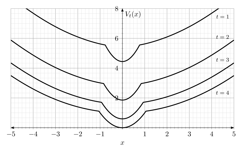
Figure 1: The value function for the remote estimation problem of horizon $T=4$ with state space $\mathds{X}=\mathds{R}$, action space $\mathds{U}=\{0,1\}$, $a=1$, $W_{t}\sim\mathcal{N}(0,1)$, $d(e)=e^{2}$, $\lambda=1$, $q(0)=0$, and $q(1)=0.9$. The kink in the value function corresponds to the point where the optimal action changes. The value functions of the folded MDP are identical to the value functions above when restricted to the domain $\mathds{R}_{\geq 0}$.

To illustrate the above result, consider the case when $\mathds{X}=\mathds{R}$, $\mathds{U}=\{0,1\}$, $a=1$, $W_{t}\sim\mathcal{N}(0,1)$, $d(e)=e^{2}$, $\lambda=1$, $q(0)=0$, $q(1)=0.9$, and $T=4$. We discretize the state space with a uniform grid of width $0.01$ and numerically solve the resulting dynamic program (2)–(4). The value functions across time are shown in Fig. 1. The optimal strategy is of the form

$$g_{t}(e)=\begin{cases}1,&\hbox{if $|e|>k_{t}$}\\ 0,&\hbox{if $|e|\leq k_{t}$}\end{cases}$$

where $k_{1}=0.77$, $k_{2}=0.84$, $k_{3}=0.93$, and $k_{4}=1.05$. Note that, as expected, both the value function and the optimal policy and even and quasi-convex.

VI-A Some comments on the conditions

Note that the result does not depend on (M1). This is for the following reason. Suppose there are two power levels $u_{1},u_{2}\in\mathds{U}$ such that $u_{1}<u_{2}$ but $\lambda(u_{1})\geq\lambda(u_{2})$, then for any $e\in\mathds{X}$, $c(e,u_{1})\geq c(e,u_{2})$. Thus, action $u_{1}$ is dominated by action $u_{2}$ and is, therefore, never optimal and can be eliminated.

All other conditions, (M0), (M2)–(M5) are also necessary as is explained below.

Condition (M2) is necessary. We illustrate that with the following example. Consider an example where $\mathds{X}=\mathbb{Z}$ and $\mathds{U}=\{0,u_{1},u_{2}\}$ such that $u_{1}<u_{2}$ but $q(u_{1})>q(u_{2})$. Then, we can consider an alternative action space $\mathds{U}^{\prime}=\{0,u^{\prime}_{1},u^{\prime}_{2}\}$ where $u^{\prime}_{1}<u^{\prime}_{2}$ and the bijection $\sigma:\mathds{U}\to\mathds{U}^{\prime}$ such that $\sigma(0)=0$, $\sigma(u_{1})=u^{\prime}_{2}$ and $\sigma(u_{2})=u^{\prime}_{1}$. Now consider a remote estimation system with communication cost $\lambda^{\prime}=\lambda\circ\sigma^{-1}$ and success probabilities $q^{\prime}=q\circ\sigma^{-1}$. By construction $q^{\prime}$ satisfies (M0) and (M2). If $d(\cdot)$ and $\varphi(\cdot)$ are chosen to satisfy (M3)–(M5), then by Theorem 4, the optimal strategy $g^{\prime}\colon\mathds{X}\to\mathds{U}^{\prime}$ is even and quasi-convex. In particular, we can pick $\lambda$, $d$ and $\varphi$ such that $g^{\prime}(0)=0$, $g^{\prime}(\pm 1)=u^{\prime}_{1}$ and $g^{\prime}(\pm 2)=u^{\prime}_{2}$. However, this means that with the original labels, the optimal strategy would have been $g=g^{\prime}\circ\sigma^{-1}$, which means $g(0)=0$, $g(\pm 1)=u_{2}$ and $g(\pm 2)=u_{1}$. And hence, the optimal strategy is not quasi-convex.

Conditions (M3) and (M4) are necessary. If they are not satisfied, then it is easy to construct examples where the value function is not even.

Condition (M5) is also necessary. We illustrate that with the following example. Consider an example where $\mathds{X}=\mathbb{Z}$. In particular, let $a=1$ and $\varphi$ have support $\{-1,0,1\}$ where $\varphi(0)=1-2p$ and $\varphi(-1)=\varphi(1)=p$. Suppose $p>1/3$, so that (M5) is not satisfied. Furthermore, suppose $T=2$, $\mathds{U}=\{0,1\}$ and consider the following functions: $\lambda(0)=0$, $\lambda(1)=K$; $q(0)=0$ and $q(1)=1$; and $d(0)=0$, $d(\pm 1)=1$, and for any $e\not\in\{-1,0,1\}$, $d(e)=1+k$, where $k$ is a positive constant. Note that $q(\cdot)$ satisfies (M0) and (M2); $d(\cdot)$ satisfies (M3); and $\varphi(\cdot)$ satisfies (M4) but not (M5). Suppose $K>2(1+k)$, so that action $1$ is not optimal at any time. Thus, $V_{2}(e)=d(e)$ and $V_{1}(0)=2p$ and $V_{1}(\pm 1)=p(1+k)+(1-2p)=pk+1-p$. Now, if $k<(3p-1)/p$, then $V_{1}(-1)<V_{1}(0)>V_{1}(1)$ and hence the value function is not quasi-convex. Hence, condition (M5) is necessary.

VII Conclusion

In this paper we consider a Markov decision process with continuous or discrete state and action spaces and analyze the monotonicity of the optimal solutions. In particular, we identify sufficient conditions under which the value function and the optimal strategy are even and quasi-convex. The proof relies on a folded representation of the Markov decision process and uses stochastic monotonicity and submodularity. We present an example of optimal power allocation in remote estimation and show that the sufficient conditions are easily verified.

Establishing that the value function and optimal strategy are even and quasi-convex has two benefits. First, such structured strategies are easier to implement. Second, the structure of the value function and optimal strategy may be exploited to efficiently solve the dynamic program.

For example, when the action space is discrete, say $|\mathds{U}|=m$, then even and quasi-convex strategy is characterized by $m-1$ thresholds. Such a threshold-based strategy is simpler to implement than an arbitrary strategy. Furthermore, the threshold structure also simplifies the search of the optimal strategy. For discrete state spaces, see the monotone dynamic programming presented in Sec. V-A; for continuous state spaces, see [28], where a simulation based algorithm is presented to compute the optimal thresholds in remote estimation over a packet drop channel.

Even for continuous action spaces, it is easier to search within the class of even and quasi-convex strategies. Typically, some form of approximation is needed to search for an optimal strategy. Two commonly used approximation schemes are discretizing the action space or projecting the policy on to a parametric family of function. If the action state is discretized, then the search methods for discrete action spaces may be used. If the strategy is projected on to a parametric family of function, then the structure may help in reducing the size of the parameter space. For example, when approximating an even and quasi-convex policy as a finite order polynomial, one can restrict attention to polynomials where the coefficients of even powers are positive and the coefficients of odd powers are zero.

In this paper, we assumed that the state space $\mathds{X}$ was a subset of reals. It will be useful to generalize these results to higher dimensions.

Appendix A Proof of Claim 1

We first prove some intermediate results:

Lemma 2

Under (M4) and (M5), for any $x,y\in\mathds{X}_{\geq 0}$, we have that

$$\varphi(y-x)\geq\varphi(y+x)$$

_□

Proof

We consider two cases: $y\geq x$ and $y<x$.

1. If $y\geq x$, then $y+x\geq y-x\geq 0$. Thus, (M5) implies that $\varphi(y+x)\geq\varphi(y-x)$.

2. If $y<x$, then $y+x\geq x-y$. Thus, (M5) implies that $\varphi(y+x)\geq\varphi(x-y)=\varphi(y-x)$, where the last equality follows from (M4).

_■

Some immediate implications of Lemma 2 are the following.

Lemma 3

Under (M4) and (M5), for any $a\in\mathds{X}$ and $x,y\in\mathds{X}_{\geq 0}$, we have that

$$a\big{[}\varphi(y-ax)-\varphi(y+ax)\big{]}\geq 0.$$

_□

Proof

For $a\in\mathds{X}_{\geq 0}$, from Lemma 2 we get that $\varphi(y-ax)\geq\varphi(y+ax)$. For $a\in\mathds{X}_{<0}$, from Lemma 2 we get that $\varphi(y+ax)\geq\varphi(y-ax)$. _■

Lemma 4

Under (M4) and (M5), for any $a,b,x,y\in\mathds{X}_{\geq 0}$, we have that

$$\varphi(y-ax-b)\geq\varphi(y+ax+b)\geq\varphi(y+ax+b+1).$$

_□

Proof

By taking $y=y-b$ and $x=ax$ in Lemma 2, we get

$$\varphi(y-b-ax)\geq\varphi(y-b+ax).$$

Now, by taking $y=y+ax$ and $x=b$ in Lemma 2, we get

$$\varphi(y+ax-b)\geq\varphi(y+ax+b).$$

By combining these two inequalities, we get

$$\varphi(y-ax-b)\geq\varphi(y+ax+b).$$

The last inequality in the result follows from (M5). _■

Lemma 5

Under (M4) and (M5), for $a\in\mathbb{Z}$ and $x,y\in\mathbb{Z}_{\geq 0}$,

$$\Phi(y+ax)+\Phi(y-ax)\geq\Phi(y+ax+a)+\Phi(y-ax-a),$$

where $\Phi$ is the cdf (cumulative distribution function) of $\varphi$. _□

Proof

The statement holds trivially for $a=0$. Furthermore, the statement does not depend on the sign of $a$. So, without loss of generality, we assume that $a>0$.

Now consider the following series of inequalities (which follow from Lemma 4)

$$\varphi(y-ax) \geq\varphi(y+ax+1),$$

$$\varphi(y-ax-1) \geq\varphi(y+ax+2),$$

$$\cdots \geq\cdots$$

$$\varphi(y-ax-a+1) \geq\varphi(y+ax+a).$$

Adding these inequalities, we get

$$\Phi(y-ax)-\Phi(y-ax-a)\geq\Phi(y+ax+a)-\Phi(y+ax),$$

which proves the result. _■

Proof of Claim 1

First, let’s assume that $\mathds{X}=\mathds{R}$. We prove each part separately.

1. Fix $u\in[0,u_{\max}]$. $c(\cdot,u)$ is even because $d(\cdot)$ is even (from (M3)). $c(\cdot,u)$ is quasi-convex because $1-q(u)\geq 0$ (from (M0)) and $d(\cdot)$ is quasi-convex (from (M3)).

2. Consider $e_{1},e_{2}\in\mathds{R}_{\geq 0}$ and $u_{1},u_{2}\in[0,u_{\max}]$ such that $e_{1}\geq e_{2}$ and $u_{1}\geq u_{2}$. The per-step cost is submodular on $\mathds{R}_{\geq 0}\times[0,u_{\max}]$ because

   $$c(e_{1},u_{2})-c(e_{2},u_{2}) =(1-q(u_{2}))(d(e_{1})-d(e_{2}))$$

   $$\stackrel{{\scriptstyle(a)}}{{\geq}}(1-q(u_{1}))(d(e_{1})-d(e_{2}))$$

   $$=c(e_{1},u_{1})-c(e_{2},u_{1}),$$

   where $(a)$ is true because $d(e_{1})-d(e_{2})\geq 0$ (from (M3)) and $1-q(u_{2})\geq 1-q(u_{1})\geq 0$ (from (M0) and (M2)).

3. Fix $u\in[0,u_{\max}]$ and consider $e,e_{+}\in\mathds{R}$. Then, $p(u)$ is even because

   $$p(-e_{+}|{-e};u) =q(u)\varphi(e_{+})+(1-q(u))\varphi(-e_{+}+ae)$$

   $$\stackrel{{\scriptstyle(b)}}{{=}}q(u)\varphi(e_{+})+(1-q(u))\varphi(e_{+}-ae)$$

   $$=p(e_{+}|e;u),$$

   where $(b)$ is true because $\varphi$ is even (from (M4)).

4. First note that

   $$\hskip-10.00002ptS(y|x;u)=1-\int_{-\infty}^{y}\big{[}p(z|x;u)+p(-z|x;u)\big{]}dz$$

   $$=1-\int_{-\infty}^{y}q(u)\big{[}\varphi(z)+\varphi(-z)\big{]}dz$$

   $$\quad-\int_{-\infty}^{y}(1-q(u))\big{[}\varphi(z-ax)+\varphi(-z-ax)]dz$$

   $$\stackrel{{\scriptstyle(c)}}{{=}}1-2q(u)\Phi(y)$$

   $$\quad-(1-q(u))\big{[}\Phi(y-ax)+\Phi(y+ax)\big{]}$$

   where $\Phi$ is the cumulative distribution of $\varphi$ and $(c)$ uses the fact that $\varphi$ is even (condition (M4)).

   Let $S_{x}(y|x;u)$ denote $\partial S/\partial x$. Then

   $$S_{x}(y|x;u)=(1-q(u))a\big{[}\varphi(y-ax)-\varphi(y+ax)\big{]}.$$

   From (M0) and Lemma 3, we get that $S_{x}(y|x;u)\geq 0$ for any $x,y\in\mathds{R}_{\geq 0}$ and $u\in[0,u_{\max}]$. Thus, $S(y|x;u)$ is increasing in $x$.

   Furthermore, from (M2) $S_{x}(y|x;u)$ is decreasing in $u$. Thus, $S(y|x;u)$ is submodular in $(x,u)$ on $\mathds{R}_{\geq 0}\times[0,u_{\max}]$.

Now, let’s assume that $\mathds{X}=\mathbb{Z}$. The proof of the first three parts remains the same. Now, in part 4), it is still the case that

$$S(y|x;u)=1-2q(u)\Phi(y)\\ -(1-q(u))\big{[}\Phi(y-ax)+\Phi(y+ax)\big{]}$$

However, since $\mathds{X}$ is discrete, we cannot take the partial derivative with respect to $x$. Nonetheless, following the same intuition, for any $x,y\in\mathbb{Z}_{\geq 0}$, consider

$$S(y|x+1;u)-S(y|x;u)=(1-q(u))\big{[}\Phi(y+ax)\\ {}-\Phi(y+ax+a)+\Phi(y-ax)-\Phi(y-ax-a)\big{]}$$ (13)

Now, by Lemma 5, the term in the square bracket is positive, and hence $S(y|x;u)$ is increasing in $x$. Moreover, since $(1-q(u))$ is decreasing in $u$, so is $S(y|x+1;u)-S(x|x;u)$. Hence, $S(y|x;u)$ is submodular in $\mathds{Z}_{\geq 0}\times[0,u_{\max}]$.

References

• [1] C. Derman, Mathematical optimization techniques.   University of California Press, Apr. 1963, ch. On optimal replacement rules when changes of state are Markovian, pp. 201–209.
• [2] P. Kolesar, “Minimum cost replacement under Markovian deterioration,” Management Science, vol. 12, no. 9, pp. 694–706, May 1966.
• [3] H. M. Taylor, “Evaluating a call option and optimal timing strategy in the stock market,” Management Science, vol. 14, no. 1, pp. 111–120, Sep. 1967.
• [4] R. C. Merton, “Theory of rational option pricing,” The Bell Journal of Economics and Management Science, vol. 4, no. 1, pp. 141–183, 1973.
• [5] M. J. Sobel, Mathematical methods in queueing theory.   Springer, 1974, ch. Optimal operation of queues, pp. 231–261.
• [6] S. Stidham Jr and R. R. Weber, “Monotonic and insensitive optimal policies for control of queues with undiscounted costs,” Operations Research, vol. 37, no. 4, pp. 611–625, Jul.–Aug. 1989.
• [7] R. F. Serfozo, Stochastic Systems: Modeling, Identification and Optimization, II.   Berlin, Heidelberg: Springer, 1976, ch. Monotone optimal policies for Markov decision processes, pp. 202–215.
• [8] M. Puterman, Markov decision processes: Discrete Stochastic Dynamic Programming.   John Wiley and Sons, 1994.
• [9] C. C. White, “Monotone control laws for noisy, countable-state Markov chains,” European Journal of Operational Research, vol. 5, no. 2, pp. 124–132, 1980.
• [10] S. M. Ross, Introduction to Stochastic Dynamic Programming.   Orlando, FL, USA: Academic Press, Inc., 1983.
• [11] D. P. Heyman and M. J. Sobel, Stochastic Models in Operations Research.   New York, USA: McGraw Hill, 1984.
• [12] N. L. Stokey and R. E. Lucas, Jr, Recursive methods in economic dynamics.   Harvard University Press, 1989.
• [13] D. M. Topkis, “Minimizing a submodular function on a lattice,” Oper. Res., vol. 26, no. 2, pp. 305–321, Mar.–Apr. 1978.
• [14] ——, Supermodularity and Complementarity, D. M. Kreps and T. J. Sargent, Eds.   Princeton University Press, 1998.
• [15] K. Papadaki and W. B. Powell, “Monotonicity in multidimensional Markov decision processes for the batch dispatch problem,” Operations research letters, vol. 35, no. 2, pp. 267–272, Mar. 2007.
• [16] J. E. Smith and K. F. McCardle, “Structural properties of stochastic dynamic programs,” Operations Research, vol. 50, no. 5, pp. 796–809, Sep.–Oct. 2002.
• [17] O. C. Imer and T. Basar, “Optimal estimation with limited measurements,” in Joint 44th IEEE Conference on Decision and Control and European Control Conference, Dec. 2005, pp. 1029–1034.
• [18] G. M. Lipsa and N. C. Martins, “Remote state estimation with communication costs for first-order LTI systems,” IEEE Trans. Autom. Control, vol. 56, no. 9, pp. 2013–2025, Sep. 2011.
• [19] A. Molin and S. Hirche, “An iterative algorithm for optimal event-triggered estimation,” in 4th IFAC Conference on Analysis and Design of Hybrid Systems, Jun. 2012, pp. 64–69.
• [20] A. Nayyar, T. Basar, D. Teneketzis, and V. V. Veeravalli, “Optimal strategies for communication and remote estimation with an energy harvesting sensor,” IEEE Trans. Autom. Control, vol. 58, no. 9, pp. 2246–2260, Sep. 2013.
• [21] J. Chakravorty and A. Mahajan, “Fundamental limits of remote estimation of Markov processes under communication constraints,” IEEE Trans. Autom. Control, vol. 62, no. 3, pp. 1109–1124, Mar. 2017.
• [22] ——, “Remote-state estimation with packet drop,” in IFAC Workshop on Dist. Estim. Control in Networked Sys., Sep. 2016, pp. 7–12.
• [23] ——, “Structure of optimal strategies for remote estimation over Gilbert-Elliott channel with feedback,” arXiv: 1701.05943, Jan. 2017.
• [24] Y. Xu and J. P. Hespanha, “Optimal communication logics in networked control systems,” in 43rd IEEE Conference on Decision and Control, vol. 4, Dec. 2004, pp. 3527–3532.
• [25] O. Hernández-Lerma and J. Lasserre, Discrete-Time Markov Control Processes.   Springer-Verlag, 1996.
• [26] L. Shi and L. Xie, “Optimal sensor power scheduling for state estimation of Gauss-Markov systems over a packet-dropping network,” IEEE Trans. Signal Process., vol. 60, no. 5, pp. 2701–2705, May 2012.
• [27] X. Ren, J. Wu, K. H. Johansson, G. Shi, and L. Shi, “Infinite Horizon Optimal Transmission Power Control for Remote State Estimation over Fading Channels,” arXiv: 1604.08680, Apr. 2016.
• [28] J. Chakravorty, J. Subramanian, and A. Mahajan, “Stochastic approximation based methods for computing the optimal thresholds in remote-state estimation with packet drops,” in American Control Conference, May 2017.