An analysis of budgeted parallel search on conditional Galton-Watson trees

An analysis of budgeted parallel search on conditional Galton-Watson trees

Abstract

Recently Avis and Jordan have demonstrated the efficiency of a simple technique called budgeting for the parallelization of a number of tree search algorithms. The idea is to limit the amount of work that a processor performs before it terminates its search and returns any unexplored nodes to a master process. This limit is set by a critical budget parameter which determines the overhead of the process. In this paper we study the behaviour of the budget parameter on conditional Galton-Watson trees obtaining asymptotically tight bounds on this overhead. We present empirical results to show that this bound is surprisingly accurate in practice.

Keywords: Parallel tree search, random Galton-Watson tree, probabilistic analysis of algorithms, branching process.

1 Introduction

The majority of algorithms have been designed, analyzed and implemented to run on single core processors. While multicore hardware is now ubiquitous these algorithms profit little, if any, from the additional processing power. On the other hand, the study of parallel algorithms also has a long history. Issues involved are complex and include architecture design, communication, data sharing, interrupts, deadlocks, load balancing, and the distinction between shared memory and distributed computing. For a comprehensive reference, see Mattson (2004). This complexity presents serious challenges to developing theoretical analyses to explain successful empirical results. Indeed many recent highly publicized computational success stories, such as Computer Go, Machine Learning and Deep Learning for AI, make massive use of parallel computation but have little or no theoretical foundation for the underlying algorithms.

In a recent paper, McCreesh and Prosser (2015) attempt to fill this gap in the context of parallel branch and bound algorithms for the maximum clique problem. They show that the interaction of the search order and the most likely location of solutions is often the dominant consideration in load balancing for these types of problems. This leads to a new work-splitting technique which gives good scalability. In their conclusions they recall the following prescient remark of Hooker (1995):

Based on one’s insight into an algorithm, for instance, one might expect good performance to depend on a certain characteristic. How to find out? Design a controlled experiment that checks how the presence or absence of this characteristic affects performance. Even better, build an explanatory mathematical model that captures the insight, as is done routinely in other empirical sciences, and deduce from it precise consequences that can be put to the test.

The purpose of this paper is to make a modest additional contribution along these lines by giving a theoretical analysis of the overhead produced by a simple and effective scaleable parallelization technique, described by Avis and Jordan (2015, 2016), that is applicable to a certain class of tree search algorithms. This class includes reverse search which has been used for a large number of combinatorial and geometric enumeration problems. Trees in this class must be definable by an oracle which, given any node in the tree, gives the children of that node (if any) in an arbitrary but fixed order. Traversals of trees in this class can be performed in parallel by assigning independent subtrees to different processors. When the underlying tree is unbalanced, the main problem again becomes one of load balancing. The tree traversal problem differs significantly from branch and bound, where the goal is to explore as little of the tree as possible until a desired node is found. The bounding step removes subtrees from consideration and this step depends critically on what has already been discovered. Hence the order of traversal is crucial and the number of nodes evaluated varies dramatically depending on this order, as reported by McCreesh and Prosser (2015). Sharing of information is critical to the success of parallelization in branch and bound. These issues do not occur when the entire tree must be traversed, hence simpler parallelization techniques are possible.

Avis and Jordan approach the load balancing problem by using a simple technique called budgeting. A search of a subtree of the original tree terminates after a given number of nodes, called the budget, have been generated and returns all unexplored nodes to a master process which stores them on a job list. In a multiprocessor setting, the master process assigns nodes from the job list to available processors, called workers, that proceed in parallel, repopulating the list whenever their budget is reached. In their 2015 paper they apply this technique to parallelize lrs, a reverse search based code for the vertex/facet enumeration problem for convex polyhedra. Experimental results showed near linear speedups when using up to several hundred processors. In the second paper the authors describe a generic common wrapper that can be used with a wide variety of legacy codes. They gave applications to other reverse search codes and, more recently, to satisfiability testers, again obtaining substantial speedups. The resulting software, called mts , is freely available. Budgeting may be seen as a very simple form of job stealing, as described by Blumofe and Leiserson (1999). However in job stealing individual workers maintain their own job lists and poll each other as necessary to obtain additional work, requiring communications between workers, interrupt handling, deadlock avoidance and so on.

Budgeting has several very practical advantages. Firstly it does not require communication between workers and they do not need to process interrupts. This means that parallelism does not have to be added to the existing legacy code. Secondly large subtrees are automatically broken up, since they exceed the budget, whereas small subtrees are not, since they do not. Thirdly the master can dynamically control the size of the job list by varying the size of the budget when assigning work. Finally it is easy to checkpoint the process since all workers return to the master regularly due to the budget restriction. It is simply a matter of waiting for all workers to return and then outputting the remaining job list. On the other hand budgeting introduces two competing forms of overhead. One is the cost of restarting jobs on the master’s list, which is directly proportional to the total size of the list. The other is the cost of idle workers if the list becomes empty. It is therefore very important to determine how the budget parameter affects the size of the job list.

The goal of this paper is to analyze the budgeting method when it is applied to critical Galton-Watson trees. These trees provide a challenge to efficient parallel search since they are very unbalanced: it is well-known, see, e.g., Flajolet and Odlyzko (1982), that the height of such trees is of the order or the square root of their size. For this class of trees we study the critical budget parameter and how it determines the size and evolution of the job list. In Section 2 we formally introduce budgeting and give an explicit example of how it can be implemented in a depth first search setting. Next, in Section 3 we introduce Galton-Watson trees and observe that they include quite a large number of other classes of random trees. We then state our main result, a tight estimate on the overhead produced by budgeting for traversing trees in our family. In Section 4 we describe a random walk which is closely related to the evolution of the list of unexplored nodes produced by budgeting. This is followed in Section 5 by a proof of our main result. Finally in Section 6 we make use of the mts framework to empirically test our estimates on a sample of large Galton-Watson trees. We also give a discussion of how our main result can be used in a multiprocessor setting in order to choose an efficient budget parameter.

2 Budgeted tree search

We are given a tree $T$ by its root, an upper bound $\Delta$ on the number of children of any node, and an adjacency oracle $Adj(v,j)$. The adjacency oracle takes a tree node $v$ and an index $j\in\{0,1,2,...,\Delta-1\}$. For each value of $j$ in its range, $Adj(v,j)$ either returns $null$ or gives a child of $v$. Each child is given exactly once. Our goal is to visit all of the nodes in $T$. For concreteness in this section we will describe depth first search (DFS) although the budgeting technique can be applied to breadth first search or other search strategies.

A budgeted DFS is initiated from tree node $start\_vertex$, initially set to be the root, and proceeds in a depth first fashion outputting each node as it is generated. We use two stacks, $stack\_v$ to store vertices and $stack\_j$ to store indices. We also specify an integer budget parameter $b\geq 1$ which causes the tree search to be terminated when $b$ nodes have been generated. At this point the most recently generated vertex $v$ and all of the unexplored siblings along the return path from $v$ to $start\_vertex$ are returned with the flag unexplored=true. All previously generated nodes were output with the flag unexplored=false. The pseudo-code is shown as Algorithm 1. Note that that $start\_vertex$ is not output so this should be done in the calling program. We exploit this property later.

1:procedure bdfs($start\_vertex$, $\Delta$, $Adj$, $b$ )

2:     $j\leftarrow 0~{}~{}~{}v\leftarrow start\_vertex~{}~{}~{}count\leftarrow 0~{}~{}~{}depth\leftarrow 0$

3:     repeat

4:         $unexplored\leftarrow false$

5:         while $j<\Delta$ and $unexplored=false$  do

6:              $j\leftarrow j+1$

7:              $push(stack\_v,v)$

8:              $push(stack\_j,j)$

9:              $v\leftarrow Adj(v,j)~{}~{}~{}~{}~{}$

10:              $depth\leftarrow depth+1~{}~{}~{}~{}count\leftarrow count+1$

11:              if $count\geq b$ then $\triangleright$ budget is exhausted

12:                  $unexplored\leftarrow true$

13:              end if

14:              output $(v,unexplored)$

15:              if $count<b$ then $\triangleright$ continue down tree

16:                  $j\leftarrow 0$

17:              end if

18:         end while

19:         if $depth>0$ then $\triangleright$ backtrack step

20:              $v\leftarrow pop(stack\_v)$

21:              $j\leftarrow pop(stack\_j)$

22:              $depth\leftarrow depth-1$

23:         end if

24:     until $depth=0$ and $j=\Delta$

25:end procedure

Algorithm 1 Budgeted depth first search

Consider the tree in Figure 1 which has 25 nodes, $\Delta=5$ and is rooted at vertex 0. For convenience the nodes are numbered 0,1,…,24 in depth first search order but this is in no way essential. If we set the parameter $b$ to be 25 or greater, all nodes are output in this order with unexplored=false. Suppose we set $b=13$. Firstly nodes 1,…,12 are output in order with unexplored=false. Then nodes 13,15,16,18,22 are output with unexplored=true. On the other hand, if we set $b=8$ then nodes 1,2,…,7 are output with unexplored=false and nodes 8,9,10,11,15,16,18,22 are output with unexplored=true.

Figure 1: Tree rooted at vertex 0 with 25 nodes and $\Delta=6$

We will store the unexplored nodes in a list $L$ which, for DFS, would be implemented as a stack. To complete the DFS of the tree we search the subtrees rooted by nodes in $L$ using Algorithm 1 repeatedly. Note that each vertex in $L$ now becomes a $start\_vertex$ and if a budget constraint $b$ is applied additional nodes may be added to $L$. If $L$ is empty when Algorithm 1 terminates the tree has been completely output. Since the root nodes are not output we will obtain a duplicate free list of all the nodes of the tree by concatenating outputs. Note that if the order of output is not important, the subtrees rooted by nodes in $L$ can be explored in any order and in parallel. Furthermore, if $b=1$ then all nodes in $T$ will be returned to $L$. Alternatively, if $b>|T|$ then $L$ remains empty as the tree is explored with a single call to Algorithm 1.

A successful parallelization of Algorithm 1 depends on controlling the job list $L$. On one hand, if the budget parameter $b$ is too small, then $L$ tends to become large causing considerable overhead in restart costs. If $b$ is too large, then $L$ becomes smaller, reducing overhead, but may become empty before the entire tree has been searched. This causes processors to become idle and reduces the speedup that can be obtained. We are interested in how $L$ evolves over time.

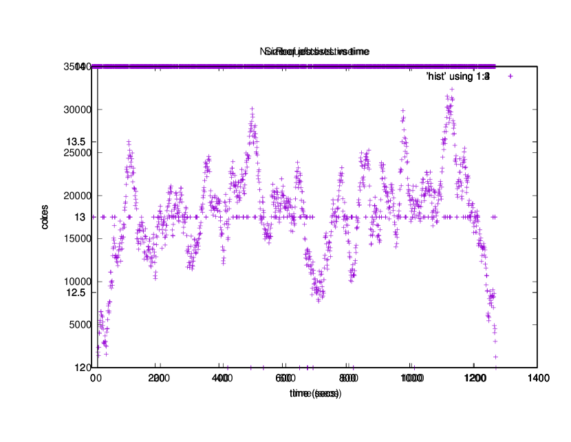
(a) $b=50,~{}R_{n}=52,454,166$

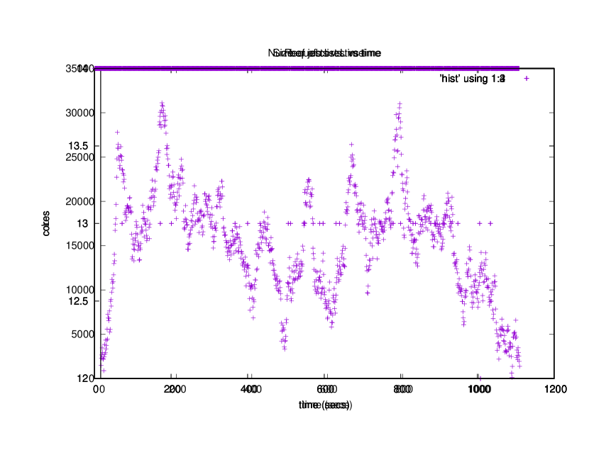
(b) $b=500,~{}R_{n}=17,384,235$

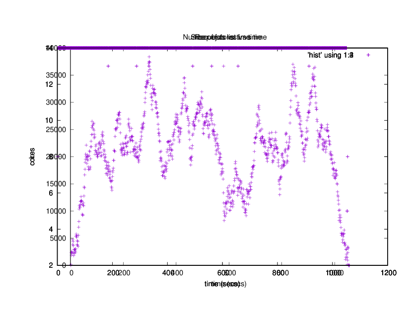
(c) $b=5000,~{}R_{n}=5,584,327$

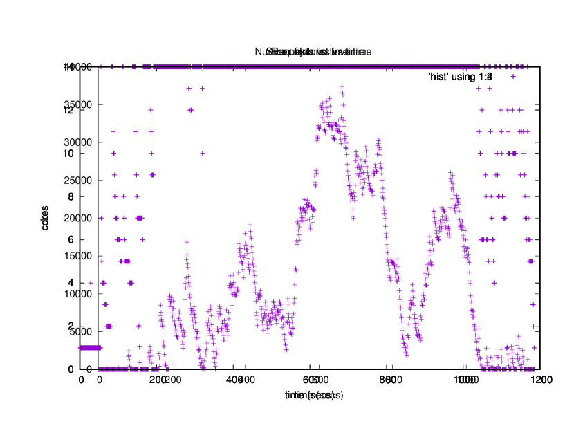
(d) $b=500,000,~{}R_{n}=572,507$

Figure 2: Evolution of the job list for $T_{10}$: budget=$b$, total restarts=$R_{n}$, mai20, 16 cores

Let $L_{b}$ be the job list generated by repeatedly applying Algorithm 1 to a tree $T$ for a given budget $b$ and let $R_{n}$ denote the total number of nodes added to the list during a complete search of $T$. We can observe the size of $L_{b}$ each time Algorithm 1 is called. For example, again referring to Figure 1, Algorithm 1 is called a total of 6 times if we keep $b=13$ throughout. $|L_{13}|=5$ and the size of $L_{13}$ is respectively 0,4,3,2,1,0 for these 6 times.

For a larger example consider Figure 2. This is based on visiting all the nodes of the tree $T_{10}$ which has $\Delta=10$ and 264,933,315 nodes. Its construction is described in detail in Section 6. The plots were obtained by running Algorithm 1 in parallel on 16 cores using mts version 0.1 and different budget sizes $b$.

The first thing to observe is that, as expected, the number $R_{n}$ of jobs returned to $L$ is inversely proportional to $b$. By comparing the results for $b=50,5000,500000$ we see that as the budget scales up by a factor of 100, the size of $R_{n}$ scales down by roughly a factor of 10, the square root of the scale factor. In the following sections we show that this is typical behaviour for Galton-Watson trees, of which $T_{10}$ is a sample.

For $b=50$ and $b=500$ we have the desired behaviour for $L$: it quickly reaches a reasonable size (compared to the total tree size) and remains non-empty until the end of the run, implying all processors are busy. For $b=5,000$ the job list comes dangerously close to being empty before the run ends and for the extreme case $b=500,000$ it is empty for several time intervals. All things being equal a small budget would seem optimum. However in practical applications, such as vertex enumeration, the startup cost for a job taken from $L$ can be very significant. A budget small enough to keep a non-empty job list yet large enough to prevent too many restarts leads to optimum performance.

Before proceeding we note two important points. Firstly the total size of the job list is independent of the number of workers assigned. Indeed a single worker repeatedly executing Algorithm 1 produces the same number of jobs as a thousand workers in parallel. Secondly, if the job list stays well populated for the duration of the run then workers are never idle. If the jobs on the list are independent, as they are in a Galton-Watson tree, then each worker behaves in the same way in probability. It is therefore sufficient to study the behaviour of a single worker applying Algorithm 1 repeatedly until the job list is empty.

3 The probabilistic model and our main result

A Galton-Watson (or Galton-Watson-Bienaymé) tree (see Athreya and Ney, 1972) is a rooted random ordered tree. Each node independently generates a random number of children drawn from a fixed offspring distribution $\xi$. The distribution of $\xi$ defines the distribution of $T$, a random Galton-Watson tree. In what follows, we are mainly interested in critical Galton-Watson trees, i.e., those having ${{E}}\{\xi=1\}$, and ${{P}}\{\xi=1\}<1$. In addition, we assume that the variance of $\xi$ is finite (and hence, nonzero).

Moon (1970) and Meir and Moon (1978) defined the simply generated trees as ordered labelled trees of size $n$ that are all equally likely given a certain pattern of labeling for each node of a given degree. The most important examples include the Catalan trees (equiprobable binary trees), the equiprobable $k$-ary trees, equiprobable unary-binary trees (ordered trees with up to two children), random Motzkin trees, random planted plane trees (equiprobable ordered trees of unlimited degrees) and Cayley trees (equiprobable unordered rooted trees). It turns out that all these trees can be represented as critical Galton-Watson trees conditional on their size, $n$, a fact first pointed out by Kennedy (1975), and further developed by Kolchin (1980, 1986) and others. So, let $T_{n}$ be a Galton-Watson tree conditional on its size being $n$. For example, when $\xi$ is $0$ or $2$ with probability $1/4$, and $1$ with probability $1/2$, we obtain the uniform binary (Catalan) tree. Uniformly random full binary trees are obtained by setting ${{P}}\{\xi=0\}={{P}}\{\xi=2\}=1/2$. A uniformly random $k$-ary tree has its offspring distributed as a binomial $(k,1/k)$ random variable. A uniform planted plane tree is obtained for the geometric law ${{P}}\{\xi=i\}=1/2^{i+1}$, $i\geq 0$. When $\xi$ is Poisson of parameter $1$, one obtains (the shape of) a random rooted labeled (or Cayley) tree. For $\xi$ uniform on $\{0,1,2,\ldots,k\}$, $T_{n}$ is like a uniform ordered tree with maximal degree of $k$. All such trees can be dealt with at once in the Galton-Watson framework.

Recall that $R_{n}$ is the number of restarts generated when Algorithm 1 is used repeatedly to explore a tree $T$ with $n$ nodes using a budget $b$. Our main result is:

Theorem 1. If $T_{n}$ is a Galton-Watson tree of size $n$ determined by $\xi$, where ${{E}}\{\xi\}=1$ and $0<{{V}}\{\xi\}\buildrel{\rm def}\over{=}\sigma^{2}<\infty$, then

$${R_{n}\over n}\to{1\over\mu_{b}}$$

in probability as $n\to\infty$, where

$$\mu_{b}\buildrel{\rm def}\over{=}{{E}}\{\min(|T|,b)\},$$

and $T$ is an unconditional Galton-Watson tree for the same $\xi$. In addition, as $b\to\infty$,

$$\mu_{b}\sim\sqrt{8b\over\pi\sigma^{2}}.$$

4 4

Preliminary results: the random walk view

Let $\xi$ be a random variable representing the number of children of the root in a critical Galton-Watson tree: ${{E}}\{\xi\}=1$, ${{P}}\{\xi=0\}>0$. Set $X=\xi-1$, and let $X_{1},X_{2},\ldots$ be a sequence of i.i.d. random variables distributed as $X$. Define the partial sums $Q(0)=1$, $Q(t)=1+\sum_{i=1}^{t}X_{i}$. There is a well-known depth first or preorder construction of a random Galton-Watson tree which lends itself well to the study of all properties of randomly selected nodes (see, e.g., Le Gall, 1989, or Aldous, 1991). Nodes in an ordered tree can be encoded with a vector of child numbers. The root corresponds to the empty vector. Its children have encodings $1,2,\ldots,\xi$. More generally, the $i-th$ child of a node with label $j$ is encoded $(j,i)$. A preorder listing of the nodes is nothing but a lexicographic listing of the node vectors.

We can traverse a random Galton-Watson tree by visiting nodes in preorder, starting at the root. To do so, a list $V$ of nodes to be visited is kept, which is initially of size one ($V$ just contains the root). When node $u$ is visited, we consider $\xi_{u}$, the number of children of $u$, and remove $u$ from $V$. Thus, $V$ increases by $\xi_{u}-1$. The next node in lexicographic order is taken from $V$, and the process continues until $V$ is empty.

We denote by $N$ the size of a random Galton-Watson tree. The size of $V$ after $t$ nodes have been processed is precisely the $Q$ process introduced above, $Q(t)$. Thus, $Q(0)=1$, and

$$Q(t)=1+X_{1}+\cdots+X_{t},$$

where $X_{t}=\xi_{t}-1$, and indexing of the nodes is by their lexicographic rank. An example of the $Q$ process derived from a tree is shown in Figure 3. The path in the grid from vertex (0,1) to vertex (9,0) is derived from a preorder traversal of the tree to the right. Except for vertex (9,0), each vertex of the path is of the form $(x,Q(x))$ where $x$ is the tree node to be explored next and $Q(x)$ is the number of unexplored tree nodes we have discovered so far. We start at (0,1) as $V$ contains only the root 0 and so $V$ has size $Q(0)=1$. Since the root has two children the list of unexplored nodes becomes $\{1,8\}$ which has length 2 so we move to vertex (1,2) in the grid. Tree node 1 has 3 children so the list becomes $\{2,3,7,8\}$ with length 4, we move to (2,4) and so on. Finally we explore node 8 which has no children, the unexplored list is empty and we terminate the Q process.

We have the identity

$$[N=n]=[Q(1)>0,Q(2)>0,\ldots,Q(n-1)>0,Q(n)=0].$$

The standard circular symmetry argument for random walks (see, e.g., Dwass, 1968) shows that

$$\halign to=0.0pt{\hfil$\@lign\displaystyle{#}$&$\@lign\displaystyle{{}#}$\hfil&\llap{$\@lign#$}\cr{P}\left\{ N = n \right\} &= {P}\left\{ Q(0) = 1 , Q(1) > 0 , Q(2) > 0, \ldots, Q(n-1) > 0, Q(n) = 0 \right\} \cr&= {1 \over n} {P}\left\{ Q(n) = 0 \right\} \cr&= {1 \over n} {P}\left\{ X_{1} + \cdots+ X_{n} = -1 \right\}. \cr}$$

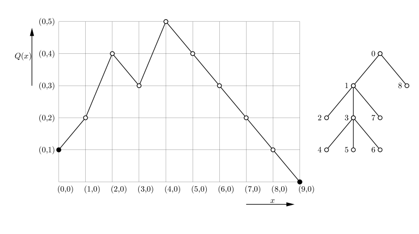
Figure 3: The Q-process derived from a tree

The asymptotics for this probability distribution are well-known, and will be given below. Let $0<\sigma^{2}\buildrel{\rm def}\over{=}{{V}}\{\xi\}>0$ (which implies ${{P}}\{\xi=1\}<1$), and let the span $d$ be the greatest common divisor of all $i>0$ for which ${{P}}\{\xi=i\}>0$. A Galton-Watson tree with span $d$ can only have sizes that are $1~{}\hbox{\rm mod}~{}d$. From Petrov (1975, p. 197) or Kolchin (1986, p. 16, p. 105), we recall that

$$\lim_{n\to\infty}\sup_{k=1~{}\hbox{\rm mod}~{}d}\left|\sigma\sqrt{n}\,{{P}}\left\{X_{1}+\cdots+X_{n}=k\right\}-{d\over\sqrt{2\pi}}e^{-{k^{2}\over 2\sigma^{2}n}}\right|=0,$$

while, clearly, ${{P}}\left\{X_{1}+\cdots+X_{n}=k\right\}=0$ if $k\not=1~{}\hbox{\rm mod}~{}d$. Thus, along $n\in{\cal N}$,

$${{P}}\left\{N=n\right\}\sim{d\over\sigma\sqrt{2\pi}n^{3/2}},$$

and, as $n\to\infty$,

$${{P}}\left\{N\geq n\right\}\sim\sqrt{2\over\pi n\sigma^{2}}.$$

Lemma 1. Under the conditions of Theorem 1, as $b\to\infty$,

$${{E}}\{\min(N,b)\}\sim\sqrt{8b\over\pi\sigma^{2}}.$$

Proof. We have

$$\halign to=0.0pt{\hfil$\@lign\displaystyle{#}$&$\@lign\displaystyle{{}#}$\hfil&\llap{$\@lign#$}\cr{E}\{ \min(N,b) \} &= \sum_{t=1}^{\infty}t {P}\{ \min(N,b) = t \} \cr&= \sum_{t=1}^{b} t {P}\{ N = t \} + b {P}\{ N >b \} \cr&= \sum_{t=1}^{b} {P}\{ X_{1}+\cdots+X_{t} = -1 \} + b {P}\{ N >b \} \cr&= \sum_{t\leq b: t \in{\cal N}} {d+o(1) \over\sigma\sqrt{2 \pi t }} + (1+o(1)) \sqrt{ 2b \over\pi\sigma^{2}} \cr&\sim\int_{1}^{b} {1 \over\sigma\sqrt{2 \pi t}} \,dt + \sqrt{ 2b \over\pi\sigma^{2}} \cr&\sim\sqrt{ 8b \over\pi\sigma^{2}}. ~{}{\vbox{\vbox{\hrule height=0.4pt\hbox{\vrule width=0.4pt,height=7.0pt\kern 7.0pt\vrule width=0.4pt}\hrule height=0.4pt}}}\cr}$$

Consider the $Q$-process conditional on visiting $(x,y)$, with $0<x<n$ and $y>0$. Define

$$S(x,y)=\min\{t>x:Q(t)=Q(x)-1~{}|~{}Q(x)=y\}-x,$$

where we recall that $Q(t)=1+X_{1}+\cdots+X_{t}$. In other words, $S(x,y)$ is the size of the subtree of node $x$ in depth first search order given that $Q(x)=y$. Referring back to the example in Figure 3 we see that $S(0,1)=9,~{}S(1,2)=7,~{}S(2,4)=1,~{}S(3,3)=4,~{}S(4,5)=1,~{}S(5,4)=1,~{}S(6,3)=1,~{}S(7,2)=1,~{}S(8,1)=1.$

Note that $S(x,y)=1~{}\hbox{\rm mod}~{}d$. In addition, since $Q(0)=1$, we must have $t+Q(t)=1~{}\hbox{\rm mod}~{}d$, so that the only values $(x,y)$ of interest to us have $x+y=1~{}\hbox{\rm mod}~{}d$. We consider two positive constants $a$, $c$, with $a<1/2,c<1$, and let ${\cal S}(a,c)$ denote the collection of all random variables $S(x,y)$ with $an\leq x\leq(1-a)n$, $c\sqrt{n}\leq y\leq(1/c)\sqrt{n}$. Lemma 2 below shows that within ${\cal S}(a,c)$, all random variables are close to $N$, the size of an unconditional Galton-Watson tree. This is an explicit version of a well-known theorem due to Aldous (1991) (see also Janson (2012)), which states that if $T^{*}_{n}$ is the subtree of a uniform random node of $T_{n}$, then $T^{*}_{n}$ tends in distribution to an unconditional Galton-Watson tree $T$ as $n\to\infty$.

Lemma 2. For any fixed $0<a<1/2$, $0<c<1$ and integer $b>0$,

$$\lim_{n\to\infty}\sup_{1\leq i\leq b;i=1~{}\hbox{\rm mod}~{}d}\,\sup_{(x,y):\left\{\,\vbox{\halign{$#\hfil$&\quad#\hfil\cr S(x,y)\in{\cal S}(a,c)&\cr x+y=1~{}\hbox{\rm mod}~{}d&\cr}}\right.}\left|{{{P}}\{S(x,y)=i\}\over{{P}}\{N=i\}}-1\right|=0.$$

Furthermore,

$$\lim_{n\to\infty}\sup_{(x,y):\left\{\,\vbox{\halign{$#\hfil$&\quad#\hfil\cr S(x,y)\in{\cal S}(a,c)&\cr x+y=1~{}\hbox{\rm mod}~{}d&\cr}}\right.}\left|{{E}}\{\min(b,S(x,y))\}-{{E}}\{\min(b,N)\}\right|=0.$$

Proof. The last part follows from the first one, so we only consider ${{P}}\{S(x,y)=i\}$ for $1\leq i\leq b$, $i=1~{}\hbox{\rm mod}~{}d$. We have, for $x+y=1~{}\hbox{\rm mod}~{}d$, $n=1~{}\hbox{\rm mod}~{}d$,

$$\halign to=0.0pt{\hfil$\@lign\displaystyle{#}$&$\@lign\displaystyle{{}#}$\hfil&\llap{$\@lign#$}\cr{P}&\{ Q(x)=y, Q(t) > 0 ~{}\hbox{\rm for all}~{}x < t < n, Q(n)=0 \} \cr&= {P}\{ Q(x) = y \} \times{1 \over n-x} {P}\{ X_{1} + \cdots+ X_{n-x} = -y \} \cr&= {P}\{ Q(x) = y \} \times{d+o(1) \over(n-x) \sqrt{2 \pi(n-x) \sigma^{2}}} \exp\left( - {y^{2} \over 2(n-x)\sigma^{2}} \right). \cr}$$

Also,

$$\halign to=0.0pt{\hfil$\@lign\displaystyle{#}$&$\@lign\displaystyle{{}#}$\hfil&\llap{$\@lign#$}\cr{P}&\{ Q(x)=y, S(x,y)=i , Q(t) > 0 ~{}\hbox{\rm for all}~{}x+i < t < n, Q(n)=0 \} \cr&= {P}\{ Q(x)=y \} \times{P}\{ N=i \} \times{1 \over n-x-i} {P}\{ X_{1} + \cdots+ X_{n-x-i} = -(y-1) \} \cr&= {P}\{ Q(x)=y \} \times{P}\{ N=i \} \times{d+o(1) \over(n-x-i) \sqrt{2 \pi(n-x-i) \sigma^{2}}} \exp\left( - {(y-1)^{2} \over 2(n-x-i)\sigma^{2}} \right). \cr}$$

Thus, as

$${{P}}\{S(x,y)=i\}={{{P}}\{Q(x)=y,S(x,y)=i,Q(t)>0~{}\hbox{\rm for all}~{}x+i<t<n,Q(n)=0\}\over{{P}}\{Q(x)=y,Q(t)>0~{}\hbox{\rm for all}~{}x<t<n,Q(n)=0\}},$$

we have

$$\halign to=0.0pt{\hfil$\@lign\displaystyle{#}$&$\@lign\displaystyle{{}#}$\hfil&\llap{$\@lign#$}\cr{{P}\{ S(x,y) = i \} \over{P}\{ N=i \} } &= (1+o(1)) \left( { n-x \over n-x-i }\right)^{3/2} \exp\left( {y^{2} \over 2(n-x)\sigma^{2}} - { (y-1)^{2} \over 2(n-x-i)\sigma^{2}} \right) \cr&= (1+o(1)) \exp\left( {y^{2} \over 2(n-x)\sigma^{2}} - { (y-1)^{2} \over 2(n-x-i)\sigma^{2}} \right) \cr&= (1+o(1)) \exp\left( {y^{2} - (y-1)^{2} \over 2(n-x)\sigma^{2}} \right) \cr&= (1+o(1)) \exp\left( {2y-1 \over 2(n-x)\sigma^{2}} \right) \cr&= 1+o(1), \cr}$$

where all the $o(1)$ terms are uniform over all $i,x,y$ within the given ranges.     

The $Q$ process can be viewed as a continuous curve on $[0,n]$ by using linear interpolation between $(t,Q(t))$ and $(t+1,Q(t+1))$. When properly rescaled, it converges in distribution to Brownian excursion. Brownian excursion is Brownian motion $B(t)$ on $[0,1]$ conditioned to be positive and to take the value 0 at time 1. Alternatively, it is a Brownian bridge process conditioned to be positive. Another representation of a Brownian excursion $e(t)$ due to Paul Lévy (and noted by Ito and McKean, 1974) is in terms of the last time $\tau_{-}$ that Brownian motion $B(t)$ hits zero before time 1 and the first time $\tau_{+}$ that Brownian motion $B(t)$ hits zero after time 1:

$$\left\{e(t):0\leq t\leq 1\right\}\buildrel{\cal L}\over{=}\left\{{|B((1-t)\tau_{-}+t\tau_{+})|\over\sqrt{\tau_{+}-\tau_{-}}}:0\leq t\leq 1\right\}.$$

Since $B$, and thus $e$, are continuous processes, we note the following:

(i) $\max_{0\leq t\leq 1}e(t)$ is a random variable. In fact, it has the theta distribution, as proved by Rényi and Szekeres (1967), Kennedy (1976), Flajolet and Odlyzko (1982) and others.

(ii) For every $\epsilon\in(0,1/2)$, $\min_{\epsilon\leq t\leq 1-\epsilon}e(t)$ is a random variable without an atom at zero (for otherwise, it would contradict Lévy’s representation).

The convergence of partial sums of i.i.d. zero mean random variables with a finite variance to Brownian motion is well-known. As a consequence, partial sums conditioned on being positive and attaining 0 at the start and end, when suitably rescaled, converge to Brownian excursion. In particular,

$$\left({Q(tn)\over\sigma\sqrt{n}},0\leq t\leq 1\right)\buildrel{\cal L}\over{\to}(e(t),0\leq t\leq 1)$$

in the sup norm metric. In other words, there exists a sequence of Brownian excursions $e_{1},e_{2},\ldots$, such that

$$\sup_{0\leq t\leq 1}\left|{Q(tn)\over\sigma\sqrt{n}}-e_{n}(t)\right|\to 0$$

in probability as $n\to\infty$. The work on this convergence of the $Q$ process goes back to Le Gall (1989, 2005), Aldous (1991, 1993), Bennies and Kersting (2000), Marckert and Mokkadem (2003), Duquesne (2003), and others. A consequence of this and remarks (i) and (ii) above is that for given $\epsilon>0$ and $\delta>0$, we can find $\theta>0$ such that with probability at least $1-\delta$,

$$\theta\sqrt{n}\leq\min_{\epsilon n\leq t\leq(1-\epsilon)n}Q(t)\leq\max_{\epsilon n\leq t\leq(1-\epsilon)n}Q(t)\leq{1\over\theta}\sqrt{n}.$$

Call this event $G(\epsilon,\theta)$.

5 5

Proof of Theorem 1

We are now ready to prove Theorem 1. Let us denote the sizes of the trees explored by the depth first search steps by $N_{1},N_{2},N_{3},\ldots$, where we note that $1\leq N_{i}\leq b$ for all $i$. The indices of the nodes at which the depth first search operations are started are denoted by $T_{1}<T_{2}<\cdots$, with $T_{1}=0$, $T_{i+1}=T_{i}+N_{i}$ for all $i$. We have

$$R_{n}=R=\min\{r>0:T_{r}=n-1\}.$$

This forces $Q(T_{R})=1$, and thus $Q(T_{R}+1)=0$. In total, the driving stack has held $R_{n}$ nodes.

By duality,

$$[R\geq r]\equiv[N_{1}+\cdots+N_{r}<n].$$

Recalling the event $G(\epsilon,\theta)$ from the previous section, and denoting by $I(\epsilon)$ the interval of indices $[\epsilon n,r-\epsilon n]$, we have

$${{P}}\{R\geq r\}\leq{{P}}\left\{\sum_{i\in I(\epsilon)}N_{i}<n\right\}={{P}}\left\{\sum_{i\in I(\epsilon)}(N_{i}-{{E}}N_{i})<n-\sum_{i\in I(\epsilon)}{{E}}N_{i}\right\}.$$

Note that for $i\in I(\epsilon)$, we have $T_{i}\geq i\geq\epsilon n$, and $T_{i}\leq r-\epsilon n$. Also, for any $i$ and $j$, by simple conditioning, we have

$${{E}}\left\{(N_{i}-{{E}}N_{i})(N_{j}-{{E}}N_{j})\right\}=0.$$

By Chebyshev’s inequality, and the fact that ${{V}}\{N_{i}\}\leq b^{2}$, we have

$${{P}}\{R\geq r\}\leq{b^{2}|I(\epsilon)|\over\left(\sum_{i\in I(\epsilon)}{{E}}N_{i}-n\right)_{+}^{2}},$$

where $(y)_{+}=\max(u,0)$. Let $E_{i}$ be the event

$$\left[\theta\sqrt{n}\leq Q(T_{i})\leq{1\over\theta}\sqrt{n},\epsilon n\leq T_{i}\leq(1-\epsilon)n\right].$$

. We have for $i\in I(\epsilon)$,

$$\halign to=0.0pt{\hfil$\@lign\displaystyle{#}$&$\@lign\displaystyle{{}#}$\hfil&\llap{$\@lign#$}\cr{E}N_{i} &\leq{E}\{ N_{i} {1}_{{\left[ G(\epsilon,\theta) \right]}} \} + b {P}\{ G^{c}(\epsilon,\theta) \} \cr&\leq\mu_{b} (1+o(1)) {P}\{G(\epsilon,\theta) \} + b \delta\cr&\leq\mu_{b} (1+o(1)) + b \delta, \cr}$$

where the $o(1)$ refers to the behavior as $n\to\infty$ for fixed $b,\epsilon,\theta$. Similarly,

$$\halign to=0.0pt{\hfil$\@lign\displaystyle{#}$&$\@lign\displaystyle{{}#}$\hfil&\llap{$\@lign#$}\cr{E}N_{i} &\geq{E}\{ N_{i} {1}_{{\left[ E_{i} \right]}} \} \cr&\geq\mu_{b} (1+o(1)) {P}\{ E_{i} \} \cr&\geq\mu_{b} (1+o(1)) ( 1 - {P}\{ G^{c}(\epsilon,\theta) \} ) \cr&\geq\mu_{b} (1+o(1)) ( 1 - \delta). \cr}$$

Therefore,

$$\halign to=0.0pt{\hfil$\@lign\displaystyle{#}$&$\@lign\displaystyle{{}#}$\hfil&\llap{$\@lign#$}\cr\mu_{b} (1+o(1)) ( 1 - \delta) (r - 2 \epsilon n) &\leq\mu_{b} (1+o(1)) ( 1 - \delta) |I(\epsilon)| \cr&\leq\sum_{i \in I(\epsilon)} {E}N_{i} \cr&\leq\left( \mu_{b} (1+o(1)) + b \delta\right) |I(\epsilon)|. \cr&\leq\left( \mu_{b} (1+o(1)) + b \delta\right) r. \cr}$$

For $n$ large enough,

$$\sum_{i\in I(\epsilon)}{{E}}N_{i}-n\geq\mu_{b}(1-2\delta)(r-2\epsilon n)-n.$$

To show that for any small $\gamma>0$, ${{P}}\{R\geq n(1+\gamma)/\mu_{b}\}\to 0$, we choose first $\epsilon=\gamma/(4\mu_{b})$, then $\delta=\gamma/(4+4\gamma)$, and then $\theta>0$ so small that ${{P}}\{G^{c}(\epsilon,\theta)\}\leq\delta$. With those choices,

$$\halign to=0.0pt{\hfil$\@lign\displaystyle{#}$&$\@lign\displaystyle{{}#}$\hfil&\llap{$\@lign#$}\cr\mu_{b} ( 1 - 2 \delta) (\mu_{b}^{-1}(n + n\gamma) - 2 \epsilon n) -n &= n ( 1 - 2 \delta) (1 + \gamma/2 ) -n \cr&= n {\gamma^{2} \over 4+4\gamma} \cr&\buildrel{\rm def} \over{=}n \gamma'. \cr}$$

So, for $n$ large enough, by Chebyshev’s inequality invoked above,

$${{P}}\{R\geq n(1+\gamma)/\mu_{b}\}\leq{b^{2}r\over(n\gamma^{\prime})^{2}}\to 0.$$

The other side is dealt with in the same manner. First,

$$\halign to=0.0pt{\hfil$\@lign\displaystyle{#}$&$\@lign\displaystyle{{}#}$\hfil&\llap{$\@lign#$}\cr{P}\{ R < r \} &\leq{P}\left\{ \sum_{i \in I(\epsilon)} N_{i} \geq n \right\} \cr&= {P}\left\{ \sum_{i \in I(\epsilon)} (N_{i}-{E}N_{i}) \geq n - \sum_{i \in I(\epsilon)} {E}N_{i} \right\} \cr&\leq{ b^{2} r \over\left( n - \sum_{i \in I(\epsilon)} {E}N_{i} \right)_{+}^{2} }. \cr}$$

Note that for $n$ large enough,

$$n-\sum_{i\in I(\epsilon)}{{E}}N_{i}\geq n-\left(\mu_{b}+2b\delta\right)r.$$

To show that for any small $\gamma>0$, ${{P}}\{R<n(1-\gamma)/\mu_{b}\}\to 0$, we choose first $\delta=\gamma\mu_{b}/(2b)$, and then $\theta>0$ so small that ${{P}}\{G^{c}(\epsilon,\theta)\}\leq\delta$. With those choices,

$$n-\left(\mu_{b}+2b\delta\right){n(1-\gamma)\over\mu_{b}}=n\gamma^{2}.$$

So, for $n$ large enough, by Chebyshev’s inequality invoked above,

$${{P}}\{R<n(1-\gamma)/\mu_{b}\}\leq{b^{2}r\over n^{2}\gamma^{4}}\to 0.$$

6 Empirical results and discussion

In the spirit of the remark by Hooker quoted in the introduction, we put the result of Theorem 1 to the test experimentally. Except for $\Delta=2$ we considered critical Galton-Watson trees with $p_{i}=1/{i\Delta},i=1,2,...,\Delta$ and $p_{0}=1-\sum_{i=1}^{\Delta}p_{i}$. For this family of trees we have that $\sigma^{2}=(\Delta-1)/2$. For $\Delta=2$ we used the distribution $p=(1/3,1/3,1/3)$ which has $\sigma^{2}=2/3$. For each $\Delta=2,3,5,10,20,40$ we generated random Galton-Watson trees until we found one with at least $10^{8}$ nodes. In Table 1 we show the results of searching these trees with various budgets $b$. As before we denote the number of restarts by $R_{n}$. According to Theorem 1, $R_{n}/\sigma n$ should asymptotically approach $\sqrt{\pi/8b}$ as $b$ gets large. The results in Table 2 show good empirical agreement with this asymptotic bound even for small values of $b$.

Budget	$R_{n}$
$b$	$T_{2}~{}~{}~{}~{}$	$T_{3}~{}~{}~{}~{}$	$T_{5}~{}~{}~{}~{}$	$T_{10}~{}~{}~{}~{}$	$T_{20}~{}~{}~{}~{}$	$T_{40}~{}~{}~{}~{}$
50	36164525	70861643	51881667	52454166	118688002	51764031
500	10656708	21596567	16331233	17384235	40853820	18621338
5000	3293174	6764700	5181648	5584327	13295349	6111917
50000	1029919	2121621	1643866	1758032	4242028	1994306
500000	321993	675660	520932	572507	1340837	620958
$n$	440480727	722813312	393789282	264933315	434056761	145049024
seed	1486862923	2053907278	2018277783	1671700366	1992061106	2121539929

Table 1: Test results

Budget	$R_{n}/\sigma n$						Estimate
$b$	$T_{2}$	$T_{3}$	$T_{5}$	$T_{10}$	$T_{20}$	$T_{40}$	$\sqrt{\pi/8b}$
50	.10055	.09804	.09316	.09333	.08872	.08082	.08862
500	.02963	.02988	.02933	.03093	.03054	.02907	.02802
5000	.00916	.00936	.00936	.00994	.00994	.00954	.00886
50000	.00286	.00294	.00295	.00313	.00317	.00311	.00280
500000	.00090	.00093	.00094	.00102	.00100	.00097	.00089

Table 2: Accuracy of Theorem 1 estimate

We now discuss how results like Theorem 1 are useful in practice. Recall from the introduction that budgeting causes two competing forms of overhead: restart cost and idle time. Let us model a unit of computation time by a single node evaluation in Algorithm 1. We can model the restart cost for a job as a constant $r$ units of time, i.e., $r$ node evaluations. For example a node evaluation in mplrs involves pivoting an $m$ by $n$ matrix. The restart cost in this case is approximately $r=n$, as the input matrix has to be pivoted up to $n$ times to reach a restart cobasis. Note that the restart cost is born by an individual worker and so the total restart cost is independent of the number of workers. As a proportion of the total work required it is precisely the ratio $R_{n}/n$ that is estimated in Theorem 1.

If the job list becomes empty then any worker returning for work remains idle until some new jobs arrive. The cost is the number of idle workers for each time unit when the list is empty. Unlike restart costs, these costs scale up as the number of workers increases and can greatly reduce the parallelization efficiency achieved. To minimize these costs the job list should always be well populated.

In practice the budget is not fixed for the duration of a run. The master monitors the size of job list and if it drops too low scales the budget down and if it gets too large scales the budget up. Theorem 1 tells us how this scaling will work for Galton-Watson trees: scaling down (up) by a factor of 100 increases (decreases) the work returned on average by a factor of 10. The dependence of the job list size on the square root of the budget explains why relatively small changes in the budget do not greatly effect performance. This can be observed in Figure 2 for example.

The empirical results obtained by Avis and Jordan (2015, 2016) come from a variety of practical applications. Whilst these trees are not generated according to the Galton-Watson model, the behaviour observed is surprisingly similar to that predicted by Theorem 1. It will be interesting to see if similar theoretical results hold for other classes of trees.

7 Acknowledgements

We gratefully acknowledge helpful conversations with Louigi Addario-Berry and Charles Jordan. The research of Avis was supported by a JSPS Kakenhi Grant and a Grant-in-Aid for Scientific Research on Innovative Areas, ‘Exploring the Limits of Computation (ELC)’. The research of Devroye was supported by the Natural Sciences and Engineering Research Council of Canada.

8 References

D. Aldous, “The continuum random tree. II. An overview,” in: Stochastic Analysis (Durham, 1990), vol. 167, pp. 23–70, Cambridge Univ. Press, Cambridge, 1991.

D. Aldous, “The continuum random tree. I,” The Annals of Probability, vol. 19, pp. 1–28, 1991.

D. Aldous, “Asymptotic fringe distributions for general families of random trees,” The Annals of Applied Probability, vol. 1, pp. 228–266, 1991.

D. Aldous, “The continuum random tree. III,” The Annals of Probability, vol. 21, pp. 248–289, 1993.

D. Aldous and J. Pitman, “Tree-valued Markov chains derived from Galton-Watson processes,” Annals of the Institute Henri Poincaré, vol. 34, pp. 637–686, 1998.

K. B. Athreya and P. E. Ney, Branching Processes, Springer Verlag, Berlin, 1972.

D. Avis and C. Jordan, “mplrs: a scaleable parallel vertex/facet enumeration code,” arXiv:1511.06487, 2015.

D. Avis and C. Jordan, “A parallel framework for reverse search using mts,” arXiv:1610.07735, 2016.

J. Bennies and G. Kersting, “A random walk approach to Galton-Watson trees,” Journal of Theoretical Probability, vol. 13, pp. 777–803, 2000.

N. Blumofe and C. Leiserson, “Scheduling multithreaded computations by work stealing,” Journal of the ACM, vol. 46, pp. 720–748, 1999.

T. Duquesne, “A limit theorem for the contour process of conditioned Galton-Watson trees. ,” Annals of Probability, vol. 31, pp. 996–1027., 2003.

M. Dwass, “The total progeny in a branching process,” Journal of Applied Probability, vol. 6, pp. 682–686, 1969.

P. Flajolet and A. Odlyzko, “The average height of binary trees and other simple trees,” Journal of Computer and System Sciences, vol. 25, pp. 171–213, 1982.

J. N. Hooker, “Testing heuristics: We have it all wrong,” Journal of Heuristics, vol. 1, pp. 33–42, 1995.

K. Ito and H. P. McKean, Diffusion Processes and their Sample Paths, Springer-Verlag, Berlin, 1974.

S. Janson, “Simply generated trees, conditioned Galton-Watson trees, random allocations and condensation,” Probability Surveys, vol. 9, pp. 103–252, 2012.

D. P. Kennedy, “The Galton-Watson process conditioned on the total progeny,” Journal of Applied Probability, vol. 12, pp. 800–806, 1975.

D. P. Kennedy, “The distribution of the maximum Brownian excursion,” Journal of Applied Probability, vol. 13, pp. 371–376, 1976.

V. F. Kolchin, “Branching Processes and random trees,” in: Problems in Cybernetics, Combinatorial Analysis and Graph Theory (in Russian), pp. 85–97, Nauka, Moscow, 1980.

V. F. Kolchin, Random Mappings, Optimization Software Inc, New York, 1986.

J.-F. Le Gall, “Marches aléatoires, mouvement Brownien et processus de branchement,” in: Séminaire de Probabilités XXIII, edited by J. Azéma, P. A.  Meyer and M.  Yor, vol. 1372, pp. 258–274, Lecture Notes in Mathematics, Springer-Verlag, Berlin, 1989.

J.-F. Le Gall, “Random trees and applications,” Probability Surveys, vol. 2, pp. 245–311, 2005.

J. F. Marckert and A. Mokkadem, “The depth first processes of Galton-Watson trees converge to the same Brownian excursion,” Annals of Probability, vol. 31, pp. 1655–1678, 2003.

T. Mattson, B. Saunders and B. Massingill, Patterns for Parallel Programming, Addison-Wesley, 2004.

C. McCreesh and P. Prosser, “The shape of the search tree for the maximum clique problem and the implications for parallel branch and bound,” ACM Transactions on Parallel Processing, vol. 2, pp. 8:1–8:27, 2015.

A. Meir and J. W. Moon, “On the altitude of nodes in random trees,” Canadian Journal of Mathematics, vol. 30, pp. 997–1015, 1978.

J. W. Moon, Counting Labelled Trees, Canadian Mathematical Congress, Montreal, 1970.

J. Neveu and J. W. Pitman, “The branching process in a Brownian excursion,” in: Séminaire de Probabilités XXIII, edited by J. Azéma, P. A.  Meyer and M.  Yor, vol. 1372, pp. 248–257, Lecture Notes in Mathematics, Springer-Verlag, Berlin, 1989.

V. V. Petrov, Sums of Independent Random Variables, Springer-Verlag, Berlin, 1975.

A. Rényi and G. Szekeres, “On the height of trees,” Journal of the Australian Mathematical Society, vol. 7, pp. 497–507, 1967.

C. Xu and F, Lau, Load Balancing in Parallel Computers: Theory and Practice, Kluwer Academic Publishers, Norwell, MA, 1997.