BEGAN: Boundary Equilibrium Generative Adversarial Networks

Abstract

We propose a new equilibrium enforcing method paired with a loss derived from the Wasserstein distance for training auto-encoder based Generative Adversarial Networks. This method balances the generator and discriminator during training. Additionally, it provides a new approximate convergence measure, fast and stable training and high visual quality. We also derive a way of controlling the trade-off between image diversity and visual quality. We focus on the image generation task, setting a new milestone in visual quality, even at higher resolutions. This is achieved while using a relatively simple model architecture and a standard training procedure.

1 Introduction

Generative Adversarial Networks [7](GANs) are a class of methods for learning a data distribution $p_{model}(x)$ and realizing a model to sample from it. GANs are architectured around two functions: the generator $G(z)$, which maps a sample $z$ from a random uniform distribution to the data distribution, and the discriminator $D(x)$ which determines if a sample $x$ belongs to the data distribution. The generator and discriminator are typically learned jointly by alternating the training of $D$ and $G$, based on game theory principles.

GANs can generate very convincing images, sharper than ones produced by auto-encoders using pixel-wise losses. However, GANs still face many unsolved difficulties: in general they are notoriously difficult to train, even with many tricks applied [15, 16]. Correct hyper-parameter selection is critical. Controlling the image diversity of the generated samples is difficult. Balancing the convergence of the discriminator and of the generator is a challenge: frequently the discriminator wins too easily at the beginning of training [6]. GANs easily suffer from modal collapse, a failure mode in which just one image is learned [5]. Heuristic regularizers such as batch discrimination [16] and the repelling regularizer [21] have been proposed to alleviate this problem with varying degrees of success.

In this paper, we make the following contributions:

• A GAN with a simple yet robust architecture, standard training procedure with fast and stable convergence.

• An equilibrium concept that balances the power of the discriminator against the generator.

• A new way to control the trade-off between image diversity and visual quality.

• An approximate measure of convergence. To our knowledge the only other published measure is from Wasserstein GAN [1] (WGAN), which will be discussed in the next section.

2 Related work

Deep Convolutional GANs [15](DCGANs) first introduced a convolutional architecture which led to improved visual quality. More recently, Energy Based GANs [21](EBGANs) were proposed as a class of GANs that aims to model the discriminator $D(x)$ as an energy function. This variant converges more stably and is both easy to train and robust to hyper-parameter variations. The authors attribute some of these benefits to the larger number of targets in the discriminator. EBGAN likewise implements its discriminator as an auto-encoder with a per-pixel error.

While earlier GAN variants lacked a measure of convergence, Wasserstein GANs [1] (WGANs) recently introduced a loss that also acts as a measure of convergence. In their implementation it comes at the expense of slow training, but with the benefit of stability and better mode coverage.

3 Proposed method

We use an auto-encoder as a discriminator as was first proposed in EBGAN [21]. While typical GANs try to match data distributions directly, our method aims to match auto-encoder loss distributions using a loss derived from the Wasserstein distance. This is done using a typical GAN objective with the addition of an equilibrium term to balance the discriminator and the generator. Our method has an easier training procedure and uses a simpler neural network architecture compared to typical GAN techniques.

3.1 Wasserstein distance lower bound for auto-encoders

We wish to study the effect of matching the distribution of the errors instead of matching the distribution of the samples directly. We first introduce the auto-encoder loss, then we compute a lower bound to the Wasserstein distance between the auto-encoder loss distributions of real and generated samples.

We first introduce $\mathcal{L}:\mathbb{R}^{N_{x}}\mapsto\mathbb{R}^{+}$the loss for training a pixel-wise autoencoder as:

$$\mathcal{L}(v)=|v-D(v)|^{\eta}\textrm{ where }\begin{cases}D:\mathbb{R}^{N_{x}}\mapsto\mathbb{R}^{N_{x}}&\textrm{is the autoencoder function.}\\ \eta\in\left\{1,2\right\}&\textrm{is the target norm}.\\ v\in\mathbb{R}^{N_{x}}&\textrm{is a sample of dimension $N_{x}$.}\end{cases}$$

Let $\mu_{1,2}$ be two distributions of auto-encoder losses, let $\Gamma(\mu_{1},\mu_{2})$ be the set all of couplings of $\mu_{1}$ and $\mu_{2}$, and let $m_{1,2}\in\mathbb{R}$ be their respective means. The Wasserstein distance can be expressed as:

$$W_{1}(\mu_{1},\mu_{2})=\inf_{\gamma\in\Gamma(\mu_{1},\mu_{2})}\mathbb{E}_{(x_{1},x_{2})\sim\gamma}[|x_{1}-x_{2}|]$$

Using Jensen’s inequality, we can derive a lower bound to $W_{1}(\mu_{1},\mu_{2})$:

$$\inf\,\mathbb{E}[|x_{1}-x_{2}|]\geqslant\inf\,|\mathbb{E}[x_{1}-x_{2}]|=|m_{1}-m_{2}|$$ (1)

It is important to note that we are aiming to optimize a lower bound of the Wasserstein distance between auto-encoder loss distributions, not between sample distributions.

3.2 GAN objective

We design the discriminator to maximize equation 1 between auto-encoder losses. Let $\mu_{1}$ be the distribution of the loss $\mathcal{L}(x)$, where $x$ are real samples. Let $\mu_{2}$ be the distribution of the loss $\mathcal{L}(G(z))$, where $G:\mathbb{R}^{N_{z}}\mapsto\mathbb{R}^{N_{x}}$ is the generator function and $z\in[-1,1]^{N_{z}}$ are uniform random samples of dimension $N_{z}$.

Since $m_{1},m_{2}\in\mathbb{R}^{+}$ there are only two possible solutions to maximizing $|m_{1}-m_{2}|$:

$$(a)\begin{cases}W_{1}(\mu_{1},\mu_{2})\geqslant m_{1}-m_{2}\\ m_{1}\rightarrow\infty\\ m_{2}\rightarrow 0\end{cases}\textrm{ or }(b)\begin{cases}W_{1}(\mu_{1},\mu_{2})\geqslant m_{2}-m_{1}\\ m_{1}\rightarrow 0\\ m_{2}\rightarrow\infty\end{cases}$$

We select solution (b) for our objective since minimizing $m_{1}$ leads naturally to auto-encoding the real images. Given the discriminator and generator parameters $\theta_{D}$ and $\theta_{G}$, each updated by minimizing the losses $\mathcal{L}_{D}$ and $\mathcal{L}_{G}$, we express the problem as the GAN objective, where $z_{D}$ and $z_{G}$ are samples from $z$:

$$\begin{cases}\mathcal{L}_{D}=\mathcal{L}(x;\theta_{D})-\mathcal{L}(G(z_{D};\theta_{G});\theta_{D})&\textrm{for }\theta_{D}\\ \mathcal{L}_{G}=-\mathcal{L}_{D}&\textrm{for }\theta_{G}\end{cases}$$ (2)

Note that in the following we use an abbreviated notation: $G(\cdot)=G(\cdot,\theta_{G})$ and $\mathcal{L}(\cdot)=\mathcal{L}(\cdot;\theta_{D})$.

This equation, while similar to the one from WGAN [1], has two important differences: First we match distributions between losses, not between samples. And second, we do not explicitly require the discriminator to be K-Lipschitz since we are not using the Kantorovich and Rubinstein duality theorem [18].

For function approximations, in our case deep neural networks, we must also consider the representational capacities of each function $G$ and $D$. This is determined both by the model implementing the function and the number of parameters. It is typically the case that $G$ and $D$ are not well balanced and the discriminator $D$ wins easily. To account for this situation we introduce an equilibrium concept.

3.3 Equilibrium

In practice it is crucial to maintain a balance between the generator and discriminator losses; we consider them to be at equilibrium when:

$$\mathbb{E}\left[\mathcal{L}(x)\right]=\mathbb{E}\left[\mathcal{L}(G(z))\right]$$ (3)

If we generate samples that cannot be distinguished by the discriminator from real ones, the distribution of their errors should be the same, including their expected error. This concept allows us to balance the effort allocated to the generator and discriminator so that neither wins over the other.

We can relax the equilibrium with the introduction of a new hyper-parameter $\gamma\in[0,1]$ defined as

$$\gamma=\frac{\mathbb{E}\left[\mathcal{L}(G(z))\right]}{\mathbb{E}\left[\mathcal{L}(x)\right]}$$ (4)

In our model, the discriminator has two competing goals: auto-encode real images and discriminate real from generated images. The $\gamma$ term lets us balance these two goals. Lower values of $\gamma$ lead to lower image diversity because the discriminator focuses more heavily on auto-encoding real images. We will refer to $\gamma$ as the diversity ratio. There is a natural boundary for which images are sharp and have details.

3.4 Boundary Equilibrium GAN

The BEGAN objective is:

$$\begin{cases}\mathcal{L}_{D}=\mathcal{L}(x)-k_{t}.\mathcal{L}(G(z_{D}))&\textrm{for }\theta_{D}\\ \mathcal{L}_{G}=\mathcal{L}(G(z_{G}))&\textrm{for }\theta_{G}\\ k_{t+1}=k_{t}+\lambda_{k}(\gamma\mathcal{L}(x)-\mathcal{L}(G(z_{G})))&\textrm{for each training step }t\end{cases}$$

We use Proportional Control Theory to maintain the equilibrium $\mathbb{E}\left[\mathcal{L}(G(z))\right]=\gamma\mathbb{E}\left[\mathcal{L}(x)\right]$. This is implemented using a variable $k_{t}\in\left[0,1\right]$ to control how much emphasis is put on $\mathcal{L}(G(z_{D}))$ during gradient descent. We initialize $k_{0}=0$. $\lambda_{k}$ is the proportional gain for $k$; in machine learning terms, it is the learning rate for $k$. We used 0.001 in our experiments. In essence, this can be thought of as a form of closed-loop feedback control in which $k_{t}$ is adjusted at each step to maintain equation 4.

In early training stages, $G$ tends to generate easy-to-reconstruct data for the auto-encoder since generated data is close to 0 and the real data distribution has not been learned accurately yet. This yields to $\mathcal{L}(x)>\mathcal{L}(G(z))$ early on and this is maintained for the whole training process by the equilibrium constraint.

The introductions of the approximation in equation 1 and $\gamma$ in equation 4 have an impact on our modeling of the Wasserstein distance. Consequently, examination of samples generated from various $\gamma$ values is of primary interest as will be shown in the results section.

In contrast to traditional GANs which require alternating training $D$ and $G$, or pretraining $D$, our proposed method BEGAN requires neither to train stably. Adam [10] was used during training with the default hyper-parameters. $\theta_{D}$ and $\theta_{G}$ are updated independently based on their respective losses with separate Adam optimizers. We typically used a batch size of $n=16$.

3.4.1 Convergence measure

Determining the convergence of GANs is generally a difficult task since the original formulation is defined as a zero-sum game. As a consequence, one loss goes up when the other goes down. The number of epochs or visual inspection are typically the only practical ways to get a sense of how training has progressed.

We derive a global measure of convergence by using the equilibrium concept: we can frame the convergence process as finding the closest reconstruction $\mathcal{L}(x)$ with the lowest absolute value of the instantaneous process error for the proportion control algorithm $|\gamma\mathcal{L}(x)-\mathcal{L}(G(z_{G}))|$. This measure is formulated as the sum of these two terms:

$$\mathcal{M}{}_{global}=\mathcal{L}(x)+|\gamma\mathcal{L}(x)-\mathcal{L}(G(z_{G}))|$$

This measure can be used to determine when the network has reached its final state or if the model has collapsed.

3.5 Model architecture

The discriminator $D:\mathbb{R}^{N_{x}}\mapsto\mathbb{R}^{N_{x}}$ is a convolutional deep neural network architectured as an auto-encoder. $N_{x}=H\times W\times C$ is shorthand for the dimensions of $x$ where $H,W,C$ are the height, width and colors. We use an auto-encoder with both a deep encoder and decoder. The intent is to be as simple as possible to avoid typical GAN tricks.

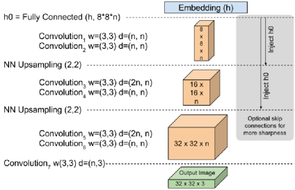
(a) Generator/Decoder

(b) Encoder

Figure 1: Network architecture for the generator and discriminator.

The structure is shown in figure 1. We used $3\times 3$ convolutions with exponential linear units [4] (ELUs) applied at their outputs. Each layer is repeated a number of times (typically 2). We observed that more repetitions led to even better visual results. The convolution filters are increased linearly with each down-sampling. Down-sampling is implemented as sub-sampling with stride 2 and up-sampling is done by nearest neighbor. At the boundary between the encoder and the decoder, the tensor of processed data is mapped via fully connected layers, not followed by any non-linearities, to and from an embedding state $h\in\mathbb{R}^{N_{h}}$ where $N_{h}$ is the dimension of the auto-encoder’s hidden state.

The generator $G:\mathbb{R}^{N_{z}}\mapsto\mathbb{R}^{N_{x}}$ uses the same architecture (though not the same weights) as the discriminator decoder. We made this choice only for simplicity. The input state is $z\in\left[-1,1\right]^{N_{z}}$ sampled uniformly.

3.5.1 Optional improvements

This simple architecture achieves high quality results and demonstrates the robustness of our technique.

Further, optional, refinements aid gradient propagation and produce yet sharper images. Taking inspiration from deep residual networks [8], we initialize the network using vanishing residuals: for successive same sized layers, the layer’s input is combined with its output: $in_{x+1}=carry\times in_{x}+(1-carry)\times out_{x}$. In our experiments, we start with $carry=1$ and progressively decrease it to 0 over 16000 steps (one epoch).

We also introduce skip connections [8, 17, 9] to help gradient propagation [3]. The first decoder tensor $h0$ is obtained from projecting $h$ to an $8\times 8\times n$ tensor. After each upsampling step, the output is concatenated with $h0$ upsampled to the same dimensions. This creates a skip connection between the hidden state and each successive upsampling layer of the decoder.

We did not explore other techniques typically used in GANs, such as batch normalization, dropout, transpose convolutions or exponential growth for convolution filters, though they might further improve upon these results.

4 Experiments

4.1 Setup

We trained our model using Adam with an initial learning rate of $0.0001$, decaying by a factor of $2$ when the measure of convergence stalls. Modal collapses or visual artifacts were observed sporadically with high initial learning rates, however simply reducing the learning rate was sufficient to avoid them. We trained models for varied resolutions from $32$ to $256$, adding or removing convolution layers to adjust for the image size, keeping a constant final down-sampled image size of $8\times 8$. We used $N_{h}=N_{z}=64$ in most of our experiments with this dataset.

Our biggest model for $128\times 128$ images used a convolution with $n=128$ filters and had a total of $17.3\times 10^{6}$ trainable parameters. Training time was about $2.5$ days on four P100 GPUs. Smaller models of size $32\times 32$ could train in a few hours on a single GPU.

We use a dataset of $360K$ celebrity face images for training in place of CelebA [12]. This dataset has a larger variety of facial poses, including rotations around the camera axis. These are more varied and potentially more difficult to model than the aligned faces from CelebA, presenting an interesting challenge. We preferred the use of faces as a visual estimator since humans excel at identifying flaws in faces.

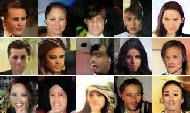
(a) EBGAN (64x64)

(b) Our results (128x128)

Figure 2: Random samples comparison

4.2 Image diversity and quality

Figure 2b shows some representative samples drawn uniformly from $z$ at resolutions of $128\times 128$. Higher resolution images, while maintaining coherency, tend to lose sharpness, but this may be improved upon with additional hyper-parameter explorations. To our knowledge these are the first anatomically coherent high-resolution results except for Stacked GANs [20] which has shown some promise for flowers and birds at up to $256\times 256$.

We observe varied poses, expressions, genders, skin colors, light exposure, and facial hair. However we did not see glasses, we see few older people and there are more women than men. For comparison we also displayed some EBGAN [21] results in figure 2a. We must keep in mind that these are trained on different datasets so direct comparison is difficult.

Figure 3: Random 64x64 samples at varying $\gamma\in\left\{0.3,0.5,0.7\right\}$

In Figure 3, we compared the effect of varying $\gamma$. The model appears well behaved, still maintaining a degree of image diversity across the range of values. At low values, the faces look overly uniform. Variety increases with $\gamma$ but so do artifacts. Our observations seem to contradict those of [14] that diversity and quality were independent.

4.3 Space continuity

To estimate the modal coverage of our generator we take real images and find their corresponding $z_{r}$ embedding for the generator. This is done using Adam to find a value for $z_{r}$ that minimizes $e_{r}=|x_{r}-G(z_{r})|$. Mapping to real images is not the goal of the model but it provides a way of testing its ability to generalize. By interpolating the $z_{r}$ embeddings between two real images, we verify that the model generalized the image contents rather than simply memorizing them.

(a) ALI [5] (64x64)

(b) Conditional PixelCNN [13] (32x32)

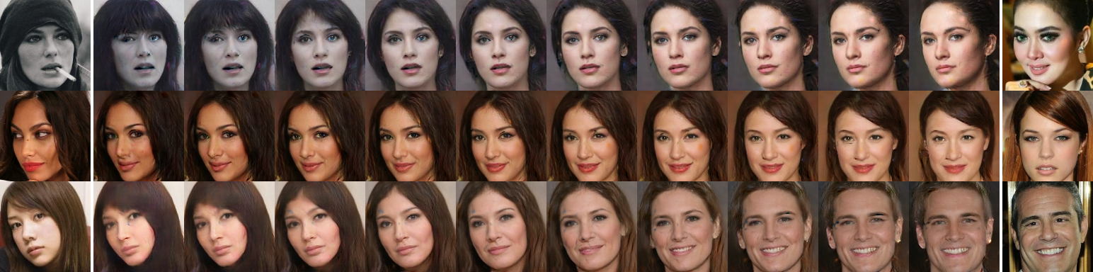
(c) Our results (128x128 with 128 filters)

(d) Mirror interpolations (our results 128x128 with 128 filters)

Figure 4: Interpolations of real images in latent space

Figure 4c displays interpolations on $z_{r}$ between real images at $128\times 128$ resolution; these images were not part of the training data. The first and last columns contain the real images to be represented and interpolated. The images immediately next to them are their corresponding approximations while the images in-between are the results of linear interpolation in $z_{r}$. For comparison with the current state of the art for generative models, we included ALI [5] results at $64\times 64$ (figure 4a) and conditional PixelCNN [13] results at $32\times 32$ (figure 4b) both trained on different data sets (higher resolutions were not available to us for these models). In addition figure 4d showcases interpolation between an image and its mirror.

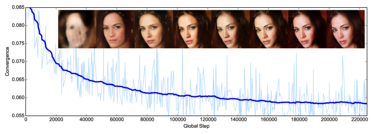
Figure 5: Quality of the results w.r.t. the measure of convergence (128x128 with 128 filters)

Sample diversity, while not perfect, is convincing; the generated images look relatively close to the real ones. The interpolations show good continuity. On the first row, the hair transitions in a natural way and intermediate hairstyles are believable, showing good generalization. It is also worth noting that some features are not represented such as the cigarette in the left image. The second and last rows show simple rotations. While the rotations are smooth, we can see that profile pictures are not captured as well as camera facing ones. We assume this is due to profiles being less common in our dataset. Finally the mirror example demonstrates separation between identity and rotation. A surprisingly realistic camera-facing image is derived from a single profile image.

4.4 Convergence measure and image quality

The convergence measure $\mathcal{M}_{global}$ was conjectured earlier to measure the convergence of the BEGAN model. As can be seen in figure 5 this measure correlates well with image fidelity. We can also see from this plot that the model converges quickly, just as was originally reported for EBGANs. This seems to confirm the fast convergence property comes from pixel-wise losses.

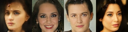
(a) Starved generator ($z=16$ and $h=128$)

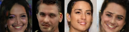
(b) Starved discriminator ($z=128$ and $h=16$)

Figure 6: Advantaging one network over the other

4.5 Equilibrium for unbalanced networks

To test the robustness of the equilibrium balancing technique, we performed an experiment advantaging the discriminator over the generator, and vice versa. Figure 6 displays the results.

By maintaining the equilibrium the model remained stable and converged to meaningful results. The image quality suffered as expected with low dimensionality of $h$ due to the reduced capacity of the discriminator. Surprisingly, reducing the dimensionality of $z$ had relatively little effect on image diversity or quality.

4.6 Numerical experiments

Method (unsupervised)	Score
Real data	11.	24
DFM [19]	7.	72
BEGAN (ours)	5.	62
ALI [5]	5.	34
Improved GANs [16]	4.	36
MIX + WGAN [2]	4.	04

Table 1: Inception scores (higher is better)

To measure quality and diversity numerically, we computed the inception score [16] on CIFAR-10 images. The inception score is a heuristic that has been used for GANs to measure single sample quality and diversity on the inception model. We train an unconditional version of our model and compare to previous unsupervised results. The goal is to generate a distribution that is representative of the original data.

A comparison to similar works on models trained entirely unsupervised is shown in table 1. With the exception of Denoising Feature Matching [19] (DFM), our score is better than other GAN techniques that directly aim to match the data distribution. This seems to confirm experimentally that matching loss distributions of the auto-encoder is an effective indirect method of matching data distributions. DFM appears compatible with our method and combining them is a possible avenue for future work.

5 Conclusion

There are still many unexplored avenues. Does the discriminator have to be an auto-encoder? Having pixel-level feedback seems to greatly help convergence, however using an auto-encoder has its drawbacks: what latent space size is best for a dataset? When should noise be added to the input and how much? What impact would using other varieties of auto-encoders such Variational Auto-Encoders[11] (VAEs) have?

More fundamentally, we note that our objective bears a superficial resemblance to the WGAN [1] objective. Is the auto-encoder combined with the equilibrium concept fulfilling a similar bounding functionality as the K-Lipschitz constraint in the WGAN formulation?

We introduced BEGAN, a GAN that uses an auto-encoder as the discriminator. Using proportional control theory, we proposed a novel equilibrium method for balancing adversarial networks. We believe this method has many potential applications such as dynamically weighing regularization terms or other heterogeneous objectives. Using this equilibrium method, the network converges to diverse and visually pleasing images. This remains true at higher resolutions with trivial modifications. Training is stable, fast and robust to parameter changes. It does not require a complex alternating training procedure. Our approach provides at least partial solutions to some outstanding GAN problems such as measuring convergence, controlling distributional diversity and maintaining the equilibrium between the discriminator and the generator. While we could partially control the diversity of generator by influencing the discriminator, there is clearly still room for improvement.

References

- [1] Martin Arjovsky, Soumith Chintala, and Léon Bottou. Wasserstein gan. arXiv preprint arXiv:1701.07875, 2017.
- [2] Sanjeev Arora, Rong Ge, Yingyu Liang, Tengyu Ma, and Yi Zhang. Generalization and equilibrium in generative adversarial nets (gans). arXiv preprint arXiv:1703.00573, 2017.
- [3] Yoshua Bengio, Patrice Simard, and Paolo Frasconi. Learning long-term dependencies with gradient descent is difficult. IEEE transactions on neural networks, 5(2):157–166, 1994.
- [4] Djork-Arné Clevert, Thomas Unterthiner, and Sepp Hochreiter. Fast and accurate deep network learning by exponential linear units (elus). arXiv preprint arXiv:1511.07289, 2015.
- [5] Vincent Dumoulin, Ishmael Belghazi, Ben Poole, Alex Lamb, Martin Arjovsky, Olivier Mastropietro, and Aaron Courville. Adversarially learned inference. arXiv preprint arXiv:1606.00704, 2016.
- [6] Ian Goodfellow. Nips 2016 tutorial: Generative adversarial networks. arXiv preprint arXiv:1701.00160, 2016.
- [7] Ian Goodfellow, Jean Pouget-Abadie, Mehdi Mirza, Bing Xu, David Warde-Farley, Sherjil Ozair, Aaron Courville, and Yoshua Bengio. Generative adversarial nets. In Advances in neural information processing systems, pages 2672–2680, 2014.
- [8] Kaiming He, Xiangyu Zhang, Shaoqing Ren, and Jian Sun. Deep residual learning for image recognition. In Proceedings of the IEEE Conference on Computer Vision and Pattern Recognition, pages 770–778, 2016.
- [9] Gao Huang, Zhuang Liu, Kilian Q Weinberger, and Laurens van der Maaten. Densely connected convolutional networks. arXiv preprint arXiv:1608.06993, 2016.
- [10] Diederik Kingma and Jimmy Ba. Adam: A method for stochastic optimization. arXiv preprint arXiv:1412.6980, 2014.
- [11] Diederik P Kingma and Max Welling. Auto-encoding variational bayes. arXiv preprint arXiv:1312.6114, 2013.
- [12] Ziwei Liu, Ping Luo, Xiaogang Wang, and Xiaoou Tang. Deep learning face attributes in the wild. In Proceedings of International Conference on Computer Vision (ICCV), 2015.
- [13] Aaron van den Oord, Nal Kalchbrenner, Oriol Vinyals, Lasse Espeholt, Alex Graves, and Koray Kavukcuoglu. Conditional image generation with pixelcnn decoders. arXiv preprint arXiv:1606.05328, 2016.
- [14] Ben Poole, Alexander A Alemi, Jascha Sohl-Dickstein, and Anelia Angelova. Improved generator objectives for gans. arXiv preprint arXiv:1612.02780, 2016.
- [15] Alec Radford, Luke Metz, and Soumith Chintala. Unsupervised representation learning with deep convolutional generative adversarial networks. arXiv preprint arXiv:1511.06434, 2015.
- [16] Tim Salimans, Ian Goodfellow, Wojciech Zaremba, Vicki Cheung, Alec Radford, and Xi Chen. Improved techniques for training gans. In Advances in Neural Information Processing Systems, pages 2226–2234, 2016.
- [17] Rupesh Kumar Srivastava, Klaus Greff, and Jürgen Schmidhuber. Highway networks. arXiv preprint arXiv:1505.00387, 2015.
- [18] Cédric Villani. Optimal transport: old and new, volume 338. Springer Science & Business Media, 2008.
- [19] D Warde-Farley and Y Bengio. Improving generative adversarial networks with denoising feature matching. ICLR submissions, 8, 2017.
- [20] Han Zhang, Tao Xu, Hongsheng Li, Shaoting Zhang, Xiaolei Huang, Xiaogang Wang, and Dimitris Metaxas. Stackgan: Text to photo-realistic image synthesis with stacked generative adversarial networks. arXiv preprint arXiv:1612.03242, 2016.
- [21] Junbo Zhao, Michael Mathieu, and Yann LeCun. Energy-based generative adversarial network. arXiv preprint arXiv:1609.03126, 2016.