Nonlinear Fluid Simulation Study of Stimulated Raman and Brillouin Scatterings in Shock Ignition

Abstract

We developed a new nonlinear fluid laser-plasma-instability code (FLAME) using a multi-fluid plasma model combined with full electromagnetic wave equations. The completed one-dimensional (1D) version of FLAME was used to study laser-plasma instabilities in shock ignition. The simulations results showed that absolute SRS modes growing near the quarter-critical surface were saturated by Langmuir-wave Decay Instabilities (LDI) and pump depletion. The ion-acoustic waves from LDI acted as seeds of Stimulated Brillouin Scattering (SBS), which displayed a bursting pattern and caused strong pump depletion. Re-scattering of SRS at the 1/16th-critical surface was also observed in a high temperature case. These results largely agreed with corresponding Particle-in-Cell simulations.

I Introduction

Laser-plasma instabilities (LPI) in inertial confinement fusion (ICF) include both convective and absolute modes. While absolute modes can grow to large amplitudes locally and are saturated by nonlinear effects, convective modes growth is limited by density gradients and their saturation amplitudes are the product of the seed level and the so-called Rosenbluth gain Rosenbluth72 . In recent particle-in-cell (PIC) simulations of LPI in a new ignition scheme, shock ignition Betti07 , convective and absolute modes were found both important. Laser reflectivity was found largely due to convective stimulated Brillouin scattering (SBS) below the quarter-critical surface Riconda11 ; Weber12 ; Weber15 ; Hao16 . Hot electrons were generated by absolute two plasmon decay (TPD) and stimulated Raman scattering (SRS) modes near the quarter-critical surface Riconda11 ; Weber12 ; Weber15 ; Yan14 . Convective SRS was also found below the quarter-critical surface Riconda11 ; Weber12 accompanied by significant changes in the electron distribution function and corresponding Landau damping Riconda11 . However it was not clear how the convective SRS can grow to such large amplitudes to alter the electron distribution function. In a recent 1D PIC simulations with a long density scale Hao16 , convective SRS was also found to contribute to the laser reflectivity at a higher level than that from fluid calculation based on a Thomson scattering seed level model Berger89 and the the Rosenbluth gain. It was found that the seed levels for both convective SBS and SRS in the PIC simulations were 4-7 orders of magnitude higher than the thermal noise Hao16 . However, the fluid calculation in Hao16 with a ray-based steady-state code HLIP Hao14 did not include the effects of the absolute SRS near the quarter-critical surface. It was not clear whether the high SRS reflectivity in the PIC simulations was entirely due the high seed levels. It was also not clear whether the large SBS reflectivity in the PIC simulations was influenced by the high seed levels.

To bridge the gap between full PIC simulations and steady-state fluid simulation on laser-plasma instabilities in ICF, especially in shock ignition, we developed a new nonlinear FLuid code of lAser-plasMa instabilitiEs (FLAME). To make the physics as close to PIC simulations as possible, we use the full wave equations for vector potentials of light without envelope approximations. Thus no particular mode would be precluded. The plasma is represented by an electron species and multiple ion species. Landau damping for both electrons and ions is evaluated in the spectral-space and included in the momentum equations for each species. Our model is in principle multi-dimensional (see the Appendix for detail) and can allow all three major LPI modes (SRS, SBS, and TPD). In this paper we report the implementation and benchmark of a one-dimension (1D) parallel version of FLAME and some simulation results on SRS and SBS in the shock ignition regime. Similar to the PIC simulations Hao16 , absolute SRS near the quarter-critical surface were observed to saturate via Langmuir wave decay instability (LDI) Karttunen81 and pump depletion. Re-scattering of the absolute SRS was also observed when the electron temperature was high. Laser reflectivity due to convective SRS was much smaller than in the PIC simulations, due to the seed level difference. The SBS reflectivity was similar to that in the PIC simulations and is the main cause for pump depletion. Through a contrasting simulation, we concluded that some ion acoustic wave modes generated in LDI acted as seeds for SBS, resulting bursting patterns in both SBS and transmitted light.

II Implementation of the 1D Version of FLAME

Details of our physics model are presented in the Appendix. In 1D, Eqs. (46)-(53) in the Appendix can be written in a dimensionless form as

$$\left({\frac{{{\partial^{2}}}}{{\partial{t^{2}}}}+{\nu_{c0}}\frac{\partial}{{\partial t}}-\frac{{{\partial^{2}}}}{{\partial{x^{2}}}}+{n_{A}}}\right){A_{0}}=-{n_{L}}{A_{1}},$$ (1)

$$\left({\frac{{{\partial^{2}}}}{{\partial{t^{2}}}}+{\nu_{c1}}\frac{\partial}{{\partial t}}-\frac{{{\partial^{2}}}}{{\partial{x^{2}}}}+{n_{A}}}\right){A_{1}}=-{n_{L}}{A_{0}},$$ (2)

$$\frac{{\partial{n_{L}}}}{{\partial t}}=-\frac{\partial}{{\partial x}}({n_{A}}{u_{Lx}}+{n_{L}}{u_{Ax}}),$$ (3)

$$\frac{{\partial{u_{Lx}}}}{{\partial t}} + ({\nu_{ce}}+2{\nu_{Le}}){u_{Lx}}$$

$$= \frac{\partial}{{\partial x}}({\phi_{L}}-{A_{0}}{A_{1}}-{u_{Ax}}{u_{Lx}})$$

$$-\frac{{{3}}}{{{n_{A}}}}\frac{\partial}{{\partial x}}({T_{e}}{n_{L}})+S_{L},$$

$$\frac{{{\partial^{2}}}}{{\partial{x^{2}}}}{\phi_{L}}={n_{L}},$$ (5)

$${n_{A}}=\sum\limits_{j}{{Z_{j}}{n_{j}}},$$ (6)

$${n_{A}}{u_{Ax}}=\sum\limits_{j}{{Z_{j}}{n_{j}}}{u_{jx}},$$ (7)

$$\frac{{\partial{n_{j}}}}{{\partial t}}=-\frac{\partial}{{\partial x}}({n_{j}}{u_{jx}}),$$ (8)

$$\frac{{\partial{u_{jx}}}}{{\partial t}} + ({\nu_{cj}}+2{\nu_{Lj}}){u_{jx}}+\frac{1}{2}\frac{\partial}{{\partial x}}u_{jx}^{2}$$

$$= -\frac{{{Z_{j}}}}{{{m_{j}}{n_{A}}}}\frac{\partial}{{\partial x}}({T_{e}}{n_{A}})-\frac{{{3}}}{{{m_{j}}{n_{j}}}}\frac{\partial}{{\partial x}}({T_{j}}{n_{j}})$$

$$-\frac{1}{2}\frac{{{Z_{j}}}}{{{m_{j}}}}\frac{\partial}{{\partial x}}(u_{Lx}^{2}+A_{0}^{2}+A_{1}^{2})+S_{j}.$$

Here, the normalized vector potential $A_{0}$ represents the incident laser and all scattered light that is not primary SRS, including SBS and the re-scattering of SRS, and $A_{1}$ represents the scattered light from the primary SRS. The normalized electron density $n_{A,L}$ and velocity $u_{A,Lx}$ represent the electron response on the ion acoustic scale (A) and Langmuir wave scale (L). The normalized ion density, velocity, mass, and charge state for species $j$ are $n_{j},u_{jx},m_{j}$ and $Z_{j}$, respectively. Both the collisional ($\nu_{c}$) and Landau ($\nu_{L}$) damping are included. The normalized units of density, time, length, velocity, mass, temperature, vector potential and static electric potential are $n_{c}$, $1/\omega_{0}$, $c/\omega_{0}$, $c$, $m_{e}$, $m_{e}c^{2}$, $m_{e}c^{2}/e$ and $m_{e}c^{2}/e$ respectively, where $n_{c}$ is the critical density and $\omega_{0}$ is the frequency of the incident laser. $S_{L}$ and $S_{j}$ are random fluctuating source terms with the magnitudes approximating to thermal noise. The 1D model was implemented in four parts including the electromagnetic (EM) wave solver, the electron response solver, the ion response solver, and the Landau damping solver.

In the EM wave solver, Eqs. (1) and (2) were discretized by the central difference scheme. Laser was launched from an antenna at the left boundary of the physical domain. The perfectly matched layer (PML) technique Berenger94 was used as the absorption boundary conditions at both sides of the physical domain.

For the electron response solver, Eq. (II) was separated into

$$\frac{{\partial{u_{Lx}}}}{{\partial t}}+\nu_{ce}{u_{Lx}} = \frac{\partial}{{\partial x}}({\phi_{L}}-{A_{0}}{A_{1}}-{u_{Ax}}{u_{Lx}})$$

$$-\frac{{{3}}}{{{n_{A}}}}\frac{\partial}{{\partial x}}({T_{e}}{n_{L}})+S_{L},$$

$$\frac{{\partial{u_{Lx}}}}{{\partial t}}+2{\nu_{Le}}{u_{Lx}}=0,$$ (11)

based on the time-splitting method Strang68 . Equations (3) and (II) were solved together using a leapfrog scheme. Equation (11) was solved in a Landau damping solver described later in this section. The Poisson equation (5) was solved as a tri-diagonal matrix equation in the entire simulation box.

Similarly, for the ion response solver, Eq. (II) was separated into

$$\frac{{\partial{u_{jx}}}}{{\partial t}} = -\frac{1}{2}\frac{\partial}{{\partial x}}u_{jx}^{2}$$

$$-\frac{{{Z_{j}}}}{{{m_{j}}{n_{A}}}}\frac{\partial}{{\partial x}}({T_{e}}{n_{A}})-\frac{{{3}}}{{{m_{j}}{n_{j}}}}\frac{\partial}{{\partial x}}({T_{j}}{n_{j}})$$

$$-\frac{1}{2}\frac{{{Z_{j}}}}{{{A_{j}}{m_{p}}}}\frac{\partial}{{\partial x}}(u_{Lx}^{2}+A_{0}^{2}+A_{1}^{2})+S_{j},$$

$$\frac{{\partial{u_{jx}}}}{{\partial t}}+({\nu_{cj}}+2{\nu_{Lj}}){u_{jx}}=0,$$ (13)

based on the time-splitting method. Equations (13) was also solved in the Landau damping solver. Since $u_{jx}$ includes both the background flow velocity and the perturbation components that are the ion-acoustic waves, the collisional damping ($\nu_{cj}$) was included in Eqs. (13), which was solved in the spectral space, to apply only on the modes with nonzero wavenumbers. For each time step, after calculating Eqs. (6) and (7) locally, Eqs. (8) and (II) were solved together using the leapfrog scheme in both the physics domain and the PML layers with the boundary condition $\partial^{2}n_{j}/\partial x^{2}=0$ and $\partial^{2}u_{jx}/\partial x^{2}=0$.

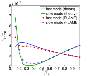
(a) (b)

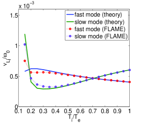
Figure 1: (Color online) Effective Landau damping rates for two modes of the weekly damped ion-acoustic wave in FLAME code with (a) $T_{e}=1.6$keV, $n_{e}=0.2n_{c}$, $k\lambda_{D}=0.224$ and (b) $T_{e}=3.5$keV, $n_{e}=0.2n_{c}$, $k\lambda_{D}=0.331$.

In the Landau damping solver, Eqs. (11) and (13) were solved in the spectral ($k$-)space using a real-space moving window. Fast Fourier Transform (FFT) was performed in the window to calculate Landau damping rates of the electron plasma waves and the ion-acoustic waves according to the average density and temperature in the window using Eqs. (14) and (15). Then inverse FFT was performed to obtain the damped value of $u_{Lx}$ and $u_{jx}$ at this point in the real space. In the current 1D version, the Landau damping rates were

$${\nu_{Le}}(k)=\sqrt{\frac{\pi}{8}}\frac{\omega_{pe}}{{(k{\lambda_{D}})^{3}}}\exp\left[{-\frac{1}{2{(k{\lambda_{D}})}^{2}}-\frac{3}{2}}\right],$$ (14)

for the electron plasma wave Landau46 and

$$\nu_{Lj}(k)=\sqrt{\frac{\pi}{8}}\omega_{j}(k)\left(\frac{Z_{j}}{m_{j}}\right)^{1/2}$$ (15)

$$+\sqrt{\frac{\pi}{8}}\omega_{j}(k)\left(\frac{Z_{j}T_{e}}{T_{j}}\right)^{3/2}\exp\left[-\frac{Z_{j}T_{e}}{2T_{j}(1+k^{2}\lambda_{D}^{2})}-\frac{3}{2}\right]$$

for the single ion species case Fried61 , where $\omega_{j}=k\sqrt{{Z_{j}}{T_{e}}/{m_{j}}(1+k^{2}\lambda_{D}^{2})+3T_{j}/m_{j}}$ and $\lambda_{D}$ is the electron Debye length. For cases with two ion species, analytic formula of Landau damping rates for different modes of the weakly damped ion-acoustic waves vu94 are available. Since we solved the equations of different ion species, not different modes of the ion-acoustic wave, in our model, we had to choose Landau damping rates for different ion species approximately. Currently, in FLAME, the analytic formula of Landau damping rate for the slow mode vu94 was used as the Landau damping rate of the heavy ion species and the analytic formula of Landau damping rate for the fast mode vu94 was used as the Landau damping rate of the light ion species. By solving the eigenvalue equation for the ion-acoustic modes Williams95 with these Landau damping rates, we can obtain the effective Landau damping rates for the fast and slow modes in our fluid model. Examples of a CH-plasma with fully ionized C and H in $1:1$ ratio are shown in Figs. 1(a) and 1(b) for different $T_{e}$ and $k\lambda_{D}$, where the effective Landau damping rates of two different modes were close to their theoretical value obtained by the analytic formula vu94 . So the approximation in Landau damping solver for two ion species was reasonable for most of temperature conditions.

III Benchmark of 1D FLAME Code

The 1D FLAME code was benchmarked by simulating the reflectivity of single SRS and single SBS modes under different laser intensities in a uniform hydrogen plasma in the heavily damped regime. The plasma parameters were chosen as $n_{e}=0.1n_{c}$, $T_{e}=3.5$keV, $T_{i}=1.6$keV, with the incident laser wavelength of $\lambda_{0}=0.351\mu$m. The length of the physical domain was $L=4000c/\omega_{0}$. In this regime, the reflectivity can be predicted by a theoretical formula

$$R(1-R)=\varepsilon[{e^{G(1-R)}}-R],$$ (16)

where $G$ is the gain factor of the corresponding instability Tang66 . For a single SRS mode,

$$G_{R}=\frac{\omega_{pe}^{2}k_{L}^{2}v_{os}^{2}L}{8\omega_{R}\omega_{L}\nu_{Le}v_{gR}},$$ (17)

and for a single SBS mode,

$$G_{B}=\frac{Z_{j}m_{e}\omega_{pe}^{2}k_{A}^{2}v_{os}^{2}L}{8m_{j}\omega_{B}\omega_{A}\nu_{Lj}v_{gB}},$$ (18)

where $\omega_{R}$, $\omega_{L}$, $\omega_{B}$ and $\omega_{A}$ are the best matching frequency of the SRS backscattered light, the Langmuir wave, the SBS backscattered light and the ion-acoustic wave respectively, $k_{L}$ and $k_{A}$ are the best matching wavenumber of the Langmuir wave and the ion-acoustic wave, $v_{gR}$ and $v_{gB}$ are the group velocities of the backscattered light in SRS and SBS respectively, and $v_{os}$ is the electron quiver velocity Tang66 ; Hao13 .

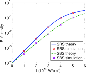
Figure 2: (Color online) Reflectivity versus laser intensity in the benchmark simulations.

In this regime, Landau damping dominates over collisional damping, which was neglected in the benchmark. In these benchmark simulations, we turned off either the ion response part or the electron response part to simulate pure SRS or SBS, respectively. The reflectivity in the simulations was measured at the left boundary of the physical domain, where the incident laser was launched, using $R={k_{s}}{A_{s}}{(0)^{2}}/{k_{0}}{A_{0}}{(0)^{2}}$ where $k_{s}$ and $A_{s}$ denote the wavenumber and amplitude of the backscattered light, respectively, and $k_{0}$ and $A_{0}$ that of the incident light. Seeds were launched from another antenna at the right boundary with the resonant frequency of the mode under study. The seed level in Eq. (16) is defined as $\varepsilon={k_{s}}{A_{s}}{(L)^{2}}/{k_{0}}{A_{0}}{(0)^{2}}$, which was chosen to be $\varepsilon=10^{-4}$ in these simulations. In Fig. 2, the solid blue curve and the dash-dot green curve show the theoretical reflectivities of SRS and SBS, respectively. The red circles and the purple squares are the relevant simulation results of the 1D FLAME code. The good agreement between the simulations and the theory shows that at least in this regime, the code modeled the correct physics in exciting and damping of SRS and SBS and also pump depletion of the incident laser.

IV The Simulations for LPI in Shock Ignition

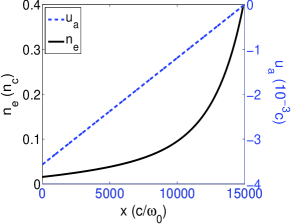
Figure 3: (Color online) The normalized density profile (black solid line) and plasma flow profile (blue dashed line) used in the simulations.

The 1D FLAME code was used to study SBS and SRS in shock ignition. These new fluid simulations adopted the same laser and plasma parameters of the 40+20-beam experiment on OMEGA Theobald12 that was simulated in Ref. Hao16 . Figure 3 shows the initial density profile and the plasma flow profile Hao16 , fitted from the LILAC Delettrez simulations, in the physical domain of our simulations. The incident laser had a wavelength of $\lambda_{0}=0.351\mu m$. The entire simulation box length was $16000c/\omega_{0}$, including the length of the physical domain $L=15000c/\omega_{0}$ (about $836\mu$m) and two PML layers of $L_{l}=500c/\omega_{0}$ each at the left and right boundaries. In the physical domain, the density ranged from $0.0156n_{c}$ to $0.4n_{c}$ with a scale length of $L_{n}=170\mu$m near the $1/4-n_{c}$ surface. Two ion species were fully ionized C and H in 1:1 ratio. Two sets of typical plasma temperatures were used Hao16 . At the launch of the ignition pulse, $T_{e}=1.6$keV and $T_{C}=T_{H}=0.55$keV, denoted here as the low temperature (LT) case . At the peak intensity of the ignition pulse, $T_{e}=3.5$keV and $T_{C}=T_{H}=1.6$keV, denoted here as the high temperature (HT) case. The grid size was $\Delta x=0.2c/\omega_{0}$ and the time step was $\Delta t=0.18/\omega_{0}$ for both LT and HT cases.

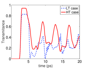
Figure 4: (Color online) Transmittance of laser intensity versus time.

For the temperature ratio $T_{i}/T_{e}\approx 0.34$ in the LT case and $T_{i}/T_{e}\approx 0.46$ in the HT case, the slow mode of the ion-acoustic wave in the CH plasma has a lower Landau damping rate than the fast mode as shown in Fig. 1. Therefore the slow mode should be the dominant mode and its damping is higher in HT than in LT.

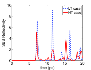
(a) (b)

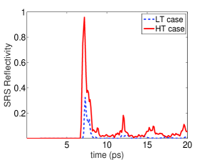
Figure 5: (Color online) Reflectivity of (a) SBS and (b) SRS versus time.

To frequency resolve the incident and backscattered light in FLAME, $A_{0}$ and $A_{1}$ were dumped every $15$ time steps. Through 2D FFT in time-space windows, the incident and backscattered light can be separated in the $\omega-k$ phase space. For diagnosis of the laser transmittance to $n=0.17n_{c}$, such 2D FFT windows were chosen in the region of $0.16\sim 0.18n_{c}$ with $2100\Delta x$ in space and $3000\Delta t$ in time (Fig.4). For diagnosis of the reflectivity, the 2D FFT windows were chosen at the left boundary of the physical domain with $5000\Delta x$ in space and $3000\Delta t$ in time (Fig.5).

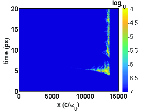
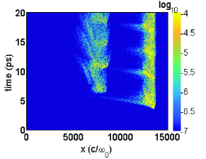
(a) (c)
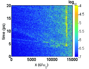
(b) (d)

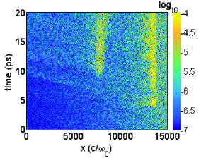
Figure 6: (Color online) Evolution of $n_{L}^{2}$ in fluid simulations for the (a) LT and (b) HT cases and evolution of $E_{x}^{2}$ in PIC simulations for the (c) LT and (d) HT cases.

Table 1: Average transmittance and reflectivity

		Temperature		FLAME		OSIRIS
Transmittance		LT case		$26\%$		$20\%$
		HT case		$38\%$		$32\%$
SBS reflectivity		LT case		$49\%$		$51\%$
		HT case		$41\%$		$31\%$
SRS reflectivity		LT case		$1.1\%$		$13\%$
		HT case		$5.6\%$		$25\%$

Simulations of both the HT and LT cases were performed for $20$ps with $I=5\times 10^{15}$W/cm². Figure 4 shows the fraction of the incident laser intensity arriving at the region of $0.16\sim 0.18n_{c}$ as a function of time. Significant pump depletion started at about $4$ps, and the transmittance was intermittent and was lower in the LT case. Reflectivities of SBS and SRS are shown in Figs. 5(a) and 5(b), respectively. Bursting SBS reflectivity had very high instantaneous peaks and was stronger in the LT case, due to the lower Landau damping rate of the ion-acoustic wave, than the HT case. The SRS reflectivity was largest in the the first peak and was significantly smaller than SBS. Therefore SBS was the main cause for the significant pump depletion. The temporal-averaged transmittance and reflectivities are listed in Table 1, together with the results from OSIRIS Fonseca02 PIC simulations of the same conditions. Both FLAME and OSIRIS simulations found similar transmittance and SBS reflectivities in both the LT and HT cases. They both found lower transmittance, stronger SBS, and weaker SRS in the LT case than in the HT case. The two types of simulations showed similar physical trends. One significant difference is that the FLAME simulations showed a much lower SRS reflectivity than the OSIRIS simulations. The high SRS reflectivity in the OSIRIS simulation was previously shown partly due to the strong convective modes in the low density region that were influenced by the inflated seed levels Hao16 . In the fluid simulations, we set the magnitude of seeds in FLAME code to be about $10^{-9}n_{c}$, the level of thermal noises Berger98 . Without the inflated seed level, SRS was dominated by the absolute modes.

(a) (b)

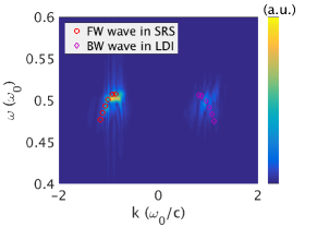
Figure 7: (Color online) $\omega-k$ space of $n_{L}$ near $(1/4)n_{c}$ for the (a) LT and (b) HT cases.

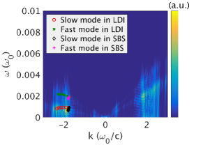
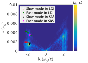
(a) (c)
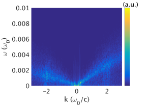
(b) (d)

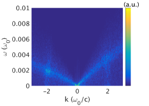
Figure 8: (Color online) $\omega-k$ space of perturbations of $n_{A}$ near $(1/4)n_{c}$ in fluid simulations for the (a) LT and (b) HT cases. $\omega-k$ space of perturbations of total charge density of ions near $(1/4)n_{c}$ in PIC simulations for the (c) LT and (d) HT cases.

In Figs. 6 we compare the plasma wave amplitudes in the FLAME and the OSIRIS simulations. In both simulations, absolute SRS first developed in a narrow region just below $n=1/4n_{c}$. Both simulations showed re-scattering of SRS near the region of $n=1/16n_{c}$ Klimo10 in the HT case but not in the LT. For the re-scattered SRS Langmuir waves near $1/16-n_{c}$, the collisional damping dominates over the Landau damping. The lower collisional damping in the HT case allowed the re-scattering. The saturation amplitudes of the plasma waves near the $1/4-n_{c}$ and the $1/16-n_{c}$ surfaces were also comparable in both types of simulations. All these are evidences that FLAME and OSIRIS modeled key physics of the absolute SRS in similar ways. Furthermore, the FLAME simulations did not show any significant convective SRS outside the narrow regions near the $1/4-n_{c}$ and the $1/16-n_{c}$ surfaces, unlike the OSIRIS simulations. We attribute this difference to the inflated seed levels in the PIC simulations Hao16 , which we believe was also the cause of the difference in the total SRS reflectivity in Table 1.

The absolute SRS near $1/4-n_{c}$ saturated due to pump depletion and LDI. Figures 7(a) and 7(b) show the spectra of the electron density associated with the Langmuir waves $n_{L}$ for the LT and HT cases respectively. The spectra were obtained by 2D FFT to $n_{L}$ in the region of $0.2\sim 0.26n_{c}$ and at $t=4.2$ps using a window of $4000\Delta x$ and $4500\Delta t$. In Figs. 7(a) and 7(b), modes in the left half ($k<0$) were forward (FW) propagating plasma waves, which were the daughter waves of the absolute SRS. These modes overlapped with the red circles representing the theoretical values of the SRS Langmuir waves calculated from the matching conditions in the region. And modes in the right half ($k>0$) were backward (BW) propagating plasma waves, which overlapped with the pink diamonds representing the theoretical values of the BW Langmuir waves calculated from the LDI dispersion relations Karttunen81 . These BW waves were the daughter waves of LDI.

Spectra of the ion acoustic waves, from the perturbations of $n_{A}$, were also obtained and shown in Figs. 8(a) and 8(b) for the LT and HT cases, respectively. The time duration of the 2D FFT window was chosen to be $300000\Delta t$. The forward (FW) ion-acoustic waves in the left half, including both the fast and slow modes, were from SBS and also from LDI. For our temperature conditions, the slow mode was the dominant one due to its smaller Landau damping rate Williams95 . Both slow and fast modes overlapped with the theoretical values for the the FW ion-acoustic wave induced by LDI (the red circles and the green stars) and by SBS (the black diamonds and the pink plus signs) in the region of $0.2\sim 0.26n_{c}$. The backward (BW) ion-acoustic waves in the right half were probably induced by secondary LDI of the BW Langmuir waves. The phase velocities of the FW and BW ion acoustic waves were different due to the Doppler shift from the background flow. These features in the spectra were largely also observed in the OSIRIS simulations (Figs. 8(c) and 8(d) for the LT and HT cases, respectively).

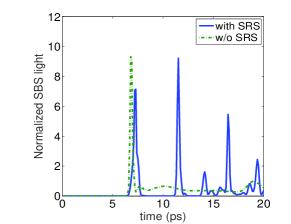
(a) (b)

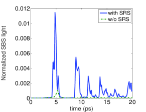
Figure 9: (Color online) Comparison of the normalized SBS light intensity (a) at the left boundary and (b) in the region of $0.2\sim 0.26n_{c}$ with and without SRS for the LT case.

Figures. 8(a) and 8(b) show that some modes of the ion-acoustic waves in LDI had similar frequencies and wavenumbers to the ion-acoustic waves in SBS near $0.25n_{c}$. This indicates that SBS can be seeded by the absolute SRS through LDI near $0.25n_{c}$, rather than by thermal noises. To further corroborate this, we did a contrasting simulation for the LT case, where the electron response was turned off to eliminate SRS. Without competition from SRS, the first peak of the SBS reflectivity was even slightly stronger (Fig. 9a). However after pump depletion took effect, the SBS reflectivity lost the bursting pattern and had a time-averaged SBS value of 45%, which was still significant and was mainly from the amplification of thermal noises in the entire box. In contrast, when SRS was present the seed levels in the $0.2-0.26n_{c}$ region were significantly higher (Fig. 9b) and had a bursting pattern. We believed they were induced by SRS-LDI near $0.25n_{c}$ and was the cause of the burst pattern of the SBS reflectivity in Fig. 9(a), which in turn caused the SRS bursts through pump depletion. Therefore even though the time averaged SBS reflectivities were similar with and without SRS, their origins were different. Thus we also conclude that the SBS reflectivity in the PIC simulations were mostly physical.

V Discussion and Summary

The simulations here and in previous studies Riconda11 ; Weber12 ; Weber15 ; Hao16 showed under various conditions relevant to shock ignition SBS was the dominant backscatter. However, experimental results Theobald12 showed above $I=4\times 10^{15}$W/cm² SRS reflectivity started to exceed the SBS reflectivity. The high intensity experimental shots used no phase plates Theobald12 . In addition, TPD can compete with absolute SRS near $0.25n_{c}$ and affect pump depletion and SBS seeding. Whether these factors would affect the relative strength in SBS and SRS reflectivities is an interesting research topic that can be studied when FLAME is extended to multi-dimensions.

In summary, we presented a physics model for laser-plasma instabilities in ICF that is fundamentally multi-dimensional, multi-fluid and full-wave. This model can be used to study coupling of major LPI’s with controllable noise sources, bridging envelope-based fluid simulations and full PIC simulations. The completed 1D version of a nonlinear fluid code FLAME based on this model was benchmarked and used to study the coupling of SBS and SRS for typical parameter conditions in shock ignition. Results showed strong bursts of SBS in both the low temperature and high temperature cases, which resulted in strong pump depletion. Absolute SRS near $0.25n_{c}$ saturated by LDI and pump depletion. Part of the ion-acoustic waves generated in LDI acted as an efficient seed for SBS. The coupling of SRS and SBS through seeding and pump depletion caused a bursting pattern in LPI activities. Re-scatter of SRS was also observed in the high temperature case near $1/16-n_{c}$. Most of the simulation results, with the exception of smaller convective SRS reflectivities due to different noise levels, were consistent with the PIC simulations. In general, the FLAME simulations were 5-10 times faster than the PIC simulations.

VI acknowledgments

The authors would like to acknowledge the OSIRIS Consortium for the use of OSIRIS. This work was supported by DOE under Grant No. DE-FC02-04ER54789 and DE-SC0012316; and by NSF under Grant No. PHY-1314734. The research used resources of the National Energy Research Scientific Computing Center. The support of DOE does not constitute an endorsement by DOE of the views expressed in this paper.

Rui Yan is also supported by National Natural Science Foundation of China (NSFC) under Grant No. 11621202, and No. 11642020; by the Strategic Priority Research Program of the Chinese Academy of Science (Grant No. XDB16); and by Science Challenge Project of China (No. JCKY2016212A505).

VII Appendix: The physics model

In this Appendix, we derive the physics model of FLAME. The starting point of this model is to group all relevant quantities according to their frequencies: 1. the ion acoustic wave frequency and smaller (subscripted $A$); 2. the plasma wave (Langmuir wave) frequency (subscripted $L$); and 3. the incident laser frequency (subscripted $0$), with the frequencies satisfying $\omega_{A}\ll\omega_{L}<0.5\omega_{0}$ in the underdense laser plasma interaction regimes. The frequencies of the scattered light, however, usually overlap with either $\omega_{0}$ (SBS) or $\omega_{L}$ (SRS).

Therefore, the relevant quantities can be decomposed as follows:

$$n_{e}=n_{A}+n_{L},$$ (19)

$$\phi=\phi_{A}+\phi_{L}+{\phi_{0}},$$ (20)

$$\vec{u}_{e}=\vec{u}_{A}+\vec{u}_{L}+\vec{v}_{os},$$ (21)

where $n_{e}$ is the electron density, $u_{e}$ is the electron velocity, and $\phi$ is the electro-static potential; $\vec{v}_{os}=\vec{v}_{0}+\vec{v}_{1}$ representing the electron oscillatory velocities under the incident light ($\vec{v}_{0}$) and the scattered light ($\vec{v}_{1}$).

This model is also based on the quasi-neutrality assumption,

$$n_{A}=\Sigma Z_{j}n_{j},$$ (22)

$$n_{A}\vec{u}_{A}=\Sigma Z_{j}n_{j}\vec{u}_{j},$$ (23)

where $Z_{j}$, $n_{j}$, and $\vec{u}_{j}$ are the charge number, number density, and velocity of the $j$th ion species, respectively.

VII.1 The laser propagation

The Maxwell’s equations:

$$\nabla\times\vec{E}=-\frac{1}{c}\frac{\partial\vec{B}}{\partial t},$$ (24)

$$\nabla\times\vec{B}=\frac{1}{c}\frac{\partial\vec{E}}{\partial t}+\frac{4\pi}{c}\vec{J},$$ (25)

$$\nabla\cdot\vec{E}=4\pi e(-n_{e}+\Sigma Z_{j}n_{j}),$$ (26)

$$\nabla\cdot\vec{B}=0.$$ (27)

are convenient to be written in the form of the vector potential $\vec{A}$ associated with laser field and the electrostatic potential $\phi$. The electric and magnetic fields are rewritten as

$$\vec{B}=\nabla\times\vec{A},$$ (28)

$$\vec{E}=-\frac{1}{c}\frac{\partial\vec{A}}{\partial t}-\nabla\phi.$$ (29)

With the Coulomb gauge $\nabla\cdot\vec{A}=0$, Eqs. (24) and (25) become

$$\frac{\partial^{2}\vec{A}}{\partial t^{2}}-c^{2}\nabla^{2}\vec{A}=-c\frac{\partial}{\partial t}\nabla\phi+4\pi c\vec{J}.$$ (30)

Using $\vec{v}_{0,1}=e\vec{A}_{0,1}/(mc)$, the current $\vec{J}=(-n_{e}\vec{u}_{e}+\Sigma Z_{j}n_{j}\vec{u}_{j})e$ can also be decomposed as

$$\vec{J} = -en_{A}(\vec{u}_{L}+\frac{e\vec{A}_{0}}{mc}+\frac{e\vec{A}_{1}}{mc})$$

$$-en_{L}(\vec{u}_{A}+\vec{u}_{L}+\frac{e\vec{A}_{0}}{mc}+\frac{e\vec{A}_{1}}{mc})$$

$$= \vec{J}_{0}+\vec{J}_{1},$$

where

$$\vec{J}_{0}=-e[n_{A}\frac{e\vec{A}_{0}}{mc}+n_{L}(\vec{u}_{L}+\frac{e\vec{A}_{1}}{mc})],$$ (32)

$$\vec{J}_{1}=-e[n_{A}(\vec{u}_{L}+\frac{e\vec{A}_{1}}{mc})+n_{L}(\vec{u}_{A}+\frac{e\vec{A}_{0}}{mc})].$$ (33)

Note that the ion acoustic component $\vec{J}_{A}$ has been cancelled due to Eq. (23).

Then Eq. (30) can be further decomposed and simplified as:

$$(\frac{\partial^{2}}{\partial t^{2}}-c^{2}\nabla^{2}+\omega_{pe}^{2})\vec{A}_{0}=-\frac{n_{L}}{n_{A}}\omega_{pe}^{2}\vec{A}_{1}-4\pi ecn_{L}\vec{u}_{L}-{c\frac{\partial}{\partial t}\nabla\phi_{0}},$$ (34)

$$(\frac{\partial^{2}}{\partial t^{2}}-c^{2}\nabla^{2}+\omega_{pe}^{2})\vec{A}_{1}=-c\frac{\partial}{\partial t}\nabla\phi_{L}-\frac{n_{L}}{n_{A}}\omega_{pe}^{2}\vec{A}_{0}-4\pi ec(n_{A}\vec{u}_{L}+n_{L}\vec{u}_{A}),$$ (35)

where $\omega_{pe}=4\pi n_{A}e^{2}/m$ is the local plasma frequency, $\nabla^{2}\phi_{L}=4\pi en_{L}$, and ${\partial\nabla\phi_{0}/\partial t=-4\pi\vec{J}_{0}}$, whose purpose is to ensure $\nabla\cdot A_{0}=0$.

VII.2 The electron evolution

The fluid equations for the electrons,

$$\frac{\partial n_{e}}{\partial t}+\nabla\cdot(n_{e}\vec{u}_{e})=0,$$ (36)

$$\frac{\partial\vec{u}_{e}}{\partial t}+\vec{u}_{e}\cdot\nabla\vec{u}_{e}=-\frac{1}{mn_{e}}\nabla p_{e}-\frac{e}{m}(\vec{E}+\frac{\vec{u}_{e}\times\vec{B}}{c}),$$ (37)

can be decomposed using Eqs. (19,20,21). The ion acoustic component of the electron mass equation is already taken care of by the quasi-neutrality conditions. It is straight forward to obtain the Langmuir time-scale component of Eq. (36):

$$\frac{\partial n_{L}}{\partial t}+\nabla\cdot[n_{A}\vec{u}_{L}+n_{A}\frac{e\vec{A}_{1}}{mc}+n_{L}\vec{u}_{A}+n_{L}\frac{e\vec{A}_{0}}{mc}]=0.$$ (38)

The simplification of the electron momentum equation needs an equation of state. Here the adiabatic condition for the electrons is used when handling the Langmuir waves, $[\nabla p_{e}]_{L}=\gamma T_{e}\nabla n_{L}$ where $\gamma$ is the adiabatic index. Use the identity: $\vec{a}\cdot\nabla\vec{a}\equiv(\nabla\times\vec{a})\times\vec{a}+\nabla(|a|^{2}/2)$, the Langmuir time-scale terms of Eq.(37) yield:

$$\frac{\partial\vec{u}_{L}}{\partial t} = \frac{e}{m}\nabla\phi_{L}-\nabla[(\frac{e\vec{A}_{0}}{mc}+\vec{u}_{A})\cdot(\vec{u}_{L}+\frac{e\vec{A}_{1}}{mc})]$$

$$-\gamma v_{th}^{2}\frac{\nabla n_{L}}{n_{A}}+(\vec{u}_{L}+\frac{e\vec{A}_{1}}{mc})\times\vec{\Omega}+{(\vec{u}_{A}+\frac{e\vec{A}_{0}}{mc})\times(\nabla\times\vec{u}_{L})},$$

where $v_{th}=\sqrt{T_{e}/m}$ is the electron thermal velocity, $\Omega=\nabla\times\vec{u}_{A}$ is the vorticity of the background (ion-acoustic time scale) velocity of this plasma.

Neglecting the electron inertia, the slow components of Eq. (37) become:

$$\frac{\partial\vec{u}_{A}}{\partial t}\approx 0=\frac{e}{m}\nabla\phi_{A}-\frac{1}{2}[\nabla(\vec{u}_{L}+\frac{e\vec{A}}{mc})^{2}]_{A}-\frac{[\nabla p_{e}]_{A}}{n_{e}m},$$ (40)

which provides the relation between the slow electron static field $\nabla\phi_{A}$ driving the ions and the quantities in faster time scales.

VII.3 The ion evolution

Excluding the ion quiver motions, the ion fluid equations are

$$\frac{\partial n_{j}}{\partial t}+\nabla\cdot(n_{j}\vec{u}_{j})=0,$$ (41)

$$\frac{\partial\vec{u}_{j}}{\partial t}+\vec{u}_{j}\cdot\nabla\vec{u}_{j}=-\frac{1}{M_{j}n_{j}}\nabla p_{j}-\frac{Z_{j}e}{M_{j}}\nabla\phi_{A},$$ (42)

Substitute Eq.(40) into Eq.(42), we obtain

$$\frac{\partial\vec{u}_{j}}{\partial t}+\vec{u}_{j}\cdot\nabla\vec{u}_{j}=-\frac{Z_{j}m}{M_{j}}(\frac{1}{2}[\nabla(\vec{u}_{L}+\frac{e\vec{A}}{mc})^{2}]_{A}+\frac{[\nabla p_{e}]_{A}}{n_{e}m})-\frac{\nabla p_{j}}{M_{j}n_{j}}.$$ (43)

Using the iso-thermal condition for the electrons $[\nabla p_{e}]_{A}=T_{e}\nabla n_{A}$ and the adiabatic condition for the ions $\nabla p_{j}/p_{j}=\gamma\nabla n_{j}/n_{j}$, we obtain

$$\frac{\partial\vec{u}_{j}}{\partial t}+\vec{u}_{j}\cdot\nabla\vec{u}_{j}=-\frac{Z_{j}m}{M_{j}}(\frac{1}{2}[\nabla(\vec{u}_{L}+\frac{e\vec{A}}{mc})^{2}]_{A})-\frac{Z_{j}T_{e}}{M_{j}}\frac{\nabla n_{A}}{n_{A}}-\frac{\gamma T_{j}}{M_{j}}\frac{\nabla n_{j}}{n_{j}}.$$ (44)

The term $\nabla[\vec{u}_{L}+e\vec{A}/(mc)]^{2}$ include components of multiple frequencies and we aim to only keep the slowest (ion-acoustic) components and drop the high-frequency parts as much as possible. So we rewrite Eq.(44) as:

$$\frac{\partial\vec{u}_{j}}{\partial t}+\vec{u}_{j}\cdot\nabla\vec{u}_{j}\\ =-\frac{Z_{j}m}{M_{j}}\frac{1}{2}\nabla[\vec{u}_{L}^{2}+(\frac{e\vec{A}_{0}}{mc})^{2}+(\frac{e\vec{A}_{1}}{mc})^{2}+2\vec{u}_{L}\cdot\frac{e\vec{A}_{1}}{mc}]-\frac{Z_{j}T_{e}}{M_{j}}\frac{\nabla n_{A}}{n_{A}}-\frac{\gamma T_{j}}{M_{j}}\frac{\nabla n_{j}}{n_{j}}.$$ (45)

Note that some high-frequency components still exist in the bracket. For example, $\vec{u}_{L}^{2}$ includes both the $\omega\approx 0$ and $\omega\approx 2\omega_{pe}$ components. However, the $2\omega_{pe}$ component is far off resonant in this equation and is expected not to grow very much.

Finally, we collect all the equations for this model, rewritten as follows:

1. For the light,

   $$(\frac{\partial^{2}}{\partial t^{2}}-c^{2}\nabla^{2}+\omega_{pe}^{2})\vec{A}_{0}=-\frac{n_{L}}{n_{A}}\omega_{pe}^{2}\vec{A}_{1}-4\pi ecn_{L}\vec{u}_{L}-{c\frac{\partial}{\partial t}\nabla\phi_{0}},$$ (46)

   $$(\frac{\partial^{2}}{\partial t^{2}}-c^{2}\nabla^{2}+\omega_{pe}^{2})\vec{A}_{1}=-c\frac{\partial}{\partial t}\nabla\phi_{L}-\frac{n_{L}}{n_{A}}\omega_{pe}^{2}\vec{A}_{0}-4\pi ec(n_{A}\vec{u}_{L}+n_{L}\vec{u}_{A}),$$ (47)

2. For the electrons,

   $$\frac{\partial n_{L}}{\partial t}+\nabla\cdot[n_{A}\vec{u}_{L}+n_{A}\frac{e\vec{A}_{1}}{mc}+n_{L}\vec{u}_{A}+n_{L}\frac{e\vec{A}_{0}}{mc}]=0,$$ (48)

   $$\frac{\partial\vec{u}_{L}}{\partial t} = \frac{e}{m}\nabla\phi_{L}-\nabla[(\frac{e\vec{A}_{0}}{mc}+\vec{u}_{A})\cdot(\vec{u}_{L}+\frac{e\vec{A}_{1}}{mc})]$$

   $$-\gamma v_{th}^{2}\frac{\nabla n_{L}}{n_{A}}+(\vec{u}_{L}+\frac{e\vec{A}_{1}}{mc})\times\vec{\Omega}+{(\vec{u}_{A}+\frac{e\vec{A}_{0}}{mc})\times(\nabla\times\vec{u}_{L})},$$

3. The quasi-neutrality conditions,

   $$n_{A}=\Sigma Z_{j}n_{j},$$ (50)

   $$n_{A}\vec{u}_{A}=\Sigma Z_{j}n_{j}\vec{u}_{j}.$$ (51)

4. For the ions,

   $$\frac{\partial n_{j}}{\partial t}+\nabla\cdot(n_{j}\vec{u}_{j})=0,\\$$ (52)

   $$\frac{\partial\vec{u}_{j}}{\partial t}+\vec{u}_{j}\cdot\nabla\vec{u}_{j}\\ =-\frac{Z_{j}m}{M_{j}}\frac{1}{2}\nabla[\vec{u}_{L}^{2}+(\frac{e\vec{A}_{0}}{mc})^{2}+(\frac{e\vec{A}_{1}}{mc})^{2}+2\vec{u}_{L}\cdot\frac{e\vec{A}_{1}}{mc}]-\frac{Z_{j}T_{e}}{M_{j}}\frac{\nabla n_{A}}{n_{A}}-\frac{\gamma T_{j}}{M_{j}}\frac{\nabla n_{j}}{n_{j}}.$$ (53)

References

- (1) Rosenbluth, Phys. Rev. Lett. 29, 565 (1972).
- (2) R. Betti, C. D. Zhou, K. S. Anderson, L. J. Perkins, W. Theobald, and A. A. Solodov, Phys. Rev. Lett. 98, 155001 (2007).
- (3) C. Riconda, S. Weber, V. T. Tikhonchuk, and A. Héron, Phys. Plasmas 18, 092701 (2011).
- (4) S. Weber, C. Riconda, O. Klimo, A. Héron, and V. T. Tikhonchuk, Phys. Rev. E 85, 016403 (2012).
- (5) S. Weber and C. Riconda, High Power Laser Science and Engineering 3, e6 (2015).
- (6) L. Hao, J. Li, W. D. Liu, R. Yan, and C. Ren, Phys. Plasmas 23, 042702 (2016).
- (7) R. Yan, J. Li, and C. Ren, Phys. Plasmas 21, 062705 (2014).
- (8) R. L. Berger, E. A. Williams, and A. Simon, Phys. Fluids B 1, 414 (1989).
- (9) L. Hao, Y. Q. Zhao, D. Yang, Z. J. Liu, X. Y. Hu, C. Y. Zheng, S. Y. Zou, F. Wang, X. S. Peng, Z. C. Li, S. W. Li, T. Xu, and H. Y. Wei, Phys. Plasmas 21, 072705 (2014).
- (10) S. J. Karttunen, Phys. Rev. A 23, 2006 (1981).
- (11) J. P. Berenger, Journal of Computational Physics 114, 185 200 (1994).
- (12) G. Strang, SIAM J. Numer. AnaL 5(3), 506-517 (1968).
- (13) L. Landau, J. Phys. USSR 10, 25 (1946).
- (14) B. D. Fried and R. W. Gould, Phys. Fluids 4, 139-147 (1961).
- (15) H. X. Vu, J. M. Wallace, and B. Bezzerides, Phys. Plasmas 1, 3542 (1994).
- (16) E. A. Williams, R. L. Berger, R. P. Drake, A. M. Rubenchik, B. S. Bauer, D. D. Meyerhofer, A. C. Gaeris, and T. W. Johnston, Phys. Plasmas 2, 129 (1995).
- (17) C. L. Tang, J. Appl. Phys. 37, 2945 (1966).
- (18) L. Hao, Z. J. Liu, X. Y. Hu , and C. Y. Zheng, Laser and Particle Beams 31, 203 (2013).
- (19) W. Theobald, R. Nora, M. Lafon, A. Casner, X. Ribeyre, K. S. Anderson, R. Betti, J. A. Delettrez, J. A. Frenje, V. Y. Glebov, et al., Phys. Plasmas 19, 102706 (2012).
- (20) J. Delettrez and E. B. Goldman, Laboratory for laser energetics, University of Rochester, Rochester, NY, LLE Report No. 36, 1976.
- (21) R. Fonseca, L. Silva, F. Tsung, V. Decyk, W. Lu, C. Ren, W. Mori, S. Deng, S. Lee, T. Katsouleas et al., Lect. Notes Comput. Sci. 2331, 342 (2002).
- (22) H. Okuda, J. Comput. Phys. 10, 475 (1972).
- (23) R. Berger, C. Still, E. Williams, and A. Langdon, Phys. Plasmas 5, 4337 (1998).
- (24) O. Klimo, S. Weber, V. T. Tikhonchuk, and J. Limpouch, Plasma Phys. Control. Fusion 52, 055013 (2010).
- (25) J.D. Huba. 2013. NRL Plasma Formulary. Washington, DC:Naval Research Laboratory. 71pp.