Onset of hydrodynamics for a quark-gluon plasma from the evolution of moments of distribution functions

Abstract

The pre-equilibrium evolution of a quark-gluon plasma produced in a heavy-ion collision is studied in the framework of kinetic theory. We discuss the approach to local thermal equilibrium, and the onset of hydrodynamics, in terms of a particular set of moments of the distribution function. These moments quantify the momentum anisotropies to a finer degree than the commonly used ratio of longitudinal to transverse pressures. They are found to be in direct correspondence with viscous corrections of hydrodynamics, and provide therefore an alternative measure of these corrections in terms of the distortion of the momentum distribution. As an application, we study the evolution of these moments by solving the Boltzmann equation for a boost invariant expanding system, first analytically in the relaxation time approximation, and then numerically for a quark-gluon plasma with a collision kernel given by leading order $2\leftrightarrow 2$ QCD matrix elements in the small angle approximation.

I Introduction

The evolution of the quark-gluon plasma (QGP) produced in high energy heavy-ion collisions is well described by the equations of relativistic hydrodynamics including viscous corrections (see Heinz and Snellings (2013) for a recent review). The success of such hydrodynamic descriptions suggests that that the system of quarks and gluons which emerge shortly after the collisions is brought close to local equilibrium on a relatively short time scale, a process commonly referred to as thermalization. Understanding the detailed mechanisms by which such a thermalization occurs remains a theoretical challenge. At very early times, one may argue that the dynamics is dominated by classical color fields and the system evolution is governed by the classical Yang-Mills equations Epelbaum and Gelis (2013); Berges et al. (2014). At a time scale of order $1/Q_{s}$, where $Q_{s}$ is the saturation momentum, the system may be sufficiently dilute for kinetic theory to become applicable Mueller and Son (2004). Kinetic theory naturally fills the gap between the dynamics of classical field and that of dissipative fluids, and it offers the possibility to follow in details how the pre-equilibrium system evolves into a state of quasi local equilibrium well accounted for by viscous hydrodynamics. This is the framework that we shall consider in this work (see e.g. Kurkela and Moore (2011); Kurkela and Lu (2014); Blaizot et al. (2013, 2014); Xu et al. (2015) for some recent representative works, and more specifically Kurkela and Zhu (2015); Keegan et al. (2016) for the analysis of the onset of hydrodynamics in a weakly coupled system using kinietic theory).

The transition from kinetic theory to hydrodynamics is commonly achieved by taking suitable moments of the kinetic equations, with lower moments encompassing conservation laws and higher moments various dissipative effects. For some particular geometries, it is possible to recast the solution of the Boltzmann equation in terms of an infinite hierarchy of equations for a particular set of moments of the distribution function (see e.g. Bazow et al. (2016)). Provided this infinite hierarchy can be limited to the first few moments, this technique could represent a convenient alternative to the direct solution of the kinetic equation. Aside from this aspect, there is another interest in using moments. Defined in terms of integrals of the phase-space distribution function with suitable weights, the moments allow us to focus on the relevant (typically long wavelength) information, and wash out the irrelevant (short wavelength) one from the distribution function, thereby automatically implementing a strategy akin to that of effective field theories.

In this paper, we introduce a specific set of moments, defined as weighted integrals of the momentum distribution function $f(p)$, ${\cal L}_{n}\propto\int_{p}p^{2}P_{2n}(\cos\theta)f(p)$, where $P_{2n}$ is a Legendre polynomial, and $\cos\theta=p_{z}/p$ with $p_{z}$ the longitudinal momentum of a particle with total momentum $p$. These moments capture the deviation of the momentum distribution from an isotropic distribution and are therefore damped as the system approaches local equilibrium. They are tailored to take into account the (strong) effect of the longitudinal expansion. In addition, these moments are found to be in correspondence with viscous corrections in hydrodynamics, order by order in a gradient expansion. They can therefore provide an alternative view of the viscous corrections, in terms of the damping of high multipoles of the momentum distribution as the system approaches local equilibrium. Their relative magnitudes can be used as an indicator of the onset of hydrodynamics. In this work, we shall provide a description of the evolution of these moments, obtained by solving the Boltzmann equation for a longitudinally expanding system. The usefulness of these moments as a practical tool in solving the kinetic equation will be addressed in a separate publication.

This paper is organized as follows. The moments ${\cal L}_{n}$, and their usefulness in a boost invariant setting, are introduced in Section II. In this section, we also present some of the major results obtained in this work, concerning the correspondence between the ${\cal L}_{n}$’s and the transport coefficients used in second order viscous conformal hydrodynamics Baier et al. (2008). Relations to higher order viscous corrections are also derived. Then, in Section III, we discuss the evolution of the moments in the pre-equilibrium stage towards local equilibrium using kinetic theory. To do so we solve the Boltzmann equation in a boost invariant setting, using two different approximations for the collision kernel. In the first case, we use the relaxation time approximation, with a constant relaxation time, and obtain analytical solutions that allow us to verify the general relations to viscous hydrodynamics established in Section II. Then, in Section III.2, we consider a more realistic setting: we use leading order $2\leftrightarrow 2$ QCD matrix elements for the collision kernel, and solve the corresponding Boltzmann equation in the small scattering angle approximation in order to study the evolution of the moments. Summary and conclusions are given in Section IV.

II Formulation of moments in expanding systems

In this section, after a brief review of the main features of expanding boost invariant systems, we define a set of moments of the distribution function that are suited to the description of such systems. We show that, near the hydrodynamic regime, these moments are in correspondence to the viscous corrections that emerge from a gradient expansion.

II.1 Kinetic theory in a boost invariant expanding system

The quark-gluon plasma produced in the very early stages of a heavy ion collision experiences a strong expansion along the collision axis (referred to as the longitudinal direction). A simple description of the system (Bjorken flow) is obtained when one assumes boost invariance in the longitudinal direction and translational invariance in the transverse directions Bjorken (1983). It becomes then convenient to use in place of the usual space-time coordinates, the proper time $\tau=\sqrt{t^{2}-z^{2}}$ and the space-time rapidity $\tan^{-1}(z/t)$ , where $z$ is the longitudinal coordinate and $t$ the time. In fact, boost invariance makes it possible to focus on a slice of the fluid located around the plane $z=0$, where $\tau=t$. There, the distribution function depends only on time and the three components of the momentum, $f(t,p_{T},p_{z})$, and it obeys the kinetic equation

$$\frac{\partial f}{\partial t}-\frac{p_{z}}{t}\frac{\partial f}{\partial p_{z}}=-{\cal C}[f],$$ (1)

with ${\cal C}$ the collision term.

Averages of various physical quantities with the phase space distribution function play an important role in this paper, and we shall denote them with double brackets

$$\langle\!\langle\ldots\rangle\!\rangle\equiv\int_{p}\ldots f\,,\qquad\int_{p}\equiv\int\frac{d^{3}{\bf p}}{(2\pi)^{3}p^{0}},$$ (2)

For instance, the energy density is given by $e(t)=\langle\!\langle(p^{0})^{2}\rangle\!\rangle=\langle\!\langle p^{2}\rangle\!\rangle,$ where we have used $p_{0}=p$, assuming massless particles.

By multiplying Eq. (1) by $p^{2}$, and integrating over momentum, we obtain,

$$\frac{{\rm d}e}{{\rm d}t}+\frac{e(t)+{\cal P}_{L}(t)}{t}=0,$$ (3)

where we have used the fact that the collisions conserve energy, so that the contribution of the collision term vanishes. The quantity ${\cal P}_{L}$ is the longitudinal pressure,

$${\cal P}_{L}(t)\equiv\langle\!\langle p_{z}^{2}\rangle\!\rangle=-\frac{{\rm d}(te(t))}{{\rm d}t}.$$ (4)

We define similarly the transverse pressure

$${\mathcal{P}}_{T}\equiv\frac{1}{2}\langle\!\langle p_{T}^{2}\rangle\!\rangle\equiv\frac{1}{2}\int_{p}(p_{x}^{2}+p_{y}^{2})f({\bf p})=\frac{1}{2t}\frac{{\rm d}(t^{2}e(t))}{{\rm d}t},$$ (5)

where in the last equality, we have used $e(t)={\cal P}_{L}+2{\cal P}_{T}$ and Eq. (3).

In the hydrodynamic regime, i.e. when local equilibrium is achieved, the pressure is isotropic and simply related to the energy density, ${\cal P}={\cal P}_{L}={\cal P}_{T}=e/3$, and Eq. (3) becomes a closed equation for the energy density. It yields $e(t)\sim 1/t^{4/3}\sim T^{4}$, with $T(t)$ the local temperature. Before reaching this regime, viscous corrections need to be taken into account. The first order correction involves the shear viscosity $\eta$, and yields a relaxation equation for the difference of the pressures

$${\cal P}_{T}-{\cal P}_{L}=2\frac{\eta}{t}.$$ (6)

Viscous corrections are accompanied by an entropy increase, given in leading order by the equation (with $Ts=e+{\cal P}$, where $s$ is the entropy density and $T$ the temperature)

$$\frac{{\rm d}(ts)}{{\rm d}t}=\frac{4\eta}{3tT}.$$ (7)

Note that $ts$ represents the total entropy in a (expanding) covolume, or equivalently the entropy density in the transverse plane. In the absence of viscosity, this is contant.

Our purpose in this paper is to explore specific features of the approach to the hydrodynamical regime, studying in particular how the deviations of the momentum distribution from an isotropic distribution are damped.

Figure 1: (Color online) Time evolution of the pressure ratio ${\mathcal{P}}_{L}/{\mathcal{P}}_{T}$ obtained from the numerical solution of the Boltzmann equation in the small angle approximation, for a pure gluon system (solid line) and a quark-gluon plasma (QGP, dotted line). Here $\tau_{s}$ is a natural microscopic time scale, proportional to the inverse of the saturation momentum $Q_{s}$ (see Section III.2 for details).

II.2 Thermalization, isotropization and moments

Quite generally, the effect of collisions is to wash out the anisotropy of the momentum distribution, leading eventually to a spherically symmetric distribution. In the case of expanding boost invariant systems, this effect is counterbalanced by the strong longitudinal expansion. The competition between the two effects is commonly investigated in terms of the ratio between the longitudinal pressure ${\mathcal{P}}_{L}$ and the transverse pressure ${\mathcal{P}}_{T}$, local equilibrium being established when ${\mathcal{P}}_{L}/{\mathcal{P}}_{T}=1$. As an illustration, and anticipating on the discussion of Section III.2, we show in Fig. 1 the typical evolution of ${\mathcal{P}}_{L}/{\mathcal{P}}_{T}$ obtained from the numerical solution of the Boltzmann equation, with leading order $2\leftrightarrow 2$ scatterings of QCD matrix elements, in the small scattering angle approximation. The trend towards isotropization is clearly visible. However, this is a slow process, and complete local thermal equilibrium is not reached in the time span of the simulation, with quark production delaying the approach to equilibrium even further as compared to the case of a purely gluonic plasma. Such a slow approach to isotropy of the momentum distribution seem to be quite generic for a longitudinally expanding system undergoing Bjorken flow Keegan et al. (2016). However, it has also been realized that the complete isotropy of the pressures, characterized by ${\mathcal{P}}_{L}/{\mathcal{P}}_{T}=1$, may not be necessary for hydrodynamics to be applicable, since viscous corrections can accommodate rather large differences between ${\cal P}_{L}$ and ${\cal P}_{T}$. This was first revealed by strong coupling calculations Heller et al. (2012), where it was shown that viscous hydrodynamics can handle pressure ratios ${\mathcal{P}}_{L}/{\mathcal{P}}_{T}\gtrsim 0.5$. This has been later verified in a number of calculations (see Ref. Keegan et al. (2016) and references therein).

In this paper, in order to describe more details of the isotropization of an expanding quark-gluon plasma, we introduce the following moments of the distribution function

$${\cal L}_{n}\equiv\langle\!\langle p^{2}P_{2n}(\cos\theta)\rangle\!\rangle\equiv\int_{p}p^{2}P_{2n}(\cos\theta)f({\bf p}),$$ (8)

where $P_{2n}$ is a Legendre polynomial of order $2n$, and $\cos\theta=p_{z}/p$. For an expanding system with Bjorken geometry, odd order moments vanish as a consequence of the invariance of the distribution function under parity. There are two distinct advantages of these moments. First, except for the $n=0$ moment which corresponds to the energy density, as already mentioned, all higher order moments defined in Eq. (8) naturally quantify the details of the longitudinal momentum anisotropy. For instance, the information concerning ${\mathcal{P}}_{L}/{\mathcal{P}}_{T}$ is contained in the $n=1$ moment,

$${\cal L}_{1}=\langle\!\langle p^{2}P_{2}(\cos\theta)\rangle\!\rangle={\mathcal{P}}_{L}-{\mathcal{P}}_{T}\,.$$ (9)

More precisely, ${\cal L}_{1}\rightarrow 0$ is equivalent to ${\mathcal{P}}_{L}/{\mathcal{P}}_{T}\rightarrow 1$. Similarly, the moments ${\cal L}_{n}$ of higher order are associated to finer structures of the momentum anisotropy of the distribution function. Second, the moments defined in Eq. (8), with the specified weight $p^{2}$, are closely related to hydrodynamics through Landau’s matching condition

$$T^{\mu\nu}=\langle\!\langle p^{\mu}p^{\nu}\rangle\!\rangle,$$ (10)

of which the moment ${\cal L}_{1}$ provides the simplest illustration (see Eq. (6)). These moments are therefore expected to acquire a physically transparent meaning at late times when the system approaches the hydrodynamic regime. Note that one may generalize the definition in Eq. (8) to space-time symmetries other than the boost invariant setup considered in this paper. For a system with spatial SO(3) rotational symmetry, for instance, one could replace the Legendre polynomials with associated Legendre polynomials to further characterize momentum anisotropies in the azimuthal direction.

II.3 The moments ${\cal L}_{n}$ in the hydrodynamic regime

We now analyze more precisely the correspondence of the moments (8) to viscous hydrodynamics. At this point covariant notation is helpful. Four vectors are denoted by normal upper case letters. Thus, for instance, $U_{\mu}$ is the fluid four-velocity, normalized so that $U^{2}=-1$. The operator $\Delta_{\mu\nu}=g_{\mu\nu}+U_{\mu}U_{\nu}$, with $g_{\mu\nu}$ the metric tensor, projects on the space orthogonal to $U^{\mu}$. The energy momentum tensor is written as

$$T^{\mu\nu}=(e+{\mathcal{P}})U^{\mu}U^{\nu}+{\mathcal{P}}g^{\mu\nu}+\pi^{\mu\nu}\,$$ (11)

where $\pi^{\mu\nu}$ represents the viscous corrections. In leading order, $\pi^{\mu\nu}=-\eta\sigma^{\mu\nu}$, where $\eta$ is the shear viscosity, and $\sigma^{\mu\nu}=2\langle\nabla^{\mu}U^{\nu}\rangle\,,$ with $\nabla^{\mu}=\Delta^{\mu\nu}\partial_{\nu}$. Here, and in the following, single brackets $\langle\ldots\rangle$ around a tensor implies that the tensor has been made symmetric, traceless and transverse to $U^{\mu}$. For simplicity, we assume throughout this work that the fluid is made of massless constituents, so that conformal symmetry implies that the energy-momentum tensor is traceless, $T^{\mu}_{\;\;\mu}=0$.

Hydrodynamics effectively applies to systems whose evolution is dominated by long wavelength modes. Corrections to ideal hydrodynamics are then naturally searched for in a gradient expansion. The successive terms in such an expansion can be obtained by applying the Chapman-Enskog technique.

As an illustration of the method, let us repeat the derivation of Eq. (6) within the relaxation time approximation for the collision term. Assuming that the viscous correction corresponds to a small deviation $\delta f$ of the phase-space distribution function from its local equilibrium value $f_{\rm eq}$, we linearize the Boltzmann equation and obtain, in covariant notation,

$${P^{\mu}}\partial_{\mu}(f_{\rm eq}+\delta f)={P\cdot U}\frac{\delta f}{\tau_{\rm rel}}\,.$$ (12)

where $\tau_{\rm rel}$ is the relaxation time. Note that $P\cdot U$ reduces to $-P^{0}$ in the local rest frame of a fluid cell. We shall allow the relaxation time to depend on the energy of the particle, i.e, we assume $\tau_{\rm rel}=\tau_{\rm rel}(P\cdot U/T)$, where $T$ is the local temperature (which enters the local equilibrium distribution). Various ansatz have been considered in the literature, in particular a so-called “linear” ansatz, corresponding to a constant relaxation time, and a “quadratic” ansatz, corresponding to a linear dependence of $\tau_{\rm rel}$ on the energy Dusling et al. (2010). The origin of this terminology is that, in the first case, $\delta f/f_{\rm eq}\sim p/T$, while $\delta f/f_{\rm eq}\sim(p/T)^{2}$ when $\tau_{\rm rel}$ is linear in $p$. Note that the present analysis does not rely on the specific dependence of the relaxation time upon energy.

To proceed, we find it convenient to define

$$\tilde{C}_{p}=-T^{2}\frac{\tau_{\rm rel}(P\cdot U/T)}{P\cdot U}\,,$$ (13)

so that

$$P^{\mu}\partial_{\mu}(f_{\rm eq}+\delta f)=-\frac{T^{2}}{\tilde{C}_{p}}\delta f\,.$$ (14)

Since the local equilibrium distribution is a function of $P\cdot U/T$, the effect of the operator $P^{\mu}\partial_{\mu}$ when acting on $f_{\rm eq}$ is to generate the structure $P^{\mu}P^{\nu}\sigma_{\mu\nu}$, i.e.,

$$P^{\mu}\partial_{\mu}f_{\rm eq}(P\cdot U/T)=-f_{\rm eq}^{\prime}\frac{P^{\mu}P^{\nu}\sigma_{\mu\nu}}{2T}+O(\nabla^{2})\,,$$ (15)

where the prime on $f_{\rm eq}$ indicates a derivative with respect to $P\cdot U/T$. Ignoring the derivative of $\delta f$ in the left hand side of Eq. (14), one then identifies the first order viscous correction to the phase-space distribution function

$$\delta f=\tilde{C}_{p}f_{\rm eq}^{\prime}\frac{P^{\mu}P^{\nu}\sigma_{\mu\nu}}{2T^{3}}+O(\nabla^{2}),$$ (16)

as well as the first viscous correction to the energy momentum tensor,

$$\pi^{\mu\nu}=-\eta\sigma^{\mu\nu}=\int_{p}P^{\mu}P^{\nu}\delta f.$$ (17)

A simple calculation then allows us to determine the shear viscosity Teaney and Yan (2014)

$$\eta=-\frac{1}{15T^{3}}\int_{p}\;p^{4}\tilde{C}_{p}f_{\rm eq}^{\prime}\,.$$ (18)

In the case of Bjorken flow, the contraction of the irreducible tensors in Eq. (16) is easily calculated in terms of the Legendre polynomials. One gets

$$P^{\alpha}P^{\beta}\sigma_{\alpha\beta}=\frac{4}{3t}\left[p_{z}^{2}-\frac{1}{2}p_{T}^{2}\right]=\frac{4}{3t}p^{2}P_{2}(\cos\theta).$$ (19)

By using this expression in Eq. (16), and the expression (18) of the shear viscosity, one can then calculate the $n=1$ moment, Eq. (9), and obtain Eq. (6).

The higher order corrections are obtained iteratively along the same line. In the second order correction $\delta f^{(2)}$ needed to the calculation of the transport coefficients of conformal viscous hydrodynamics Baier et al. (2008), the following new tensor structures appear Teaney and Yan (2014); Yan (2012),

$$P^{\mu}P^{\nu}P^{\alpha}P^{\beta}\!\,\langle\sigma_{\mu\nu}\sigma_{\alpha\beta}\rangle\,,\quad P^{\mu}P^{\nu}P^{\alpha}\!\,\langle\sigma_{\mu\nu}\nabla_{\alpha}\rangle\mbox{ln}T\,,\quad P^{\alpha}P^{\mu}P^{\nu}\!\,\langle\nabla_{\alpha}\sigma_{\mu\nu}\rangle\,,\quad P^{\mu}P^{\nu}\!\,\langle\sigma_{\mu\,}^{\;\,\lambda}\sigma_{\nu\lambda}\rangle\,,$$

$$P^{\mu}P^{\nu}\!\,\langle\sigma_{\mu\,}^{\;\,\lambda}\Omega_{\nu\lambda}\rangle\,,\quad P^{\mu}P^{\nu}\!\,\langle U^{\mu}\partial_{\mu}\sigma_{\mu\nu}\rangle\,.$$ (20)

For Bjorken flow, the vorticity tensor $\Omega^{\mu\nu}=\frac{1}{2}\left[\nabla^{\mu}U^{\nu}-\nabla^{\nu}U^{\mu}\right]$ vanishes. One can also prove that contractions of irreducible tensors of odd ranks do not contribute due to parity. Finally, the relevant structures in Eq. (II.3) are those arising from the contraction of irreducible tensors of even ranks,

$$P^{\mu}P^{\nu}P^{\alpha}P^{\beta}\!\,\langle\sigma_{\mu\nu}\sigma_{\alpha\beta}\rangle= \frac{32}{35}\frac{p^{4}}{t^{2}}P_{4}(\cos\theta)\,,$$ (21a)

$$P^{\mu}P^{\nu}\!\,\langle\sigma_{\mu\,}^{\;\,\lambda}\sigma_{\nu\lambda}\rangle= \frac{8}{9}\frac{p^{2}}{t^{2}}P_{2}(\cos\theta)\,,$$ (21b)

$$P^{\mu}P^{\nu}\!\,\langle D\sigma_{\mu\nu}\rangle= -\frac{4}{3}\frac{p^{2}}{t^{2}}P_{2}(\cos\theta)\,.$$ (21c)

One can thus rewrite the viscous corrections to the phase space distribution up to second order in the gradient expansion in terms of Legendre polynomials,

$$\delta f=\bigg{[}-\tilde{\chi}_{p}\tilde{p}^{2}\left(\frac{2}{3tT}\right) +\tilde{\chi}_{p}^{\prime}\tilde{C}_{p}\tilde{p}^{4}\left(\frac{8}{63t^{2}T^{2}}\right)-\tilde{\chi}_{p}\tilde{C}_{p}\tilde{p}^{3}\left(\frac{8}{9t^{2}T^{2}}\right)+\ldots\bigg{]}P_{2}(\cos\theta)$$

$$+\bigg{[}\tilde{\chi}_{p}^{\prime}\tilde{C}_{p}\tilde{p}^{4}\left(\frac{8}{35t^{2}T^{2}}\right)+\ldots\bigg{]}P_{4}(\cos\theta)+\ldots\,,$$ (22)

where, for convenience, we have defined the dimensionless variables $\tilde{\chi}_{p}=f_{eq}^{\prime}\tilde{C}_{p}$ and $\tilde{p}=p/T$. Ellipses in the brackets of Eq. (II.3) stand for terms of higher power in $1/tT$.

One recognizes in Eq. (II.3) a gradient expansion, with $\delta f$ expressed in powers of $1/tT$. The latter quantity may be viewed as a measure of the Knudsen number, that is, as the ratio between a microscopic and a macroscopic length scale characterizing the fluid. Here the typical microscopic length scale is the inverse of the temperature, while the macroscopic length scale can be taken as the inverse of the local expansion rate, which, for a medium system expanding according to Bjorken flow, is simply the time $t$. The expansion (II.3) is also an expansion in Legendre Polynomials, the term multiplying $P_{2n}(\cos\theta)$ having a gradient expansion starting with a leading contribution of order $n$, that is, $\sim 1/(tT)^{n}$.

More explicitly, the evolution of the moments of order $n=1$ and $n=2$ can be expressed in terms of the transport coefficients that enter (conformal) viscous hydrodynamics:

$${\cal L}_{1}=-\frac{2\eta}{t}+\frac{4}{3t^{2}}(\lambda_{1}-\eta\tau_{\pi})+O(1/t^{3})$$ (23)

and

$${\cal L}_{2}=\frac{4}{3t^{2}}(\lambda_{1}+\eta\tau_{\pi})+O(1/t^{3})\,,$$ (24)

where $\tau_{\pi}$, and $\lambda_{1}$ are second order transport coefficients Baier et al. (2008). In obtaining the above results, we have used the following expressions of these transport coefficients in kinetic theory (generalizing Eq. (18) for the shear viscosity)

$$\eta\tau_{\pi}= -\frac{T^{2}}{15}\int_{\tilde{p}}\;\tilde{p}^{5}\tilde{\chi}_{p}\tilde{C}_{p}\,,$$ (25a)

$$\lambda_{1}+\eta\tau_{\pi}= \frac{2T^{2}}{105}\int_{\tilde{p}}\;\tilde{p}^{6}\tilde{\chi}_{p}^{\prime}\tilde{C}_{p}\,.$$ (25b)

Again, we emphasize that the momentum dependence of the relaxation time only affects the values of these transport coefficients, as given by Eqs. (25), but it does not alter the form of relations such as those given in Eq. (23) and Eq. (24).

Viscous corrections in hydrodynamics get more complicated in higher orders, which makes it more involved to derive an explicit correspondance between transport coefficients and the $p^{2}$-moments associated with higher order Legendre polynomials. Nevertheless, it is possible to generalize the analyses in Eqs. (23) and (24) to higher orders, at least for the leading terms. Indeed, it can be shown that, after linearizing the Boltzmann equation in order to construct the gradient expansion, there is a term with highest power in momentum which appears on the left hand side of the Boltzmann equation as a result of applying $P^{\mu}\partial_{\mu}$ to $f_{eq}(P\cdot U/T)$ iteratively. This highest power appears also as the leading contribution to the coefficient of the Legendre polynomial $P_{2n}(\cos\theta)$ in $\delta f$, through contraction of irreducible tensors,

$$p^{\mu_{1}}p^{\mu_{2}}\ldots p^{\mu_{2n}}\langle\sigma_{\mu_{1}\mu_{2}}\ldots\sigma_{\mu_{2n-1}\mu_{2n}}\rangle\propto\frac{p^{2n}}{t^{n}}P_{2n}(\cos\theta)\,.$$ (26)

Therefore, one has

$${\cal L}_{n}=\frac{1}{t^{n}}\times c_{n}+O(1/t^{n+1})\,.$$ (27)

The coefficient $c_{n}$ is expected to be identified to some combinations of transport coefficients of order $n$, since $1/t^{n}$ represents an $n$-th order contribution in the gradient expansion with a definite angular structure. For a conformal and classical gas, $c_{n}$ can be analytically determined when the relaxation time is linear in $p/T$ (quadratic ansatz),

$$c_{n}=(-1)^{n}\frac{(2n)!}{(4n+1)!!}\Gamma(2n+4)\left(\frac{\eta}{s}\right)^{n}\frac{T^{4-n}}{2\pi^{2}}\,.$$ (28)

One may regard Eq. (28) as an analytical prediction of the $n$-th order transport coefficient of a conformal system, with $\eta/s$ a constant input. In particular, one easily verifies that $c_{1}=-2\eta$, as expected. More details regarding Eq. (26) and Eq. (28) are given in Appendix A.

III Evolution of the ${\cal L}_{n}$ moments in expanding systems

We now demonstrate how the ${\cal L}_{n}$ moments evolve in the pre-equilibrium stage of heavy ion collisions by calculating them using kinetic theory. To do so, we solve the Boltzamnn equation (1) for a boost invariant system. In line with the color-glass picture (CGC) Gelis et al. (2010), we take an initial momentum distribution function of the form

$$f(t_{0},p_{T},p_{z})=f_{0}\Theta\left(Q_{s}-\sqrt{\xi^{2}p_{z}^{2}+p_{T}^{2}}\right)\,,$$ (29)

where $f_{0}$ is a free parameter characterizing the typical initial gluon occupation number, and $Q_{s}$ is the saturation momentum. We assume that the kinetic description applies at an initial time $t_{0}\sim 1/Q_{s}$. In this work, we choose a value $f_{0}=0.1$, for which the approach to equilibrium occurs smoothly, without encountering Bose-Einstein condensation Blaizot et al. (2013, 2014). Especially, with this small initial occupancy, variation of particle number would have negligible effect regarding the $2\leftrightarrow 2$ QCD matrix elements within a small angle apprximation. The parameter $\xi$ controls the initial momentum anisotropy. For $\xi>1$, one has initially ${\mathcal{P}}_{L}/{\mathcal{P}}_{T}<1$. Throughout this work, we take for definiteness a fixed value, $\xi=1.5$, corresponding to an initial momentum anisotropy ${\mathcal{P}}_{L}/{\mathcal{P}}_{T}\approx 0.5$. One may check that, initially, the moments calculated form the momentum distribution (29) are ordered such that $|{\cal L}_{n+1}|<|{\cal L}_{n}|$. Furthermore, all odd order moments are negative, while even order moments are positive.

We shall present the results of two calculations. We start with the simple case where the collision term is written in the relaxation time approximation. For a constant value of the relaxation time (linear ansatz), an analytical solution to the Boltzmann equation can be obtained Baym (1984). For a somewhat more realistic analysis, we then proceed to the numerical solution of the Boltzmann equations for quarks and gluons, considering 2-to-2 scatterings among gluons and quarks within a small scattering angle approximation Blaizot et al. (2014).

III.1 Relaxation time approximation

The Boltzmann equation (1), with the relaxation time approximation for the collision term, reads

$$\left[\frac{\partial}{\partial t}-\frac{p_{z}}{t}\frac{\partial}{\partial p_{z}}\right]f(t,p_{T},p_{z})=-\frac{f(t,p_{T},p_{z})-f_{\rm eq}}{\tau_{\rm rel}}\,,$$ (30)

We only require here energy conservation , so that the local equilibrium distribution function $f_{\rm eq}$ is a Bose-Einstein distribution with a vanishing chemical potential,

$$f_{\rm eq}(p_{T},p_{z})=\frac{1}{\exp(\sqrt{p_{T}^{2}+p_{z}^{2}}/T)-1}\,.$$ (31)

For a constant $\tau_{\rm rel}$, the solution to Eq. (30) can be written formally as,

$$f(t,p_{T},p_{z})=e^{-\frac{t-t_{0}}{\tau_{\rm rel}}}f(t_{0},p_{T},p_{z}t/t_{0})+\int_{t_{0}}^{t}\frac{dt^{\prime}}{\tau_{\rm rel}}e^{-\frac{t-t^{\prime}}{\tau_{\rm rel}}}\,f_{\rm eq}\left(\sqrt{p_{T}^{2}+p_{z}^{2}(t/t^{\prime})^{2}},t^{\prime}\right).$$ (32)

We recognize in the first term in the right hand side of Eq. (32) a contribution that represents free-streaming from the initial condition $f(t_{0},p_{T},p_{z})$, Eq. (29). The time dependence of the temperature $T$ in $f_{\rm eq}$ in the second term is fixed by the condition of energy conservation

$$e(t)=\int_{p}p^{2}f(t,p_{T},p_{z})=\int_{p}p^{2}f_{\rm eq}(t,{\bf p})=\frac{\pi^{2}}{30}T^{4}\,.$$ (33)

This relation, together with Eq. (32), completely determines the solution. The resulting energy density exhibits the expected transition from the early free streaming regime, where $e(t)\sim 1/t$ (see below), to the hydrodynamic regime at late times where $e(t)\sim 1/t^{4/3}$. The evolutions with time of the energy density and the pressures obtained from Eq. (32) are illustrated in Fig. 2, and compared to the solution of first order viscous hydrodynamics (which we also refer to as Navier-Stokes hydrodynamics). As shown by this figure, the energy density is well accounted for by viscous hydrodynamics for times $t\gtrsim 15\tau_{\rm rel}$. This is also the case for the pressure, although in this case, the existence of significant viscous corrections at the latest times is attested by the fact that the longitudinal pressure is not yet equal to the transverse pressure, ${\cal P}_{L}/{\cal P}_{T}\simeq 0.9$ at $t=50\,Q_{s}^{-1}$.

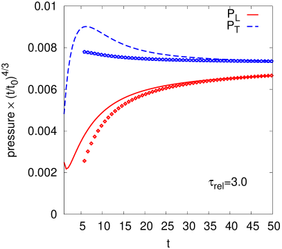
Figure 2: (Color online) Evolution of the energy density (left), and longitudinal and transverse pressures (right), obtained by solving the Boltzmann equation with the relaxation time approximation, Eq. (32), full lines. Both quantities are rescaled by a factor $t^{4/3}$ so that they approach constant values in the ideal hydrodynamical regime. The initial difference between the longitudinal and the transverse pressures is due to the parameter $\xi$ in the initial distribution function. The symbols represent the corresponding solutions of the Navier-Stokes hydrodynamics, started at time $t=50$ (in units of $Q_{s}^{-1}$) and evolved backwards in time.

The moments can be calculated from the distribution function given in Eq. (32). Consider first the free-streaming regime ($\tau_{\rm rel}\rightarrow\infty$). In this case, one has

$${\cal L}_{n}^{\mbox{\tiny FS}}=\frac{f_{0}Q_{s}^{4}}{4(2\pi)^{2}}\left(\frac{t_{0}}{\xi t}\right)\mathcal{F}_{n}\left(\frac{t_{0}}{\xi t}\right),$$ (34)

where $\mathcal{F}_{n}(x)$ is a function defined from the following integral ($0\leq x\leq 1$)

$$\mathcal{F}_{n}(x)=\int_{-1}^{1}dy\left[1-(1-x^{2})y^{2}\right]^{1/2}P_{2n}\left(\frac{xy}{\left[1-(1-x^{2})y^{2}\right]^{1/2}}\right)\,.$$ (35)

This function has the following limits: $\mathcal{F}_{n}(x)\to\pi P_{2n}(0)/2$ as $x\to 0$, and $\mathcal{F}_{n\neq 0}(x)\to 0$ as $x\to 1$. Thus, for asymptotically large $t$, $t\gg t_{0}/\xi$, $\mathcal{F}_{n}(x)$ reduces to a constant, and the moments decay as $1/t$. When $t=t_{0}/\xi$, the moments with $n\neq 0$ vanish, which implies in particular that they vanish at $t=t_{0}$ if there is no initial momentum anisotropy ($\xi=1$). The energy density is given by the zeroth moment, with $\mathcal{F}_{0}(0)=\pi/2$ and $\mathcal{F}_{0}(1)=2$. To within the slowly varying function $\mathcal{F}_{0}(t_{0}/\xi t)$, the energy density exhibits the expected behavior in $1/t$. It can also be verified that the longitudinal pressure drops rapidly, as $\sim 1/t^{2}$, so that at times $t\gg t_{0}/\xi$, the distribution function is peaked around $p_{z}=0$, and the energy density is dominated by transverse degrees of freedom.

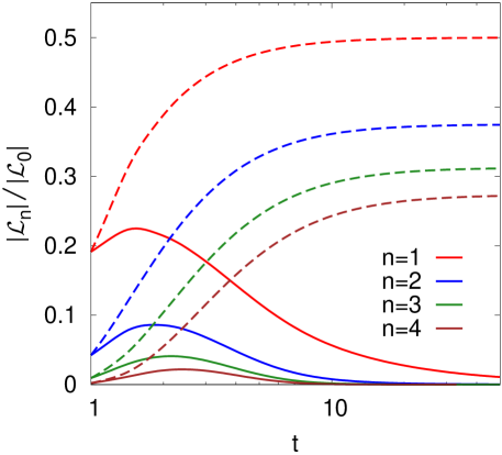
Figure 3: (Color online) Time evolution of the first few moments ($n=1,\cdots,4$, from top to bottom) normalized by the energy density, and obtained by solving the Boltzmann with the relaxation time approximation. The unit of time is $Q_{s}^{-1}$, and both the relaxation time $\tau_{\rm rel}$ and the initial time $t_{0}$ are set equal to $Q_{s}^{-1}$, i.e., $\tau_{\rm rel}=Q_{s}^{-1}=t_{0}$. The dashed lines are the corresponding moments for the free streaming solution, Eq. (34). We observe that by the time $t\gtrsim 15\tau_{\rm rel}$, all moments but ${\cal L}_{1}$ vanish.

For a finite $\tau_{\rm rel}$, Eq. (32) leads to

$${\cal L}_{n}(t)=\;e^{-(t-t_{0})/\tau_{\rm rel}}{\cal L}_{n}^{\mbox{\tiny FS}}+6\zeta(4)\int_{t_{0}}^{t}\frac{dt^{\prime}}{(2\pi)^{2}}\frac{e^{-(t-t^{\prime})/\tau_{\rm rel}}}{\tau_{\rm rel}}T(t^{\prime})^{4}\left(\frac{t^{\prime}}{t}\right)\mathcal{F}_{n}(t^{\prime}/t)\,,$$ (36)

where $\zeta(n)$ is the Riemann-zeta function. In this equation, the first term represents the contribution of the free-streaming of the initial distribution. This is suppressed in a time scale $\tau_{\rm rel}$, i.e., when collisions start to play a significant role. One thus expects the evolution of the moments to exhibit a transition between the free-streaming regime at short time, $t\ll\tau_{\rm rel}$, and the late time regime, dominated by collisions and represented by the second term in Eq. (36).

Figure 4: (Color online) Evolution of the moment ${\cal L}_{1}$ obtained from the solution of the Boltzmann equation in the relaxation time approximation, plotted in terms of the ratio $-t{\cal L}_{1}/2s$, with $s$ the entropy density. According to Eq. (23), this ratio can be identified, in the hydrodynamics regime and in leading order, to $\eta/s$. Three values of the relaxation time are considered $\tau_{\rm rel}=0.3,1,3$ (in units of $Q_{s}^{-1}$), with the same initial condition (Eq. (29)) in the three cases. The solid lines represent the analytical expression $\eta/s=\frac{1}{5}T\tau_{\rm rel}$ obtained in the (constant) relaxation time approximation, with the tempearture $T$ determined from Eq. (33). Note an unrealistic feature of this approximation which forces $\eta/s$ to vanish at large time. These curves confirm that viscous hydrodynamics can provide an accurate description for $t\gtrsim 15\,\tau_{\rm rel}$.

Figure 3 displays the evolution of the absolute values of the normalized moments $|{\cal L}_{n}/{\cal L}_{0}|$ up to $n=4$ (recall that ${\cal L}_{1}$ and ${\cal L}_{3}$ are negative). Also shown are the moments of the pure free-streaming solution, Eq. (34), which saturate at late times to their corresponding asymptotic values determined by $\mathcal{F}_{n}(0)$, namely,

$$\frac{|{\cal L}_{2n}^{\mbox{\tiny FS}}|}{|{\cal L}^{\mbox{\tiny FS}}_{0}|}\xrightarrow[]{t\gg t_{0}}\frac{(2n-1)!!}{(2n)!!}\,.$$ (37)

Note that this limit is independent of the initial pressure anisotropy paramater $\xi$. Clearly, the isotropization of the momentum distribution, signaled by the vanishing of the moments, can only be achieved by the collisions. Indeed the effect of the collisions starts to be visible around the time scale $(t-t_{0})\sim\tau_{\rm rel}$ where they begin to compete with the free streaming and later drive the momentum distribution to isotropy. Another effect of the collisions is to reduce the overall magnitude of the higher moments. As can be seen on Fig. 3, while the free streaming moments evolve towards comparable (within a factor 2) values at late times, the hierarchy of moments present in the initial condition is preserved but after a time $t\gtrsim 15\,\tau_{\rm rel}$ only the moment ${\cal L}_{1}$ remains significant. At this time the evolution of the system is well accounted for by viscous hydrodynamics.

This is confirmed by a more detailed study of the late-time evolution of the moments in Eq. (36). First we consider the moment ${\cal L}_{1}$. According to Eq. (23), the ratio between this moment and the entropy density, more precisely $-t{\cal L}_{1}/2s$, approaches $\eta/s$ in the hydrodynamic regime. This ratio is plotted in Fig. 4, where we purposely rescaled the time in Fig. 4 by $1/\tau_{\rm rel}$ so that they evolve on the same time scale. As time increases, $-t{\cal L}_{1}/2s$ indeed approaches the kinetic theory expectation: $\eta/s=\frac{1}{5}T\tau_{\rm rel}$, and reaches it for $t\gtrsim 15\,\tau_{\rm rel}$.

Figure 5 completes the discussion and illustrates the system evolution in terms of higher order moments. Again, we consider specified dimensionless combinations of moments which are supposed to reduce to dimensionless ratios of higher order transport coefficients at late times. The following combination

$$\frac{4{\cal L}_{2}\times{\cal L}_{0}}{{\cal L}_{1}^{2}}\rightarrow\frac{\lambda_{1}+\eta\tau_{\pi}}{\eta^{2}/(e+{\mathcal{P}})}$$ (38)

plotted in Fig. 5(a) is related to second order transport coefficients $\lambda_{1}$ and $\tau_{\pi}$. In a similar way, the combinations

$$\frac{8}{9}\frac{{\cal L}_{1}{\cal L}_{3}}{{\cal L}_{2}^{2}}\quad\mbox{and}\quad\frac{3}{4}\frac{{\cal L}_{2}{\cal L}_{4}}{{\cal L}_{3}^{2}}$$ (39)

that are plotted in Fig. 5(b) and (c), respectively, involve some 3rd order and 4th order transport coefficients.

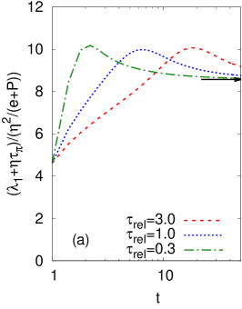
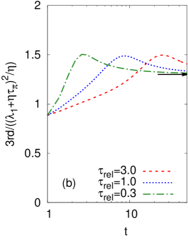
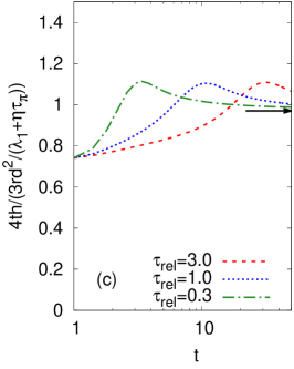
Figure 5: (Color online) Evolution of higher order moments, plotted in specified combinations which correspond to dimensionless ratios of transport coefficients in hydrodynamics regime. Black arrows indicate asymptotic values. Note that for $(\lambda_{1}+\eta\tau_{\pi})/(\eta^{2}/(e+{\mathcal{P}}))$, the asymptotic value is consistent with what was expected from kinetic theory York and Moore (2009).

Although these have not yet been determined in viscous hydrodynamics it is nevertheless interesting to estimate their ratios from the asymptotic behaviors: these are the black arrows in Fig. 5. Note that the asymptotic value of $(\lambda_{1}+\eta\tau_{\pi})/\eta^{2}/(e+{\mathcal{P}})\approx 8.57$ in Fig. 5(a) is consistent with what one expects from kinetic theory with a linear ansatz for the relaxation time York and Moore (2009). The asymptotic values of the ratios in Fig. 5(b) and (c) are found to be approximately 1.3 and 1.0, respectively.

Figure 6: Double ratios between transport coefficients, characterized in terms from $c_{n}$’s, for a conformal and classical gas. The results have been obtained analytically for the quadratic ansatz of the relaxation time (filled points) and numerically for the linear ansatz (open symbols).

Actually, the combinations plotted in Fig. 5 are nothing but double ratios among three consecutive orders of transport coefficients (to within simple numerical constants). In terms of the $c_{n}$’s defined in Eq. (27), these are

$$\frac{c_{n-1}c_{n+1}}{c_{n}^{2}}=\left(\frac{c_{n+1}}{c_{n}}\right)\bigg{/}\left(\frac{c_{n}}{c_{n-1}}\right)\,.$$ (40)

Asymptotic values of these double ratios can be obtained analytically in the case of the quadratic ansatz for the relaxation time (Eq. (28)), or numerically for the linear ansatz. Results for these two cases are shown in Fig. 6 for $n\leq 20$ and $n\leq 5$, respectively, as filled points and open symbols. For large $n$, the double ratio is seen to approach unity from above, which implies a saturation of transport coefficients of asymptotically high orders. This behavior reflects the fact that the gradient expansion leading to viscous hydrodynamics is only asymptotic Grad (1963); Groot et al. (1980) (see also Refs. Heller et al. (2016); Denicol and Noronha (2016) for a recent discussion of this issue within the context of Bjorken expansion).

III.2 Quark-gluon system with small angle approximation

We now apply the analysis of the previous section to the evolution of a quark-gluon plasma containing $N_{f}=N_{c}=3$ flavors of massless quarks, and introduce separate distributions for quarks ($f_{q}$) and gluons ($f_{g}$). We consider QCD tree-level 2 to 2 scatterings, within the small angle approximation. Following the strategy taken in Ref. Blaizot et al. (2014), we reduce the coupled Boltzmann equations for the gluon distribution function $f_{g}$ and the quark distribution $f_{q}$ to coupled Fokker-Plank equations,

$$\frac{\partial f_{g}}{\partial t}+{\bf v}\cdot\nabla_{\bf p}f_{g} =-\nabla_{\bf p}\cdot\mathcal{J}_{g}+\mathcal{S}_{g}\,,$$ (41a)

$$\frac{\partial f_{q}}{\partial t}+{\bf v}\cdot\nabla_{\bf p}f_{q} =-\nabla_{\bf p}\cdot\mathcal{J}_{q}+\mathcal{S}_{q}\,,$$ (41b)

where the currents $\mathcal{J}_{q,g}$ and sources $\mathcal{S}_{q,g}$ are given by

$$\mathcal{J}_{g}= -(4\pi\alpha_{s}^{2}\ell)N_{c}\left[{\mathcal{I}}_{a}\nabla_{\bf p}f_{g}+{\mathcal{I}}_{b}\frac{{\bf p}}{p}f_{g}(1+f_{g})\right]\,,$$ (42a)

$$\mathcal{J}_{q}= -(4\pi\alpha_{s}^{2}\ell)C_{F}\left[{\mathcal{I}}_{a}\nabla_{\bf p}f_{q}+{\mathcal{I}}_{b}\frac{{\bf p}}{p}f_{q}(1-f_{q})\right]\,,$$ (42b)

$${\mathcal{S}}_{g}= -\frac{N_{f}}{C_{F}}{\mathcal{S}}_{q}=\frac{(4\pi\alpha_{s}^{2}\ell)C_{F}N_{f}{\mathcal{I}}_{c}}{p}\left[f_{q}(1+f_{g})-f_{g}(1-f_{q})\right]\,.$$ (42c)

While the currents are associated to conservation laws (the particle numbers), and hence to elastic processes, the sources arise from the inelastic processes that correspond to quark creations and annihilations. Note that all the processes considered conserve the total number of particles. The quantities ${\mathcal{I}}_{a}$, ${\mathcal{I}}_{b}$ and ${\mathcal{I}}_{c}$ are the following integrals,

$${\mathcal{I}}_{a} =\int_{p}p^{0}[N_{c}f_{g}(1+f_{g})+N_{f}f_{q}(1-f_{q})],$$ (43a)

$${\mathcal{I}}_{b} =\int_{p}\frac{2p^{0}}{p}(N_{c}f_{g}+N_{f}f_{q}),$$ (43b)

$${\mathcal{I}}_{c} =\int_{p}\frac{p^{0}}{p}(f_{g}+f_{q}).$$ (43c)

For a thermal system in equilibrium, ${\mathcal{I}}_{a}/{\mathcal{I}}_{b}$ is identical to the temperature. Finally the quantity $\ell$ denotes a logarithmically divergent integral (the Coulomb logarithm)

$$\ell=\int_{q_{min}}^{q_{max}}\frac{dq}{q},$$ (44)

which arises from small angle scatterings. For a QCD plasma close to thermal equilibrium, $\ell\approx\mbox{ln}g^{-1}$ (with $g$ the strong coupling constant). This Coulomb logarithm is treated as a constant in the present work.

With all the quantities thus specified, one may check that the collision kernel in Eq. (41) conserves energy-momentum and constituent number (number of gluons, quarks and anti-quarks), which implies that the local equilibrium distribution is, in the local rest frame, a Bose-Einstein distribution for the gluons and a Fermi-Dirac distribution for the quarks and the antiquarks, with given temperature and chemical potential (see Ref. Blaizot et al. (2014) for details).

Assuming Bjorken flow, and integrating over azimuthal angle, one transforms Eq. (41) into

$$\partial_{t}f_{g}-\frac{p^{z}}{t}\partial_{p^{z}}f_{g}= \frac{1}{p_{T}}\frac{\partial}{\partial p_{T}}(p_{T}J_{g}^{T})+\frac{\partial}{\partial p^{z}}J_{g}^{z}+S_{g}\,,$$ (45a)

$$\partial_{t}f_{q}-\frac{p^{z}}{t}\partial_{p^{z}}f_{q}= \frac{1}{p_{T}}\frac{\partial}{\partial p_{T}}(p_{T}J_{q}^{T})+\frac{\partial}{\partial p^{z}}J_{q}^{z}+S_{q}\,,$$ (45b)

where $J_{g}$, $J_{q}$, $S_{g}$ and $S_{q}$ are the currents and sources obtained from Eqs. (42) after a simple rescaling that eliminates the common factor $4\pi\alpha_{s}^{2}{\ell}$. That is, in deriving Eq. (45) we have absorbed the factor $\alpha_{s}^{2}\ell$ in a redefinition of the time, $t\rightarrow t(\alpha_{s}^{2}\ell)$, and we have redefined the integrals (43) by multiplying them by a factor $4\pi$. With these redefinitions, the time scale of the simulation is measured in units of $\tau_{s}\equiv(\alpha_{s}^{2}\ell Q_{s})^{-1}$. For technical reasons related to the numerical precision of the calculated moments, our simulations end at $t=400\tau_{s}$.

We initialize the system at a time $t_{0}=1/Q_{s}$, and assume that, at this time, the system contains only gluons, with a distribution function given by Eq. (29). In order to be able to compare with the previous subsection, we shall make a rough estimate of the relaxation time. To do so, we focus on the gluon sector, and the diffusion piece of the current (the one proportional to the gradient of the distribution). By writing the linearized version of the gluon kinetic equation (Eq. (41)) as $\delta f_{g}/\tau_{\rm rel}\sim\delta f_{g}/p^{2}$, we get

$$\frac{1}{\tau_{\rm rel}}\sim 4\pi\alpha_{s}^{2}\ell N_{c}^{2}\frac{f_{0}}{p^{2}}\frac{Q_{s}^{3}}{6\pi^{2}}.$$ (46)

For $p\approx Q_{s}$, $N_{c}=3$, this yields

$$\frac{1}{\tau_{\rm rel}}\sim\frac{1}{\tau_{s}}\frac{6f_{0}}{\pi}\sim 0.2\quad\mbox{and}\quad\tau_{\rm rel}\sim 5\tau_{s}.$$ (47)

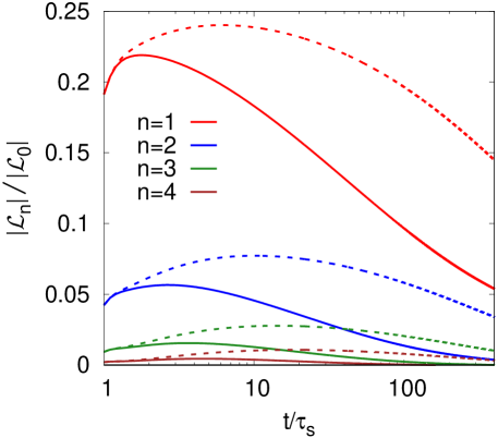
Figure 7: (Color online) Time evolution of absolute values of the moments ${\cal L}_{n}$ normalized by the energy density ${\cal L}_{0}$, for a pure gluon system (solid lines) and a quark gluon plasma (dashed lines), as obtained from solving the Boltzmann equation within the small scattering angle approximation.

We first plot in Fig. 7 the absolute values of the moments ${\cal L}_{n}$ divided by the energy density, for $n=1$ up to $n=4$ for a pure gluon system (solid lines) and a QGP (dashed lines). The pattern seen here is analogous to that in Fig. 3 corresponding to the relaxation time approximation. The curves present a (broad) peak at the transition between free-streaming at early times and a collision dominated regime at late times. Clearly, the elastic collisions, treated in the small angle approximation, isotropize the system: all moments tend to vanish in the collision dominated regime. The higher moments are damped on a time scale that decreases with increasing order of the moment. Overall, the evolution of moments in Fig. 7 is comparable to that in Fig. 3, even semi-quantitatively (to within a factor $\sim 2$) if one takes into account the crude estimate of the relaxation time presented above. Note that for a quark-gluon plasma, the isotropization process is significantly delayed and the transition from the free-streaming regime to the collision dominated regime is slower than for the pure gluon case.

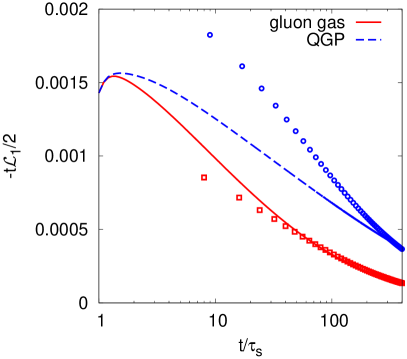
Figure 8: (Color online) Evolution of the moment ${\cal L}_{1}$ obtained by solving the Boltzmann equation for a pure gluon gas (full lines) and a quark-gluon plasma (dashed line). These are compared to the viscous hydrodynamical evolution (symbols), where the initial conditions are fixed at the latest time, $t=400\,\tau_{s}$.

In order to compare with hydrodynamics we need to take into account the fact that our Boltzmann equation conserves the number of constituents. The equation for the energy density needs therefore to be completed by a continuity equation for the number density, which, for Bjorken flow, has the simple solution $n(t)=n(t_{0})t_{0}/t$. This also implies that the local distribution function depends on a temperature and a chemical potential. Details on the hydrodynamical calculations are given in Appendix B.

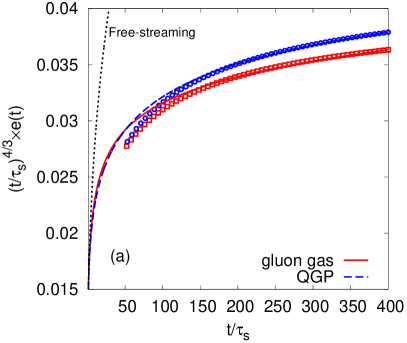
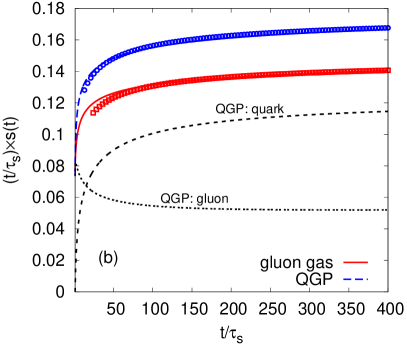
Figure 9: (Color online) Left (a): Evolution of the energy density (rescaled by $t^{4/3}$) of a pure gluon system (red solid line) and a QGP (blue dashed line) as obtained by solving the Boltzmann equation within the small scattering angle approximation, Eqs. (45). Right (b): Evolution of entropy density of a pure gluon gas (red) and of a QGP (blue). The blue dashed and dotted lines correspond to the gluon and quark components of a QGP respectively. The symbols in both (a) and (b) represent the corresponding solutions of from Navier-Stokes equations, as described in the text.

The fact that particle number is conserved can modify the shear viscosity from its value at vanishing chemical potential. When $\mu=0$, it is known in weak coupling QCD Baym et al. (1990); Arnold et al. (2000) that

$$\eta(T,0)=\kappa\frac{T^{3}}{\alpha_{s}^{2}\ell}\,,$$ (48)

where $\kappa$ is a constant depending on the number of colors and quark flavors. For instance, for a pure gluon system, $\kappa\approx 0.17$. We do not have (yet) a precise determination of the viscosity appropriate to the present setting. In the present work, we shall therefore rely on a crude approximation whereby we use Eq. (48) for $\eta$, with $\kappa$ left as an adjustable parameter.

We initialize the hydrodynamical calculation at $t=400\tau_{s}$, which corresponds to the largest time for which we can solve accurately the Boltzmann equation. At that time, the energy density and the number density are identified with those values obtained from the solution of the Boltzmann equation. Since after $t=200\tau_{s}$, the high order ($n\geq 2$) moments are relatively less significant, as shown in Fig. 7, one expects the system evolution to follow first order viscous hydrodynamics at later times, $t\gtrsim 200\tau_{\rm s}$. Note that the ratio ${\mathcal{P}}_{L}/{\mathcal{P}}_{T}\approx 0.85$ and $0.62$ at $t=400\tau_{s}$ for the pure gluon gas and the QGP, respectively. This value for the pure glue system (0.85) is to be compared with that obtained in the previous subsection in the relaxation time approximation (0.9), at times where we found the system to be in the (viscous) hydrodynamic regime. The evolution of the moment ${\cal L}_{1}$ is shown in Fig. 8, and compared to the solution of the Navier-Stokes hydrodynamics. This comparison allows for the determination of the parameter $\kappa$ in Eq. (48). We obtain $\kappa=0.62$ and $0.67$ respectively for the pure gluon gas and the QGP. These values are about four times larger than the values expected from weak coupling estimates. These estimates, however, do not take into account the effect of a non vanishing chemical potential, and the formula (48) is from that point of view only an approximation in the present context, as already stated. This approximation is sufficient for our purpose: with the viscosity given by Eq. (48) the pattern observed in Fig. 8 is similar to that observed in Fig. 4, showing a brief free-streaming at early times, followed by a slow approach to the viscous hydrodynamic regime at late times.

The evolution of the energy density obtained from the solutions of Eqs. (41) is presented in Fig. 9 (a) for a pure gluon gas (red solid line) and a QGP (blue dashed line). The energy density is rescaled by a factor $t^{4/3}$ to be plotted on a visible scale, and also to make clearer the approach to ideal hydrodynamics where the quantity should be constant. One sees that this ideal regime is not reached at $t=400\,\tau_{s}$, which was also indicated by the non zero value of ${\cal L}_{1}$ at that time (see Fig. 4).

Figure 9 (b) displays the evolution of the entropy density in the transverse plane. It goes to a constant when the ideal hydrodynamical regime is reached. As expected in kinetics, a significant amount of entropy is produced at early times, when the system starts to re-distribute momenta from the initial step function toward a smoother distribution, with in particular a rapid growth of soft modes Blaizot et al. (2013, 2014). More entropy is generated in the QGP (blue line), as compared to the pure gluon gas (red line), due to the additional quark degrees of freedom which, for three flavors, contribute about twice as much as the gluons to the total entropy (chemical equilibrium is nearly reached at $t=400\tau_{\rm s}$). One sees that Navier-Stokes hydrodynamics describes well the entropy production already at times $t\gtrsim 100\tau_{s}$, for both the gluon gas and the QGP.

IV Summary and conclusions

In this paper, we have proposed a set of moments, ${\cal L}_{n}$, that provide a simple characterization of the momentum anisotropy of the momentum distribution function and take into account Bjorken’s symmetry of the longitudinally expanding quark-gluon plasmas created in relativistic heavy ion collisions. At late times, i.e., when the hydrodynamic regime is approached, these moments can be associated to viscous corrections to the energy-momentum tensor, order-by-order in a gradient expansion. The explicit correspondence with the transport coefficients of viscous conformal hydrodynamics has been established. The generalizations to cases without conformal symmetry can be carried out in a similar way. These moments offer a convenient tool to characterize the onset of hydrodynamics.

The time evolution of the moments was studied first with the help of a Boltzmann equation solved within a (constant) relaxation time approximation. This has allowed us to verify the correspondence of the ${\cal L}_{n}$’s with viscous hydrodynamics up to order $n=4$. The onset of hydrodynamics was subsequently analyzed in terms of these ${\cal L}_{n}$’s up to $n=4$. The approach to hydrodynamics manifests itself as the decrease of the magnitudes of the ${\cal L}_{n}$ with $n$ larger than 1. In fact the moments ${\cal L}_{n}$ are damped more and more rapidly as $n$ increases, which reflects the fact that long wavelength modes thermalize faster than short wavelength ones. Note that the preeminence of the moment ${\cal L}_{1}$ is reminiscent of the arguments used in anisotropic hydrodynamics Martinez and Strickland (2010); Florkowski and Ryblewski (2011).

Similar patterns are observed when we use the more realistic $2\leftrightarrow 2$ QCD matrix elements in the Boltzmann equation, which we have solved numerically, within the small scattering angle approximation. Again, we have determined the evolution of ${\cal L}_{n}$ up to order $n=4$. In the calculations that we have presented, quarks are entirely generated via gluon-quark conversion according to tree-level QCD processes. Although quarks are produced on a relatively short time scale, this production is hindered by Pauli blocking effects which tend to delay significantly the thermalization and the onset of hydrodynamics. Finally, the present analysis ignores the inelastic collisions (soft and collinear splitting of gluons) whose role in the isotropization is emphasized in particular in the bottom-up scenario. We defer their study to future work.

Appendix A Contraction of irreducible tensors and Legendre polynomials

The equation (19) expresses in terms of a Legendre polynomial the tensorial structure that appears in the leading order gradient expansion of the distribution function. This can be generalized to higher orders. In particular, in the $n$-th order viscous corrections, the term with the highest power in momentum involves the contractions of irreducible tensors of rank $2n$.

Generally, the contraction of a two irreducible tensor of rank $2n$ constructed from the product of $2n$ vectors $A^{\mu}$ and $2n$ vectors $B_{\mu}$ can be written in terms of Legendre polynomials as follows (cf. Hess (2015)),

$${\langle}A^{\mu_{1}}A^{\mu_{2}}\ldots A^{\mu_{2n}}\rangle{\langle}B_{\mu_{1}}B_{\mu_{2}}\ldots B_{\mu_{2n}}\rangle=|A|^{2n}|B|^{2n}N_{2n}P_{2n}(\hat{A}\cdot\hat{B})\,.$$ (49)

In this equation, $|A|$ and $|B|$ denote the modulus of the vectors, while $\hat{A}$ and $\hat{B}$ are unit vectors. The constant coefficient is

$$N_{2n}=\frac{(2n)!}{(4n-1)!!}\,.$$ (50)

As a check, let us apply Eq. (49) to $P^{\mu}P^{\nu}\sigma_{\mu\nu}$. First, we note the following identity,

$$P^{\mu}P^{\nu}\sigma_{\mu\nu}\equiv 2P^{\mu}P^{\nu}\langle\nabla_{\mu}U_{\nu}\rangle=2\langle P^{\mu}P^{\nu}\rangle\nabla_{\mu}U_{\nu}=2\langle P^{\mu}P^{\nu}\rangle\langle\nabla_{\mu}U_{\nu}\rangle\,.$$ (51)

We also know that the tensor $\nabla_{\mu}U_{\nu}$ with respect to Bjorken flow has only non-zero component at $\eta\eta$ as $\nabla_{\eta}U_{\eta}=\tau$, it is thus able to write equivalently

$$\nabla_{\mu}U_{\nu}=R_{\mu}R_{\nu}\,,$$ (52)

with $R_{\mu}=(0,0,0,\sqrt{\tau})$ as a 4-vector. Combining Eqs. (49) to (52) and making a coordinate transformation from $p^{\eta}$ to $p^{z}$, one gets immediately Eq. (19)

$$P^{\mu}P^{\nu}\sigma_{\mu\nu}\equiv\frac{2p^{2}}{\tau}\times\frac{2}{3}\times P_{2}(\cos\theta)\,.$$ (53)

The similar procedure can be applied to the contraction of the irreducible tensor of rank $2n$ of Eq. (26). We get

$$P^{\mu_{1}}P^{\mu_{2}}\ldots P^{\mu_{2n}}\langle\sigma_{\mu_{1}\mu_{2}}\ldots\sigma_{\mu_{2n-1}\mu_{2n}}\rangle= 2^{n}\langle P^{\mu_{1}}P^{\mu_{2}}\ldots P^{\mu_{2n}}\rangle\langle\nabla_{\mu_{1}}U_{\mu_{2}}\ldots\nabla_{\mu_{2n-1}}U_{\mu_{2n}}\rangle$$

$$= 2^{n}\langle P^{\mu_{1}}P^{\mu_{2}}\ldots P^{\mu_{2n}}\rangle\langle R_{\mu_{1}}R_{\mu_{2}}\ldots R_{\mu_{2n}}\rangle$$

$$= 2^{n}\frac{p^{2n}}{\tau^{n}}N_{2n}P_{2n}(\cos\theta)\,.$$ (54)

Appendix B Hydrodynamics with a with non-zero chemical potential

When comparing the solution of the Boltzmann equation in Section III.2 to viscous hydrodynamics, we need to pay attention to the fact that the QCD 2-to-2 scatterings conserve the number of constituents. As a result the hydrodynamic equations should be complemented with a continuity equation, i.e., we need to solve

$$\partial_{\mu}T^{\mu\nu}=0\,,\qquad\partial_{\mu}n^{\mu}=0\,,$$

with energy-momentum tensor $T^{\mu\nu}$ given in Eq. (11) and

$$n^{\mu}=nU^{\mu}+I^{\mu}\,.$$ (55)

Here, $I^{\mu}$ represents a viscous correction to the conserved number current. For Bjorken flow, this correction vanishes and, up to first order in the viscous corrections, the hydrodynamic equations reduce then to

$$\partial_{\tau}e+\frac{e+{\mathcal{P}}}{\tau}=\frac{4\eta(T,\mu)}{3\tau^{2}}\,,$$ (56a)

$$\partial_{\tau}n+\frac{n}{\tau}=0\,.$$ (56b)

These equations are complemented by the equation of state for massless particles, ${\cal P}=e/3\sim T^{4}$. Furthermore the density and the energy density are related to the temperature and the chemical potential by (for gluons)

$$n(T,\mu)= 2(N_{c}^{2}-1)\int_{p}\frac{p}{\exp(p/T-\mu/T)-1}\,,$$ (57a)

$$e(T,\mu)= 2(N_{c}^{2}-1)\int_{p}\frac{p^{2}}{\exp(p/T-\mu/T)-1}\,,$$ (57b)

(with analogous formulae for quarks and antiquarks). Note that the values of the temperature and chemical potential thus determined are not too different from those obtained by a fit of the distribution function calculated from the kinetic equation. The second equation (56) can be solved independently and yields $\tau n(\tau)={\rm cste}$. The equation for the energy density requires the knowledge of $\eta(T,\mu)$. In this work we ignore the explicit dependence of $\eta$ on the chemical potential, and use simply Eq. (48) for $\eta$, with $\kappa$ an adjustable parameter. The comparison with hydrodynamics is done by fixing “initial” conditions at $t=400\tau_{s}$, and running the equations backwards in time. That is, the initial density and energy density allow us to determine the initial temperature and chemical potential, and hence the viscosity. This process can be repeated to evolve backwards in times steps. The entropy is determined from the thermodynamic relation $Ts=e+{\mathcal{P}}-\mu n$, which does not involve explicitly the viscosity. This provides a check of the overall consistency of the calculation.

References

- Heinz and Snellings (2013) Ulrich Heinz and Raimond Snellings, “Collective flow and viscosity in relativistic heavy-ion collisions,” Ann. Rev. Nucl. Part. Sci. 63, 123–151 (2013), arXiv:1301.2826 [nucl-th] .
- Epelbaum and Gelis (2013) Thomas Epelbaum and Francois Gelis, “Pressure isotropization in high energy heavy ion collisions,” Phys. Rev. Lett. 111, 232301 (2013), arXiv:1307.2214 [hep-ph] .
- Berges et al. (2014) Juergen Berges, Kirill Boguslavski, Soeren Schlichting, and Raju Venugopalan, “Universal attractor in a highly occupied non-Abelian plasma,” Phys. Rev. D89, 114007 (2014), arXiv:1311.3005 [hep-ph] .
- Mueller and Son (2004) A. H. Mueller and D. T. Son, “On the Equivalence between the Boltzmann equation and classical field theory at large occupation numbers,” Phys. Lett. B582, 279–287 (2004), arXiv:hep-ph/0212198 [hep-ph] .
- Kurkela and Moore (2011) Aleksi Kurkela and Guy D. Moore, “Thermalization in Weakly Coupled Nonabelian Plasmas,” JHEP 12, 044 (2011), arXiv:1107.5050 [hep-ph] .
- Kurkela and Lu (2014) Aleksi Kurkela and Egang Lu, “Approach to Equilibrium in Weakly Coupled Non-Abelian Plasmas,” Phys. Rev. Lett. 113, 182301 (2014), arXiv:1405.6318 [hep-ph] .
- Blaizot et al. (2013) Jean-Paul Blaizot, Jinfeng Liao, and Larry McLerran, “Gluon Transport Equation in the Small Angle Approximation and the Onset of Bose-Einstein Condensation,” Nucl. Phys. A920, 58–77 (2013), arXiv:1305.2119 [hep-ph] .
- Blaizot et al. (2014) Jean-Paul Blaizot, Bin Wu, and Li Yan, “Quark production, Bose–Einstein condensates and thermalization of the quark–gluon plasma,” Nucl. Phys. A930, 139–162 (2014), arXiv:1402.5049 [hep-ph] .
- Xu et al. (2015) Zhe Xu, Kai Zhou, Pengfei Zhuang, and Carsten Greiner, “Thermalization of gluons with Bose-Einstein condensation,” Phys. Rev. Lett. 114, 182301 (2015), arXiv:1410.5616 [hep-ph] .
- Kurkela and Zhu (2015) Aleksi Kurkela and Yan Zhu, “Isotropization and hydrodynamization in weakly coupled heavy-ion collisions,” Phys. Rev. Lett. 115, 182301 (2015), arXiv:1506.06647 [hep-ph] .
- Keegan et al. (2016) Liam Keegan, Aleksi Kurkela, Paul Romatschke, Wilke van der Schee, and Yan Zhu, “Weak and strong coupling equilibration in nonabelian gauge theories,” JHEP 04, 031 (2016), arXiv:1512.05347 [hep-th] .
- Bazow et al. (2016) D. Bazow, G. S. Denicol, U. Heinz, M. Martinez, and J. Noronha, “Nonlinear dynamics from the relativistic Boltzmann equation in the Friedmann-Lemaître-Robertson-Walker spacetime,” (2016), arXiv:1607.05245 [hep-ph] .
- Baier et al. (2008) Rudolf Baier, Paul Romatschke, Dam Thanh Son, Andrei O. Starinets, and Mikhail A. Stephanov, “Relativistic viscous hydrodynamics, conformal invariance, and holography,” JHEP 04, 100 (2008), arXiv:0712.2451 [hep-th] .
- Bjorken (1983) J. D. Bjorken, “Highly Relativistic Nucleus-Nucleus Collisions: The Central Rapidity Region,” Phys. Rev. D27, 140–151 (1983).
- Baier et al. (2001) R. Baier, Alfred H. Mueller, D. Schiff, and D. T. Son, “’Bottom up’ thermalization in heavy ion collisions,” Phys. Lett. B502, 51–58 (2001), arXiv:hep-ph/0009237 [hep-ph] .
- Tanji and Venugopalan (2017) Naoto Tanji and Raju Venugopalan, “Effective kinetic description of the expanding overoccupied Glasma,” Phys. Rev. D95, 094009 (2017), arXiv:1703.01372 [hep-ph] .
- Heller et al. (2012) Michal P. Heller, Romuald A. Janik, and Przemyslaw Witaszczyk, “The characteristics of thermalization of boost-invariant plasma from holography,” Phys. Rev. Lett. 108, 201602 (2012), arXiv:1103.3452 [hep-th] .
- Teaney and Yan (2014) Derek Teaney and Li Yan, “Second order viscous corrections to the harmonic spectrum in heavy ion collisions,” Phys. Rev. C89, 014901 (2014), arXiv:1304.3753 [nucl-th] .
- Yan (2012) Li Yan, “Anisotropic Flow and Viscous Hydrodynamics,” Proceedings, 28th Winter Workshop on Nuclear Dynamics (WWND 2012): Dorado del Mar, Puerto Rico, April 7-14, 2012, J. Phys. Conf. Ser. 389, 012014 (2012), arXiv:1208.3011 [nucl-th] .
- Dusling et al. (2010) Kevin Dusling, Guy D. Moore, and Derek Teaney, “Radiative energy loss and v(2) spectra for viscous hydrodynamics,” Phys. Rev. C81, 034907 (2010), arXiv:0909.0754 [nucl-th] .
- Gelis et al. (2010) Francois Gelis, Edmond Iancu, Jamal Jalilian-Marian, and Raju Venugopalan, “The Color Glass Condensate,” Ann. Rev. Nucl. Part. Sci. 60, 463–489 (2010), arXiv:1002.0333 [hep-ph] .
- Arnold et al. (2006) Peter Brockway Arnold, Caglar Dogan, and Guy D. Moore, “The Bulk Viscosity of High-Temperature QCD,” Phys. Rev. D74, 085021 (2006), arXiv:hep-ph/0608012 [hep-ph] .
- Blaizot et al. (2017) Jean-Paul Blaizot, Jinfeng Liao, and Yacine Mehtar-Tani, “The thermalization of soft modes in non-expanding isotropic quark gluon plasmas,” Nucl. Phys. A961, 37–67 (2017), arXiv:1609.02580 [hep-ph] .
- Baym (1984) G. Baym, “THERMAL EQUILIBRATION IN ULTRARELATIVISTIC HEAVY ION COLLISIONS,” Phys. Lett. B138, 18–22 (1984).
- Florkowski and Ryblewski (2016) Wojciech Florkowski and Radoslaw Ryblewski, “Separation of elastic and inelastic processes in the relaxation-time approximation for the collision integral,” Phys. Rev. C93, 064903 (2016), arXiv:1603.01704 [nucl-th] .
- York and Moore (2009) Mark Abraao York and Guy D. Moore, “Second order hydrodynamic coefficients from kinetic theory,” Phys. Rev. D79, 054011 (2009), arXiv:0811.0729 [hep-ph] .
- Jaiswal (2013) Amaresh Jaiswal, “Relativistic third-order dissipative fluid dynamics from kinetic theory,” Phys. Rev. C88, 021903 (2013), arXiv:1305.3480 [nucl-th] .
- Grozdanov and Kaplis (2016) Sašo Grozdanov and Nikolaos Kaplis, “Constructing higher-order hydrodynamics: The third order,” Phys. Rev. D93, 066012 (2016), arXiv:1507.02461 [hep-th] .
- Grad (1963) Harold Grad, “Asymptotic theory of the boltzmann equation,” The Physics of Fluids 6, 147–181 (1963), http://aip.scitation.org/doi/pdf/10.1063/1.1706716 .
- Groot et al. (1980) S.R. Groot, W.A. Leeuwen, and C.G. van Weert, Relativistic kinetic theory: principles and applications (North-Holland Pub. Co., 1980).
- Heller et al. (2016) Michal P. Heller, Aleksi Kurkela, and Michal Spalinski, “Hydrodynamization and transient modes of expanding plasma in kinetic theory,” (2016), arXiv:1609.04803 [nucl-th] .
- Denicol and Noronha (2016) Gabriel S. Denicol and Jorge Noronha, “Divergence of the Chapman-Enskog expansion in relativistic kinetic theory,” (2016), arXiv:1608.07869 [nucl-th] .
- Baym et al. (1990) G. Baym, H. Monien, C. J. Pethick, and D. G. Ravenhall, “Transverse Interactions and Transport in Relativistic Quark - Gluon and Electromagnetic Plasmas,” Phys. Rev. Lett. 64, 1867–1870 (1990).
- Arnold et al. (2000) Peter Brockway Arnold, Guy D. Moore, and Laurence G. Yaffe, “Transport coefficients in high temperature gauge theories. 1. Leading log results,” JHEP 11, 001 (2000), arXiv:hep-ph/0010177 [hep-ph] .
- Martinez and Strickland (2010) Mauricio Martinez and Michael Strickland, “Dissipative Dynamics of Highly Anisotropic Systems,” Nucl. Phys. A848, 183–197 (2010), arXiv:1007.0889 [nucl-th] .
- Florkowski and Ryblewski (2011) Wojciech Florkowski and Radoslaw Ryblewski, “Highly-anisotropic and strongly-dissipative hydrodynamics for early stages of relativistic heavy-ion collisions,” Phys. Rev. C83, 034907 (2011), arXiv:1007.0130 [nucl-th] .
- Hess (2015) Siegfried Hess, Tensors for physics, Undergraduate Lecture Notes in Physics (Springer, Cham, 2015).