Optomechanical Toy Model for Gravitationally Induced Decoherence: Exact Solution

Abstract

I present the exact solution of a toy model for gravitationally induced decoherence. The toy model has Hamiltonian resembling optomechanical systems. It is an oscillator system coupled through its energy to an oscillator heat bath. I find the decoherence effect of vacuum fluctuations at zero temperature. Also for a finite bath I show that the decoherence is in general present and the system does not return to its initial coherence unless the fundamental frequencies of the bath have rational ratios.

The decoherence effect of gravitational perturbations has been studied by various authors by use of Born-Markov approximation Blencowe2013 . While the approximation is valid in certain limits it fails for zero temperature Blencowe2014pc . In this paper, we solve the toy model proposed by Blencowe as an illustrative example which may shed some lights on the gravity problemBlencowe2013 ; Blencowe2014pc . We solve the problem almost exactly without any use of Born-Markov approximation.

Since the toy model resembles genuine models of optomechanics Aspelmeyer2014 and variation of that may be used in quantum optics and cavity QED, we pay extra attention to finite bath. We show that in a finite bath the decoherence still takes place unless the fundamental frequencies of the bath ratios equal to rational numbers.

The toy model of Ref Blencowe2013 is an oscillator system with frequency $\omega_{0}$ coupled via its energy to an oscillator heat bath,

$$H=\hbar\omega_{0}a^{\dagger}a+\hbar\omega_{0}a^{\dagger}a\sum_{i}\lambda_{i}\frac{q_{i}}{\Delta_{i}}+\sum_{i}\left(\frac{p_{i}^{2}}{2m_{i}}+\frac{1}{2}m_{i}\omega_{i}^{2}q_{i}^{2}\right)$$ (1)

where $\Delta_{i}=\sqrt{\hbar/(2m_{i}\omega_{i})}$ is the ith bath oscillator’s zero-point uncertainty. In following we denote the Hamiltonian of the system by $H_{S}=\hbar\omega_{0}a^{\dagger}a$ and for convenience choose units in such a way that $\hbar=1$. We also write the total Hamiltonian in terms of annihilation and creation operators of the bath oscillators and drop the c-number vacuum energy of the bath, $\sum_{i}\frac{\hbar\omega_{i}}{2}$, as follows

$$H=H_{S}+H_{S}\sum_{i}\lambda_{i}(a^{\dagger}_{i}+a_{i})+\sum_{i}\omega_{i}a_{i}^{\dagger}a_{i}$$ (2)

As pointed out in Halataei2017d the vacuum energy of the bath does not appear in the original construction of the oscillator heat bath model by Caldeira and Leggett (App. C of Caldeira83 ). So it is more accurate not to include that term in the Hamiltonian and the density matrix of the bath in thermal equilibrium.

The universe $U$ (which is composed of the system plus the bath) is initially decoupled with total density matrix

$$\hat{\rho}_{U}(0)=\hat{\rho}_{S}(0)\otimes\hat{\rho}_{B}$$ (3)

where $\rho_{S}(0)$ is the initial density matrix of the system and the bath is in thermal equilibrium with density matrix

$$\hat{\rho}_{B}=\bigotimes_{i}\hat{\rho}_{B_{i}}=\bigotimes_{i}\frac{e^{-\omega_{i}a_{i}^{\dagger}a_{i}/k_{B}T}}{Z_{i}}$$ (4)

where the partition function of the ith oscillator of the bath is $Z_{i}=Tr_{B_{i}}\{e^{-\omega_{i}a_{i}^{\dagger}a_{i}/k_{B}T}\}$. As the universe evolves by time it entangles the system and the bath. The density matrix of the universe $\rho(t)$ in no longer a direct product of the that of the system and the heat bath. One has to calculate the reduced density matrix $\rho_{S}(t)$ as follows to obtain information about the system

$$\hat{\rho}_{S}(t)=\text{Tr}_{B}\hat{\rho}_{U}(t)$$ (5)

The question is how the off diagonal elements of the reduced density matrix of the system $\rho_{S}(t)$ decay in time ?

Without resort the Bron-Markov approximation, this problem is solved by Schlosshauer in Ref. Schlosshauer2007 for a single spin-$1/2$ particle in interaction with an oscillator heat bath. In Schlosshauer2007 the total Hamiltonian is similar to (2) and the Hamiltonian of the system $H_{S}\propto\sigma_{z}$ describes a spin-$1/2$ particle in magnetic field along the z axis.

We follow Schlosshauer scheme below and adapt it for the oscillator system. In addition we introduce a lower cut off frequency for the bath modes and study its effect, as this can appear in a gravitational problem. As for a finite heat bath and the false decoherence effect we make, however, a different comment than that given by Ref. Schlosshauer2007 (see below).

The Hamiltonian (2) consists of three parts, the system Hamiltonian $H_{S}$, the interaction Hamiltonian $H_{int}=H_{S}\sum_{i}\lambda_{i}(a_{i}^{\dagger}+a_{i})$ and the bath Hamiltonian $H_{B}=\sum_{i}\omega_{i}a_{i}^{\dagger}a_{i}$,

$$H=H_{S}+H_{int}+H_{B}.$$ (6)

Since the decaying behavior of the reduced density matrix is of interest here (and not its oscillatory one) we go to the interaction picture and solve the problem there. In this picture the interaction Hamiltonian $H_{int}(t)$ evolves as

$$H_{int}(t) = e^{i(H_{S}+H_{B})t}H_{int}e^{-i(H_{S}+H_{B})t}$$ (7)

$$= H_{S}\sum_{i}\lambda_{i}(a_{i}^{\dagger}e^{i\omega_{i}t}+a_{i}e^{-i\omega_{i}t})$$ (8)

From this one can construct the evolution operator in the interaction picture,

$$\hat{U}(t)=\mathcal{T}e^{-i\int_{0}^{\infty}dt^{\prime}H_{int}(t^{\prime})}$$ (9)

where $\mathcal{T}$ denotes the time ordered product. Since the commutator of the interaction Hamiltonian for two different times is a c-number,

$$[H_{int}(t),H_{int}(t^{\prime})]=-2i\sum_{i}\lambda_{i}^{2}\sin\omega_{i}(t-t^{\prime}),$$ (10)

one can write $U(t)$ as

$$\hat{U}(t)=e^{i\phi(t)}\exp\left[-i\int_{0}^{t}dt^{\prime}H_{int}(t^{\prime})\right]\equiv e^{i\phi(t)}\hat{V}(t)$$ (11)

where $\phi(t)$ is a global time dependent phase factor and there is no time ordering above Schlosshauer2007 . Taking the integral one finds

$$\hat{V}(t)=\exp\left[\frac{H_{S}}{2}\sum_{i}\left(\kappa_{i}(t)a_{i}^{\dagger}+\kappa_{i}^{*}(t)a_{i}\right)\right]$$ (12)

where

$$\kappa_{i}(t)\equiv 2\frac{\lambda_{i}}{\omega_{i}}(1-e^{i\omega_{i}t})$$ (13)

Now one can calculate the evolution of the reduced density matrix $\rho_{S}(t)$ by use of (11)-(12),

$$\hat{\rho}_{S}(t) = \text{Tr}_{B}\left[\hat{U}(t)\hat{\rho}_{U}(0)\hat{U}(t)^{-1}\right]$$ (14)

$$= \text{Tr}_{B}\left[\hat{V}(t)\hat{\rho}_{U}(0)\hat{V}(t)^{-1}\right].$$ (15)

For the matrix element $\rho_{S}^{nm}(t)$ we obtain

$$\rho^{nm}_{S}(t)=\langle n|\rho_{S}(t)|m\rangle=\rho^{nm}_{S}(0)\ r_{nm}(t)$$ (16)

where

$$r_{nm}(t) = \text{Tr}_{B}\left[e^{-\frac{\omega_{0}(n-m)}{2}\sum_{i}(\kappa_{i}(t)a_{i}^{\dagger}-\kappa_{i}^{*}(t)a_{i})}\bigotimes_{i}\rho_{B_{i}}\right]$$ (17)

$$= \prod_{i}\text{Tr}_{B_{i}}\left[e^{-\frac{\omega_{0}(n-m)}{2}(\kappa_{i}(t)a_{i}^{\dagger}-\kappa_{i}^{*}(t)a_{i})}\rho_{B_{i}}\right].$$

Here the difference with the case of a single spin-$1/2$ as the system is the appearance of the factor $-\frac{\omega_{0}(n-m)}{2}$ in the above expressions. One can make a closer analogy by defining

$$\kappa_{i}^{nm}(t)=-\frac{\omega_{0}(n-m)}{2}\kappa_{i}(t)$$ (18)

and writing $r_{nm}(t)$ in terms of $\kappa_{i}^{nm}(t)$ as follows

$$r_{nm}(t)=\prod_{i}\langle e^{(\kappa^{nm}_{i}(t)a_{i}^{\dagger}-\kappa^{nm^{*}}_{i}(t)a_{i})}\rangle_{\rho_{B_{i}}}$$ (19)

As discussed in Schlosshauer2007 each term of the above product is just the symmetrically ordered characteristic function of a single harmonic oscillator in thermal equilibrium and is

$$\langle e^{(\kappa^{nm}_{i}(t)a_{i}^{\dagger}-\kappa^{nm^{*}}_{i}(t)a_{i})}\rangle_{\rho_{B_{i}}}=e^{-\frac{1}{2}\left\lvert\kappa^{nm}_{i}(t)\right\rvert^{2}\coth(\omega_{i}/2k_{B}T)}$$ (20)

Therefore,

$$r_{nm}(t)=e^{-(n-m)^{2}\Gamma(t)}$$ (21)

where

$$\Gamma(t)=\omega_{0}^{2}\sum_{i}\frac{\lambda_{i}^{2}}{\omega_{i}^{2}}(1-\cos\omega_{i}t)\coth(\omega_{i}/2k_{B}T)$$ (22)

Note that $\Gamma(t)$ is dimensionless as expected.

So, in sum, the reduced matrix element evolves as

$$\rho_{S}^{nm}(t)=\rho_{S}^{nm}(0)e^{-(n-m)^{2}\Gamma(t)}$$ (23)

where $\Gamma(t)$ is given by Eq. (22).

The first consequence of (23) is that the diagonal matrix element in the energy basis of the oscillator system are preserved,

$$\rho_{S}^{nn}(t)=\rho_{S}^{nn}(0)$$ (24)

For the off-diagonal matrix elements let us study the finite bath and infinite bath seperately.

.1 Finite Heat Bath and False Decoherence

Suppose the bath is composed of finite number of oscillators, denoted by $N$. We want to study the system at $T=0$, where the finite oscillators are in their ground states. In this case,

$$\Gamma(t)=\omega_{0}^{2}\sum_{i=1}^{N}\frac{\lambda_{i}^{2}}{\omega_{i}^{2}}(1-\cos\omega_{i}t).$$ (25)

Initially $\Gamma(0)=0$. Does $\Gamma(t)$ return to its initial value after some finite time ? Ref. Schlosshauer2007 answers this question in the affirmative for the spin-$1/2$ system. However, in our opinion, for both the spin-$1/2$ system discussed there and the oscillator system discussed here, the answer is in general negative unless the periods of the terms in (25) have a common multiple!

The reason is as follows. $\Gamma(t)$ is a finite sum of singly periodic functions $f_{i}(t)$ with fundamental (or least) periods $T_{1},\cdots,T_{N}$,

$$\Gamma(t)=\sum_{i=1}^{N}f_{i}(t).$$ (26)

Here $f_{i}(t)=\frac{\omega_{0}^{2}}{\omega_{i}^{2}}\lambda_{i}^{2}(1-\cos\omega_{i}t)$ and $T_{i}=2\pi/\omega_{i}$. If $\Gamma(t)$ is periodic with period $T$,

$$\Gamma(t+T)=\Gamma(t),$$ (27)

in general $f_{i}(t)$ must have the same period,

$$f_{i}(t+T)=f_{i}(t)$$ (28)

in order to satisfy (27). However, any period of a singly periodic function is an integer multiple of its fundamental period. So, there exist positive integer numbers $n_{1},\cdots,n_{N}$ such that

$$T=n_{1}T_{1}=\cdots=n_{N}T_{N}.$$ (29)

Therefore, the periodicity of $\Gamma(t)$ implies that for every two fundamental frequencies of the finite bath one should have

$$\frac{T_{i}}{T_{j}}=\frac{\omega_{j}}{\omega_{i}}=\frac{n_{j}}{n_{i}}\quad\text{(condition of false decoherence)}$$ (30)

for some integer numbers $n_{i}$, $n_{j}$. However, if there are two fundamental frequencies whose ratio $\frac{\omega_{j}}{\omega_{i}}$ is not a rational number then $\Gamma(t)$ is not periodic!

Conversely if the fundamental periods of $f_{i}(t)$ satisfy (30) then $\Gamma(t)$ is periodic with fundamental period equal to least common multiple of $T_{1},\cdots,T_{N}$. In this case the coherence of the system will be restored by time $T$. This is one type of a class of phenomena called false decoherence where the off diagonal matrix elements of the density matrix diminish at small times but after some large time are restored. To my knowledge, false decoherence cannot usually be realized if one uses the Born-Markov approximation.

The other occasion that false decoherence may occur is in some of the adiabatic interactions where Born-Oppenheimer approximation is relevant. One can find an excellent discussion of this point by Leggett in first two lectures of Leggett1989

If (30) is not satisfied for at least two fundamental frequencies of the bath, then one has true decoherence and the system never returns to its initial coherent state. We demonstrate this fact below through an example. Consider a finite oscillator bath with $N=10$ and coupling coefficients and frequencies as follows

$$\frac{\omega_{0}^{2}\lambda_{n}^{2}}{\omega_{n}^{2}} = 1,$$ (31)

$$\omega_{n} = \sqrt[3]{n}\ \Omega$$ (32)

for some $\Omega=const.$. The decoherence rate function becomes in this example

$$\Gamma(t)=\sum_{n=1}^{10}(1-\cos\sqrt[3]{n}\Omega t)$$ (33)

Clearly not all pairs of frequencies satisfy (30). So we expect the decoherence rate factor to increase and never returns to zero. This is indeed the case as Fig. 1 illustrates (see the caption).

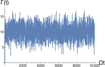
Figure 1: Decoherence rate function $\Gamma(t)$ for finite oscillator bath with only 10 fundamental frequencies with irrational ratios. $\Gamma(t)$ starts at zero and increases to average value of about $10$. It fluctuates most of the times between $5-15$ and rarely reaches minimum values $2-3$, but it never returns to zero! Coherence is lost most of the times by at least by a factor of $e^{-5}$-$e^{-15}$. On the rare occasions when $\Gamma(t)$ becomes $\sim 2$ still $\sim 87\%$ of the coherence is lost, $e^{-2}\sim 1-87\%$.

This may be considered as rather a new type of irreversible processes which have not received enough attention in the literature. Here there is no heat exchange between the bath and the system because the interaction Hamiltonian is diagonal in the energy basis of the system. Furthermore, the bath is finite. Nevertheless, the system does not return to its initial state and the decoherence is true.

.2 Infinite Bath

For an infinite bath one may define a spectral density function as follows Blencowe2013 ,

$$J(\omega)=\pi\omega_{0}^{2}\sum_{i}\lambda_{i}^{2}\delta(\omega-\omega_{i})$$ (34)

Then $\Gamma(t)$ of Eq. (22) can be written in terms of the spectral density function for an arbitrary temperature as

$$\Gamma(t)=\frac{1}{\pi}\int J(\omega)\frac{1-\cos\omega t}{\omega^{2}}\coth(\omega/2k_{B}T)\ d\omega$$ (35)

The integration is over the bandwidth that the frequencies of the bath oscillator make. We assume that the infinite oscillators make a continuum of frequencies and a smooth spectral density function $J(\omega)$. Further we assume that the frequencies have lower $\omega_{L}$ and upper $\Lambda$ cutoffs. For the ohmic spectral density of Ref. Blencowe2013 we adapt a sharp lower cutoff and a smooth upper cutoff as follows

$$J(\omega)=C\ \omega\ e^{-\omega/\Lambda}\ \theta(\omega-\omega_{L})$$ (36)

where $C$ is system-bath dimensionless coupling constant and $\theta(x)$ is the Heaviside step function. Using the results of Schlosshauer2007 we take the integral (35) for $k_{B}T\ll\Lambda$. The result is

$$\Gamma(t)=\Gamma_{vac}(t)+\Gamma_{therm}(t)$$ (37)

where

$$\Gamma_{vac}(t)=\frac{C}{2\pi}\ln(1+\Lambda^{2}t^{2})$$ (38)

is the vacuum fluctuation decoherence rate function and

$$\Gamma_{therm}(t)\approx\frac{C}{\pi}\ln\left[\frac{\sinh(\pi k_{B}Tt)}{\pi k_{B}Tt}\right]-\frac{C}{\pi}k_{B}T\ \omega_{L}\ t^{2}$$ (39)

is the thermal fluctuation decoherence rate function due to the bath.

At $T=0$, the thermal fluctuation vanishes and the decoherence is entirely due to the vaccum

$$\Gamma(t)=\Gamma_{vac}(t)$$ (40)

This is the case that cannot be obtained by use of Born-Markov approximation Blencowe2014pc

For small and finite temperatures and short times, i.e. $k_{B}Tt\ll 1$, the thermal fluctuation term becomes

$$\Gamma_{therm}\approx\frac{1}{\pi}Ck_{B}T(\frac{\pi^{2}}{6}k_{B}T-\omega_{L})t^{2}$$ (41)

Finally for high temperatures and longer times where one has $\Lambda\gg k_{B}T\gg 1/t\gg\omega_{L}$ one recovers the Born-Markov approximation result to leading order,

$$\Gamma(t)\approx Ck_{B}Tt$$ (42)

which agrees with Ref. Blencowe2013 .

.3 Summary

In summary we found almost exactly the decoherence rate of the toy model of gravitationally induced decoherence problem without use of Born-Markov approximation. We found that the off diagonal matrix elements decay as

$$\rho_{S}^{nm}(t)=\rho_{S}^{nm}(0)e^{-(n-m)^{2}[\Gamma_{vac}(t)+\Gamma_{therm}(t)]}$$ (43)

In the high temperature limit we recovered the result of Born-Markov approximation while at zero temperature we found that the thermal decoherence vanishes and the dominant decoherence is governed by the vacuum fluctuation.

For the finite bath we found that decoherence takes place unless the ration of fundamental frequencies of the bath are rational numbers.

References

• [1] Markus Aspelmeyer, TobiasΒ J. Kippenberg, and Florian Marquardt. Cavity optomechanics. Rev. Mod. Phys., 86:1391–1452, Dec 2014.
• [2] Dionys Baeriswyl, AlanΒ R Bishop, and JΒ Camelo. Applications of statistical and field theory methods to condensed matter, volume 218. Plenum Press, 1989.
• [3] M.Β P. Blencowe. Effective field theory approach to gravitationally induced decoherence. Phys. Rev. Lett., 111:021302, Jul 2013.
• [4] M.P. Blencowe. personal communication.
• [5] A.O Caldeira and A.J Leggett. Quantum tunnelling in a dissipative system. Annals of Physics, 149(2):374 – 456, 1983.
• [6] SeyyedΒ MH Halataei. Generalization of Caldeira-Leggett heat bath model for arbitrary quantum environments. "To appear", 2017.
• [7] MaximilianΒ A Schlosshauer. Decoherence: and the quantum-to-classical transition. Springer Science & Business Media, 2007.