Orbits for the Impatient: A Bayesian Rejection Sampling Method for Quickly Fitting the Orbits of Long-Period Exoplanets

Abstract

We describe a Bayesian rejection sampling algorithm designed to efficiently compute posterior distributions of orbital elements for data covering short fractions of long-period exoplanet orbits. Our implementation of this method, Orbits for the Impatient (OFTI), converges up to several orders of magnitude faster than two implementations of MCMC in this regime. We illustrate the efficiency of our approach by showing that OFTI calculates accurate posteriors for all existing astrometry of the exoplanet 51 Eri b up to 100 times faster than a Metropolis-Hastings MCMC. We demonstrate the accuracy of OFTI by comparing our results for several orbiting systems with those of various MCMC implementations, finding the output posteriors to be identical within shot noise. We also describe how our algorithm was used to successfully predict the location of 51 Eri b six months in the future based on less than three months of astrometry. Finally, we apply OFTI to ten long-period exoplanets and brown dwarfs, all but one of which have been monitored over less than 3 % of their orbits, producing fits to their orbits from astrometric records in the literature.

I. Introduction

Direct imaging is sensitive to substellar objects with large projected separations from their host objects ($\gtrsim$0.2 ”; e.g. Macintosh:2014, Claudi:2016), corresponding to larger orbital semi-major axes and periods compared to those detected with radial velocity and transit methods (Bowler:2016). Therefore, over timescales of months to years, direct imaging observations often probe only short fractions of these orbits. In these cases, constraints on orbital parameters can be used to perform a preliminary characterization of the orbit (e.g. Beust:2014, Nielsen:2014, Millar-Blanchaer:2015, Sallum:2015, DeRosa:2015, Zurlo:2016, Rameau:2016). Orbital parameter constraints can also lead to mass constraints on directly imaged substellar objects (e.g. Lagrange:2012, Fabrycky:2010), constraints on additional planets in the system (Bryan:2016), and information about the interactions between planets and circumstellar disks (e.g. Nielsen:2014, Millar-Blanchaer:2015, Rameau:2016). In addition, orbit fitting can be used to constrain the future locations of exoplanets, notably to calculate the probability of a transit (e.g. Wang:2016), or to determine an optimal cadence of observations to reduce uncertainty in orbital parameter distributions. For future direct imaging space missions such as the Wide-Field Infrared Survey Telescope (WFIRST; Spergel:2015, Traub:2016), it is particularly important to quickly and accurately fit newly discovered exoplanet orbits in order to plan future observations efficiently.

Several orbital fitting methods are currently used in astronomy. The family of Bayesian Markov Chain Monte Carlo methods (MCMC) was introduced to the field of exoplanet orbit fitting by Ford (2004, 2006) and has been widely used (e.g. Nielsen:2014, Millar-Blanchaer:2015, Dupuy:2016). MCMC is designed to quickly locate and explore the most probable areas of parameter space for a particular set of data, and takes longer to converge as a parameter space becomes less constrained by data, as in the case of astrometry from a fraction of a long-period orbit. In addition, many types of MCMC algorithms can be inefficient at exploring parameter spaces if the corresponding $\chi^{2}$ surface is complicated (e.g. Ford:2004). Another commonly used tool for fitting orbits is the family of least-squares Monte Carlo (LSMC) methods (Press:1992), which uses a Levenberg-Marquardt minimization algorithm to locate the orbital fit with minimum $\chi^{2}$ value for a set of astrometry. Once the minimum $\chi^{2}$ orbit is discovered, this method then randomly varies the measured astrometry along Gaussian distributions defined by the observational errors. In cases where the parameter space is very unconstrained, this method often explores only the area closest to the minimum $\chi^{2}$ orbit, leading to biases against areas of parameter space with lower likelihoods. For example, Chauvin:2012 found significantly different families of solutions when using LSMC than when using MCMC for the same orbital data for $\beta$ Pic b. LSMC is therefore effective at finding the best-fit solution, but not well-suited to characterizing uncertainty by fully exploring the parameter space.

In this work, we present Orbits for the Impatient (OFTI), a Bayesian Monte Carlo rejection sampling method based on that described in Ghez:2008, and similar to the method described in Konopacky:2016. OFTI is designed to quickly and accurately compute posterior probability distributions from astrometry covering a fraction of a long-period orbit. We describe how OFTI works and demonstrate its accuracy by comparing OFTI to two independent MCMC orbit-fitting methods. We then discuss situations where OFTI is most optimally used, and apply OFTI to several sets of astrometric measurements from the literature.

II. The OFTI Algorithm

II.1. Method

OFTI, like other Bayesian methods, combines astrometric observations and uncertainties with prior probability density functions (PDFs) to produce posterior PDFs of orbital parameters. These orbital parameter posteriors allow us to better characterize systems, for example by predicting future motion or by directly comparing the orbital plane to the orbits of other objects in the system or the distribution of circumstellar material.

The basic OFTI algorithm consists of the following steps:

1. Monte Carlo Orbit Generation from Priors
2. Scale-and-Rotate
3. Rejection sampling

OFTI uses a modified Bayesian rejection sampling algorithm. Rejection sampling consists of generating random sets of parameters, calculating a probability for each value, and preferentially rejecting values with lower probabilities. For OFTI, the generated parameters are the orbital elements semi-major axis, $a$, period, $P$, eccentricity, $e$, inclination angle, $i$, position angle of nodes, $\Omega$, argument of periastron, $\omega$, and epoch of periastron passage, $T_{0}$. For Bayesian rejection sampling algorithms such as OFTI, the candidate density functions used to generate these random parameters are prior probability distributions.

II.1.1 Monte Carlo Orbit Generation from Priors

OFTI begins by generating an initial set of seven random orbital parameters drawn from prior probability distributions. In this work, we use a linearly descending eccentricity prior with a slope of -2.18 for exoplanets, derived from the observed distribution of exoplanets detected by the radial velocity method (Nielsen:2010). The use of this prior assumes that long-period exoplanets follow the same eccentricity distribution as the planets detected by the radial velocity method.While the shape of the eccentricity prior directly affects the shape of the eccentricity posterior, as we would expect, the posteriors of other parameters are less affected when changing between a linearly descending and a uniform prior (see section 3.1). We assume a purely random orientation of the orbital plane, which translates into a sin($i$) prior in inclination angle and uniform priors in the epoch of periastron passage and argument of periastron. That is, the inclination angle, position angle of nodes, and argument of periastron priors are purely geometric. OFTI initially generates orbits with $a$ = 1 au and $\Omega$ = $0\,^{\circ}$, but these values are altered in the following step. We note that OFTI can be easily run using different priors, making it useful for non-planetary systems and statistical tests.

II.1.2 Scale-and-Rotate

Once OFTI has generated an initial set of orbital parameters from the chosen priors, it performs a ”scale-and-rotate” step in order to restrict the wide parameter space of all possible orbits. This increases the number of orbits accepted in the rejection sampling step. The generated semi-major axis and position angle of nodes are scaled and rotated, respectively, so that the new modified set of parameters describes an orbit that intersects a single astrometric data point. OFTI also takes the observational uncertainty of the data point used for the scale-and-rotate step into account. For each generated orbit, random offsets are introduced in separation ($\rho$) and position angle ($\theta$) from Gaussian distributions with standard deviations equal to the astrometric errors at the scale-and-rotate epoch. These offsets are added to the measured astrometric values, and then the generated orbit is scaled-and-rotated to intersect the offset data point, rather than the measured data point. The scale-and-rotate step produces a uniform prior in $\Omega$, and imposes a $\log(a)$ prior in semi-major axis. The posterior distributions OFTI produces are independent of the epoch chosen for this step, but the efficiency of the method is not. Some choices of the scale-and-rotate epoch result in a much higher fraction of considered orbits being accepted, and so the orbit is fit significantly faster. In order to take advantage of this change in efficiency, our implementation of OFTI performs an initial round of tests that pick out the scale-and-rotate epoch resulting in the largest acceptance rate of orbits, then uses this epoch every subsequent time this step is performed. The scale-and-rotate step differentiates OFTI from a true rejection sampling algorithm.

II.1.3 Rejection Sampling

Using the modified semi-major axis and position angle of nodes values, OFTI generates predicted $\rho$ and $\theta$ values for all remaining epochs. OFTI then calculates the $\chi^{2}$ probability for the predicted astrometry given the measured astrometry and uncertainties. This probability, assuming uncorrelated Gaussian errors, is given by: p $\propto e^{-\chi^{2}/2}$.

Finally, OFTI performs the rejection sampling step; it compares the generated probability to a number randomly chosen from a uniform distribution over the range (0,1). If the generated probability is greater than this random number, the generated set of orbital parameters is accepted.

This process is repeated until a desired number of generated orbits has been accepted (see Figure 1). As with MCMC, histograms of the accepted orbital parameters correspond to posterior PDFs of the orbital elements.

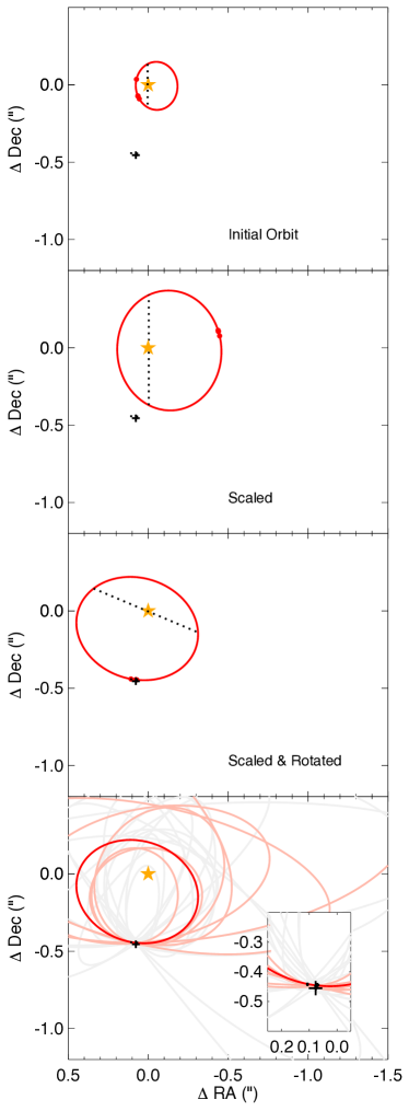
Figure 1.— Visualization of the OFTI method. Known astrometry (in this figure, for 51 Eri b), is shown as black crosses. The yellow star at (0,0) shows the location of 51 Eri A. Top: an orbit with $a$ = 1 au, $\Omega$ = $0\,^{\circ}$, and other orbital elements randomly drawn from appropriate priors is generated. Red dots along the orbit show the astrometric locations of 51 Eri b at the times of the observational epochs. The dotted line shows the line of nodes. Panels Two and Three: the scale-and-rotate step is performed. Bottom Panel: orbits accepted (light red) and rejected (gray) by the rejection sampling step of the OFTI algorithm. Inset: close up of bottom panel.

Our implementation of OFTI makes use of several computational and statistical techniques to speed up the basic algorithm described above:

• Our implementation uses vectorized array operations rather than iterative loops wherever possible. For example, instead of generating one set of random orbital parameters at a time, our program generates arrays containing 10,000 sets of parameters, and performs all subsequent operations on these arrays. Our program then iterates over this main loop, accepting and rejecting in batches of 10,000 generated orbits at a time. 10,000 is the empirically determined optimal number for our implementation.

• Our implementation of OFTI is written to run in parallel on multiple CPUs (our default is 10), speeding up runtime by a constant factor.

• Our implementation of OFTI is equipped with a statistical speedup that increases the fraction of orbits accepted per orbits tested. Due to measurement errors, the minimum $\chi^{2}$ orbit typically has a non-reduced $\chi^{2}$ value greater than 0. OFTI makes use of this fact by calculating the minimum $\chi^{2}$ value of all orbits tested during an initial run, then subtracting this minimum value from all future generated $\chi^{2}$ values, rendering them more likely to be accepted in the method’s rejection step. In rejection sampling, having a random variable whose range is greater than the maximum probability doesn’t change the distribution of parameters, but does result in more rejected trials.

• Our implementation of OFTI also restricts the ranges of the input $i$ and total mass priors based on initial results. After our implementation has accepted 100 orbits, it uses the maximum, minimum, and standard deviation of the array of accepted parameters to infer safe upper and lower limits to place on the relevant prior. This changes only the range of the relevant prior, not the shape of the prior. This speedup prevents our implementation of OFTI from wasting time generating orbits that have a negligible chance of being accepted.

II.2. Validation with MCMC

To illustrate that OFTI returns identical results to MCMC over short orbital arcs, we fit the same orbit and priors with OFTI and two MCMC orbit-fitting routines: the Metropolis Hastings MCMC algorithm described in Nielsen:2014, and an Affine Invariant MCMC Foreman-Mackey:2013 orbit fitter from (Macintosh:2014). In Figure 2, we plot the Metropolis Hastings MCMC and OFTI posterior PDFs calculated from astrometry of the system SDSS J105213.51+442255.7 AB (hereafter SDSS 1052; Dupuy:2015) from 2005-2006. SDSS 1052 is a pair of brown dwarfs with period of approximately 9 years. We chose only a subset of the available astrometry of SDSS 1052 to illustrate the effect of fitting a short orbital arc. In addition, we assume a fixed system mass, and we use astrometry provided in Table 2 of Dupuy:2015. The posterior distributions produced by OFTI and the Metropolis-Hastings MCMC are identical. OFTI was also validated using the relative astrometry of 51 Eri b, a directly imaged exoplanet discovered by the GPI Exoplanet Survey in 2015 (Macintosh:2015, DeRosa:2015). In Figure 3, we plot the posterior distributions produced by all three methods, calculated from relative astrometry of 51 Eri b taken between 2014 December and 2015 September. As in the previous case, all three sets of posterior distributions produced by OFTI and the two MCMC implementations are identical.

An important difference between MCMC and OFTI involves the types of errors on the posteriors produced by the two methods. Because each step of OFTI is independent of previous steps, deviations from analytical posteriors have the form of uncorrelated noise, i.e. if our implementation of OFTI is run until $100$ orbits are accepted, the output posteriors will not be biased, but simply noisy. As our implementation of OFTI is run until greater numbers of orbits are accepted, noise reduces by $\sqrt{N}$. MCMC steps, on the other hand, are not independent. Because the next MCMC step depends on the current location in parameter space, an un-converged MCMC run will result in biased, rather than noisy, posteriors. This is especially important in cases where MCMC has not been run long enough to achieve a satisfactory Gelman-Rubin (GR) statistic (a measure of convergence; Gelman:1992). In these cases, OFTI produces an unbiased result, while MCMC does not. This situation is illustrated in Figure 4, showing the posteriors produced by a Metropolis-Hastings implementation of MCMC and our implementation of OFTI for all known astrometry of ROXs 42B b (Currie:2014, Bryan:2016). After running for 30 hours on 10 CPUs, the MCMC posteriors are still un-converged, as can be seen by the lumpy shape of the $\Omega$ posterior. As a result, we see biases in the other posteriors. The GR statistics for each parameter were between 1.1 and 1.5 (an acceptable GR statistic is $\lesssim 1.01$, see e.g. Ford:2004). Our implementation of OFTI produced this result in 134 minutes, more than an order of magnitude faster than MCMC.

To demonstrate the differences in the random errors incurred by OFTI and the systematic errors of MCMC, and to illustrate OFTI’s computational speed for short orbital arcs, we calculated how the semi-major axis distributions generated by OFTI and MCMC changed as more sets of orbital elements were accepted for OFTI, and generated for MCMC. For both OFTI and MCMC, we calculate the median of the first $n$ semi-major axes tested as a function of $n$, resulting in an array of medians for OFTI and an array of medians for MCMC. We then take the ratio of each number in these arrays to the median of the complete distribution of tested semi-major axes. Since MCMC and OFTI converge on the same distributions, the medians of both complete semi-major axis distributions are the same. As $n$ approaches the total number of orbits tested, the partial distributions approach the complete distribution, and the ratios approach 1. We repeat this procedure for the lower and upper 1 $\sigma$ limits of the OFTI and MCMC semi-major axis distributions. These results are shown in Figure 5 for the orbit of 51 Eri b. Note that this represents the number of orbits tested, rather than number of orbits accepted, and so is directly proportional to computation time. After approximately $10^{4}$ orbits are tested, the OFTI semi-major axis distribution (red line) converges on the final median semi-major axis (to within 5 %), while the MCMC semi-major axis distribution (black line) suffers from systematic over- and under-estimates of the final semi-major axis value until more than 3 orders of magnitude more orbits have been tested. Similarly, OFTI converges on the appropriate 1 $\sigma$ upper and lower limits for the output semi-major axis distribution (to within 5 %) after approximately $10^{5}$ orbits are tested, while it takes MCMC $10^{8}$ correlated steps in order to do the same.

OFTI is most efficient for astrometry covering smaller fractions of orbits, while MCMC achieves convergence faster for larger fractions of orbits. Figure 6 illustrates this difference by displaying the wallclock time per CPU needed for each method to achieve convergence using astrometry from $\beta$ Pic b (Millar-Blanchaer:2015). In order to compare the time for convergence by MCMC and OFTI, we define a proxy for convergence time: our distributions are said to be “converged” for a statistic of interest (e.g. $a$ median, $i$ 68 % confidence interval) when the statistic is within 1$\,\%$ of the final value, where the final value is calculated from a distribution of $10^{4}$ accepted orbits.

For astrometry covering small fractions of a total orbit, OFTI can compute accurate future location predictions in much less time than MCMC. We illustrate this application in Figure 7, which shows probability distributions predicting the $\rho$, $\theta$ of 51 Eri b on 2015 September 15 from four earlier astrometric points taken over a timespan of less than 2 months (Macintosh:2015). Overplotted is the actual measured location of 51 Eri b. The predicted and observed medians for $\rho$ are $0.455\pm\,0.086$ and $0.4547\pm\,0.0057$, and for $\theta$ are $170\pm\,4$ and $166.5\pm\,0.6$. This prediction analysis was made before the most recent astrometric data were obtained. 51 Eri A was unobservable between February and September of 2015. It took OFTI less than 5 minutes (running in parallel on ten 2.3 GHz AMD Opteron 6378 processors) to produce these predictions.

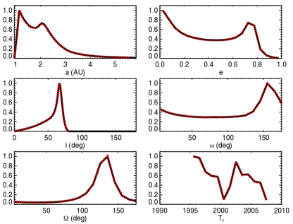
Figure 2.— Normalized PDFs of the orbital parameters corresponding to orbits accepted by OFTI (red) and MCMC (black) for astrometry of the  9 year period binary brown dwarf SDSS 1052 from 2005-2006. The PDFs are identical, differing only by shot noise.

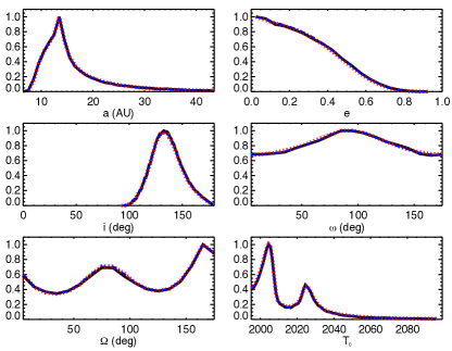
Figure 3.— Normalized PDFs of the orbital parameters corresponding to orbits accepted by OFTI (red), Metropolis-Hastings MCMC (black), and Affine-Invariant MCMC (blue) for relative astrometry of 51 Eri b from its discovery in 2014 December to 2015 September. The PDFs produced by all methods are identical, differing only by shot noise.

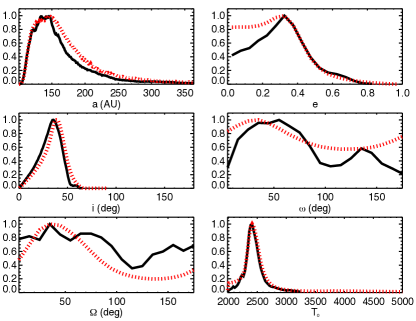
Figure 4.— Normalized PDFs of the orbital parameters produced by OFTI (red) and MCMC (black) for astrometry of ROXs 42B b. After approximately 30 hours of running in parallel on 10 cores, the MCMC chains are still unconverged, while OFTI produced $10^{6}$ permissible orbits in 134 minutes. The GR statistics for the MCMC chains plotted are all greater than 1.1, and the GR statistic for $\Omega$ is close to 1.5

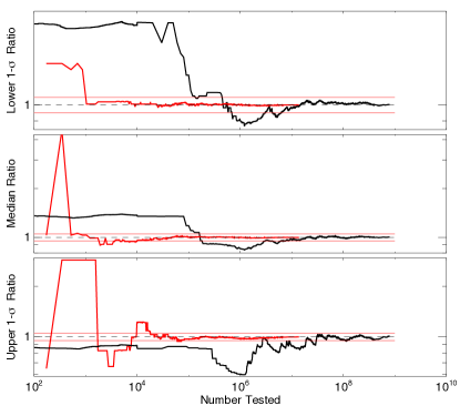
Figure 5.— Ratios of the partial and final lower 1 $\sigma$ limit, median, and upper 1 $\sigma$ limit for one Metropolis-Hastings MCMC chain (black), and one OFTI run (red), computed for all published astrometry of 51 Eri b. OFTI converges on the appropriate median solution after testing approximately $10^{4}$ sets of orbital elements, while MCMC continues to “wander” in a correlated fashion until accepting approximately $10^{7}$ orbits. Red horizontal lines are located at ratios of 1.05 and 0.95, and a black dashed line is located at a ratio of 1.00.

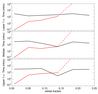
Figure 6.— Runtime per CPU needed for OFTI (red) and MCMC (black) to determine (within 1$\%\,$ error) the lower 1 $\sigma$ limit, median, and upper 1 $\sigma$ limit of the complete $a$ distribution, as a function of the orbital fraction covered by input astrometry of $\beta$ Pic b. As orbital fraction decreases, OFTI performance improves, while MCMC performance slightly improves. For orbital fractions greater than 15 %, we extrapolated the depicted behavior from the time OFTI took to accept 50 orbits.

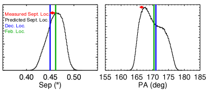
Figure 7.— PDFs in separation and position angle (black curves) predicting the location of 51 Eri b on 2015 September 15, given all previously known epochs of astrometry. The vertical blue lines show the astrometric location of 51 Eri b on 2015 February 1, the green lines the location on 2014 December 18, and the red horizontal bars the measured $\rho$, $\theta$.

II.3. Estimate of Performances

OFTI is a rejection-sampling method, meaning that it works by randomly sampling the parameter space of interest, then rejecting the sampled areas that do not match the data. As astrometry drawn from a larger fraction of the orbit becomes available, the orbit becomes more constrained, and the areas of parameter space that match the data shrink, so that OFTI becomes less efficient. A useful analogy for this phenomenon is throwing darts at a dartboard: when astrometry from only a small fraction of an orbit is available, many diverse orbits might fit the data, and a large fraction of the dartboard is acceptable, which results in a high acceptance rate. However, when more astrometry becomes available, a much smaller set of orbits will fit the data, and a much smaller fraction of the dartboard is acceptable, resulting in a lower acceptance rate.

Accordingly, OFTI is most efficient for astrometry covering a short fraction of an orbit, typically less than 15 % of the full orbital period. Because directly imaged exoplanets and brown dwarfs have large physical separations from their primary objects (greater than several au), OFTI is ideal for fitting the orbits of directly imaged systems, especially when the time spanned by direct imaging observations is short.

OFTI is also optimal when a quick estimate of the mean of a distribution is required. This will be particularly helpful in planning follow-up observations for space missions, as it allows to quickly estimate the optimal time for observations, also taking into account the possibility of the planet passing behind the star (see e.g. Savransky:2015). As Figure 5 shows, OFTI can converge on an estimate for the median of the 51 Eri b semi-major axis distribution within 5 % of the true median after fewer than $10^{4}$ orbits are tested. While an implementation of MCMC would have to run to completion in order to avoid a biased estimate of the semi-major axis distribution, the independence of successive OFTI trials allows OFTI to converge on an unbiased estimate much faster.

III. Applications

We use OFTI to fit orbits to 10 sets of astrometry from directly imaged exoplanets, brown dwarfs, and low-mass stars in the literature. Each substellar object has at least two published epochs of astrometry. We chose mostly objects for which an orbital fit has not been calculated because the available astrometry covers a short fraction of the object’s orbit. In performing these fits, we make the natural assumption that all objects are bound, and that all objects execute Keplerian orbits, as the chance of catching a common proper motion companion in the process of ejection or during the closest approach of two unassociated objects is particularly small.

We calculate fits using only the data available in the literature. Random and systematic errors in the astrometry available in the literature can bias these results. In particular, systematic errors in the measurement of plate scale or true north of the various instruments used to compile a single astrometric data set can significantly change orbit fits. Sharp apparent motion due to astrometric errors is likely to be fit as a higher eccentricity orbit; more astrometric data are needed to identify outliers of this nature.

For each substellar object, we compiled relative astrometry, distances, and individual object mass estimates from the literature (see Appendix). Values of the companion mass with error bars were given for 2M 1207 b, $\kappa$ And B, CD-35 2722 B, and GJ 504 b, and these were adopted as reported by the listed references. For HD 1160 B and C, $\eta$ Tel B, and HR 3549 B, no central value with error bars were given, but instead a range of masses was provided; in these cases we adopted the middle of the range. We note that for visual orbits mass of the system enters Kepler’s third law as the sum of the mass of both components, and so uncertainties in the orbit are dominated by uncertainties in the primary mass. We used Gaussian mass priors centered at the sum of the appropriate primary and secondary masses, with FWHM conservatively chosen to be the sum of the two mass uncertainties. For companion masses less than $15\,\%$ of the primary mass, which was the case for all objects except HIP 79797 B and 2M 1207, we neglected the uncertainty in the companion mass, and simply adopted the uncertainty of the primary. We used symmetric Gaussian priors in parallax or distance (we used distance priors only if no parallax was available in the literature), and symmetric or asymmetric Gaussian priors (asymmetric where asymmetric error bars were given) in total mass. Asymmetric Gaussian distributions consist of two half-Gaussians with individual $\sigma$ values, pieced together at the median of the aggregate distribution.

For each orbit, we provide:

• A table listing the maximum probability (maximum product of $\chi^{2}$ probability and prior probabilities), minimum $\chi^{2}$, median, 68 % confidence interval, and 95 % confidence interval orbital elements

• A triangle plot showing posterior distributions for each orbital element and 2-dimensional covariances for each pair of orbital elements

• A 3-panel plot showing 100 orbits drawn from the posterior distributions

III.1. GJ 504

GJ 504 b is the coldest and bluest directly-imaged exoplanet to date, and one of the lowest mass. Its discovery was reported by Kuzuhara:2013, who also perform a rejection-sampling orbit fit similar to OFTI (Janson:2011). Masses and astrometry are provided in Tables LABEL:tab:starparams and LABEL:tab:GJ504, and results are shown in Table LABEL:tab:gj504_outputs and Figures LABEL:fig:gj504_covariance and LABEL:fig:gj504_orbit. Our results are consistent with the posterior distributions they find (noting that Kuzuhara:2013 have used a flat prior in eccentricity). Using a linearly descending prior in eccentricity, we find a median semi-major axis of 48 au, with 68 % confidence between 39 and 69 au, and a corresponding period of 299 years, with 68 % confidence between 218 and 523 years. We also note that Kuzuhara:2013 find an $e$ posterior that decreases with eccentricity, as we do for OFTI calculations performed assuming both a uniform eccentricity prior and a linearly descending eccentricity prior.

We calculated fraction of orbital coverage by dividing the time spanned by observations by the 68 % confidence limits of the posterior distribution in period produced by OFTI. The calculated orbital fraction for the orbit of GJ 504 b is $0.4\,^{+0.1}_{-0.2}$ %.

To illustrate the impact of our choice of eccentricity prior on the results, we performed another fit to the astrometry of GJ 504 b using a uniform, rather than a linearly descending, prior in eccentricity. The results are shown in Figure LABEL:fig:prior_effect. The use of a different eccentricity prior changes the eccentricity posterior PDF, but does not significantly affect the other posterior PDFs. For example, when a linearly descending eccentricity prior is used, the semi-major axis posterior is $48\,^{+22}_{-9}$ au, and when a uniform eccentricity prior is used, the posterior shifts to $47\,^{+26}_{-11}$ au.

Table 1Orbit of GJ 504 b with respect to GJ 504 A

orbital element	unit	max probability	min $\chi^{2}$	median	68% confidence range	95% confidence range
$a$	au	44.48	67.24	48	39-69	31-129
$P$	yr	268.56	508.23	299	218-523	155-1332
$e$		0.0151	0.1519	0.19	0.05-0.40	0.01-0.62
$i$	∘	142.2	131.7	140	125-157	111-171
$\omega$	∘	91.7	4.9	95	31-151	4-176
$\Omega$	∘	133.7	61.6	97	46-146	8-173
$T_{0}$	yr	2228.11	2419.96	2145.10	2068.06-2310.13	2005.07-2825.03