Light spanners for bounded treewidth graphs imply light spanners for $H$-minor-free graphs

Abstract.

Grigni and Hung [10] conjectured that H-minor-free graphs have $(1+\epsilon)$-spanners that are light, that is, of weight $g(|H|,\epsilon)$ times the weight of the minimum spanning tree for some function $g$. This conjecture implies the efficient polynomial-time approximation scheme (PTAS) of the traveling salesperson problem in $H$-minor free graphs; that is, a PTAS whose running time is of the form $2^{f(\epsilon)}n^{O(1)}$ for some function $f$. The state of the art PTAS for TSP in H-minor-free-graphs has running time $n^{1/\mathrm{poly}(\epsilon)}$. We take a further step toward proving this conjecture by showing that if the bounded treewidth graphs have light greedy spanners, then the conjecture is true. We also prove that the greedy spanner of a bounded pathwidth graph is light and discuss the possibility of extending our proof to bounded treewidth graphs.

1. Introduction

Spanners are used to approximately preserve distances in a compact way. In this work, we focus on spanners that preserve distances within a $(1+\epsilon)$ factor (for a fixed $\epsilon<1$) and measure quality in terms of the spanner’s weight compared to the minimum spanning tree (the lightness). Formally, given an edge-weighted graph $G$, we wish to find a spanning subgraph $S$ of $G$ such that $d_{S}(x,y)\leq(1+\epsilon)\cdot d_{G}(x,y)\ \forall x,y\in V(G)$ and $w(S)=L(\epsilon)\cdot w(\mathrm{MST}(G))$ where the lightness, $L(\epsilon)$, is a function that depends only on $\epsilon$.

We focus on the greedy $(1+\epsilon)$-spanner, the spanner that is constructed by adding edges by increasing weight while doing so decreases the distance between their endpoints by a $1+\epsilon$ factor. Althöfer et al. showed that the greedy spanner has lightness $L(\epsilon)=O(1/\epsilon)$ for planar graphs (and also gave lightness bounds that depend on $n$ for general graphs) [1]. The same lightness bound holds for bounded genus graphs, as showed by Grigni [8]. However, the best lightness bound, which was shown by Grigni and Sissokho [11], for $H$-minor-free graphs is $(|H|\sqrt{\log|H|}\log n/\epsilon)$.

In this work, we investigate the possibility of removing the dependence on $n$ from the lightness for $H$-minor-free graphs by focusing on the following conjecture of Grigni and Hung [10]:

Conjecture .

$H$-minor-free graphs have $(1+\epsilon)$-spanners with lightness that depends on $|H|$ and $\epsilon$ only.

If this conjecture is true, it would, among other things, imply that TSP admits an efficient PTAS for $H$-minor free graph, that is, a PTAS whose running time is of the form $2^{f(\epsilon)}n^{O(1)}$ for some function $f$, improving on the existing PTAS with running time $n^{1/\mathrm{poly}(\epsilon)}$ via the framework of Demaine, Hajiaghayi and Kawarabayashi [3] and the spanner of Grigni and Sissokho [11]. We make progress towards proving Conjecture 1 by reducing the heart of the problem to the simpler graph class of bounded treewidth graphs:

Theorem 1.1.

If the greedy $(1+\epsilon)$-spanner of a graph of treewidth $\mathrm{tw}$ has lightness that depends on $\mathrm{tw}$ and $\epsilon$ only, then the greedy $(1+\epsilon)$-spanner of an $H$-minor-free graph has lightness that depends on $|H|$ and $\epsilon$ only.

Grigni and Hung gave a construction of a $(1+\epsilon)$-spanner for graphs of pathwidth $\mathrm{pw}$ with lightness $O(\mathrm{pw}^{3}/\epsilon)$ [10]; however, their construction is not greedy. Rather than considering the edges by increasing order of weight, they constructed a monotone spanning tree and greedily added edges to the monotone tree. They also argued that such a spanning tree is unlikely to exist for bounded treewidth graphs, giving little hope on two fronts (the different spanner construction as well as a construction that is unlikely to generalize to graphs of bounded treewidth) that Theorem 1.1 will lead to proving Conjecture 1 via Grigni and Hung’s work. In this paper we improve Grigni and Hung’s for bounded pathwidth graphs and do so by arguing lightness for the standard greedy algorithm, removing the limitations of Theorem 1.1 as a stepping stone to Conjecture 1. In Section 4, we prove:

Theorem 1.2.

The greedy $(1+\epsilon)$-spanner for a graph $G$ of pathwidth $\mathrm{pw}$ has lightness $O(\mathrm{pw}^{2}/\epsilon)$.

While our proof does not immediately extend to graphs of bounded treewidth, the techniques are not as specific to path decompositions as Grigni and Hung’s monotone-spanning-tree technique is, and thus gives more hope for proving Conjecture 1.

While it may seem like a limitation in proving Conjecture 1 that we must show that a particular construction of the $(1+\epsilon)$-spanner (namely the greedy construction) is light for bounded treewidth graphs, Filtser and Solomon (Theorem 4 [7]) showed that if an edge-weighted graph has light spanner, its greedy spanner is also light.

2. Analyzing greedy spanners

The greedy construction for a $(1+\epsilon)$-spanner due to Althöfer et al. [1] is an extension of Kruskal’s minimum spanning tree algorithm. Start by sorting the edges by increasing weight and an empty spanner subgraph $S$; for each edge $uv$ in order, if $(1+\epsilon)w(uv)\leq d_{S}(u,v)$, then $uv$ is added to $S$. By observing that this is a relaxation of Kruskal’s algorithm, $\mathrm{MST}(G)\subseteq S$. Althöfer et al. (Lemma 3 [1]) also showed that for any edge $e=uv$ in $S$ and any $u$-to-$v$ path $P_{S}(uv)$ between $u$ and $v$ in $S\setminus\{e\}$, we have:

$$(1+\epsilon)w(e)\leq w(P_{S}(uv))$$ (1)

The following property of greedy $(1+\epsilon)$-spanners is crucial in our analysis. The proof follows by contradiction to Equation (1) and can be found in Appendix B.

Lemma 2.1.

Let $S$ be the greedy $(1+\epsilon)$-spanner of a graph and let $H$ be a subgraph of $S$. Then the greedy $(1+\epsilon)$-spanner of $H$ is itself.

2.1. Charging scheme

To argue that $S$ is light, that is, has weight $L(\epsilon)w(\mathrm{MST}(G)$ for some function $L(\epsilon)$, we identify a specific charging path $P_{S}(uv)$ from $u$ to $v$ for each non-spanning-tree edge $uv$ of the spanner. One may think of $P_{S}(uv)$ as being the shortest $u$-to-$v$ path in $S$ when $uv$ is added to the spanner, but this is not necessary for the analysis; we only need that $(1+\epsilon)w(uv)\leq w(P_{S}(uv))$ (as is guaranteed by Equation (1) for greedy spanners) for every path in $S$. We call $(uv,P_{S}(uv))$ a charging pair. For a spanning tree $T$ (not necessarily a minimum spanning tree), we call a set of charging pairs $(e,P_{S}(e))$ for all edges $e\in S\backslash T$ a charging scheme. We say that an edge is charged to if it belongs to the charging path for another edge. A charging scheme is acyclic if for every edge $e\not\in T$, the directed graph where vertices of the graph are edges not in $T$ and directed edges represent charged to relationship, i.e. there is a directed edge $(e_{1}\rightarrow e_{0})$ if $e_{0}$ is charged to by $e_{i}$, is acyclic. A charging scheme is $k$-simple if each edge $e\in S\backslash T$ is charged to at most once and each edge in $T$ is charged to at most $k$ times. Based on these definitions , one can prove (see Appendix B for full details):

Lemma 2.2.

If $S$ is a greedy $(1+\epsilon)$-spanner of a graph that has a $k$-simple acyclic charging scheme to a spanning tree $T$, then $w(S)\leq(1+\frac{k}{\epsilon})w(T)$.

Indeed, in proving the greedy $(1+\epsilon)$-spanner has weight at most $(1+\frac{2}{\epsilon})\mathrm{MST}(G)$ when $G$ is planar, Althofer et al. [1] implicitly proved the existence of a 2-simple acyclic charging scheme to $\mathrm{MST}(G)$. Since our paper only deals with acyclic simple charging schemes, we simply say simple charging schemes to refer to acyclic simple charging schemes. We will use a stronger result for outer-planar graphs, planar graphs in which all the vertices are on the boundary of a common face (the outer face), which we take to be simple. The proof of the following lemma is included in Appendix B.

Lemma 2.3.

If $G$ is an outer-planar graph and $T$ is a path formed by all the edges in the boundary less one edge, then $G$ has an acyclic $1$-simple charging scheme to $T$.

For a greedy spanner $S$, one may instead, when it is convenient, define a weak $k$-simple charging scheme for a supergraph of $S$. A weak $k$-simple charging scheme is a $k$-simple charging scheme in which Equation (1) need not hold for charging pairs. See Appendix B for the proof of the following.

Lemma 2.4.

Let $S$ be a greedy spanner with spanning tree $T$ and let $\hat{S}$ be a supergraph of $S$ that $S$ spans. If $\hat{S}$ has a weak $k$-simple charging scheme to $T$ then $S$ has a $k$-simple charging scheme to $T$.

3. The greedy spanner of an $H$-minor free graph is possibly light

Our result relies on the Graph Minor Structure Theorem due to Robertson and Seymour [14] which guarantees a structural decomposition of an $H$-minor-free graph into simpler graphs. Informally, the seminal Graph Minor Structure Theorem of Robertson and Seymour states that every $H$-minor-free graph is the (small) clique-sum of graphs that are almost embeddable on graphs of small genus. We give a formal statement of the Graph Minor Structure Theorem below after some requisite definitions.

We first argue that almost-embeddable graphs have light $(1+\epsilon)$-spanners assuming bounded treewidth graphs have light $(1+\epsilon)$-spanners. We partition the spanner edges of almost-embeddable graphs into two parts: those in the surface-embeddable part and those in the non-embeddable part. We bound the weight of the surface-embeddable part by “cutting along” a subset of edges to create an outer-planar graph and then using the lightness bound for outer-planar graphs. Since the large-grid minor of the graph must be contained in the surface-embeddable part, we can show that the non-embeddable part has bounded treewidth. Therefore, the lightness of $(1+\epsilon)$-spanners of the non-embeddable part follows from the assumption that bounded treewidth graphs have light $(1+\epsilon)$-spanners.

3.1. Definitions: Treewidth, pathwidth and the structure of $H$-minor free graphs

Note that if $G$ excludes $K_{|H|}$ as a minor, then it also excludes $H$.

Tree decomposition

A tree decomposition of $G(V,E)$ is a pair $(\mathcal{X},\mathcal{T})$ where $\mathcal{X}=\{X_{i}|i\in I\}$, each $X_{i}$ is a subset of $V$ (called bags), $I$ is the set of indices, and $\mathcal{T}$ is a tree whose set of nodes is $\mathcal{X}$ satisfying the following conditions:

1. The union of all sets $X_{i}$ is $V$.

2. For each edge $uv\in E$, there is a bag $X_{i}$ containing both $u,v$.

3. For a vertex $v\in V$, all the bags containing $v$ make up a subtree of $\mathcal{T}$.

The width of a tree decomposition $\mathcal{T}$ is $\max_{i\in I}|X_{i}|-1$ and the treewidth of $G$, denoted by $\mathrm{tw}$, is the minimum width among all possible tree decompositions of $G$. A path decomposition of a graph $G(V,E)$ is a tree decomposition where the underlying tree is a path and is denoted by $(\mathcal{X},\mathcal{P})$. The pathwidth of a $G(V,E)$, denoted by $\mathrm{pw}$, is defined similarly.

$\beta$-almost-embeddable

A graph $G$ is $\beta$-almost-embeddable if there is a set of vertices $A\subseteq V(G)$ and $\beta+1$ graphs $G_{0},G_{1},\ldots,G_{\beta}$ such that:

1. $|A|\leq\beta$.

2. $G_{0}\cup G_{1}\cup\ldots\cup G_{\beta}=G[V\backslash A]$.

3. $G_{0}$ is embeddable in a surface $\Sigma$ of genus at most $\beta$.

4. Each $G_{j}$ has a path decomposition $(\mathcal{X}_{j},\mathcal{P}_{j})$ of width at most $\beta$ and length $|I_{j}|$, which is the number of bags, for $j\geq 1$.

5. There are $\beta$ faces $F_{1},F_{2},\ldots,F_{\beta}$ of $G_{0}$ such that $|F_{j}|\geq|I_{j}|$, $G_{0}\cap G_{j}\subseteq V(F_{j})$, and the vertices of $F_{j}$ appear in the bags of $\mathcal{X}_{j}$ in order along $\mathcal{P}_{j}$ for each $j$.

The vertices $A$ are called apices and the graphs $\{G_{1},G_{2},\ldots,G_{\beta}\}$ are called vortices. The vortex $G_{j}$ is said to be attached to the face $F_{j}$, $1\leq j\leq\beta$.

$\beta$-clique-sum

Given two graphs $H_{1},H_{2}$, a graph $H$ is called a $\beta$-clique-sum of $H_{1}$ and $H_{2}$ if it can be obtained by identifying a clique of size at most $\beta$ in each of two graphs $H_{1},H_{2}$ and deleting some of the clique edges.

We can now state Robertson and Seymour’s result:

Graph Minor Structure Theorem

(Theorem 1.3 [14]). An $H$-minor-free graph can be decomposed into a set of $\beta(|H|)$-almost-embeddable graphs that are glued together in a tree-like structure by taking $\beta(|H|)$-clique-sums where $\beta(|H|)$ is a function of $|H|$.

It will be convenient to consider a simplified decomposition that assumes there are no edges between the apices and vortices. This simplification introduces zero-weight edges that do not change the distance metric of the graph. We include the proof of this claim in Appendix B.

Claim 1.

There is a representation of a $\beta$-almost-embeddable graph as a $2\beta$-almost-embeddable graph that has no edge between apices and vertices of vortices (that are not in the surface-embedded part of the graph) and that maintains the distance metric of the graph.

In the remainder of this section, we prove Theorem 1.1 by assuming that, if $S$ is the greedy $(1+\epsilon)$-spanner of a graph of treewidth $\mathrm{tw}$:

$$w(S)\leq g(\mathrm{tw},\epsilon)\cdot w(\mathrm{MST})$$ (2)

The bulk of the technical detail in dealing with $H$-minor free graphs is in handling the vortices, which we do first.

3.2. Handling vortices

In this subsection, we consider a greedy $(1+\epsilon)$-spanner $G$ of some apex-free $\beta$-almost-embeddable graph. We will show that:

$$w(G)\leq q(\beta,\epsilon)\cdot w(\mathrm{MST}(G))$$ (3)

where $q(\beta,\epsilon)$ is the lightness that only depends on $\beta$ and $\epsilon$. Note that the MST of the graph is the MST of the spanner. We assume that $G$ is connected since we can bound the weight of each component separately. Let $G=G_{0}\cup G_{1}\cup\ldots\cup G_{\beta}$ be the decomposition of $G$ into a graph $G_{0}$ embedded on a surface $\Sigma$ of genus at most $\beta$ and a set $G_{1},\ldots,G_{\beta}$ vortices according to the definition of $\beta$-almost-embeddability. Let $C_{i}$ be the cycle bounding the face of $G_{0}$ to which vortex $G_{i}$ is attached.

Bounding the weight of the vortices First we bound the weight of the vortices and their bounding cycles $(\bigcup_{i=1}^{\beta}C_{i})\cup G_{i}$ by showing that $\mathrm{MST}(G)\cup(\bigcup_{i=1}^{\beta}C_{i}\cup G_{i})$ has bounded treewidth.

Let $K=(\mathrm{MST}(G)\cap G_{0})\cup\bigcup_{i=1}^{\beta}C_{i}$ and let $K^{*}$ be the dual of $K$; the vertices of $K^{*}$ correspond to the faces of $K$. Consider a vertex $v$ of $K^{*}$ that does not correspond to a face bounded by a cycle in $\{C_{1},C_{2},\ldots,C_{\beta}\}$. Then $v$ must be adjacent to a face that is bounded by a cycle $C_{j}$ for some $j$ because $K\setminus(\bigcup_{i=1}^{\beta}C_{i})$ is a forest. Therefore, the diameter of $K^{*}$ is $O(\beta)$. Since a graph of genus $\beta$ has treewidth $O(\beta\cdot\text{diameter})$ (Eppstein, Theorem 2 [5]), $K^{*}$ has treewidth $O(\beta^{2})$. Since the dual of a graph of treewidth $\mathrm{tw}$ and genus $\beta$ has treewidth $O(\mathrm{tw}+\beta)$ (Mazoit, Proposition 2 [13]), $K$ has treewidth $O(\beta^{2})$.

Grohe showed that if $G_{i}$ is a vortex attached to a face of $K$, then $\mathrm{tw}(G_{i}\cup K)\leq(\mathrm{pw}(G_{i})+1)(\mathrm{tw}(K)+1)-1$ (Lemma 2 [12]). Adding in each of the vortices $G_{1},G_{2},\ldots,G_{\beta}$ to $K$ and using Grohe’s result gives that the treewidth of $\mathrm{MST}(G)\cup(\bigcup_{i=1}^{\beta}C_{i}\cup G_{i})$ is $O(\beta^{\beta+2})$. Since $\mathrm{MST}(G)\cup(\bigcup_{i=1}^{\beta}C_{i}\cup G_{i})$ is the subgraph of a greedy spanner, $\mathrm{MST}(G)\cup(\bigcup_{i=1}^{\beta}C_{i}\cup G_{i})$ is a greedy spanner itself (Lemma 2.1) and by Equation (2), we have:

$$\textstyle\sum_{i=1}^{\beta}\left(w(C_{i})+w(G_{i})\right)\leq g(O(\beta^{\beta+2}),\epsilon)\cdot w(\mathrm{MST}(G)).$$ (4)

Bounding the surface-embedded part of the spanner Let $\widehat{G}$ be the graph obtained from $G_{0}$ by contracting the cycles $\{C_{1},C_{2},\ldots,C_{\beta}\}$ bounding the vortices into vertices $\{c_{1},c_{2},\ldots,c_{\beta}\}$, removing loops and removing parallel edges. Let $T_{\widehat{G}}$ be the minimum spanning tree of $\widehat{G}$ and let $X$ be the set of edges that has smallest summed weight such that cutting open the surface $\Sigma$ along $T_{\widehat{G}}\cup X$ creates a disk; $|X|\leq 2\beta$ (see, e.g. Eppstein [6]). Since $T_{\widehat{G}}\subseteq\mathrm{MST}(G)$ and an edge in the spanner is also the shortest path between its endpoints, we have:

$$w(T_{\widehat{G}}\cup X)\leq(2\beta+1)w(\mathrm{MST}(G))$$ (5)

Cutting the surface open along $X\cup T_{\widehat{G}}\cup\left(\bigcup_{i=1}^{\beta}C_{i}\right)$ creates $\beta+1$ disks: one disk for each face that a vortex is attached to and one disk $\Delta$ corresponding to the remainder of the surface. The boundary of $\Delta$, $\partial\Delta$, is formed by two copies of each of the edges of $T_{\widehat{G}}\cup X$ and one copy of each of the edges in $\cup_{i=1}^{\beta}C_{i}$ (see Figure 3 in Appendix C). Therefore we can use Equations (4) and (5) to bound the weight of the boundary of $\Delta$:

$$w(\partial\Delta)\leq(4\beta+2+g(O(\beta^{\beta+2}),\epsilon))\cdot w(\mathrm{MST}(G))$$ (6)

Let $E_{\Delta}$ be the set of edges of $G$ that are not in $\mathrm{MST}(G)$, $X$ or any of the vortices or their boundaries. That is, $E_{\Delta}$ contains all the edges that we have not yet bounded. Since $\partial\Delta$ spans $G_{0}$, there is a 1-simple charging scheme to $\partial\Delta$ (less an edge, Lemma 2.3). Therefore, by Lemma 2.2 and Lemma 2.1,

$$w(E_{\Delta})\leq(1+1/\epsilon)\cdot(4\beta+2+g(O(\beta^{\beta+2}),\epsilon))\cdot w(\mathrm{MST}(G))$$ (7)

Total weight of the spanner Since every edge of $G$ is either in $\mathrm{MST}(G)$, $X$, $E_{\Delta}$ or $G_{i}\cup C_{i}$ (for some $i$), summing Equations (4), (5) and (7) gives us Equation (3):

$$\begin{split}w(G)&\leq\underbrace{\left(2+2\beta+(1+1/\epsilon)(4\beta+2+g(O(\beta^{\beta+2}),\epsilon))+g(O(\beta^{\beta+2}),\epsilon)\right)}_{q(\beta,\epsilon)}w(\mathrm{MST}(G))\\ \end{split}$$ (8)

3.3. Adding apices and clique-sums

We are now ready to prove Theorem 1.1 by considering the apices and clique-sums of the decomposition. Let $G=J_{1}\oplus J_{2}\oplus\ldots\oplus J_{\gamma}$ be the $\beta(|H|)$-clique-sum of $\beta(|H|)$-almost-embeddable graphs $J_{1},J_{2},\ldots,J_{\gamma}$ given by the Graph Minor Structure Theorem. For $J_{i}$, let $A_{i}$ be its set of apices, let $J_{i}^{1},\ldots,J_{i}^{\beta}$ be its set of vortices and let $J_{i}^{0}$ be the graph embedded on a surface of genus at most $\beta$, as provided by the definition of $\beta(|H|)$-almost-embeddable. We assume the representation includes no edges between apices and the internal vertices of vortices (vertices that are not in $J_{i}^{0}$) by Claim 1.

Let $S$ be the greedy $(1+\epsilon)$-spanner of $G$. For each $J_{i}$, we define $S_{i}$ as the set of spanner edges in the apex-free $\beta(|H|)$-almost-embeddable part of $J_{i}$ (formally, $S_{i}=S\cap(\cup_{\ell}J_{i}^{\ell})$). Consider the spanning forest of $S_{i}$ that is induced by $\mathrm{MST}(G)$: $F_{i}=\mathrm{MST}(G)\cap S_{i}$. We choose a subset of edges $E_{i}$ of $S_{i}\backslash F_{i}$ such that:

1. The number of components of $F_{i}\cup E_{i}$ is minimized.

2. Subject to (i), the size of $E_{i}$ is minimized.

3. Subject to (i) and (ii), the weight of $E_{i}$ is minimized.

By the choice of $E_{i}$ and since $A_{i}$ has no edges to the internal vertices of vortices, each tree of $F_{i}\cup E_{i}$ is a minimum spanning tree for each apex-free $\beta(|H|)$-almost-embeddable component of $S_{i}$. Since $S_{i}$ is a subgraph of a greedy spanner, it is its own greedy spanner (Lemma 2.1) and so, by Equation (3), we have $w(S_{i})\leq q(\beta(|H|),\epsilon)(w(F_{i})+w(E_{i}))$. Summing over $i$, we have:

$$\begin{split}\textstyle\sum_{i=1}^{\gamma}w(S_{i})&\leq q(\beta(|H|),\epsilon)\textstyle\sum_{i=1}^{\gamma}\Big{(}w(F_{i})+w(E_{i})\Big{)}\\ &\leq q(\beta(|H|),\epsilon)\Big{(}w(\mathrm{MST}(G))+\textstyle\sum_{i=1}^{\gamma}w(E_{i})\Big{)}\end{split}$$ (9)

Let $S(A_{i})$ be edges of $S$ incident to vertices in $A_{i}$. Then, $S\cap J_{i}=S_{i}\cup S(A_{i})$ and hence $S=\bigcup_{i=1}^{\gamma}(S_{i}\cup S(A_{i}))$. Therefore, we have:

$$w(S)\leq\textstyle\sum_{i=1}^{\gamma}w(S_{i})+\textstyle\sum_{i=1}^{\gamma}w(S(A_{i}))$$ (10)

Now define $J_{i}^{\prime}=F_{i}\cup E_{i}\cup S(A_{i})$. Then $\mathrm{tw}(J_{i}^{\prime})\leq|A_{i}|+1\leq\beta(|H|)+1$. Let $G^{\prime}=J^{\prime}_{1}\oplus J^{\prime}_{2}\oplus\ldots\oplus J^{\prime}_{\gamma}$. We get that $\mathrm{tw}(G^{\prime})\leq\max_{i}\mathrm{tw}(J^{\prime}_{i})\leq\beta(|H|)+1$ by a result of Demaine et al. (Lemma 3 [4]). Note that $\mathrm{MST}(G^{\prime})=\mathrm{MST}(G)$. We have (by Lemma 2.1 and Equation (2)):

$$\textstyle\sum_{i=1}^{\gamma}w(F_{i})+w(E_{i})+w(S(A_{i}))\leq g(\beta(|H|)+1,\epsilon)\cdot w(\mathrm{MST}(G))$$ (11)

By Equations 9, 10 and 11, we get Theorem 1.1:

$$w(S)\leq\Big{(}(q(\beta(|H|),\epsilon)+1)\cdot g(\beta(|H|)+1,\epsilon)+q(\beta(|H|),\epsilon)\Big{)}w(\mathrm{MST}(G)).$$

4. The greedy spanner for bounded pathwidth graphs is light

Grigni and Hung proved that graphs of pathwidth $\mathrm{pw}$ have a $(1+\epsilon)$-spanner of lightness $O(\mathrm{pw}^{3}/\epsilon)$ [10]. They do so by building a spanning tree that is monotone with respect to the path decomposition of weight $O(\mathrm{pw}^{2})\,w(\mathrm{MST})$ (Lemma 2 [10]) and devising what we observe to be an $O(\mathrm{pw})$-simple charging scheme to the monotone spanning tree (Lemma 3 [10]). We prove that graphs of pathwidth $\mathrm{pw}$ have light greedy $(1+\epsilon)$-spanners by showing that there is an $O(\mathrm{pw}^{2})$-simple charging scheme to the $\mathrm{MST}$, forgoing the need for constructing a monotone spanning tree, giving Theorem 1.2. Our proof gives an evidence that one can avoid the pathwidth-specific monotonicity argument, opening a door to show that graphs of bounded treewidth may have light greedy $(1+\epsilon)$-spanners as well. We discuss the challenges for bounded treewidth graphs at the end of the paper. Throughout this section $G$ refers to the greedy $(1+\epsilon)$-spanner of some graph of pathwidth $\mathrm{pw}$.

Smooth decompositions

It will be convenient for our proofs to work with a standardized path decomposition. We assume that bags are ordered linearly, i.e, $X_{i}$ and $X_{i+1}$ are adjacent ($1\leq i\leq|I|-1$), and the path decomposition is smooth. A path decomposition $(\mathcal{X},\mathcal{P})$ is smooth if $|X_{i}|=\mathrm{pw}+1\quad\forall i\in I$ and $|X_{i}\cap X_{i+1}|=\mathrm{pw}$ for all $1\leq i\leq|I|-1$. Bodlaender [2] showed that a path decomposition can be turned into a smooth path decomposition of the same width in linear time. We root the path decomposition $(\mathcal{X},\mathcal{P})$ at the bag $X_{|I|}$.

For adjacent bags $X_{i},X_{i+1}$, we call the vertex in $X_{i+1}\backslash X_{i}$ the introduced vertex of $X_{i+1}$ and the vertex in $X_{i}\backslash X_{i+1}$ the forgotten vertex of $X_{i}$. All vertices of $X_{1}$ are introduced vertices and all vertices of $X_{|I|}$ are forgotten vertices.

Overview: designing an $O(\mathrm{pw}^{2})$-simple charging scheme

In designing an $O(\mathrm{pw}^{2})$-simple charging scheme, one needs to guarantee (i) each non-tree edge is charged at most once and (ii) each tree edge is charged at most $O(\mathrm{pw}^{2})$ times. At high level, we use the charging scheme for edges in $X_{0}\cup\ldots\cup X_{i-1}$ to design a charging scheme for the edges introduced to $X_{i}$. Let $u$ be the introduce vertex of $X_{i}$. We need to define charging pairs for all non-tree edges between vertices of $u$ and $X_{i}\setminus\{u\}$.

The simpler case is when there is a tree edge $uv$ incident to $u$ in $X_{i}$. For a non-tree edge $wu$ incident to $u$ in $X_{i}$, we define a charging path for $wu$ using the edges $uv$ (a tree edge) and $vw$ (an edge that already has a defined charging path since $vw$ is in a descendant bag of $X_{i}$). (This will be formalized as the triangle rule.) However, to guarantee condition (i), we must prevent the use of $wu$ in charging paths in the future. We keep track of this by way of a charging forest whose vertices are the edges of $G$; in this case we add an edge to the charging forest connecting $uv$ and $wu$.

The harder case is when there is no tree edge incident to $u$ in $X_{i}$. In this case, we consider the $u$-to-$v$ spanning-tree path that contains only edges of ancestor bags of $X_{i}$. We use this path as a sit-in for the edge $uv$ of the previous case. To guarantee condition (ii), we must be careful to not use tree-edges in ancestor bags too many times. Since $u$ may have an ancestral spanning-tree path to multiple vertices of $X_{i}\setminus\{u\}$, we delay the choice of which paths to use in defining a charging pair for edges incident to $u$ by adding dashed edges to the charging forest corresponding to all possible constructions. Then, to achieve condition (ii), we carefully select which dashed edges to convert in defining the charging pairs for edges incident to $u$ in $X_{i}$.

Normalized graph

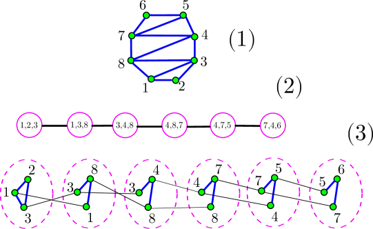
Figure 4. The normalized graph (3) of a graph (1) with path decomposition (2). Bold edges in (3) are edges of the original graph and thin edges in (3) are zero weighted edges.

We simplify the presentation of the formal argument, we use a normalized graph which merges a graph $G$ with its smooth path decomposition $(\mathcal{X},\mathcal{P})$. For each bag $X_{i}$, define the bag graph $G_{i}=(X_{i},E_{i})$ to be a subgraph of $G$ where $E_{i}$ is a maximal subset of edges of $G[X_{i}]$ incident to introduced vertices of $X_{i}$. This implies that each edge of $\mathrm{MST}(G)$ appears in exactly one bag graph. For adjacent bags $X_{i},X_{i+1}$, we add edges between two copies of the same vertex of $G$ in $G_{i}$ and $G_{i+1}$. We call the resulting graph the normalized graph of $G$ with respect to the path decomposition $(\mathcal{X},\mathcal{P})$ and denote it by $G_{\mathcal{P}}(V_{\mathcal{P}},E_{\mathcal{P}})$. We assign weight 0 to edges between bag graphs and weight $w(e)$ for the copy of the edge $e$ in $G$. See Figure 4 in Appendix C for an example. Since the distances between vertices in $G$ and the distances between their copies in $G_{\mathcal{P}}$ are the same: $w(\mathrm{MST}(G_{\mathcal{P}}))=w(\mathrm{MST}(G))$. Further, since distances are preserved, we can define a charging scheme for the greedy $(1+\epsilon)$-spanner of $G_{\mathcal{P}}$ to $\mathrm{MST}(G_{\mathcal{P}})$. In fact, we prove:

Theorem 4.1.

There is a $O(\mathrm{pw}^{2})$-simple charging scheme for the greedy $(1+\epsilon)$-spanner of $G_{\mathcal{P}}$ to $\mathrm{MST}(G_{\mathcal{P}})$.

This theorem, along with the equivalence of the metrics of $G_{\mathcal{P}}$ and $G$ and Lemma 2.2, gives Theorem 1.2. To simplify the construction of the charging scheme, we assume that $G$ is a $k$-path; this is without loss of generality by Lemma 2.4.

4.1. The charging forest

The main difficulty in defining the charging scheme is the existence of introduced vertices that are connected to the $\mathrm{MST}$ via an edge that is in an ancestor bag of the path decomposition. For the other types of introduced vertices, there is a triangle in the vertex’s bag graph that allows us to pay for the non-tree edges incident to that vertex. Throughout this section $\mathrm{MST}$ refers to $\mathrm{MST}(G_{\mathcal{P}})$.

To define the $O(\mathrm{pw}^{2})$-simple charging scheme, we construct a charging forest $\Phi$ to guide the charging. The charging forest is a rooted spanning forest of the line graph of $G$, with one tree rooted at a vertex corresponding to each edge of $\mathrm{MST}(G)$ (that is, each non-zero edge of the $\mathrm{MST}(G_{P})$). We call the nodes of $\Phi$ $\phi$-vertices and denote a $\phi$-vertex of $\Phi$ by $(u,v)$ where $uv$ is an edge of $G$.

We use three types of edges in constructing $\Phi$: dashed edges, bold edges and mixed edges. We construct $\Phi$ iteratively; $\Phi_{i}$ will be an intermediate forest of the line graph of $G[\cup_{j\leq i}X_{i}]$. $\Phi_{i}$ may contain all three types of edges but $\Phi=\Phi_{|I|}$ will contain only bold and mixed edges. From $\Phi_{i-1}$ to $\Phi_{i}$, a dashed edge may be deleted or converted to a mixed edge and newly added edges will either all be bold or all be dashed. A dashed-free tree of $\Phi_{i}$ is a maximal tree of $\Phi_{i}$ that contains no dashed edge. Trees of the intermediate forests may be unrooted, but each tree of an intermediate forest will contain at most one root.

We also maintain a contracted forest $\Lambda_{i}$ spanning vertices of $X_{i}$. Intuitively, $\Lambda_{i}$ tells us the connections between vertices of $X_{i}$ in $\mathrm{MST}[\cup_{j\leq i}X_{j}]$. $\Lambda_{i}$ is used to handle introduced vertices that have no tree edges to other vertices of the same bag. We also assign unique positive rank to each edge of $\mathrm{MST}$ in $G$ and assign rank 0 to all edges in $\mathrm{MST}$ added to $G_{\mathcal{P}}$ by the normalizing process. Ranks of edges of $\mathrm{MST}$ are used to define edge-rank in $\Lambda_{i}$ as follows: the rank of an edge $uv$ in $\Lambda_{i}$, denoted by $r_{i}(uv),$ is the minimum rank over the edges in the $u$-to-$v$ path of $\mathrm{MST}[\cup_{j\leq i}X_{i}]$. We assign rank to each edge of $\mathrm{MST}$ in a way that the rank of each edge in $\Lambda_{i}$ is unique.

The triangle rule

We say that an edge $((u,v),(u,w))$ of the line graph satisfies the triangle rule if $vw\in\mathrm{MST}(G)$ and $(u,v)$ and $(u,w)$ are in distinct dashed-free trees, both of which do not contain roots (i.e. $\phi$-vertices that correspond to edges of $\mathrm{MST}(G)$). We will add edges that satisfy the triangle rule to the charging forest. To maintain the acyclicity of the intermediate charging forests, if adding $((u,v),(u,w))$ introduces a cycle, the most recently added dashed edge on the path in the charging forest from $(u,v)$ to $(u,w)$ is deleted.

Invariants of the charging forest

Let $\Phi_{i}$ be the charging forest for $G_{\mathcal{P}}[\cup_{j\leq i}X_{j}]$. We say that a $\phi$-vertex $(u,v)$ of $\Phi_{i}$ is active if $u,v\in X_{i+1}$. We will show that $\Phi_{i}$ satisfies the following invariants:

1. For two trees $T_{1}$ and $T_{2}$ of $\mathrm{MST}[\cup_{j\leq i}X_{j}]$, all the $\phi$-vertices of the form $(u,v)$ such that $u\in T_{1}$ and $v\in T_{2}$ are in a common unrooted tree of $\Phi_{i}$. Further every unrooted tree of $\Phi_{i}$ contains $\phi$-vertices spanning components of $\mathrm{MST}[\cup_{j\leq i}X_{j}]$.

2. For a tree $T$ of $\mathrm{MST}[\cup_{j\leq i}X_{j}]$, all the $\phi$-vertices of the form $(u,v)$ such that $u,v\in T$ are in rooted dashed-free trees of $\Phi_{i}$.

3. Each unrooted dashed-free tree of $\Phi_{i}$ contains at least one active $\phi$-vertex.

4. For any $j\leq i$ and any two distinct trees $T_{1},T_{2}$ of $\mathrm{MST}[\cup_{\ell=j}^{i}X_{\ell}]$, $(y_{j,1},y_{j,2})$ and $(y_{i,1},y_{i,2})$ are in the same unrooted dashed-free tree of $\Phi_{i}$ where $y_{\ell,k}\in T_{k}\cap X_{\ell}$ for $\ell=i,j$ and $k=1,2$.

4.1.1. Initializing the charging forest

We define $\Phi_{1}$ as a forest of only bold edges. Recall that $G_{1}$ is a complete graph so there is a $\phi$-vertex for every unordered pair of vertices in $X_{1}$. We greedily include bold edges in $\Phi_{1}$ that satisfy the triangle rule. Equivalently, consider the subgraph $H$ of the line graph of $G_{1}$ consisting of edges $((u,v),(u,w))$ where $vw\in\mathrm{MST}$; $\Phi_{1}$ corresponds to any maximal forest of $H$ each tree of which contains at most one root ($\phi$-vertex corresponding to an edge of $\mathrm{MST}$).

We arbitrarily assign an unique rank to each edge of $\mathrm{MST}[X_{1}]$ from the set $\{1,2,\ldots,m_{1}\}$ where $m_{1}$ is the number of edges of $\mathrm{MST}[X_{1}]$ so that the highest-ranked edge is incident to the forgotten vertex of $X_{1}$. We define $\Lambda_{1}$ to be the forest obtained from $\mathrm{MST}[X_{1}]$ by contracting the highest-ranked edge incident to the forgotten vertex of $\mathrm{MST}[X_{1}]$. We observe that each edge in $\Lambda_{1}$ has a unique rank, since the rank of each edge of $\mathrm{MST}[X_{1}]$ is unique. We prove that $\Phi_{1}$ satisfies four invariants in Appendix B.

Claim 2.

Charging forest $\Phi_{1}$ satisfies all invariants.

4.1.2. Growing the charging forest

We build $\Phi_{i}$ from $\Phi_{i-1}$ and show that $\Phi_{i}$ will satisfy the invariants using the fact that $\Phi_{i-1}$ satisfies the invariants. Let $u$ be the introduced vertex of non-leaf bag $X_{i}$. If $u$ isolated in $\mathrm{MST}[X_{i}]$, we say that $u$ is a free vertex. The construction of $\Phi_{i}$ from $\Phi_{i-1}$ depends on whether or not $u$ is free.

$u$ is a free vertex

Let $\Lambda_{i-1}$ be the contracted forest of $X_{i-1}$. To obtain $\Phi_{i}$ from $\Phi_{i-1}$, we add $\phi$-vertices $(u,w)\quad\forall w\in(X_{i}\backslash\{u\})$ and add dashed edges $((u,w_{j}),(u,w_{k}))$ for each edge $w_{j}w_{k}$ in $\Lambda_{i-1}$. We assign rank to the dashed edge $((u,w_{j}),(u,w_{k}))$ to be the rank of $w_{j}w_{k}$ in $\Lambda_{i-1}$. We additionally change some dashed edges to mixed edges which we describe below. Since converting dashed edges to mixed edges does not affect these invariants, we have:

Claim 3.

Charging forest $\Phi_{i}$ satisfies Invariants (i), (ii) and  (iv).

We include the formal proof of Claim 3 in Appendix B.

Converting dashed edges to mixed edges

To ensure that $\Phi_{i}$ will satisfy Invariant (iii), we convert some dashed edges to mixed edges. First, consider the newly-added $\phi$-vertex $(u,v)$ where $v$ is the forgotten vertex of $X_{i}$. To ensure that $(u,v)$ will be in a dashed-free tree that contains an active $\phi$-vertex, we convert the added dashed edge $((u,v),(u,w))$, that has highest rank among newly added dashed edges, to a mixed edge. Second, suppose that $\tau$ is a dashed-free tree of $\Phi_{i-1}$ such that its active $\phi$-vertex is of the form $(v,w)$ for some $w\in X_{i}\backslash\{u\}$. The tree $\tau$ is at risk of becoming inactive in $\Phi_{i}$. However, by Invariant (i), $\tau$ is a subtree of a component $\hat{\tau}$ of $\Phi_{i-1}$ that consists of $\phi$-vertices $(u_{1},u_{2})$ such that $u_{k}\in T_{k}$ where $T_{k}$ is a component of $\mathrm{MST}[\cup_{j\leq i-1}X_{i}]$ for $k=1,2$. Further, since $T_{1}$ and $T_{2}$ must be connected in $\mathrm{MST}$ by a path through ancestor nodes of the path decomposition, there must be vertices in $T_{k}\cap X_{i+1}$; w.l.o.g., we take $(u_{1},u_{2})$ to be an active $\phi$-vertex in $\hat{\tau}$. We greedily convert dashed edges in $\hat{\tau}$ to mixed edges to grow $\tau$ until such an active $\phi$-vertex is connected to $(v,w)$ by mixed and bold edges, thus ensuring that $\Phi_{i}$ will satisfy Invariant (iii). We break ties between dashed edges for conversion to mixed edges by selecting the dashed edges that were first added to the charging forest and if there are multiple dashed edges which were added to the charging forest at the same time, we break ties by converting the dashed edges that have higher ranks to mixed edges. Note that by converting dashed edges into mixed edges, we add edges between dashed-free trees. Thus, Invariant (i), (ii), (iv) are unchanged.

Finally, we need to update $\Lambda_{i}$ from $\Lambda_{i-1}$. Let $\{v_{1},v_{2},\ldots,v_{q}\}$ be the set of neighbors of $v$ such that $r_{i-1}(vv_{1})\leq\ldots\leq r_{i-1}(vv_{q})$. Delete $v$ from $\Lambda_{i-1}$ and if $q\geq 2$, add edges $v_{j}v_{j+1}$ ($1\leq j\leq q-1$) to $\Lambda_{i-1}$ to obtained the forest $\Lambda_{i}$. Then, by definition, $r_{i}(v_{j}v_{j+1})=r_{i-1}(vv_{j})$ and $r_{i}(xy)=r_{i-1}(xy)$ for all other edges of $\Lambda_{i}$. Thus, by induction hypothesis, the rank of each edge of $\Lambda_{i}$ is unique.

$u$ is not a free vertex

To build $\Phi_{i}$ from $\Phi_{i-1}$, we add $\phi$-vertices $(u,w)\forall w\in X_{i}\backslash\{u\}$ and greedily add bold edges that satisfy the triangle rule. We include the formal proof that $\Phi_{i}$ satisfies Invariant (i), (ii), and  (iv) in Appendix B.

Claim 4.

Charging forest $\Phi_{i}$ satisfies Invariants (i), (ii) and  (iv).

We show that $\Phi_{i}$ satisfies Invariant (iii) here. Let $v$ be the forgotten vertex of $X_{i}$. Note that $u$ may have no tree edge to the forgotten vertex of $X_{i}$. In this case, we will ensure that previously active $\phi$-vertices of the form $(v,w)$ for $w\in X_{i}$ get connected to dashed-free trees that contain active $\phi$-vertices, we convert dashed edges to mixed edges. We do so in the same way as for the above described method for when $u$ was a free vertex, guaranteeing that $\Phi_{i}$ will satisfy Invariant (iii). Otherwise, we consider two subcases:

1. If $u=v$, then any $\phi$-vertex that was active in $\Phi_{i-1}$ is still active in $\Phi_{i}$. Thus, $(u,w)$ is connected to existing $\phi$-vertices that remain active for any $w\in X_{i}\setminus\{u\}$.

2. If $u\neq v$, then $\phi$-vertex $(x,v)$ will become inactive in $\Phi_{i}$. However, $(x,v)$ is connected to $(x,u)$ by the triangle rule or it was already connected to a root in a dashed-free tree. In either case, $\Phi_{i}$ satisfy Invariant (iii).

Finally, we show how to update $\Lambda_{i}$. Let $v$ be the forgotten vertex of $X_{i}$ and $u_{1},u_{2},\ldots,u_{p}$ be neighbors of $u$ in $\mathrm{MST}[X_{i}]$ such that $u_{1}=v$ if $uv\in\mathrm{MST}[X_{i}]$. Let $r^{\prime}$ be the maximum rank of over ranked edges of $\mathrm{MST}[\cup_{j\leq i-1}X_{j}]$. We assign rank $r_{i}(u,u_{j})=r^{\prime}+j$ for all $1\leq j\leq p$. We will update $\Lambda_{i}$ from $\Lambda_{i-1}$ depending on the relationship between $u$ and $v$:

1. If $u=v$, then we add edges $p-1$ edges $u_{j}u_{j+1}$, $1\leq j\leq p-1$, to $\Lambda_{i-1}$.

2. If $u\not=v$ and $uv\in\mathrm{MST}[X_{i}]$, we replace $v$ in $\Lambda_{i-1}$ by $u$ and add $p$ edges $uu_{j}$ to $\Lambda_{i-1}$.

3. Otherwise, we add $u$ and $p$ edges $uu_{j}$ to $\Lambda_{i-1}$. Let $\{v_{1},v_{2},\ldots,v_{q}\}$ be the set of neighbors of $v$ such that $r_{i-1}(vv_{1})\leq\ldots\leq r_{i-1}(vv_{q})$. We delete $v$ from $\Lambda_{i-1}$ and add $q-1$ edges $v_{j}v_{j+1}$.

Claim 5.

Each edge of the forest $\Lambda_{i}$ has a distinct rank.

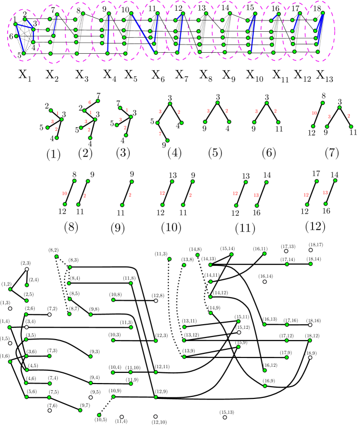
Figure 5. Top: A normalized graph and its MST. Dotted edges are non-tree edges. Non-dotted edges are edges of the MST. Thin edges are zero weighted edges. Center: Contracted forest $\Lambda_{1},\ldots,\Lambda_{12}$. Small numbers are ranks of the edges of the contracted forests. Bottom: Charging forest for the graph. Dotted edges are mixed edges. Hollow vertices are roots of the charging forest

We include the proof of Claim 5 in Appendix B. See Figure 5 in Appendix C for an example of a charging forest and contracted forests.

4.1.3. Using the charging forest to define an $O(\mathrm{pw}^{2})$-simple charging scheme

By Invariant (ii), all trees in $\Phi$ are rooted at $\phi$-vertices correspond to edges of $\mathrm{MST}$. Order the edges of $E(G)\backslash\mathrm{MST}(G)$ given by DFS pre-order of $\Phi$. Let $(u_{i-1},v_{i-1})$ and $(u_{i},v_{i})$ ($i\geq 2$) be two $\phi$-vertices of a component $T$ of $\Phi$ in this order. Define $P_{i}$ to be the (unique) $u_{i}$-to-$v_{i}$ path in $T\cup\{(u_{i-1},v_{i-1})\}$ that contains the edge $(u_{i-1},v_{i-1})$. We take $(P_{i},(u_{i},v_{i}))$ to be the charging pair for $(u_{i},v_{i})$. Note that the roots of $\Phi$ are edges of $\mathrm{MST}(G)$, so the charging paths are well-defined.

We prove that the charging scheme defined by the charging pairs is $O(\mathrm{pw}^{2})$-simple by bounding the number of times non-zero edges of $\mathrm{MST}$ are charged to. By the triangle rule, if $((u,v),(u,w))$ is a bold edge of $\Phi$, then $vw\in\mathrm{MST}$. We call the set of 3 vertices $\{u,v,w\}$ a charging triangle. If $((u,v),(u,w))$ is a mixed edge, $vw\notin\mathrm{MST}(G)$. In this case, we call $\{u,v,w\}$ a charging pseudo-triangle. The $v$-to-$w$ path in $\mathrm{MST}(G)$ is called the pseudo-edge; $vw$ is said to be associated with the charging (pseudo-) triangle. We say the edge $((u,v),(u,w))$ represents the charging (pseudo-) triangle.

Claim 6.

There are at most $\mathrm{pw}-2$ charging triangles associated with each non-zero edge of $\mathrm{MST}$.

Proof 4.2.

A charging triangle consists of one non-zero weight edge of $\mathrm{MST}$ and one edge not in the $\mathrm{MST}$ in the same bag graph. Note that each non-zero weight edge of $\mathrm{MST}$ is in exactly one bag graph and each bag graph has at most $\mathrm{pw}-2$ edges not in the $\mathrm{MST}$; that implies the claim.

The proof of the following is in Appendix B.

Lemma 4.3.

Each edge of $\mathrm{MST}(G)$ is in the paths corresponding to the pseudo-edges of at most $2\mathrm{pw}^{2}$ charging pseudo-triangles.

Consider each charging pair $(P_{i},(u_{i},v_{i}))$ in which $P_{i}$ contains $(u_{i-1},v_{i-1})$ that precedes $(u_{i},v_{i})$ in the DFS pre-order of a given component of $\Phi$. Let $(u_{i},v_{i})=(\hat{u}_{0},\hat{v}_{0}),\ldots,(\hat{u}_{t},\hat{v}_{t})=(u_{i-1},v_{i-1})$ be the set of $\phi$-vertices of the path between $(u_{i},v_{i})$ and $(u_{i-1},v_{i-1})$ in $\Phi$. We define $Q_{j}$ ($1\leq j\leq t$) be the $\hat{u}_{j-1}$-to-$\hat{v}_{j-1}$ path of $\mathrm{MST}\cup\{(\hat{u}_{j},\hat{v}_{j})\}$ containing edge $\hat{u}_{j}\hat{v}_{j}$. Then we have:

$$P_{i}=Q_{1}\ominus Q_{2}\ominus\ldots\ominus Q_{t}$$

where $\ominus$ is the symmetric difference between two sets. Hence, charging tree edges of $P_{i}$ is equivalent to charging the tree edges of $Q_{1},Q_{2},\ldots,Q_{t}$. We observe that tree edges of $Q_{j}$ are the tree edges of the (pseudo-) triangle represented by $((\hat{u}_{j},\hat{v}_{j}),(\hat{u}_{j-1},\hat{v}_{j-1}))$. Since each edge of $\Phi$ appears twice in the collection of paths between $(u_{i},v_{i})$ and $(u_{i-1},v_{i-1})$ in $\Phi$ for all $i$ and since different edges of $\Phi$ represents different charging (pseudo-) triangles, the tree edges of each charging (pseudo-) triangle are charged to twice. By Claim 6 and Lemma 4.3, each non-zero tree edge is charged to by at most $2(\mathrm{pw}-2)+2(2\mathrm{pw}^{2})=O(\mathrm{pw}^{2})$ times. Hence, the charging scheme is $O(\mathrm{pw}^{2})$-simple.

4.2. Toward light spanners for bounded treewidth graphs

The main difficulty in designing a simple charging scheme for bounded pathwidth graphs is the existence of free vertices. We introduce dashed edges to the charging forest when we handle free vertices and change a subset of dashed edges into mixed edges. By changing a dashed edge, say $((w,u),(w,v))$ into a mixed edge, we charge to the $u$-to-$v$ path in the MST once. Unfortunately, for bounded treewidth graphs, such charging can be very expensive. However, we observe that the $\phi$-vertex $(v,w)$ is contained in a rooted tree of $\Phi$. That means we can used $vw$ to charge to one of two edges $uv$ or $uw$. In general, for each non-tree edge $uv$ of the spanner in a bag $X_{i}$, we say $uv$ is a simple edge if $u,v$ are in the same component of the MST restricted to descendant bags of $X_{i}$ only or ancestor bags of $X_{i}$ only. Simple edges can be paid for in the spanner “cheaply”. Now, if $uv$ be an edge of the spanner in $X_{i}$ such that the $u$-to-$v$ path $P_{\mathrm{MST}}(u,v)$ of $\mathrm{MST}$ crosses back and forth through $X_{i}$. Let $w_{1},w_{2},\ldots,w_{k}$ be the set of vertices of $X_{i}$ in this order on the path $P_{\mathrm{MST}}(u,v)$. Then, we can charge the edge $uv$ by the set of simple edges $uw_{1},w_{1}w_{2},\ldots,w_{k}v$. We believe that this idea, with further refinement, will prove the existence of light spanners for bounded treewdith graphs.

Appendix A Notation

We denote $G=(V(G),E(G))$ to be the graph with vertex set $V(G)$ and edge set $E(G)$ and use $n,m$ to denote the number of vertices and edges, respectively. The order of $G$, denoted by $|G|$, is the number of vertices of $G$. Each edge $e$ of $E(G)$ is a assigned a weight $w(e)$. We define $w(H)=\sum_{e\in E(H)}w(e)$ to be the weight of edges of a subgraph $H$ of $G$. The minimum spanning tree of $G$ is denoted by $\mathrm{MST}(G)$. For two vertices $u,v$, we denote the shortest distance between them by $d_{G}(u,v)$. Given a subset of vertices $S$ and $u$ a vertex of $G$, we define $d_{G}(u,S)=\min_{v\in S}\{d_{G}(u,v)\}$ for $v=\arg\min_{v\in S}\{d_{G}(u,v)\}$. We omit the subscript $G$ when $G$ is clear from context. The subgraph of $G$ induced by $S$ is denoted by $G[S]$.

Appendix B Omitted Proofs

Proof B.1 (Proof of Lemma 2.1).

Let $S_{H}$ be the greedy $(1+\epsilon)$-spanner of $H$. We will prove that $S_{H}=H$. Note that $S_{H}$ is a subgraph of $H$ and shares the same set of vertices with $H$. Suppose for a contradiction that there is an edge $e=uv\in H\setminus S_{H}$. Since $uv$ is not added to the greedy spanner of $H$, there must be a $u$-to-$v$-path $P_{S_{H}}(uv)$ in $S_{H}$ that witnesses the fact that $uv$ is not added (i.e. $(1+\epsilon)w(e)>w(P_{S_{H}}(uv))$). However, $P_{S_{H}}(uv)\subseteq S$, contradicting Equation 1.

Proof B.2 (Proof of Lemma 2.2).

If $S$ has a $k$-simple charging scheme then:

$$(1+\epsilon)w(S\backslash T)\leq\sum_{e\in S\backslash T}w(P_{S}(e))\leq k\cdot w(T)+w(S\backslash T)$$

where the first inequality follows from edges in $S\backslash T$ having charging paths and the second inequality follows from each edge in $T$ appearing in charging paths at most $k$ times and each edge in $S\backslash T$ appearing in charging paths at most once. Rearranging the left- and right-most sides of this inequality gives us Lemma 2.2.

Proof B.3 (Proof of Lemma 2.3).

Let $e$ be the edge on the boundary of $G$ that is not in $T$. Let $T^{*}$ be the spanning tree of the dual graph containing all the edges that do not correspond to edges of $T$. We construct a charging scheme for $G$ by traversing $T^{*}$ in post-order, considering all the non-outer faces. Consider visiting face $f$ with children $f_{1},\ldots,f_{k}$ and parent $f_{0}$. Let $e_{i}$ be the edge of $G$ between $f$ and $f_{i}$ for all $i$ and let $P_{0}$ be the path between $e_{0}$’s endpoints in $T\cup\{e_{1},e_{2},\ldots,e_{k}\}$ that contains all the edges $\{e_{1},e_{2},\ldots,e_{k}\}$. Then, by Equation 1, $(e_{0},P_{0})$ is a charging pair for $e_{0}$. Also, since we visit $T^{*}$ in post-order, none of the edges $\{e_{1},e_{2},\ldots,e_{k}\}$ will be charged to when we build charging pairs for higher-ordered edges which are edges between faces of higher orders. Thus, the set of charging pairs produced from this process is a $1$-simple charging scheme to $T$.

Figure 1. An outer planar graph $G$. Bold edges are edges of $T$, dashed edges are non-tree edges and dotted edges are edges of the dual spanning tree, less the dual of $e$.

Proof B.4 (Proof of Lemma 2.4).

Consider an edge $\hat{e}\in\hat{S}\setminus S$. We first argue that $\hat{S}\setminus\{\hat{e}\}$ has a weak $k$-simple charging scheme. Since $T\subseteq S\cap\hat{S}$, $\hat{e}\notin T$ and so $\hat{e}$ can be charged to at most once. If $\hat{e}$ is in the charging path $P_{\hat{S}}(e)$ for another edge $e$ of $\hat{S}$, then we define the charging path for $e$ to be the simple path between $e$’s endpoints that is in $P_{\hat{S}}(e)\cup P_{\hat{S}}(\hat{e})\setminus\{\hat{e}\}$. The resulting set of paths is a weak $k$-simple charging scheme since every edge of $P_{\hat{S}}(\hat{e})$ is charged to one fewer time (by the removal of $\hat{e}$) and at most once more (by $e$).

By induction, $S$ has a weak $k$-simple charging scheme to $T$. Since $S$ is a greedy spanner, Equation (1) holds for every charging pair, so the weak $k$-simple charging scheme to $T$ is a $k$-simple charging scheme to $T$.

Proof B.5 (Proof of Claim 1).

Let $V_{a}$ be the set of vertices in vortex $V$ that are adjacent to apex $a$. Split vertex $a$ into two vertices $a$ and $a_{V}$ connected by a zero-weight edge so that $a_{V}$’s neighbors are $V_{a}\cup\{a\}$ and so that contracting the zero-weight edge gives the original graph. Add $a_{V}$ to all of the bags of the path decomposition of $V$. Now all the edges that connected $a$ to $V$ are within the vortex.

Consider the face in the surface-embedded part of the $\beta$-almost-embeddable graph to which $V$ is attached and let $xy$ be edge in that face that is between the first and last bags of $V$ and such that $y$ is in the first bag of $V$. Add the edges $xa_{V}$ and $a_{V}y$ to the embedded part of the graph and give them weight equal to the distance between their endpoints. Now $xa_{V}$ is the edge in that face that is between the first and last bags of the vortex and $a$ is adjacent to a vertex that is in the surface-embedded part of the $\beta$-almost-embeddable graph. See Figure 2.

The splitting of $a$ into $a_{V}$ increases the pathwidth of the vortex by 1. Repeating this process for all apex-vortex pairs increases the pathwidth of each vortex by at most $\beta$.

Figure 2. Apex $a$ and the vortices it is adjacent to before (a) and after (b) the reduction of Claim 1

Proof B.6 (Proof of Claim 2).

Note first that since there are only bold edges, the dashed-free trees of $\Phi_{1}$ are just the trees of $\Phi_{1}$.

Invarint (i)

Consider distinct trees $T_{1}$ and $T_{2}$ of $\mathrm{MST}[X_{1}]$ and consider $x,y\in T_{1}$ and $z\in T_{2}$. The $\phi$-vertices $(x,z)$ and $(y,z)$ are in the same component of $H$ as witnessed by the edges of the $x$-to-$y$ path in $T_{1}$. Further, $(x,z)$ cannot be connected to $(x,u)$ in $H$ where $xu\in\mathrm{MST}$ since that would imply $xz\in\mathrm{MST}$, contradicting that $T_{1}$ and $T_{2}$ are distinct trees of $\mathrm{MST}[X_{1}]$. Therefore, there is a maximal unrooted tree of $H$ that will contain all the $\phi$-vertices of the form $(u,v)$ such that $u\in T_{1}$ and $v\in T_{2}$.

Invariant (ii)

Consider a path $u_{0},u_{1},\ldots,u_{k}$ in $\mathrm{MST}[X_{1}]$ for $k\geq 2$; $((u_{0},u_{i}),(u_{0},u_{i+1}))$ are edges in $H$ for $i=1,\ldots,k-1$. Therefore $(u_{0},u_{1})$ (a root) and $(u_{0},u_{k})$ are in a common component of $H$. Therefore any maximal tree of $H$ that contains $(u_{0},u_{k})$ will contain a root.

Consider the component of $H$ described in showing $\Phi_{1}$ satisfies Invariant (i). Since $T_{1}$ and $T_{2}$ must be connected in $\mathrm{MST}$ by a path through ancestor nodes of the path decomposition, there is a vertex $u_{i}\in T_{i}$ such that $u_{i}\in X_{2}$ for $i=1,2$. Therefore $(u_{1},u_{2})$ is an active $\phi$-vertex in this component of $H$ and will be included in the maximal tree of this component.

Invariant (iv)

In this case, Invariant (iv) reduces to Invariant (i).

Proof B.7 (Proof of Claim 3).

We show that $\Phi_{i}$ satisfies Invariants (i), (ii) and  (iv) in turn:

1. The only new tree of $\mathrm{MST}[\cup_{j\leq i}X_{\ell}]$ compared to $\mathrm{MST}[\cup_{j\leq i-1}X_{\ell}]$ is $u$. For any pair of trees in $\mathrm{MST}[\cup_{\ell=j}^{i-1}X_{\ell}]$, Invariant (i) holds for $\Phi_{i}$ because it helps for $\Phi_{i-1}$. For a component $C$ of $\Lambda_{i-1}$, the addition of the edges $((u,w_{j}),(u,w_{k}))$ creates a new (unrooted) component spanning all $\phi$-vertices $(u,v)$ where $v$ is in the corresponding component of $\mathrm{MST}[\cup_{j\leq i}X_{j}]$. Therefore, Invariant (i) holds for $\Phi_{i}$.

2. Since $u$ is free and no new $\phi$-vertices of the form $(u,v)$ where $u$ and $v$ are in the same tree of $\mathrm{MST}[\cup_{j\leq i}X_{j}]$ are introduced, Invariant (ii) holds for $\Phi_{i}$ because it holds for $\Phi_{i-1}$.

3. As with $(i)$, the only new tree of $\mathrm{MST}[\cup_{\ell=j}^{i}X_{\ell}]$ is $u$, which only has a non-zero intersection with $X_{i}$. So, for $j<i$, Invariant (iv) holds for $\Phi_{i}$ because it holds for $\Phi_{i-1}$. For $j=i$, all the components of $\mathrm{MST}[\cup_{\ell=j}^{i}X_{\ell}]$ are isolated vertices, so the invariant holds trivially.

Proof B.8 (Proof of Claim 4).

We prove that $\Phi_{i}$ satisfies each of the invariants in turn.

Invariant (i)

Let $T_{1}$ and $T_{2}$ be distinct trees of $\mathrm{MST}[\cup_{j\leq i}X_{j}]$. If $T_{1}$ and $T_{2}$ are distinct trees of $\mathrm{MST}[\cup_{j\leq i-1}X_{j}]$, then the invariant holds for $\Phi_{i}$ because it holds for $\Phi_{i-1}$. Otherwise, we may assume w.l.o.g. that $T_{1}$ contains $u$ and a subtree $T_{3}$ that is a component of $\mathrm{MST}[\cup_{j\leq i-1}X_{j}]$. Let $x$ be a vertex of $T_{3}\cap X_{i}$ and $w$ be a vertex of $T_{2}\cap X_{i}$. Then $ux$ is an edge of $\mathrm{MST}$ and $(u,w),(w,x)$ will be connected in $\Phi_{i}$ by greedy applications of the triangle rule. By the same argument as used for showing that $\Phi_{1}$ satisfies Invariant (i), $(u,w)$ will not be connected to a root $\phi$-vertex (a $\phi$-vertex corresponding to a tree edge) in $\Phi_{i}$.

Invariant (ii)

We need only prove this for the tree $T$ of $\mathrm{MST}[\cup_{j\leq i}X_{i}]$ that contains $u$ as other cases are covered by the fact that $\Phi_{i-1}$ satisfies Invariant (ii). Let $T_{1}$ and $T_{2}$ be distinct trees of $\mathrm{MST}[\cup_{j\leq i-1}X_{i}]$ that are subtrees of $T$. Let $u_{1}$ and $u_{2}$ be vertices of $T_{1}\cap X_{i}$ and $T_{2}\cap X_{i}$, respectively.

We start by showing that $(u_{1},u_{2})$ is in a rooted dashed free tree of $\Phi_{i}$. Let $v_{1}$ and $v_{2}$ be the neighbors of $u$ in $T_{1}$ and $T_{2}$, respectively. (Note, it may be that, e.g., $u_{1}=v_{1}$.) By Invariant (ii), $(v_{2},u_{2})$ is in a rooted dashed-free tree of $\Phi_{i-1}$. By the triangle rule, $(v_{1},u_{2})$ will be connected by (a possibly non-trivial sequence of) bold edges to $(u,u_{2})$ which in turn will be connected by (a possibly non-trivial sequence of) bold edges to $(v_{2},u_{2})$. Therefore, $(v_{1},u_{2})$ will be in a rooted dashed-free tree of $\Phi_{i}$. In this next paragraph, we show that $(u_{1},u_{2})$ and $(v_{1},u_{2})$ are in the same dashed-free tree of $\Phi_{i-1}$, which we have just shown belongs to a rooted dashed-free tree of $\Phi_{i}$, showing that $(u_{1},u_{2})$ is in a rooted dashed free tree of $\Phi_{i}$.

To show that $(u_{1},u_{2})$ and $(v_{1},u_{2})$ are in the same dashed-free tree of $\Phi_{i-1}$, consider an index $k$ such that $u_{1}$ and $v_{1}$ are connected to $x_{1}$ in $\mathrm{MST}[\cup_{\ell=k}^{i}X_{\ell}]$ and $u_{2}$ is connected to $x_{2}$ in $\mathrm{MST}[\cup_{\ell=k}^{i}X_{\ell}]$. Then by Invariant (iv) for $\Phi_{i-1}$, $(x_{1},x_{2})$ is in the same dashed-free tree as $(u_{1},u_{2})$ and $(v_{1},u_{2})$.

Now consider a $\phi$-vertex $(x_{1},x_{2})$ where $x_{k}\in T_{k}\cap X_{j}$ for $k=1,2$ and $j<i$. Let $T_{k}^{\prime}$ be the subtree of $T_{k}$ that is in $\mathrm{MST}[\cup_{\ell=j}^{i-1}X_{\ell}]$ and let $u_{k}=T_{k}^{\prime}\cap X_{i}$ for $k=1,2$. We just showed that $(u_{1},u_{2})$ is in a rooted dashed-free tree of $\Phi_{i}$. By Invariant (iv) for $\Phi_{i-1}$, $(x_{1},x_{2})$ and $(u_{1},u_{2})$ are in the same dashed-free tree. Therefore, $(x_{1},x_{2})$ is in a rooted dashed-free tree of $\Phi_{i}$.

Invariant (iv)

Consider $j\leq i$, trees $T_{1},T_{2}$ of $\mathrm{MST}[\cup_{\ell=j}^{i}X_{\ell}]$, and $\phi$-vertices $(y_{j,1},y_{j,2})$ and $(y_{i,1},y_{i,2})$ as defined in Invariant (iv). For the case $j=i$, the proof that $\Phi_{i}$ satisfies Invariant (iv) is the same as for $\Phi_{1}$. Further, if $u\notin T_{1},T_{2}$, $\Phi_{i}$ satisfies Invariant (iv) because $\Phi_{i-1}$ satisfies Invariant (iv), therefore, we assume w.l.o.g. that $u\in T_{1}$. Finally, consider the components of $T_{1}$ in $\mathrm{MST}[\cup_{\ell=j}^{i-1}X_{\ell}]$; if $y_{j,1}$ and $y_{i,1}$ are in the same component, then $\Phi_{i}$ satisfies Invariant (iv) because $\Phi_{i-1}$ satisfies Invariant (iv). Therefore, we assume they are in different components, $T_{1}^{p}$ and $T_{1}^{q}$, respectively.

Let $x$ be the neighbor of $u$ in $T_{1}^{p}$. By Invariant (iv) for $\Phi_{i-1}$, $(x,y_{i,2})$ and $(y_{j,1},y_{j,2})$ are in a common unrooted dashed-free tree. We show that $(x,y_{i,2})$ and $(y_{i,1},y_{i,2})$ are in a common unrooted dashed-free tree of $\Phi_{i}$, proving this invariant is held. Let $y$ be the neighbor of $u$ in $T_{1}^{q}$.

1. By the triangle rule, $(x,y_{i,2})$ will get connected by (a possibly non-trivial sequence of) bold edges to $(u,y_{i,2})$ because $xu\in\mathrm{MST}$ and $(u,y_{i,2})$ will get connected by (a possibly non-trivial sequence of) bold edges to $(y,y_{i,2})$ because $yu\in\mathrm{MST}$.

2. Let $k$ be the index such that $y$ and $y_{i,1}$ are connected to $a$ in $\mathrm{MST}[\cup_{\ell=k}^{i}X_{\ell}]$ and $y_{i,2}$ is connected to $b$ in $\mathrm{MST}[\cup_{\ell=k}^{i}X_{\ell}]$. Then by Invariant (iv), $(a,b)$ is in the same unrooted dashed-free tree as $(y,y_{i,2})$ and $(y_{i,1},y_{i,2})$.

Together these connections show that $(x,y_{i,2})$ and $(y_{i,1},y_{i,2})$ are in a common unrooted dashed-free tree.

Proof B.9 (Proof of Claim 5).

We prove the claim for each case of the construction of $\Lambda_{i}$:

1. If $u=v$, we only add new edges to $\Lambda_{i-1}$ to obtain $\Lambda_{i}$. Since each added edge has distinct rank that is larger than the ranks of edges of $\Lambda_{i-1}$, the claim follows.

2. If $u\not=v$ and $uv\in\mathrm{MST}[X_{i}]$, since $r_{i}(xy)=r_{i-1}(xy)$ for any edge $xy$ such that $x,y\neq u$, we only need to consider the case when $u\in\{x,y\}$. Observe that for each neighbor $w$ of $u$, $r_{i}(uw)=r_{i-1}(vw)$ if $vw\in\Lambda_{i-1}$ or $uw$ is among the edges that are added to $\Lambda_{i-1}$. Since each newly added edge has unique rank, the claim follows.

3. Otherwise, we have $r_{i}(v_{j}v_{j+1})=r_{i-1}(v)v_{j}$ for $1\leq j\leq p-1$ and $r_{i}(xy)=r_{i-1}(xy)$ for all other edges. Thus, each edge in $\Lambda_{i}$ has unique rank by the induction hypothesis.

Let $w_{k}$ ($k=1,2$) be a vertex in $N^{r}_{i-1}(v_{k})\cup\{v_{k}\}$ such that:

Proof B.10 (Proof of Lemma 4.3).

We investigate how dashed edges are changed into mixed edges as this is when a charging pseudo-triangle arises. Recall that dashed edges are added to $\Phi$ when we process free vertices. Let $u$ be a free vertex that is introduced in bag $X_{i}$ and let $((u,v_{1}),(u,v_{2}))$ be a mixed edge (that is, a dashed edge in $\Phi_{i}$ that is later converted to a mixed edge). Then by our construction, $v_{1}$ and $v_{2}$ are in the same component of $\mathrm{MST}[\cup_{k\leq i-1}X_{k}]$. For each $j\geq i$ and $w\in X_{i}$, let $T^{ij}_{w}$ be the component of $\mathrm{MST}[\cup_{i\leq k\leq j}X_{k}]$ containing $w$. We will say that an introduced vertex of a bag $X_{j}$ is branching if it is not free, is not the forgotten vertex of $X_{j}$ and is not connected to the forgotten vertex of $X_{j}$ by $\mathrm{MST}$. Note that dashed edges are converted to mixed edges when processing free and branching vertices.

We say that a tree $T^{ij}_{w}\in\mathrm{MST}[\cup_{i\leq k\leq j}X_{k}]$ is forgotten in $X_{j}$ if $j=|I|$ or :

• $T_{w}^{ij}\cap X_{j}=\{v\}$ which is the forgotten vertex of $X_{j}$.

• the introduced vertex of $X_{j}$ is branching or free.

We note that at most one tree can be forgotten in each bag $X_{j}$.

For each vertex $x\in\Lambda_{i-1}$, let $N_{i-1}^{r}(x)$ be the set of vertices in $\Lambda_{i-1}$ reachable from $x$ via paths consisting of edges of ranks larger than $r$ in $\Lambda_{i-1}$. Let $F_{x,r}^{ij}=\cup_{w\in N_{i-1}^{r}(x)\cup\{x\}}T^{ij}_{w}$. We say that the forest $F_{x,r}^{ij}$ is forgotten in $X_{j}$ if every tree in $F_{x,r}^{ij}$ is forgotten in $X_{j^{\prime}}$ for some $j^{\prime}\leq j$ and $F_{x,r}^{ij}\cap X_{j}\not=\emptyset$.

Claim 7.

Let $r$ be the rank of the edge $v_{1}v_{2}\in\Lambda_{i-1}$. If the dashed edge $((u,v_{1}),(u,v_{2}))$ is changed into a mixed edge, there exists a bag $X_{j}$ for $j\geq i$ such that $T^{ij}_{u}\cap\{F^{ij}_{v_{1},r}\cup F^{ij}_{v_{2},r}\}=\emptyset$, $T^{ij}_{u}\cap X_{j}\not=\emptyset$ and exactly one of the forests $F_{v_{1},r}^{ij},F_{v_{2},r}^{ij}$ is forgotten in $X_{j}$.

Proof B.11.

Suppose that the claim fails, then there are two cases:

1. There exists $j\geq i$ such that $T^{ij}_{u}=T_{w}^{ij}$ for some $w\in F^{ij}_{v_{1},r}$ and $F^{ij}_{v_{2},r}\cap X_{j}\not=\emptyset$. In this case, $i<j$ since $u$ is a free vertex. Let $p$ be the index such that $u$ and $w$ are connected to $x$ in $\mathrm{MST}[\cup_{i\leq q\leq p}X_{q}]$. Let $w_{k}$ ($k=1,2$) be a vertex in $N^{r}_{i-1}(v_{k})\cup\{v_{k}\}$ such that:

   1. $T^{ij}_{w_{k}}\cap X_{p}\not=\emptyset$

   2. Subject to (i), the distance $d_{\Lambda_{i-1}}(w_{k},v_{k})$ is minimum.

   Let $y_{k}=T^{ij}_{w_{k}}\cap X_{p}$. Since the tie-breaking rule prefers changing the dashed edges of higher ranks into mixed edges, $(u,v_{k})$ is in the same dashed-free tree of $\Phi_{p}$ as $(u,w_{k})$. By Invariant (iv), $(u,w_{k})$ and $(w,w_{k})$ are in the same dashed-free tree of $\Phi_{p}$ as $(x,y_{k})$. Since $(w,w_{k})$ is in a rooted dashed-free tree of $\Phi_{p}$, by Invariant (i), $(u,v_{k})$ is in a rooted dashed free tree. Therefore, the dashed edge $((u,v_{1}),(u,v_{2}))$ is not converted to a mixed edge.

2. There exists $j\geq i$ such that $T^{ij}_{u}$ is forgotten and both forests $F^{ij}_{v_{1},r},F^{ij}_{v_{2},r}$ are not forgotten in $X_{j}$. Since $u$ is a free vertex, there must be a vertex $\hat{u}$ in $X_{i}$ such that $\hat{u}\in T^{ij}_{u}$. Let $p$ be the index such that $u$ and $\hat{u}$ are connected to $x$ in $\mathrm{MST}[\cup_{i\leq q\leq p}X_{q}]$. Let $w_{k}$ ($k=1,2$) be a vertex in $N_{i-1}^{r}(v_{k})\cup\{v_{k}\}$ as in the first case and $y_{k}=T^{ij}_{w_{k}}\cap X_{p}$. Then, by the tie-breaking rule, $(u,v_{k})$ and $(u,w_{k})$ are in the same dashed-free tree of $\Phi_{p}$. By Invariant (iv), $(u,w_{k})$ and $(\hat{u},w_{k})$ are in the same dashed-free tree of $\Phi_{p}$ as $(x,y_{k})$. Therefore, there is a cycle in which $((u,v_{1}),(u,v_{2}))$ is the most recent added dashed edge. Thus, $((u,v_{1}),(u,v_{2}))$ is deleted and not converted to a mixed edge.

We now bound the number of pseudo-triangles that contain an edge $e$ of $\mathrm{MST}(G)$. Let $X_{i}$ be the bag that containing $e$ and $\Lambda_{i}$ be the corresponding contracted forest. Let $u_{0},v_{0}$ be two vertices of $\Lambda_{i}$ in the same tree of $\Lambda_{i}$ such that $e$ is in the $u_{0}$-to-$v_{0}$ path $P_{\mathrm{MST}}(u_{0},v_{0})$. We say that a pseudo-triangle strongly contains $P_{\mathrm{MST}}(u_{0},v_{0})$ if $P_{\mathrm{MST}}(u_{0},v_{0})$ is a subpath of the pseudo-edge and the rank of every edge of the psedudo-edge of the triangle is at least the minimum rank over edges of $P_{\mathrm{MST}}(u_{0},v_{0})$.

Claim 8.

There are at most $\mathrm{pw}$ pseudo-triangles strongly containing $P_{\mathrm{MST}}(u_{0},v_{0})$.

Proof B.12.

Let $\Delta_{1},\ldots,\Delta_{q}$ be pseudo-triangles that strongly contain $P_{\mathrm{MST}}(u_{0},v_{0})$. Let $\Delta_{k}=\{u_{k},v_{k},w_{k}\}$ and $X_{s_{k}}$ be the bag that has $w_{k}$ as the introduced vertex ($1\leq k\leq q$). Let $r$ be the minimum rank over edges of $P_{\mathrm{MST}}(u_{0},v_{0})$ and $X_{\ell}$ be the bag in which one of the forests $F^{i\ell}_{u_{0},r},F^{i\ell}_{v_{0},r}$, say $F^{i\ell}_{u_{0},r}$, is forgotten. Then, $u_{k}\in F^{i\ell}_{u_{0},r}$ and $v_{k}\in F^{i\ell,r}_{v_{0}}$. We can assume w.l.o.g that $s_{1}\leq s_{2}\leq\ldots\leq s_{q}$. Then, $F_{u_{k},r}^{s_{k}\ell}=F^{i\ell}_{u_{0},r}\cap\mathrm{MST}[\cup_{s_{k}\leq j\leq\ell}X_{j}]$ and $F_{v_{k},r}^{s_{k}\ell}=F^{i\ell}_{v_{0},r}\cap\mathrm{MST}[\cup_{s_{k}\leq j\leq\ell}X_{j}]$. By Claim 7, $T^{s_{k}\ell}_{w_{k}}\cap X_{\ell}\not=\emptyset$. Furthermore, all the tree $T^{s_{k}\ell}_{w_{k}}$ must be disjoint since otherwise, say $T^{s_{j}\ell}_{w_{j}}$ is a subtree of $T^{s_{k}\ell}_{w_{k}}$ $(k\leq j)$, the second case of the proof of Claim 7 implies that the dashed edge $((w_{j},u_{j}),(w_{j},v_{j}))$ is removed from $\Phi$. Hence, $q\leq\mathrm{pw}$.

Let $e$ be an arbitrary edge of $\mathrm{MST}(G)$. Let $X_{i}$ be the bag that containing $e$ and $\Lambda_{i}$ be the corresponding contracted forest. By the way we build the contracted forest, there are at most two edges, say $u_{0}v_{0}$ and $v_{0}w_{0}$, of $\Lambda_{i}$ that are incident to the same vertex $v_{0}$ such that $e\in P_{\mathrm{MST}}(u_{0},v_{0})\cap P_{\mathrm{MST}}(v_{0},w_{0})$. We observe that any pseudo-triangle that contains $e$ in the pseudo-edge must contain the path $P_{\mathrm{MST}}(u,v)$ for some $u,v\in\Lambda_{i}$ such that one of two edges $u_{0}v_{0}$, $v_{0}w_{0}$ is in the path $P_{\Lambda_{i-1}}(u,v)$. Let $\Gamma(u_{0},v_{0})$ be the set of pseudo-triangles that have $P_{\Lambda_{i-1}}(u,v)$ containing $u_{0}v_{0}$. We define $\Gamma(v_{0},w_{0})$ similarly. We will show that $|\Gamma(u_{0},v_{0})|,|\Gamma(u_{0},w_{0})|\leq\mathrm{pw}^{2}$, thereby, proving the lemma.

We only need to show that $|\Gamma(u_{0},v_{0})|\leq\mathrm{pw}^{2}$ since $|\Gamma(u_{0},w_{0})|\leq\mathrm{pw}^{2}$ can be proved similarly. Let $\Delta_{1},\Delta_{2},\ldots,\Delta_{p}$ be the pseudo-triangles containing $e$ in the pseudo-forest such that for each $k$:

1. Each triangle $\Delta_{k}$ contains distinct path $P_{\mathrm{MST}}(u_{k},v_{k})$ as subpath in the pseudo-edge.

2. Edge $u_{0}v_{0}$ is in the path $P_{\Lambda_{i-1}}(u_{k},v_{k})$ of $\Lambda_{i-1}$.

3. Each path $P_{\mathrm{MST}}(u_{k},v_{k})$ has distinct rank.

Then, by the way we construct the contracted forest, if the minimum rank over edges of $P_{\mathrm{MST}}(u_{j},v_{j})$ is smaller than the minimum rank over edges of $P_{\mathrm{MST}}(u_{k},v_{k})$, then $P_{\Lambda_{i}}(u_{k},v_{k})\subsetneq P_{\Lambda_{i}}(u_{j},v_{j})$ for $1\leq j\not=k\leq p$. Therefore, we can rearrange $\Delta_{1},\Delta_{2},\ldots,\Delta_{k}$ such that $P_{\Lambda_{i}}(u_{1},v_{1})\subsetneq P_{\Lambda_{i}}(u_{2},v_{2})\subsetneq\ldots\subsetneq P_{\Lambda_{i}}(u_{p},v_{p})$. Thus, $p\leq\mathrm{pw}$ . By Claim 8, for each $k$, there are at most $\mathrm{pw}$ pseudo-triangles containing the same subpath $P_{\mathrm{MST}}(u_{k},v_{k})$. Therefore, $|\Gamma(u_{0},v_{0})|\leq\mathrm{pw}^{2}$.

Appendix C Figures

Figure 3. The surface $(2)$ is obtained by cutting the surface $\Sigma$ in $(1)$ along $T_{\widehat{G}}\cup X$. Small ovals are cycles $C_{1},C_{2},\ldots,C_{\beta}$.

References

- [1] I. Althofer, G. Das, D. Dobkin, D. Joseph, and L. Soares. On sparse spanners of weighted graphs. Discrete and Computational Geometry, 9(1):81–100, 1993.
- [2] H.L. Bodlaender. A linear time algorithm for finding tree-decompositions of small treewidth. In Proceedings of the 25th Annual ACM Symposium on Theory of Computing, STOC ’93, pages 226–234. ACM, 1993.
- [3] E. Demaine, M. Hajiaghayi, and K. Kawarabayashi. Contraction decomposition in -minor-free graphs and algorithmic applications. In Proceedings of the 43rd Annual ACM Symposium on Theory of Computing, page to appear, June 6–8 2011.
- [4] E. Demaine, M. Hajiaghayi, N. Nishimura, P. Ragde, and D. Thilikos. Approximation algorithms for classes of graphs excluding single-crossing graphs as minors. Journal of Computer and System Sciences, 69(2):166–195, 2004.
- [5] D. Eppstein. Diameter and treewidth in minor-closed graph families. Algorithmica, 27:275–291, 2000. Special issue on treewidth, graph minors, and algorithms.
- [6] D. Eppstein. Dynamic generators of topologically embedded graphs. In Proceedings of the 14th Annual ACM-SIAM Symposium on Discrete Algorithms, SODA ‘03, pages 599–608, 2003.
- [7] A. Filtser and S. Solomon. The greedy spanner is existentially optimal. In Proceedings of the 2016 ACM Symposium on Principles of Distributed Computing, PODC ’16, pages 9–17, 2016.
- [8] M. Grigni. Approximate tsp in graphs with forbidden minors. In Automata, Languages and Programming, volume 1853 of Lecture Notes in Computer Science, pages 869–877. Springer Berlin Heidelberg, 2000.
- [9] M. Sigurd and M. Zachariasen. Construction of Minimum-Weight Spanners. In Proceedings of the 12th Annual European Symposium on Algorithms, ESA’04, pages 797–808. Springer-Verlag, 2004.
- [10] M. Grigni and H. Hung. Light spanners in bounded pathwidth graphs. In Proceedings of the 37th International Conference on Mathematical Foundations of Computer Science, MFCS’12, pages 467–477. Springer-Verlag, 2012.
- [11] M. Grigni and P. Sissokho. Light spanners and approximate tsp in weighted graphs with forbidden minors. In Proceedings of the 13th Annual ACM-SIAM Symposium on Discrete Algorithms, SODA ’02, pages 852–857, Philadelphia, PA, US, 2002. Society for Industrial and Applied Mathematics.
- [12] M. Grohe. Local tree-width, excluded minors, and approximation algorithms. Combinatorica, 23(4):613–632, 2003.
- [13] F. Mazoit. Tree-width of hypergraphs and surface duality. Journal of Combinatorial Theory, Series B, 102(3):671–687, 2012.
- [14] N. Robertson and P.D. Seymour. Graph minors. XVI. Excluding a non-planar graph. Journal of Combinatorial Theory, Series B, 89(1):43–76, 2003.