Path-integral formalism for stochastic resetting:
Exactly solved examples and shortcuts to confinement

Abstract

We study the dynamics of overdamped Brownian particles diffusing in conservative force fields and undergoing stochastic resetting to a given location with a generic space-dependent rate of resetting. We present a systematic approach involving path integrals and elements of renewal theory that allows to derive analytical expressions for a variety of statistics of the dynamics such as (i) the propagator prior to first reset; (ii) the distribution of the first-reset time, and (iii) the spatial distribution of the particle at long times. We apply our approach to several representative and hitherto unexplored examples of resetting dynamics. A particularly interesting example for which we find analytical expressions for the statistics of resetting is that of a Brownian particle trapped in a harmonic potential with a rate of resetting that depends on the instantaneous energy of the particle. We find that using energy-dependent resetting processes is more effective in achieving spatial confinement of Brownian particles on a faster timescale than by performing quenches of parameters of the harmonic potential.

I Introduction

Changes are inevitable in nature, and those that are most dramatic with often drastic consequences are the ones that occur all of a sudden. A particular class of such changes comprises those in which the system during its temporal evolution makes a sudden jump (a “reset”) to a fixed state or configuration. Many nonequilibrium processes are encountered across disciplines, e.g., in physics, biology, and information processing, which involve sudden transitions between different states or configurations. The erasure of a bit of information Landauer:1961 ; Bennett:1973 by mesoscopic machines may be thought of as a physical process in which a memory device that is strongly affected by thermal fluctuations resets its state (0 or 1) to a prescribed erasure state Berut:2012 ; Mandal:2012 ; Roldan:2014 ; Koski:2014 ; Fuchs:2016 . In biology, resetting plays an important role inter alia in sensing of extracellular ligands by single cells Mora:2015 , and in transcription of genetic information by macromolecular enzymes called RNA polymerases Roldan:2016 . During RNA transcription, the recovery of RNA polymerases from inactive transcriptional pauses is a result of a kinetic competition between diffusion and resetting of the polymerase to an active state via RNA cleavage Roldan:2016 , as has been recently tested in high-resolution single-molecule experiments Lisica:2016 . Also, there are ample examples of biochemical processes that initiate (i.e., reset) at random so-called stopping times Gillespie:2014 ; Hanggi:1990 ; Neri:2017 , with the initiation at each instance occurring in different regions of space  Julicher:1997 . In addition, interactions play a key role in determining when and where a chemical reaction occurs Gillespie:2014 , a fact that affects the statistics of the resetting process. For instance, in the above mentioned example of recovery of RNA polymerase by the process of resetting, the interaction of the hybrid DNA-RNA may alter the time that a polymerase takes to recover from its inactive state Zamft:2012 . It is therefore quite pertinent and timely to study resetting of mesoscopic systems that evolve under the influence of external or conservative force fields.

Simple diffusion subject to resetting to a given location at random times has emerged in recent years as a convenient theoretical framework to discuss the phenomenon of stochastic resetting Evans:2011-1 ; Evans:2011-2 ; Evans:2014 ; Christou:2015 ; Eule:2016 ; Nagar:2016 . The framework has later been generalized to consider different choices of the resetting position Boyer:2014 ; Majumdar:2015-2 , resetting of continuous-time random walks Montero:2013 ; Mendez:2016 , Lévy Kusmierz:2014 and exponential constant-speed flights Campos:2015 , time-dependent resetting of a Brownian particle Pal:2016 , and in discussing memory effects Boyer:2017 and phase transitions in reset processes Harris:2017 . Stochastic resetting has also been invoked in the context of many-body dynamics, e.g., in reaction-diffusion models Durang:2014 , fluctuating interfaces Gupta:2014 ; Gupta:2016 , interacting Brownian motion Falcao:2017 , and in discussing optimal search times in a crowded environment Kusmierz:2015 ; Reuveni:2016 ; Bhat:2016 ; Pal:2017 . However, little is known about the statistics of stochastic resetting of Brownian particles that diffuse under the influence of force fields Pal:2015 , and that too in presence of a rate of resetting that varies in space.

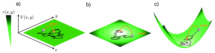
Figure 1: Stochastic resetting of Brownian particles moving in force fields and subject to stochastic resetting with a rate that may depend on space. Illustration of the motion of a single overdamped Brownian particle (grey sphere) that diffuses in two dimensions $(x,y)$ in presence of a conservative potential $V(x,y)$. The particle traces a stochastic trajectory (black curve) in the two-dimensional space until its position is reset at a random instant of time to its initial value (orange arrow); subsequent to the reset, the particle resumes its stochastic motion until the next reset happens. The rate of resetting $r(x,y)$ (left colorbar) may depend on the position of the particle. We study three different scenarios: a) Resetting of free Brownian particles under a space-independent rate of resetting; b) Resetting of free Brownian particles under a space-dependent rate of resetting; c) Resetting of Brownian particles moving in force fields under a space-dependent rate of resetting.

In this paper, we study the dynamics of overdamped Brownian particles immersed in a thermal environment, which diffuse under the influence of a force field, and whose position may be stochastically reset to a given spatial location with a rate of resetting that has an essential dependence on space. We use an approach that allows to obtain exact expressions for the transition probability prior to the first reset, the first reset-time distribution, and, most importantly, the stationary spatial distribution of the particle. The approach is based on a combination of the theory of renewals Cox:1962 and the Feynman-Kac path-integral formalism of treating stochastic processes Feynman:2010 ; Schulman:1981 ; Kac:1949 ; Kac:1951 , and consists in a mapping of the dynamics of the Brownian resetting problem to a suitable quantum mechanical evolution in imaginary time. We note that the Feynman-Kac formalism has been applied extensively in the past to discuss dynamical processes involving diffusion satya , and has to the best of our knowledge not been applied to discuss stochastic resetting. To demonstrate the utility of the approach, we consider several different stochastic resetting problems, see Fig. 1: i) Free Brownian particles subject to a space-independent rate of resetting (Fig. 1a)); ii) Free Brownian particles subject to resetting with a rate that depends quadratically on the distance to the origin (Fig. 1b)); and iii) Brownian particles trapped in a harmonic potential and undergoing reset events with a rate that depends on the energy of the particle (Fig. 1c)). In this paper, we consider for purposes of illustration the corresponding scenarios in one dimension, although our general approach may be extended to higher dimensions. Remarkably, we obtain exact analytical expressions in all cases, and, notably, in cases ii) and iii), where a standard treatment of analytic solution by using the Fokker-Planck approach may appear daunting, and whose relevance in physics may be explored in the context of, e.g., optically-trapped colloidal particles and hopping processes in glasses and gels. We further explore the dynamical properties of case iii), and compare the relaxation properties of dynamics corresponding to potential energy quenches and due to sudden activation of space-dependent stochastic resetting.

II General formalism

II.1 Model of study: resetting of Brownian particles diffusing in force fields

Consider an overdamped Brownian particle diffusing in one dimension $x$ in presence of a time-independent force field $F(x)=-\partial_{x}V(x)$, with $V(x)$ denoting a potential energy landscape. The dynamics of the particle is described by a Langevin equation of the form

$$\frac{{\rm d}x}{{\rm d}t}=\mu F(x)+\eta(t),$$ (1)

where $\mu$ is the mobility of the particle, defined as the velocity per unit force. In Eq. (1), $\eta(t)$ is a Gaussian white noise, with the properties

$$\langle\eta(t)\rangle=0,~{}\langle\eta(t)\eta(t^{\prime})\rangle=2D\delta(t-t^{\prime}),$$ (2)

where $\langle\,\cdot\,\rangle$ denotes average over noise realizations, and $D\!>\!0$ is the diffusion coefficient of the particle, with the dimension of length-squared over time. We assume that the Einstein relation holds: $D=k_{\rm B}T\mu$, with $T$ being the temperature of the environment, and with $k_{\rm B}$ being the Boltzmann constant. In addition to the dynamics (1), the particle is subject to a stochastic resetting dynamics with a space-dependent resetting rate $r(x)$, whereby, while at position $x$ at time $t$, the particle in the ensuing infinitesimal time interval ${\rm d}t$ either follows the dynamics (1) with probability $1-r(x){\rm d}t$, or resets to a given reset destination $x^{(\rm r)}$ with probability $r(x){\rm d}t$. Our analysis holds for any arbitrary reset function $r(x)$, with the only obvious constraint $r(x)\geq 0~{}\forall\,x$; moreover, the formalism may be generalized to higher dimensions. In the following, we consider the reset location to be the same as the initial location $x_{0}$ of the particle, that is, $x^{(\rm r)}=x_{0}$.

A quantity of obvious interest and relevance is the spatial distribution of the particle: What is the probability $P(x,t|x_{0},0)$ that the particle is at position $x$ at time $t$, given that its initial location is $x_{0}$? From the dynamics given in the preceding paragraph, it is straightforward to write the time evolution equation of $P(x,t|x_{0},0)$:

$$\frac{\partial P(x,t|x_{0},0)}{\partial t}=-\mu\frac{\partial(F(x)P(x,t|x_{0},0))}{\partial x}+D\frac{\partial^{2}P(x,t|x_{0},0)}{\partial x^{2}}$$

$$-r(x)P(x,t|x_{0},0)+\int{\rm d}y~{}r(y)P(y,t|x_{0},0)\delta(x-x_{0}),$$ (3)

where the first two terms on the right hand side account for the contribution from the diffusion of the particle in the force field $F(x)$, while the last two terms stand for the contribution owing to the resetting of the particle: the third term represents the loss in probability arising from the resetting of the particle to $x_{0}$, while the fourth term denotes the gain in probability at the location $x_{0}$ owing to resetting from all locations $x\neq x_{0}$. When exists, the stationary distribution $P_{\rm st}(x|x_{0})$ satisfies

$$0=-\mu\frac{\partial(F(x)P_{\rm st}(x|x_{0}))}{\partial x}+D\frac{\partial^{2}P_{\rm st}(x|x_{0})}{\partial x^{2}}$$

$$-r(x)P_{\rm st}(x|x_{0})+\int{\rm d}y~{}r(y)P_{\rm st}(y|x_{0})\delta(x-x_{0}).$$ (4)

It is evident that solving for either the time-dependent distribution $P(x,t|x_{0},0)$ or the stationary distribution $P_{\rm st}(x|x_{0})$ from Eqs. (3) and (4), respectively, is a formidable task even with $F=0$, unless the function $r(x)$ has simple forms. For example, in Ref. Evans:2011-2 , the authors considered a solvable example with $F(x)=0$, where the function $r(x)$ is zero in a window around $x_{0}$ and is constant outside the window.

In this work, we employ a different approach to solve for the stationary spatial distribution, by invoking the path integral formalism of quantum mechanics and by using elements of the theory of renewals. In this approach, we compute $P_{\rm st}(x|x_{0})$, the stationary distribution in presence of reset events, in terms of suitably-defined functions that take into account the occurrence of trajectories that evolve without undergoing any reset events in a given time, see Eq. (32) below. This approach provides a viable alternative to obtaining the stationary spatial distribution by solving the Fokker-Planck equation (4) that explicitly takes into account the occurrence of trajectories that evolve while undergoing reset events in a given time. As we will demonstrate below, the method allows to obtain exact expressions even in cases with nontrivial forms of $F(x)$ and $r(x)$.

II.2 Path-integral approach to stochastic resetting

Here, we invoke the well-established path-integral approach based on the Feynman-Kac formalism to discuss stochastic resetting. To proceed, let us first consider a representation of the dynamics in discrete times $t_{i}=i\Delta t$, with $i=0,1,2,\ldots$, and $\Delta t>0$ being a small time step. The dynamics in discrete times involves the particle at position $x_{i}$ at time $t_{i}$ to either reset and be at $x^{(\rm r)}$ at the next time step $t_{i+1}$ with probability $r(x_{i})\Delta t$ or follow the dynamics given by Eq. (1) with probability $1-r(x_{i})\Delta t$. The position of the particle at time $t_{i}$ is thus given by

$$x_{i} =\left\{\begin{array}[]{ll}x_{i-1}+\Delta t\left(\mu\bar{F}(x_{i})+\eta_{i}\right)&{\rm with\,\,prob.}\;1-r(x_{i-1})\Delta t,\\ x^{({\rm r})}&{\rm with\,\,prob.}\;r(x_{i-1})\Delta t,\\ \end{array}\right.$$ (7)

where we have defined $\bar{F}(x_{i})\equiv(F(x_{i-1})+F(x_{i}))/2$, and have used the Stratonovich rule in discretizing the dynamics (1), and where the time-discretized Gaussian, white noise $\eta_{i}$ satisfies

$$\langle\eta_{i}\eta_{j}\rangle=\sigma^{2}\delta_{ij},$$ (8)

with $\sigma^{2}$ a positive constant with the dimension of length-squared over time-squared. In particular, the joint probability distribution of occurrence of a given realization $\{\eta_{i}\}_{1\leq i\leq N}$ of the noise, with $N$ being a positive integer, is given by

$$P[\{\eta_{i}\}]=\left(\frac{1}{2\pi\sigma^{2}}\right)^{N/2}\exp\left(-\frac{1}{2\sigma^{2}}\sum_{i=1}^{N}\eta_{i}^{2}\right).$$ (9)

In the absence of any resetting and forces, the displacement of the particle at time $t\equiv N\Delta t$ from the initial location is given by $\Delta x\equiv x_{N}-x_{0}=\Delta t\sum_{i=1}^{N}\eta_{i}$, so that the mean-squared displacement is $\langle(\Delta x)^{2}\rangle=\sigma^{2}N(\Delta t)^{2}$. In the continuous-time limit, $N\to\infty,\Delta t\to 0$, keeping the product $N\Delta t$ fixed and finite and equal to $t$, the mean-squared displacement becomes $\langle(\Delta x)^{2}\rangle=2Dt$, with $D\equiv\lim_{\sigma\to\infty,\Delta t\to 0}\sigma^{2}\Delta t/2$.

II.2.1 The propagator prior to first reset.

What is the probability of occurrence of particle trajectories that start at position $x_{0}$ and end at a given location $x$ at time $t=N\Delta t$ without having undergone any reset event? From the discrete-time dynamics given by Eq. (7) and the joint distribution (9), the probability of occurrence of a given particle trajectory $\{x_{i}\}_{0\leq i\leq N}\equiv\{x_{0},x_{1},x_{2},\ldots,x_{N-1},x_{N}=x\}$ is given by

$$P_{\rm{no\;res}}[\{x_{i}\}]={\rm det}({\cal J})\left(\frac{1}{2\pi\sigma^{2}}\right)^{N/2}$$

$$\times\prod_{i=1}^{N}\exp\!\left(-\frac{(x_{i}-x_{i-1}-\mu\bar{F}(x_{i})\Delta t)^{2}}{2\sigma^{2}(\Delta t)^{2}}\right)\!\prod_{i=0}^{N-1}\Big{(}1-r(x_{i})\Delta t\Big{)}.$$

Here, the factor $\prod_{i=0}^{N-1}\left(1-r(x_{i})\Delta t\right)$ enforces the condition that the particle has not reset at any of the instants $t_{i},~{}i=0,1,2,\ldots,N-1$, while ${\cal J}$ is the Jacobian matrix for the transformation $\{\eta_{i}\}\rightarrow\{x_{i}\}$, which is obtained from Eq. (7) as ${\cal J}_{1\leq i,j\leq N}\equiv\left(\frac{\partial\eta_{i}}{\partial x_{j}}\right)$ or equivalently

$${\cal J}=\left(\begin{array}[]{cccc}\frac{1}{\Delta t}-\frac{\mu F^{\prime}(x_{1})}{2}&0&0&\ldots\\ -\frac{1}{\Delta t}-\frac{\mu F^{\prime}(x_{1})}{2}&\frac{1}{\Delta t}-\frac{\mu F^{\prime}(x_{2})}{2}&0&\ldots\\ \vdots&\vdots&\vdots&\vdots\end{array}\right)_{N\times N},$$ (11)

with primes denoting derivative with respect to $x$. One thus has

$${\rm det}({\cal J})=\left(\frac{1}{\Delta t}\right)^{N}\,\prod_{i=1}^{N}\left(1-\frac{\Delta t\mu F^{\prime}(x_{i})}{2}\right)$$

$$\simeq\left(\frac{1}{\Delta t}\right)^{N}\exp\left(-\sum_{i=1}^{N}\frac{\Delta t\mu F^{\prime}(x_{i})}{2}\right),$$ (12)

where in obtaining the last step, we have used the smallness of $\Delta t$. Thus, for small $\Delta t$, we get

$$P_{\rm{no\;res}}[\{x_{i}\}]=\left(\frac{1}{2\pi\sigma^{2}(\Delta t)^{2}}\right)^{N/2}$$

$$\times\prod_{i=1}^{N}\exp\left(-\frac{(x_{i}-x_{i-1}-\mu\bar{F}(x_{i})\Delta t)^{2}}{2\sigma^{2}(\Delta t)^{2}}-\frac{\Delta t\mu F^{\prime}(x_{i})}{2}\right)$$

$$\times\prod_{i=0}^{N-1}\exp\Big{(}-r(x_{i})\Delta t\Big{)}$$

$$=\left(\frac{1}{2\pi\sigma^{2}(\Delta t)^{2}}\right)^{N/2}\exp\Big{(}\Delta t\Big{[}r(x_{N})-r(x_{0})\Big{]}\Big{)}$$

$$\times\exp\Big{(}-\Delta t\sum_{i=1}^{N}\Big{[}\frac{[(x_{i}-x_{i-1}-\mu\bar{F}(x_{i})\Delta t)/\Delta t]^{2}}{2\sigma^{2}\Delta t}$$

$$+\frac{\mu F^{\prime}(x_{i})}{2}+r(x_{i})\Big{]}\Big{)}.$$

(13)

From Eq. (13), it follows by considering all possible trajectories that the probability density that the particle while starting at position $x_{0}$ ends at a given location $x$ at time $t=N\Delta t$ without having undergone any reset event is given by

$$P_{\rm no\;res}(x,t|x_{0},0)=\left(\frac{1}{2\pi\sigma^{2}(\Delta t)^{2}}\right)^{N/2}\!\exp\Big{(}\Delta t\Big{[}r(x)-r(x_{0})\Big{]}\Big{)}$$

$$\times\prod_{i=1}^{N-1}\int_{-\infty}^{\infty}{\rm d}x_{i}\exp\Big{(}-\Delta t\sum_{i=1}^{N}\Big{[}\frac{[(x_{i}-x_{i-1}-\mu\bar{F}(x_{i})\Delta t)/\Delta t]^{2}}{2\sigma^{2}\Delta t}$$

$$+\frac{\mu F^{\prime}(x_{i})}{2}+r(x_{i})\Big{]}\Big{)}.$$ (14)

In the limit of continuous time, defining ${\cal D}x(t)\equiv\lim_{N\to\infty}\Big{(}\frac{1}{4\pi D\Delta t}\Big{)}^{N/2}\prod_{i=1}^{N-1}\int_{-\infty}^{\infty}{\rm d}x_{i},$ one gets the exact expression for the corresponding probability density as the following path integral:

$$P_{\rm no\;res}(x,t|x_{0},0)=\int_{x(0)=x_{0}}^{x(t)=x}{\cal D}x(t)\exp\left(-S_{\rm res}[\{x(t)\}]\right),$$

where on the right hand side of Eq. (II.2.1), we have introduced the resetting action as

$$S_{\rm res}[\{x(t)\}]=\int_{0}^{t}{\rm d}t\left[\frac{[({\rm d}x/{\rm d}t)-\mu F(x))^{2}}{4D}+\frac{\mu F^{\prime}(x)}{2}+r(x)\right].$$ (16)

Invoking the Feynman-Kac formalism, we identify the path integral on the right hand side of Eq. (II.2.1) with the propagator of a quantum mechanical evolution in (negative) imaginary time due to a quantum Hamiltonian $H_{\rm q}$ (see Appendix), to get

$$P_{\rm no\;res}(x,t|x_{0},0)=\exp\left(\frac{\mu}{2D}\int_{x_{0}}^{x}F(x)~{}{\rm d}x\right)G_{\rm q}(x,-it|x_{0},0),$$ (17)

with

$$G_{\rm q}(x,-it|x_{0},0)\equiv\langle x|\exp(-H_{\rm q}t)|x_{0}\rangle,$$ (18)

where the quantum Hamiltonian is

$$H_{\rm q}\equiv-\frac{1}{2m_{\rm q}}\frac{\partial^{2}}{\partial x^{2}}+V_{\rm q}(x),$$ (19)

the mass in the equivalent quantum problem is

$$m_{\rm q}\equiv\frac{1}{2D},$$ (20)

and the quantum potential is given by

$$V_{\rm q}(x)\equiv\frac{\mu^{2}(F(x))^{2}}{4D}+\frac{\mu F^{\prime}(x)}{2}+r(x).$$ (21)

Note that in the quantum propagator in Eq. (18), the Planck’s constant has been set to unity, $\hbar=1$, while the time $\tau$ of propagation is imaginary: $\tau=-it$ Wick . Since the Hamiltonian contains no explicit time dependence, the propagator $G_{\rm q}(x,-it|x_{0},0)$ is effectively a function of the time $t$ to propagate from the initial location $x_{0}$ to the final location $x$, and not individually of the initial and final times. Let us note that on using $D=k_{\rm B}T\mu$, the prefactor equals $\exp\left(-Q(t)/2k_{\rm B}T\right)$, where $Q(t)\equiv\int_{x_{0}}^{x}\partial_{x}V(x)\,{\rm d}x$ is the heat absorbed by the particle from the environment along the trajectory $\{x(t)\}$ Sekimoto:1998 ; Sekimoto:2000 .

II.2.2 Distribution of the first-reset time

Let us now ask for the probability of occurrence of trajectories that start at position $x_{0}$ and reset for the first time at time $t$. In terms of $P_{\rm no\;res}(x,t|x_{0},0)$, one gets this probability density as

$$P_{\rm res}(t|x_{0})=\int_{-\infty}^{\infty}{\rm d}y~{}r(y)P_{\rm no\;res}(y,t|x_{0},0),$$ (22)

since by the very definition of $P_{\rm res}(t|x_{0})$, a reset has to happen only at the final time $t$ when the particle has reached the location $y$, where $y$ may in principle take any value in the interval $[-\infty,\infty]$. The probability density $P_{\rm res}(t|x_{0})$ is normalized as $\int_{0}^{\infty}{\rm d}t~{}P_{\rm res}(t|x_{0})=1$.

II.2.3 Spatial time-dependent probability distribution

Using renewal theory, we now show that knowing $P_{\rm no\;res}(x,t|x_{0},0)$ and $P_{\rm res}(t|x_{0})$ is sufficient to obtain the spatial distribution of the particle at any time $t$. The probability density that the particle is at $x$ at time $t$ while starting from $x_{0}$ is given by

$$P(x,t|x_{0},0)=P_{\rm no\;res}(x,t|x_{0},0)$$

$$+\int_{0}^{t}{\rm d}\tau\int_{-\infty}^{\infty}{\rm d}y~{}r(y)P(y,t-\tau|x_{0},0)P_{\rm no\;res}(x,t|x_{0},t-\tau)$$

$$=P_{\rm no\;res}(x,t|x_{0},0)$$

$$+\int_{0}^{t}{\rm d}\tau~{}R(t-\tau|x_{0})P_{\rm no\;res}(x,t|x_{0},t-\tau),$$ (23)

where we have defined the probability density to reset at time $t$ as

$$R(t|x_{0})\equiv\int_{-\infty}^{\infty}{\rm d}y~{}r(y)P(y,t|x_{0},0).$$ (24)

One may easily understand Eq. (23) by invoking the theory of renewals Cox:1962 and realizing that the dynamics is renewed each time the particle resets to $x_{0}$. This may be seen as follows. The particle while starting from $x_{0}$ may reach $x$ at time $t$ by experiencing not a single reset; the corresponding contribution to the spatial distribution is given by the first term on the right hand side of Eq. (23). The particle may also reach $x$ at time $t$ by experiencing the last reset event (i.e., the last renewal) at time instant $t-\tau$, with $\tau\in[0,t]$, and then propagating from the reset location $x^{(\rm r)}=x_{0}$ to $x$ without experiencing any further reset, where the last reset may take place with rate $r(y)$ from any location $y\in[-\infty,\infty]$ where the particle happened to be at time $t-\tau$; such contributions are represented by the second term on the right hand side of Eq. (23). The spatial distribution is normalized as $\int_{-\infty}^{\infty}{\rm d}x~{}P(x,t|x_{0},0)=1$ for all possible values of $x_{0}$ and $t$.

Multiplying both sides of Eq. (23) by $r(x)$, and then integrating over $x$, we get

$$R(t|x_{0})=\int_{-\infty}^{\infty}{\rm d}x~{}r(x)P_{\rm no\;res}(x,t|x_{0},0)$$

$$+\int_{0}^{t}{\rm d}\tau\left[\int_{-\infty}^{\infty}{\rm d}x~{}r(x)P_{\rm no\;res}(x,t|x_{0},t-\tau)\right]\!R(t-\tau|x_{0}).$$

The square-bracketed quantity on the right hand side is nothing but $P_{\rm res}(\tau|x_{0})$, so that we get

$$R(t|x_{0})=P_{\rm res}(t|x_{0})+\int_{0}^{t}{\rm d}\tau~{}P_{\rm res}(\tau|x_{0})R(t-\tau|x_{0}).$$ (26)

Taking the Laplace transform on both sides of Eq. (26), we get

$$\widetilde{R}(s|x_{0})=\widetilde{P}_{\rm res}(s|x_{0})+\widetilde{P}_{\rm res}(s|x_{0})\widetilde{R}(s|x_{0}),$$ (27)

where $\widetilde{R}(s|x_{0})$ and $\widetilde{P}_{\rm res}(s|x_{0})$ are respectively the Laplace transforms of $R(t|x_{0})$ and $P_{\rm res}(t|x_{0})$. Solving for $\widetilde{R}(s|x_{0})$ from Eq. (27) yields

$$\widetilde{R}(s|x_{0})=\frac{\widetilde{P}_{\rm res}(s|x_{0})}{1-\widetilde{P}_{\rm res}(s|x_{0})}.$$ (28)

Next, taking the Laplace transform with respect to time on both sides of Eq. (23), we obtain

$$\widetilde{P}(x,s|x_{0},0) = \Big{(}1+\widetilde{R}(s|x_{0})\Big{)}\widetilde{P}_{\rm no\;res}(x,s|x_{0})$$ (29)

$$= \frac{\widetilde{P}_{\rm no\;res}(x,s|x_{0})}{1-\widetilde{P}_{\rm res}(s|x_{0})},$$

where we have used Eq. (28) to obtain the last equality. An inverse Laplace transform of Eq. (29) yields the time-dependent spatial distribution $P(x,t|x_{0},0)$.

II.2.4 Stationary spatial distribution

On applying the final value theorem, one may obtain the stationary spatial distribution as

$$P_{\rm st}(x|x_{0})=\lim_{s\to 0}s\widetilde{P}(x,s|x_{0},0)=\lim_{s\to 0}s\frac{\widetilde{P}_{\rm no\;res}(x,s|x_{0})}{1-\widetilde{P}_{\rm res}(s|x_{0})},$$ (30)

provided the stationary distribution (i.e., $\lim_{t\to\infty}P(x,t|x_{0},0)$) exists. Now, since $P_{\rm res}(t|x_{0})$ is normalized to unity, $\int_{0}^{\infty}{\rm d}t~{}P_{\rm res}(t|x_{0})=1$, we may expand its Laplace transform to leading orders in $s$ as $\widetilde{P}_{\rm res}(s|x_{0})\equiv\int_{0}^{\infty}{\rm d}t~{}\exp(-st)P_{\rm res}(t|x_{0})=1-s\langle t\rangle_{\rm res}+O(s^{2})$, provided that the mean first-reset time $\langle t\rangle_{\rm res}$, defined as

$$\langle t\rangle_{\rm res}\equiv\int_{0}^{\infty}{\rm d}t~{}tP_{\rm res}(t|x_{0}),$$ (31)

is finite. Similarly, we may expand $\widetilde{P}_{\rm no\;res}(x,s|x_{0},0)$ to leading orders in $s$ as $\widetilde{P}_{\rm no\;res}(x,s|x_{0},0)=\int_{0}^{\infty}{\rm d}t~{}P_{\rm no\;res}(x,t|x_{0},0)-s\int_{0}^{\infty}{\rm d}t~{}tP_{\rm no\;res}(x,t|x_{0},0)+O(s^{2})$, provided that $\int_{0}^{\infty}{\rm d}t~{}tP_{\rm no\;res}(x,t|x_{0},0)$ is finite. From Eq. (30), we thus find the stationary spatial distribution to be given by the integral over all times of the propagator prior to first reset divided by the mean first-reset time:

$$P_{\rm st}(x|x_{0})=\frac{1}{\langle t\rangle_{\rm res}}\displaystyle\int_{0}^{\infty}{\rm d}t~{}P_{\rm no\;res}(x,t|x_{0},0).$$ (32)

III EXACTLY SOLVED EXAMPLES

III.1 Free particle with space-independent resetting

Let us first consider the simplest case of free diffusion with a space-independent rate of resetting $r(x)=r$, with $r$ a positive constant having the dimension of inverse time. Here, on using Eq. (17) with $F(x)=0$, we have

$$P_{\rm no\;res}(x,t|x_{0},0) = G_{\rm q}(x,-it|x_{0},0)$$ (33)

$$= \langle x|\exp(-H_{\rm q}t)|x_{0}\rangle,$$

where the quantum Hamiltonian is in this case, following Eqs. (19-21), given by

$$H_{\rm q}=-\frac{1}{2m_{\rm q}}\frac{\partial^{2}}{\partial x^{2}}+r;~{}~{}m_{\rm q}=\frac{1}{2D},~{}\hbar=1.$$ (34)

Since in the present situation, the effective quantum potential $V_{\rm q}(x)=r$ is space independent, we may rewrite Eq. (33) as:

$$P_{\rm no\;res}(x,t|x_{0},0) = \exp(-rt)G_{\rm q}(x,-it|x_{0},0),$$ (35)

with

$$G_{\rm q}(x,-it|x_{0},0)\equiv\langle x|\exp(-H_{\rm q}t)|x_{0}\rangle,$$ (36)

where the quantum Hamiltonian is now that of a free particle:

$$H_{\rm q}\equiv-\frac{1}{2m_{\rm q}}\frac{\partial^{2}}{\partial x^{2}};~{}~{}m_{\rm q}=\frac{1}{2D},~{}\hbar=1.$$ (37)

Therefore, the statistics of resetting of a free particle under a space-independent rate of resetting may be found from the quantum propagator of a free particle, which is given by Schulman:1981

$$G_{\rm q}(x,\tau|x_{0},0)=\sqrt{\frac{m_{\rm q}}{2\pi\hbar i\tau}}\exp\left(-\frac{m_{\rm q}(x-x_{0})^{2}}{2\hbar i\tau}\right).$$ (38)

Plugging in Eq. (38) the parameters in Eq. (37) together with $\tau=-it$, we have

$$G_{\rm q}(x,-it|x_{0},0)=\frac{1}{\sqrt{4\pi Dt}}\exp\left(-\frac{(x-x_{0})^{2}}{4Dt}\right).$$ (39)

Using Eq. (39) in Eq. (35), we thus obtain

$$P_{\rm no\;res}(x,t|x_{0},0)=\frac{\exp(-rt)}{\sqrt{4\pi Dt}}\exp\left(-\frac{(x-x_{0})^{2}}{4Dt}\right),$$ (40)

and hence, the distribution of the first-reset time may be found on using Eq. (22):

$$P_{\rm res}(t|x_{0}) = r\exp(-rt)\frac{1}{\sqrt{4\pi Dt}}\int_{-\infty}^{\infty}{\rm d}x~{}\!\exp\left(-\frac{(x-x_{0})^{2}}{4Dt}\right)$$ (41)

$$= r\exp(-rt),$$

which is normalized to unity: $\int_{0}^{\infty}{\rm d}t~{}P_{\rm res}(t|x_{0})=1$, as expected.

Using Eq. (41), we get $\widetilde{P}_{\rm res}(s|x_{0})=r/(s+r)$, so that Eq. (28) yields $\widetilde{R}(s|x_{0})=r/s$. An inverse Laplace transform yields $R(t|x_{0})=r$, as also follows from Eq. (24) by substituting $r(y)=r$ and noting that $P(y,t|x_{0},0)$ is normalized with respect to $y$.

Next, the probability density that the particle is at $x$ at time $t$, while starting from $x_{0}$, is obtained on using Eq. (23) as

$$P(x,t|x_{0},0) = \frac{\exp(-rt)}{\sqrt{4\pi D\tau}}\exp(-(x-x_{0})^{2}/(4Dt))$$

$$+ r\int_{0}^{t}{\rm d}\tau~{}\frac{\exp(-r\tau)}{\sqrt{4\pi D\tau}}\exp(-(x-x_{0})^{2}/(4D\tau)).$$

Taking the limit $t\to\infty$, we obtain the stationary spatial distribution as

$$P_{\rm st}(x|x_{0}) = r\int_{0}^{\infty}{\rm d}\tau~{}\exp(-r\tau)\frac{\exp(-(x-y)^{2}/(4D\tau))}{\sqrt{4\pi D\tau}},$$

which may also be obtained by using Eqs. (32) and (40), and also Eq. (41) that implies that $\langle t\rangle_{\rm res}=1/r$. From Eq. (LABEL:eq:Pxt-constant-resetting), we obtain an exact expression for the time-dependent spatial distribution as

$$P(x,t|x_{0},0)=\frac{\exp(-rt)\exp(-(x-x_{0})^{2}/4Dt)}{\sqrt{4\pi Dt}}$$

$$+\frac{\exp\left(-\frac{|x-x_{0}|}{\sqrt{D/r}}\right){\rm erfc}\left(\frac{|x-x_{0}|}{\sqrt{4Dt}}-\sqrt{rt}\right)}{\sqrt{4D/r}}$$

$$-\frac{\exp\left(\frac{|x-x_{0}|}{\sqrt{D/r}}\right){\rm erfc}\left(\frac{|x-x_{0}|}{\sqrt{4Dt}}+\sqrt{rt}\right)}{\sqrt{4Dt}},$$ (44)

while Eq. (LABEL:eq;Pxstat-constant-resetting) yields the exact stationary distribution as

$$P_{\rm st}(x|x_{0})=\frac{1}{2\sqrt{D/r}}\exp\left(-\frac{|x-x_{0}|}{\sqrt{D/r}}\right),$$ (45)

where ${\rm erfc}(x)\equiv(2/\sqrt{\pi})\int_{x}^{\infty}{\rm d}t~{}\exp(-t^{2})$ is the complementary error function. The stationary distribution (45) may be put in the scaling form

$$P_{\rm st}(x|x_{0})=\frac{1}{2\sqrt{D/r}}{\cal R}\left(\frac{|x-x_{0}|}{\sqrt{D/r}}\right),$$ (46)

where the scaling function is given by ${\cal R}(y)\equiv\exp(-y)$. For the particular case $x_{0}=0$, Eq. (45) matches with the result derived in Ref. Evans:2011-1 . Note that the steady state distribution (46) exhibits a cusp at the resetting location $x_{0}$. Since the resetting location is taken to be the same as the initial location, the particle visits repeatedly in time the initial location, thereby keeping a memory of the latter that makes an explicit appearance even in the long-time stationary state.

III.2 Free particle with “parabolic” resetting

We now study the dynamics of a free Brownian particle whose position is reset to the initial position $x_{0}$ with a rate of resetting that is proportional to the square of the current position of the particle. In this case, we have $r(x)=\alpha x^{2}$, with $\alpha>0$ having the dimension of $1/(({\rm Length})^{2}{\rm Time})$. From Eqs. (17) and (18), and given that in this case $F(x)=0$, we get

$$P_{\rm no\;res}(x,t|x_{0},0)=G_{\rm q}(x,-it|x_{0},0)=\langle x|\exp(-H_{\rm q}t)|x_{0}\rangle,$$

(47)

with the Hamiltonian obtained from Eq. (19) by setting $V_{\rm q}(x)=\alpha x^{2}$:

$$H_{\rm q}=-\frac{1}{2m_{\rm q}}\frac{\partial^{2}}{\partial x^{2}}+\alpha x^{2};~{}~{}m_{\rm q}=\frac{1}{2D},~{}\hbar=1.$$ (48)

We thus see that the statistics of resetting of a free particle subject to a “parabolic” rate of resetting may be found from the propagator of a quantum harmonic oscillator. Following Schulman Schulman:1981 , a quantum harmonic oscillator with the Hamiltonian given by

$$H_{\rm q}=-\frac{1}{2m_{\rm q}}\frac{\partial^{2}}{\partial x^{2}}+\frac{1}{2}m_{\rm q}\omega_{\rm q}^{2}x^{2},$$ (49)

with $m_{\rm q}$ and $\omega_{\rm q}$ being the mass and the frequency of the oscillator, has the quantum propagator

$$G_{\rm q}(x,\tau|x_{0},0)=$$

$$\sqrt{\frac{m_{\rm q}\omega_{\rm q}}{2i\pi\hbar\sin\omega_{\rm q}\tau}}\exp\left(\frac{i\omega_{\rm q}}{2\hbar\sin\omega_{\rm q}\tau}[(x^{2}+x_{0}^{2})\cos\omega_{\rm q}\tau-2xx_{0}]\right).$$

(50)

Using the parameters given in Eq. (48), and substituting $\tau=-it$ and $\omega_{\rm q}=\sqrt{4D\alpha}$ in Eq. (50), we have

$$G_{\rm q}(x,-it|x_{0},0)=\frac{(\alpha/D)^{1/4}}{\sqrt{2\pi\sinh(t\sqrt{4D\alpha})}}$$

$$\times\exp\left(-\frac{\sqrt{\alpha/D}}{2\sinh(t\sqrt{4D\alpha})}[(x_{0}^{2}+y^{2})\cosh(t\sqrt{4D\alpha})-2xx_{0}]\right).$$

(51)

We may now derive the statistics of resetting by using the propagator (51). Equation (47) together with Eq. (51) imply

$$P_{\rm no\;res}(x,t|x_{0},0)=\frac{(\alpha/D)^{1/4}}{\sqrt{2\pi\sinh(t\sqrt{4D\alpha})}}$$

$$\times\exp\left(-\frac{\sqrt{\alpha/D}}{2\sinh(t\sqrt{4D\alpha})}[(x_{0}^{2}+x^{2})\cosh(t\sqrt{4D\alpha})-2x_{0}x]\right).$$

(52)

Integrating Eq. (52) over $x$, we get the distribution of the first-reset time as

$$P_{\rm res}(t|x_{0})=\int_{-\infty}^{\infty}{\rm d}y~{}r(y)P_{\rm no\;res}(y,t|x_{0},0)$$

$$=\frac{\alpha(\alpha/D)^{1/4}}{\sqrt{\sinh(t\sqrt{4D\alpha})}}\exp\left(-x_{0}^{2}\frac{\sqrt{\alpha/D}}{2}\tanh(t\sqrt{4D\alpha})\right)$$

$$\times\frac{\sqrt{\alpha/D}\coth(t\sqrt{4D\alpha})+x_{0}^{2}(\alpha/D){\rm cosech}^{2}(t\sqrt{4D\alpha})}{(\alpha/D)^{5/4}\coth^{5/2}(t\sqrt{4D\alpha})}.$$

(53)

For the case $x_{0}=0$, Eqs. (52) and (53) reduce to simpler expressions:

$$P_{\rm no\;res}(x,t|x_{0}=0,0)=$$

$$\frac{(\alpha/D)^{1/4}}{\sqrt{2\pi\sinh(t\sqrt{4D\alpha})}}\exp\left(-\frac{x^{2}\sqrt{\alpha/D}\coth(t\sqrt{4D\alpha})}{2}\right),$$

(54)

and

$$P_{\rm res}(t|x_{0}=0)=\sqrt{D\alpha}\frac{(\tanh(t\sqrt{4D\alpha}))^{3/2}}{\sqrt{\sinh(t\sqrt{4D\alpha})}}.$$ (55)

Equation (55) may be put in the scaling form

$$P_{\rm res}(t|x_{0}=0)=\sqrt{D\alpha}\,{\cal G}\!\left(t\sqrt{4D\alpha}\right),$$ (56)

with ${\cal G}(y)=\tanh(y)^{3/2}/\sqrt{\sinh(y)}$. Equation (55) yields the mean first-reset time $\langle t\rangle_{\rm res}$ for $x_{0}=0$ to be given by

$$\langle t\rangle_{\rm res}=\frac{(\Gamma(1/4))^{2}}{4\sqrt{2\pi D\alpha}},$$ (57)

where $\Gamma$ is the Gamma function. Equations (55) and (57) yield the stationary spatial distribution on using Eq. (32):

$$P_{\rm st}(x|x_{0}=0)=\frac{4\sqrt{D\alpha}(\alpha/D)^{1/4}}{(\Gamma(1/4))^{2}}$$

$$\times\displaystyle\int_{0}^{\infty}\frac{{\rm d}t}{\sqrt{\sinh(t\sqrt{4D\alpha})}}\exp\left(-\frac{x^{2}\sqrt{\alpha/D}\coth(t\sqrt{4D\alpha})}{2}\right).$$

$$=\frac{2^{3/4}(\alpha/D)^{1/4}}{\sqrt{\pi}\Gamma(1/4)}\left(\frac{x^{2}\sqrt{\alpha/D}}{2}\right)^{1/4}K_{1/4}\left(\frac{x^{2}\sqrt{\alpha/D}}{2}\right),$$ (58)

where $K_{n}(x)$ is the $n-$th order modified Bessel function of the second kind. Equation (58) implies that the stationary distribution is symmetric around $x=0$, which is expected since the resetting rate is symmetric around $x_{0}=0$. The stationary distribution (58) may be put in the scaling form

$$P_{\rm st}(x|x_{0}=0)=\frac{2^{3/4}(\alpha/D)^{1/4}}{\sqrt{\pi}\Gamma(1/4)}{\cal R}\left(\frac{x}{(D/\alpha)^{1/4}}\right),$$ (59)

where the scaling function is given by ${\cal R}(y)=(y^{2}/2)^{1/4}K_{1/4}(y^{2}/2)$.

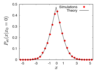
Figure 2: Theory versus simulation results for the stationary spatial distribution of a free Brownian particle undergoing parabolic resetting. The points denote simulation results, while the line stands for the exact analytical expression given in Eq. (58). The numerical results were obtained from $10^{4}$ independent simulations of the Langevin dynamics described in Section II.1. The error bars associated with the data points are smaller than the symbol size. The parameter values are $D=1.0,\alpha=0.5$.

The result (58) is checked in simulations in Fig. 2. The simulations involved numerically integrating the dynamics described in Section II.1, with integration timestep equal to $0.01$. Using $\int_{0}^{\infty}{\rm d}t~{}t^{\mu-1}K_{\nu}(t)=2^{\mu-2}\Gamma\Big{(}\frac{\mu}{2}-\frac{\nu}{2}\Big{)}\Gamma\Big{(}\frac{\mu}{2}+\frac{\nu}{2}\Big{)}$ for $|{\rm Re}~{}\nu|<|{\rm Re}~{}\mu|$ Olver:2016 , we find that $P_{\rm st}(x|x_{0}=0)$ given by Eq. (58) is correctly normalized to unity. Moreover, using the results that as $x\to 0$, we have $K_{\nu}(x)=\frac{\Gamma(\nu)}{2}\Big{(}\frac{x}{2}\Big{)}^{-\nu}$ for ${\rm Re}~{}\nu>0$ and that as $x\to\infty$, we have $K_{\nu}(x)=\Big{(}\frac{\pi}{2x}\Big{)}^{1/2}\exp(-x)$ for real $x$ Olver:2016 , we get

$$P_{\rm st}(x|x_{0}=0)\sim\left\{\begin{array}[]{ll}\frac{(\alpha/D)^{1/4}}{\sqrt{\pi}}&~{}~{}{\rm for}~{}~{}x\to 0,\\ \exp(-x^{2}\sqrt{\alpha/D}/2)&~{}~{}{\rm for}~{}~{}|x|\to\infty.\\ \end{array}\right.$$ (62)

Using Eq. (58) and the result ${\rm d}K_{1/4}(x)/{\rm d}x=-(1/2)\left(K_{3/4}(x)+K_{5/4}(x)\right)$, it may be easily shown that as $x\to 0^{\pm}$, one has ${\rm d}P_{\rm st}(x|x_{0}=0))/{\rm d}x=\mp\sqrt{\alpha/D}\Gamma(3/4)/(\sqrt{\pi}\Gamma(1/4))$, implying thereby that the first derivative of $P_{\rm st}(x|x_{0}=0)$ is discontinuous at $x=0$. We thus conclude that the spatial distribution $P_{\rm st}(x|x_{0}=0)$ exhibits a cusp singularity at $x=0$. This feature of cusp singularity at the resetting location $x_{0}=0$ is also seen in the stationary distribution (45), and is a signature of the steady state being a nonequilibrium one Evans:2011-1 ; Gupta:2014 ; Nagar:2016 ; Gupta:2016 . Note the existence of faster-than-exponential tails suggested by Eq. (62) in comparison to the exponential tails observed in the case of resetting at a constant rate, see Eq. (45). This is consistent with the fact that with respect to the case of resetting at a space-independent rate, a parabolic rate of resetting implies that the further the particle is from $x_{0}=0$, the more enhanced is the probability that a resetting event takes place, and, hence, a smaller probability of finding the particle far away from the resetting location.

Let us consider the case of an overdamped Brownian particle that is trapped in a harmonic potential $V(x)=(1/2)\kappa x^{2}$, with $\kappa>0$, and is undergoing the Langevin dynamics (1). At equilibrium, the distribution of the position of the particle is given by the Boltzmann-Gibbs distribution

$$P_{\rm eq}(x) = \exp(-\kappa x^{2}/2k_{\rm B}T)/Z,$$ (63)

with $Z=\sqrt{2\pi k_{\rm B}T/\kappa}$ being the partition function. Comparing Eqs. (62) and (63), we see that using a harmonic potential with a suitable $\kappa$, the stationary distribution of a free Brownian particle undergoing parabolic resetting may be made to match in the tails with the stationary distribution of a Brownian particle trapped in the harmonic potential and evolving in the absence of any resetting. On the other hand, the cusp singularity in the former cannot be achieved with the Langevin dynamics in any harmonic potential without the inclusion of resetting events.

Let us note that the stationary states (45) and (58) are entirely induced by the dynamics of resetting. Indeed, in the absence of any resetting, the dynamics of a free diffusing particle does not allow for a long-time stationary state, since in the absence of a force, there is no way in which the motion of the particle can be bounded in space. On the other hand, in presence of resetting, the dynamics of repeated relocation to a given position in space can effectively compete with the inherent tendency of the particle to spread out in space, leading to a bounded motion, and, hence, a relaxation to a stationary spatial distribution at long times. In the next section, we consider the situation where the particle even in the absence of any resetting has a localized stationary spatial distribution, and investigate the change in the nature of the spatial distribution of the particle owing to the inclusion of resetting events.

III.3 Particle trapped in a harmonic potential with energy-dependent resetting

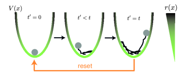
Figure 3: Illustration of the energy-dependent resetting of a Brownian particle moving in a harmonic potential. A Brownian particle (grey circle) immersed in a thermal bath at temperature $T$ moves with diffusion coefficient $D$, with its motion being confined by a harmonic potential $V(x)=\kappa x^{2}/2$ (green), with $\kappa$ being the stiffness constant. Here, $x$ is the position of the particle with respect to the center of the potential. The particle, initially located in the trap center ($t^{\prime}=0$, left panel), diffuses at subsequent times in the energy landscape ($t^{\prime}<t$, middle panel), until a resetting event occurs at time $t^{\prime}=t$ (right panel). The black curve represents the history of the particle from $t^{\prime}=0$ up to the time corresponding to each snapshot. The rate of resetting (right colorbar) is proportional to the instantaneous energy of the particle, and, therefore, a reset is more likely to take place as the particle climbs up the potential.

We now introduce a resetting problem that is relevant in physics: an overdamped Brownian particle immersed in a thermal bath at temperature $T$ and trapped with a harmonic potential centered at the origin: $V(x)=(1/2)\kappa x^{2}$, where $\kappa>0$ is the stiffness constant of the harmonic potential. The particle, initially located at $x_{0}=0$, may be reset at any time $t$ to the origin with a probability that depends on the energy of the particle at time $t$. The dynamics is shown schematically in Fig. 3. For purposes of illustration of the nontrivial effects of resetting, we consider the following space-dependent reseting rate:

$$r(x)=\frac{3}{2\tau_{c}}\frac{V(x)}{k_{\rm B}T}=\frac{3}{4}\frac{\mu^{2}\kappa^{2}}{D}x^{2},$$ (64)

where we use $D=k_{B}T\mu$ in obtaining the second equality. Note that the resetting rate is proportional to the energy of the particle (in units of $k_{\rm B}T$) divided by the timescale $\tau_{c}\equiv 1/\mu\kappa$ that characterizes the relaxation of the particle in the harmonic potential in the absence of any resetting. In this way, it is ensured that the rate of resetting (64) has units of inverse time. Note also that in the absence of any resetting, the particle relaxes to an equilibrium stationary state with a spatial distribution given by the usual Boltzmann-Gibbs form:

$$P_{\rm st}^{r(x)=0}(x)=\sqrt{\frac{\kappa}{2\pi k_{B}T}}\exp\left(-\frac{\kappa x^{2}}{2k_{B}T}\right).$$ (65)

Using $F(x)=-\partial_{x}V(x)=-\kappa x$ and the expression (64) for the resetting rate in Eq. (21), we find that the potential of the corresponding quantum mechanical problem is given by

$$V_{\rm q}(x)=\frac{\mu^{2}(F(x))^{2}}{4D}+\frac{\mu F^{\prime}(x)}{2}+r(x)=\frac{\mu^{2}\kappa^{2}x^{2}}{D}-\frac{\mu\kappa}{2},$$ (66)

where we have used $F^{\prime}(x)=-\kappa$. From Eqs. (17) and (18), we obtain

$$P_{\rm no\;res}(x,t|x_{0}=0,0)=\exp\left(\frac{\mu}{2D}\int_{x_{0}}^{x}F(x)~{}{\rm d}x\right)$$

$$\times\exp\left(\frac{\mu\kappa t}{2}\right)\langle x|\exp(-H_{\rm q}t)|x_{0}=0\rangle$$

$$=\exp\left(-\frac{x^{2}}{4D\tau_{c}}\right)\exp\left(\frac{t}{2\tau_{c}}\right)\langle x|\exp(-H_{\rm q}t)|x_{0}=0\rangle,$$

(67)

where the quantum Hamiltonian is given by

$$H_{\rm q}=-\frac{1}{2m_{\rm q}}\frac{\partial^{2}}{\partial x^{2}}+\frac{\mu^{2}\kappa^{2}x^{2}}{D};~{}~{}m_{\rm q}=\frac{1}{2D},~{}\hbar=1.$$ (68)

We thus find that the propagator $\langle x|\exp(-H_{\rm q}t)|x_{0}=0\rangle$ is given by the propagator of a quantum harmonic oscillator, which has been calculated in Sec. III.2. In fact, the Hamiltonian given by Eq. (68) is identical to that in Eq. (48) with the identification $\alpha=\mu^{2}\kappa^{2}/D=1/D\tau_{c}^{2}$, so that by substituting $x_{0}=0$ and $\alpha=1/(D\tau_{c}^{2})$ in Eq. (52), we obtain

$$\langle x|\exp(-H_{\rm q}t)|x_{0}=0\rangle=$$

$$\frac{1}{\sqrt{2\pi D\tau_{c}\sinh(2t/\tau_{c})}}\exp\left(-\frac{x^{2}}{2D\tau_{c}}\coth(2t/\tau_{c})\right).$$

From Eqs. (67) and (III.3), we obtain

$$P_{\rm no\;res}(x,t|x_{0}=0,0)=$$

$$\frac{\exp(t/2\tau_{c})}{\sqrt{2\pi D\tau_{c}\sinh(2t/\tau_{c})}}\exp\left(-\frac{x^{2}}{2D\tau_{c}}\left[\frac{1}{2}+\coth(2t/\tau_{c})\right]\right).$$

(70)

Following Eq. (22), we may now calculate the probability of the first-reset time by using Eq. (70) to get

$$P_{\rm res}(t|x_{0}=0)=\frac{\exp(t/2\tau_{c})}{\sqrt{2\pi D\tau_{c}\sinh(2t/\tau_{c})}}$$

$$\times\int_{-\infty}^{\infty}{\rm d}x\frac{3x^{2}}{4D\tau_{c}^{2}}\exp\left(-\frac{x^{2}}{2D\tau_{c}}\left[\frac{1}{2}+\coth(2t/\tau_{c})\right]\right)$$

$$=\frac{3\exp(t/2\tau_{c})}{4\tau_{c}}\sqrt{\frac{1}{\sinh(2t/\tau_{c})(1/2+\coth(2t/\tau_{c}))^{3}}},$$

which may be checked to be normalized: $\int_{0}^{\infty}{\rm d}t~{}P_{\rm res}(t|x_{0}=0)=1$. The first-reset time distribution (III.3) may be written in the scaling form

$$P_{\rm res}(t|x_{0}=0) = \frac{3}{4\tau_{c}}{\cal G}\!\left(\frac{2t}{\tau_{c}}\right),$$ (72)

with the scaling function given by ${\cal G}(y)=\exp(y/4)\sinh(y)^{-1/2}(1/2+\coth(y))^{-3/2}$.

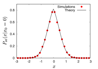
Figure 4: Theory versus simulation results for the stationary spatial distribution of a Brownian particle trapped in a harmonic potential and undergoing energy-dependent resetting. The points denote simulation results, while the line stands for the exact analytical expression given in Eq. (75). The numerical results were obtained from $10^{4}$ independent simulations of the Langevin dynamics described in Section II.1. The error bars associated with the data points are smaller than the symbol size. The parameter values are $D=1.0,\tau_{c}=0.5$.

The mean first-reset time, given by $\langle t\rangle_{\rm res}\equiv\int_{0}^{\infty}{\rm d}tP_{\rm res}(t|x_{0}=0)$, equals

$$\langle t\rangle_{\rm res}=\frac{4\tau_{c}}{\sqrt{3}}\,_{2}F_{1}\!\left(\frac{1}{8},\frac{1}{2};\frac{9}{8};-\frac{1}{3}\right),$$ (73)

where ${}_{p}F_{q}(a_{1},a_{2},\ldots,a_{p};b_{1},b_{2},\ldots,b_{q};x)$ is the generalized hypergeometric function. Introducing the variable $z\equiv 2t/\tau_{c}$, and using Eq. (70), we get

$$P_{\rm st}(x|x_{0}=0)=\frac{1}{\langle t\rangle_{\rm res}}\sqrt{\frac{\tau_{c}}{8\pi D}}\exp\left(-\frac{x^{2}}{4D\tau_{c}}\right)$$

$$\times\int_{0}^{\infty}{\rm d}z\frac{\exp(z/4)}{\sqrt{\sinh(z)}}\exp\left(-\frac{x^{2}\coth z}{2D\tau_{c}}\right)$$

$$=\frac{1}{\langle t\rangle_{\rm res}}\sqrt{\frac{\tau_{c}}{8\pi D}}\exp\left(-\frac{x^{2}}{4D\tau_{c}}\right)$$

$$\times\frac{1}{2}\left(\frac{x^{2}}{4D\tau_{c}}\right)^{-1/4}\Gamma(1/8)\,W_{1/8,1/4}\left(\frac{x^{2}}{D\tau_{c}}\right),$$ (74)

where $W_{\mu,\nu}$ is Whittaker’s W function.

Using Eq. (73) in Eq. (74), we obtain

$$P_{\rm st}(x|x_{0}=0)=\frac{(1/8)\Gamma(1/8)}{\,{}_{2}F_{1}\!\left(\frac{1}{8},\frac{1}{2};\frac{9}{8};-\frac{1}{3}\right)}$$

$$\times\sqrt{\frac{3}{8\pi D\tau_{c}}}\exp\left(-\frac{x^{2}}{4D\tau_{c}}\right)\left(\frac{4D\tau_{c}}{x^{2}}\right)^{1/4}\,W_{1/8,1/4}\left(\frac{x^{2}}{D\tau_{c}}\right),$$

(75)

which may be checked to be normalized to unity. We may write the stationary distribution in terms of a scaled position variable as

$$P_{\rm st}(x|x_{0}=0)=\frac{(1/8)\Gamma(1/8)}{\,{}_{2}F_{1}\!\left(\frac{1}{8},\frac{1}{2};\frac{9}{8};-\frac{1}{3}\right)}\sqrt{\frac{3}{8\pi D\tau_{c}}}\mathcal{R}\!\left(\frac{x}{\sqrt{2D\tau_{c}}}\right),$$

(76)

with $\mathcal{R}(y)\equiv\exp(-y^{2}/2)(2/y^{2})^{1/4}\,W_{1/8,1/4}(2y^{2})$ being the scaling function. The expression (75) is checked in simulations in Fig. 4. The simulations involved numerically integrating the dynamics described in Section II.1, with integration timestep equal to $0.01$. Using the results that as $x\to 0$, we have $W_{k,\mu}(x)=\frac{\Gamma(2\mu)}{\Gamma(1/2+\mu-k)}x^{1/2-\mu}$ for $0\leq{\rm Re}~{}\mu<1/2,~{}\mu\neq 0$ and that as $x\to\infty$, we have $W_{k,\mu}(x)\sim e^{-x/2}x^{k}$ for real $x$ Olver:2016 , we get

$$P_{\rm st}(x|x_{0}=0)\sim\left\{\begin{array}[]{ll}\frac{(1/8)\Gamma(1/8)}{\thinspace{}_{2}F_{1}(1/8,1/2;9/8;-1/3)}\thinspace\frac{\sqrt{3/8D\tau_{c}}}{\Gamma(5/8)}&{\rm for}~{}x\to 0,\\ \exp\Big{(}-\frac{3x^{2}}{4D\tau_{c}}\Big{)}&{\rm for}~{}|x|\to\infty.\\ \end{array}\right.$$

We see again the existence of a cusp at the resetting location $x_{0}=0$, similar to all other cases we studied in this paper.

The results of this subsection could inspire future experimental studies using optical tweezers in which the resetting protocol could be effectively implemented by using feedback control Berut:2012 ; Roldan:2014 ; Koski:2014 . Interestingly, colloidal and molecular gelly and glassy systems show hopping motion of their constituent particles between potential traps or “cages,” the latter originating from the interaction of the particles with their neighbors Sandalo:2017 . Such a phenomenon is also exhibited by out-of-equilibrium glasses and gels during the process of aging Ludovic:2011 . Our results in this section could provide valuable insights into the aforementioned dynamics, since the emergent potential cages may be well approximated by harmonic traps and the hopping process as a resetting event.

IV Shortcuts to confinement

A hallmark of the examples solved exactly in Sec. III by using our path-integral formalism is the existence of stationary distributions with prominent cusp singularities (see Figs. 2 and 4). These examples demonstrate that the particle can be confined around a prescribed location by using appropriate space-dependent rates of resetting.

In physics and nanotechnology, the issue of achieving an accurate control of fluctuations of small-sized particles is nowadays attracting considerable attention Martinez:2013 ; Berut:2014 ; Dieterich:2015 . For instance, using optical tweezers and noisy electrostatic fields, it is now possible to control accurately the amplitude of fluctuations of the position of a Brownian particle Martinez:2017 ; Gavrilov:2017 ; Ciliberto:2017 . Such fluctuations may be characterized by an effective temperature. Experiments have reported effective temperatures of a colloidal particle in water up to 3000K Martinez:2013 , and have recently been used to design colloidal heat engines at the mesoscopic scale Martinez:2016 ; Martinez:2017 . Effective confinement of small systems is of paramount importance for success of quantum-based computations with, e.g., cold atoms Cirac:1995 ; Bloch:2005 .

Does stochastic resetting provide an efficient way to reduce the amplitude of fluctuations of a Brownian particle, thereby providing a technique to reduce the associated effective temperature? We now provide some insights into this question.

Consider the following example of a nonequilibrium protocol: i) a Brownian particle is initially confined in a harmonic trap with a potential $V(x)=(1/2)\kappa x^{2}$ for a sufficiently long time such that it is in an equilibrium state with spatial distribution $P_{\rm eq}(x)=\exp(-\kappa x^{2}/2k_{\rm B}T)/Z$, with $Z=\sqrt{2\pi k_{\rm B}T/\kappa}$; ii) a space-dependent (parabolic) resetting rate $r(x)=(3/2\tau_{c})V(x)/k_{\rm B}T$, with $\tau_{c}=(1/\mu\kappa)$, is suddenly switched on by an external agent. In order words, the rate of resetting is instantaneously quenched from $r(x)=0$ to $r(x)=(3/4)(\mu^{2}\kappa^{2}/D)x^{2}$; iii) the particle is let to relax to a new stationary state in the presence of the trapping potential and parabolic resetting. At the end of the protocol, the particle relaxes to the stationary distribution $P_{\rm st}(x)$ given by Eq. (76).

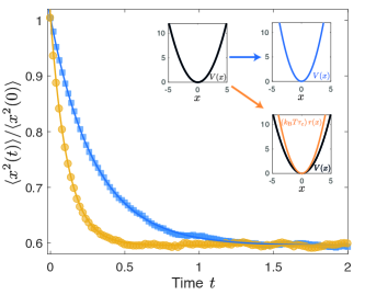
Figure 5: Shortcut to particle confinement. Confinement of a Brownian particle using harmonic potentials and space-dependent rates of resetting. The symbols represent simulation results for relaxation processes of $10^{5}$ non-interacting Brownian particles that are initially in equilibrium in a harmonic potential $V(x)=(1/2)\kappa x^{2}$. The blue circles represent the mean-squared displacement of the particle in units of $\langle x^{2}(0)\rangle$ after an instantaneous quench to a harmonic potential with stiffness $\kappa^{\prime}=1.7\kappa$ (the blue arrow in the inset). The yellow circles on the other hand represent the mean-squared displacement of the particle in units of $\langle x^{2}(0)\rangle$ after an instantaneous quench of the rate of resetting from $r(x)=0$ to $r(x)=(3/4)(\mu^{2}\kappa^{2}/D)x^{2}$ (the orange arrow in the inset). For the case in which the stiffness of the potential is quenched from $\kappa$ to $\kappa^{\prime}$, it is easily seen that $\langle x^{2}(t)\rangle=\langle x^{2}(0)\rangle\exp(-2\mu k^{\prime}t)+(D/(\mu k^{\prime}))[1-\exp(-2\mu k^{\prime}t)]$, thereby implying a relaxation timescale $\tau_{\rm quench}=1/(2\mu k^{\prime})$ and yielding the corresponding curve in the figure. Note that the time in the $x$-axis is measured in units of $\tau_{c}=1/\mu\kappa$. The other curve depicting the process of relaxation in presence of resetting may be fitted to a good approximation to $A+Be^{-t/\tau_{\rm reset}}$. One observes that $\tau_{\rm reset}\approx\tau_{\rm quench}/3$. The parameter values are $D=1$, $\kappa=1$ and $\mu=10$.

We first note that before the sudden switching on of the resetting dynamics, which we assume to happen at a reference time instant $t=0$, the mean-squared displacement of the particle is given by

$$\langle x^{2}(0)\rangle=\frac{k_{\rm B}T}{\kappa},$$ (79)

which follows from the equilibrium distribution before the resetting is switched on, and is in agreement with the equipartition theorem $\kappa\langle x^{2}(0)\rangle/2=k_{\rm B}T/2$. After the sudden switching on of the space-dependent rate of resetting, the variance of the position of the particle relaxes at long times to the stationary value

$$\langle x^{2}(\infty)\rangle=\frac{k_{\rm B}T/\kappa}{\sqrt{3}\,_{2}F_{1}\!\left(\frac{1}{8},\frac{1}{2};\frac{9}{8};-\frac{1}{3}\right)}\simeq 0.59\frac{k_{\rm B}T}{\kappa},$$ (80)

as follows from Eq. (76). The resetting dynamics induces in this case a reduction by about $40\%$ of the variance of the position of the particle with respect to its initial value. We note that such a reduction of the amplitude of fluctuations of the particle could also have been achieved by performing a sudden quench of the stiffness of the harmonic potential by increasing its value from $\kappa$ to $\kappa^{\prime}\simeq(1/0.59)\kappa\simeq 1.7\kappa$, without the need for switching on of resetting events. To understand the difference between the two scenarios, it is instructive to compare the time evolution of the mean-squared displacement $\langle x^{2}(t)\rangle$ towards the stationary value in the two cases, see inset in Fig. 5. We observe that resetting leads to the same degree of confinement in a shorter time. For the case in which the stiffness of the potential is quenched from $\kappa$ to $\kappa^{\prime}$, it is easily seen that $\langle x^{2}(t)\rangle=\langle x^{2}(0)\rangle\exp(-2\mu k^{\prime}t)+(D/(\mu k^{\prime}))[1-\exp(-2\mu k^{\prime}t)]$, thereby implying a relaxation timescale $\tau_{\rm quench}=1/(2\mu k^{\prime})$ and yielding the corresponding curve in Fig. 5. The other curve depicting the process of relaxation in presence of resetting may be fitted to a good approximation to $A+Be^{-t/\tau_{\rm reset}}$. One observes that $\tau_{\rm reset}\approx\tau_{\rm quench}/3$. Thus, for the example at hand, we may conclude that a sudden quench of resetting profiles provides a shortcut to confinement of the position of the particle to a desired degree with respect to a potential quench. Similar conclusions were arrived at for mean first-passage times of resetting processes and equivalent equilibrium dynamics Evans:2013 .

It may be noted that the confinement protocol by a sudden quench of resetting profiles introduced above is amenable to experimental realization. Using microscopic particles trapped with optical tweezers Martinez:2017 ; Ciliberto:2017 or feedback traps Jun:2012 ; Gavrilov:2017 ; Gavrilov:2014 , it is now possible to measure and control the position of a Brownian particle with subnanometric precision. Recent experimental setups allow to exert random forces to trapped particles, with a user-defined statistics for the random force Martinez:2013 ; Berut:2014 ; Martinez:2014 ; Martinez:2017 . The shortcut protocol using resetting could be explored in the laboratory by designing a feedback-controlled experiment with optical tweezers and by employing random-force generators according to, e.g., the protocol sketched in Fig. 3.

V Conclusions and outlook

In this paper, we addressed the fundamental question of what happens when a continuously evolving stochastic process is repeatedly interrupted at random times by a sudden reset of the state of the process to a given fixed state. To this end, we studied the dynamics of an overdamped Brownian particle diffusing in force fields and resetting to a given spatial location with a rate that has an essential dependence on space, namely, the probability with which the particle resets is a function of the current location of the particle.

To address stochastic resetting in the aforementioned scenario, we employed a path-integral approach, discussed in detail in Eqs. (17)-(21) in Sec. II.2.1. Invoking the Feynman-Kac formalism, we obtained an equality that relates the probability of transition between different spatial locations of the particle before it encounters any reset to the quantum propagator of a suitable quantum mechanical problem (see Sec. II.2.1). Using this formalism and elements from renewal theory, we obtained closed-form analytical expressions for a number of statistics of the dynamics, e.g., the probability distribution of the first-reset time (Sec. II.2.2), the time-dependent spatial distribution (Sec. II.2.3), and the stationary spatial distribution (Sec. II.2.4).

We applied the method to a number of representative examples, including in particular those involving nontrivial spatial dependence of the rate of resetting. Remarkably, we obtained the exact distributions of the aforementioned dynamical quantifiers for two non-trivial problems: the resetting of a free Brownian particle under “parabolic” resetting (Sec. III.2) and the resetting of a Brownian particle moving in a harmonic potential with a resetting rate that depends on the energy of the particle (Sec. III.3). For the latter case, we showed that using instantaneous quenching of resetting profiles allows to restrict the mean-squared displacement of a Brownian particle to a desired value on a faster timescale than by using instantaneous potential quenches. We expect that such a shortcut to confinement would provide novel insights in ongoing research on, e.g., engineered-swift-equilibration protocols ESE ; Granger:2016 and shortcuts to adiabaticity Deffner:2013 ; Deng:2013 ; Tu:2014 .

Our work may also be extended to treat systems of interacting particles, with the advantage that the corresponding quantum mechanical system can be treated effectively by using tools of quantum physics and many-body quantum theory. Our approach also provides a viable method to calculate path probabilities of complex stochastic processes. Such calculations are of particular interest in many contexts, e.g., in stochastic thermodynamics Jarzynski:2011 ; Seifert:2012 ; Celani:2012 ; Bo:2017 , and in the study of several biological systems such as molecular motors Julicher:1997 ; Guerin:2011 , active gels Basu:2008 , genetic switches Perez-Carrasco:2016 ; Schultz:2008 , etc. As a specific application in this direction, our approach allows to explore the physics of Brownian tunnelling Roldan , an interesting stochastic resetting version of the well-known phenomenon of quantum tunneling, which serves to unveil the subtle effects resulting from stochastic resetting in, e.g., transport through nanopores Trepagnier:2007 .

VI Acknowledgements

ER thanks Ana Lisica and Stephan Grill for initial discussions, Ken Sekimoto and Luca Peliti for discussions on path integrals, and Domingo Sánchez and Juan M. Torres for discussions on quantum mechanics.

References

- (1) Landauer R 1961 Irreversibility and heat generation in the computing process IBM J. Res. Develop. 5 183
- (2) Bennett C H 1973 Logical reversibility of computation IBM J. Res. Develop. 17 525
- (3) Bérut A, Arakelyan A, Petrosyan A, Ciliberto S, Dillenschneider R, and Lutz E 2012 Experimental verification of Landauer’s principle linking information and thermodynamics Nature 483 187
- (4) Mandal D and Jarzynski C 2012 Work and information processing in a solvable model of Maxwell’s demon Proc. Natl. Acad. Sci. 109 11641
- (5) Roldán É, Martínez I A, Parrondo J M R, and Petrov D 2014 Universal features in the energetics of symmetry breaking Nature Phys. 10 457
- (6) Koski J V, Maisi V F, Pekola J P, and Averin D V 2014 Experimental realization of a Szilard engine with a single electron Proc. Natl. Acad. Sci. 111 13786
- (7) Fuchs J, Goldt G, and Seifert U 2016 Stochastic thermodynamics of resetting Europhys. Lett. 113 60009
- (8) Mora T 2015 Physical Limit to Concentration Sensing Amid Spurious Ligands Phys. Rev. Lett. 115 038102
- (9) Roldán É, Lisica A, Sánchez-Taltavull D, Grill S W 2016 Stochastic resetting in backtrack recovery by RNA polymerases Phys. Rev. E 93 062411
- (10) Lisica A, Engel C, Jahnel M, Roldán É, Galburt E A, Cramer P, and Grill S W 2016 Mechanisms of backtrack recovery by RNA polymerases I and II Proc. Natl. Acad. Sci. USA 113 2946
- (11) Gillespie D T, Seitaridou E, and Gillespie C A 2014 The small-voxel tracking algorithm for simulating chemical reactions among diffusing molecules J. Chem. Phys. 141 12649
- (12) Hanggi P, Talkner P, and Borkovec M 1990 Reaction-rate theory: fifty years after Kramers Rev. Mod. Phys. 62 251
- (13) Neri I, Roldán É, and Jülicher F 2017 Statistics of Infima and Stopping Times of Entropy production and Applications to Active Molecular Processes Phys. Rev. X 7 011019
- (14) Jülicher F, Ajdari A, and Prost J 1997 Modeling molecular motors Rev. Mod. Phys. 69 1269
- (15) Zamft B, Bintu L, Ishibashi T, and Bustamante C J 2012 Nascent RNA structure modulates the transcriptional dynamics of RNA polymerases Proc. Natl. Acad. Sci. 109 8948
- (16) Evans M R and Majumdar S N 2011 Diffusion with stochastic resetting Phys. Rev. Lett. 106 160601
- (17) Evans M R and Majumdar S N 2011 Diffusion with optimal resetting J. Phys. A: Math. Theor. 44 435001
- (18) Evans M R and Majumdar S N 2014 Diffusion with resetting in arbitrary spatial dimension J. Phys. A: Math. Theor. 47 285001
- (19) Christou C and Schadschneider A 2015 Diffusion with resetting in bounded domains J. Phys. A: Math. Theor. 48 285003
- (20) Eule S and Metzger J J 2016 Non-equilibrium steady states of stochastic processes with intermittent resetting New J. Phys. 18 033006
- (21) Nagar A and Gupta S 2016 Diffusion with stochastic resetting at power-law times Phys. Rev. E 93 060102(R)
- (22) Boyer D and Solis-Salas C 2014 Random walks with preferential relocations to places visited in the past and their application to biology Phys. Rev. Lett. 112 240601
- (23) Majumdar S N, Sabhapandit S, and Schehr G 2015 Random walk with random resetting to the maximum position Phys. Rev. E 92 052126
- (24) Montero M and Villarroel J 2013 Monotonic continuous-time random walks with drift and stochastic reset events Miquel Montero Phys. Rev. E 87 012116
- (25) Méndez V and Campos D 2016 Characterization of stationary states in random walks with stochastic resetting Phys. Rev. E 93 022106
- (26) Kuśmierz L, Majumdar S N, Sabhapandit S, and Schehr G 2014 First order transition for the optimal search time of Lévy flights with resetting Phys. Rev. Lett. 113 220602
- (27) Campos D and Méndez V 2015 Phase transitions in optimal search times: How random walkers should combine resetting and flight scales Phys. Rev. E 92 062115
- (28) Pal A, Kundu A, and Evans M R 2016 Diffusion under time-dependent resetting J. Phys. A: Math. Theor. 49 225001
- (29) Boyer D, Evans M R, and Majumdar S N 2017 Long time scaling behaviour for diffusion with resetting and memory J. Stat. Mech.: Theory Exp. 023208
- (30) Harris R J and Touchette H 2017 Phase transitions in large deviations of reset processes J. Phys. A: Math. Theor. 50 10LT01
- (31) Durang X, Henkel M, and Park H 2014 The statistical mechanics of the coagulation–diffusion process with a stochastic reset J. Phys. A: Math. Theor. 47 045002
- (32) Gupta S, Majumdar S N, and Schehr G 2014 Fluctuating interfaces subject to stochastic resetting Phys. Rev. Lett. 112 220601
- (33) Gupta S and Nagar A 2016 Resetting of fluctuating interfaces at power-law times J. Phys. A: Math. Theor. 49 445001
- (34) Falcao R and Evans M R 2017 Interacting Brownian motion with resetting J. Stat. Mech.: Theory Exp. 023204
- (35) Kuśmierz L and Gudowska-Nowak E 2015 Optimal first-arrival times in Lévy flights with resetting Phys. Rev. E 92 052127
- (36) Reuveni S 2016 Optimal stochastic restart renders fluctuations in first passage times universal Phys. Rev. Lett. 116 170601
- (37) Bhat U, De Bacco C, and Redner S 2016 Stochastic search with Poisson and deterministic resetting J. Stat. Mech.: Theory Exp. 083401
- (38) Pal A and Reuveni S 2017 First passage under restart Phys. Rev. Lett. 118 030603
- (39) Pal A 2015 Diffusion in a potential landscape with stochastic resetting Phys. Rev. E 91 012113
- (40) Cox D 1962 Renewal Theory (London: Methuen)
- (41) Feynman R P and Hibbs A R 2010 Quantum Mechanics and Path Integrals (New York: McGraw-Hill Companies, Inc.)
- (42) Schulman L S 1981 Techniques and Applications of Path Integration (UK: John Wiley & Sons)
- (43) Kac M 1949 On distribution of certain Wiener functionals Trans. Am. Math. Soc. 65 1
- (44) Kac M 1951 On some connections between probability theory and differential and integral equations, in Proc. Second Berkeley Symp. on Math. Statist. and Prob. (Berkeley: University of California Press)
- (45) Majumdar S N 2005 Brownian Functionals in Physics and Computer Science Curr. Sci. 89 2076
- (46) In quantum mechanics, this time transformation is often called the Wick’s rotation in honor of Gian-Carlo Wick
- (47) Sekimoto K 1998 Langevin equation and thermodynamics Prog. Theor. Phys. Suppl. 130 17
- (48) Sekimoto K 2000 Stochastic Energetics (Berlin: Springer)
- (49) Olver F W J, Daalhuis A B O, Lozier D W, Schneider B I, Boisvert R F, Clark C W, Miller B R, and Saunders B V eds. NIST Digital Library of Mathematical Functions, http://dlmf.nist.gov/, Release 1.0.14 of 2016-12-21
- (50) Roldán-Vargas S, Rovigatti L, and Sciortino F 2017 Connectivity, dynamics, and structure in a tetrahedral network liquid Soft Matter 13 514
- (51) Berthier L, and Biroli G 2011 Theoretical perspective on the glass transition and amorphous materials Rev. Mod. Phys. 83 587
- (52) Martínez I A, Roldán É, Parrondo J M R, and Petrov D 2013 Effective heating to several thousand kelvins of an optically trapped sphere in a liquid Phys. Rev. E 87 032159
- (53) Bérut A, Petrosyan A, and Ciliberto S 2015 Energy flow between two hydrodynamically coupled particles kept at different effective temperatures EPL (Europhys. Lett.) 107 (6) 60004.
- (54) Dieterich E., Camunas-Soler J., Ribezzi-Crivellari M., Seifert U, and Ritort, F 2015 Single-molecule measurement of the effective temperature in non-equilibrium steady states Nature Phys. 11 (11), 97
- (55) Martínez I A, Roldán É, Dinis L and Rica R A 2017 Colloidal heat engines: a review Soft matter 13 (1) 22.
- (56) Cirac J I, and Zoller P 1995 Quantum computations with cold trapped ions Phys. Rev. Lett. 74 (20) 4091.
- (57) Bloch I 2005 Ultracold quantum gases in optical lattices Nature Phys. 1 (1) 23.
- (58) Gavrilov M, Chétrite R and Bechhoefer J 2017 Direct measurement of nonequilibrium system entropy is consistent with Gibbs-Shannon form arXiv preprint arXiv:1703.07601.
- (59) Ciliberto S 2017 Experiments in Stochastic Thermodynamics: Short History and Perspectives Phys. Rev. X 7 021051.
- (60) Martínez I A, Roldán É, Dinis L, Petrov D, Parrondo J M R, and Rica R A 2016 Brownian carnot engine Nature Phys. 12 (1) 67.
- (61) Evans M R, Majumdar S N and Mallick K 2013 Optimal diffusive search: nonequilibrium resetting versus equilibrium dynamics J. Phys. A 46 (18) 185001.
- (62) Gavrilov M, Jun Y and Bechhoefer J, 2014 Real-time calibration of a feedback trap Rev. Sci. Instr. 85 (9) 095102.
- (63) Jun Y and Bechhoefer J 2012.Virtual potentials for feedback traps Phys. Rev. E 86 (6) 061106.
- (64) Martínez I A, Roldán É, Dinis L, Petrov D and Rica R A 2015 Adiabatic processes realized with a trapped Brownian particle Phys. Rev. Lett. 114 (12) 120601.
- (65) Martínez I A, Petrosyan A, Guéry-Odelin D, Trizac E and Ciliberto S 2016 Engineered swift equilibration of a Brownian particle Nature Phys. 12 (9) 843.
- (66) Granger L, Dinis L, Horowitz J M and Parrondo J M R 2016. Reversible feedback confinement EPL (Europhys. Lett.) 115 (5) 50007.
- (67) Deffner S, Jarzynski C and del Campo A 2014 Classical and quantum shortcuts to adiabaticity for scale-invariant driving Phys. Rev. X 4 (2) 021013.
- (68) Deng J, Wang Q H, Liu Z, Hänggi P and Gong J 2013. Boosting work characteristics and overall heat-engine performance via shortcuts to adiabaticity: Quantum and classical systems Phys. Rev. E 88 (6) 062122.
- (69) Tu Z C 2014 Stochastic heat engine with the consideration of inertial effects and shortcuts to adiabaticity Phys. Rev. E 89 (5) 052148.
- (70) Jarzynski C 2011 Equalities and inequalities: irreversibility and the second law of thermodynamics at the nanoscale Annu. Rev. Condens. Matt. Phys. 2 329
- (71) Seifert U 2012 Stochastic thermodynamics, fluctuation theorems and molecular machines Rep. Prog. Phys. 75 12
- (72) Celani A, Bo S, Eichhorn R and Aurell E 2012 Anomalous thermodynamics at the microscale Phys. Rev. Lett. 109 (26) 260603.
- (73) Bo S and Celani A 2017 Stochastic processes on multiple scales: averaging, decimation and beyond Bull. Am. Phys. Soc. 62 1.
- (74) Guérin T, Prost J, and Joanny J-F 2011 Motion reversal of molecular motor assemblies due to weak noise Phys. Rev. Lett. 106 068101
- (75) Basu A, Joanny J-F, Jülicher F, and Prost J 2008 Thermal and non-thermal fluctuations in active polar gels Eur. Phys. J. E 27 149
- (76) Perez-Carrasco R, Guerrero P, Briscoe J, and Page KM 2016 Intrinsic noise profoundly alters the dynamics and steady state of morphogen-controlled bistable genetic switches PLoS Comput. Biol. 12 e1005154
- (77) Schultz D, Walczak A M, Onuchic J N, Wolynes P G 2008 Extinction and resurrection in gene networks Proc. Natl. Acad. Sci. 105 19165
- (78) Roldán E and Gupta S (in preparation)
- (79) Trepagnier E H, Radenovic A, Sivak D, Geissler P, and Liphardt L 2007 Controlling DNA capture and propagation through artificial nanopores Nano Lett. 7 2824