Bright and Gap Solitons in Membrane-Type Acoustic Metamaterials

Abstract

We study analytically and numerically envelope solitons (bright and gap solitons) in a one-dimensional, nonlinear acoustic metamaterial, composed of an air-filled waveguide periodically loaded by clamped elastic plates. Based on the transmission line approach, we derive a nonlinear dynamical lattice model which, in the continuum approximation, leads to a nonlinear, dispersive and dissipative wave equation. Applying the multiple scales perturbation method, we derive an effective lossy nonlinear Schrödinger equation and obtain analytical expressions for bright and gap solitons. We also perform direct numerical simulations to study the dissipation-induced dynamics of the bright and gap solitons. Numerical and analytical results, relying on the analytical approximations and perturbation theory for solions, are found to be in good agreement.

I Introduction

Acoustic metamaterials, namely structured materials made of resonant building blocks, present strong dispersion around the resonance frequency. In acoustic waveguides, this resonance-induced dispersion was observed for the first time by SugimotoSugimoto and Horioka (1995) and BradleyBradly (1994). Later, Liu et al.Liu et al. (2000) paved the way for the realization of acoustic metamaterials, through arrangements of locally resonant elements, that could be described as effective media with negative effective parameters, not found in natural materials. Since then, a plethora of exotic properties of acoustic metamaterials have been intensively exploited showing novel wave control phenomena; these include subwavelength focusingSukhovich et al. (2009), cloaking Sanchis et al. (2013), perfect absorption Ma et al. (2014); Romero-García et al. (2016) and extraordinary transmissionPark et al. (2013) among othersDeymier (2013).

Generally, dispersion, nonlinearity and dissipation play a key role in wave propagation, with all these phenomena appearing generically in practice. However, in acoustic metamaterials –and up to now– only few works have systematically consider the interplay between all the above phenomenaNaugolnykh and Ostrovsky (1998); Bradley (1995); Sugimoto et al. (1999, 2003); Richoux et al. (2015). Particularly, in some works, the combined effects of dissipation and dispersion were studied without considering the nonlinearityZwikker and Kosten (1949); Solymar and Shamonina (2009); Theocharis et al. (2014); Bradly (1994); Bradley (1994); in this case, the relevance of dissipation was further exploited to the design of perfect absorbersMa et al. (2014); Romero-García et al. (2016). In fact, the majority of works on acoustic metamaterials focus on the linear regime and do not consider the nonlinear response of the structure. Nevertheless, due to the intrinsically nonlinear nature of the problem and the strong dispersion introduced by the locally resonant building blocks, acoustic metamaterials are good candidates to study the combined effects of nonlinearity and dispersion that can give rise to interesting nonlinear effects. These include the beating of the higher generated harmonicsSánchez-Morcillo et al. (2013); Jiménez et al. (2016); Zhang et al. (2016), self demodulationHamilton and Blackstock (1998); Averkiou et al. (1993), as well as the emergence of solitonsRemoissenet (1999); Sugimoto et al. (1999); Achilleos et al. (2015), namely robust localized waves propagating undistorted due to a balance between dispersion and nonlinearity.

In this work, we show the existence and investigate the dynamics of bright and gap solitons in an acoustic metamaterial composed of an air-filled waveguide, periodically loaded by clamped elastic plates, taking into regard viscothermal losses. Based on the transmission line (TL) approach used widely in acoustics Bongard et al. (2010); Park et al. (2011); Lee et al. (2012); Fleury and Alú (2013); Rossing and Fletcher (1995), we derive a nonlinear dynamical lattice model which, in the continuum approximation, leads to a nonlinear dispersive and dissipative wave equation. By applying the multiple scales perturbation method, we find that the evolution of the pressure can be described by a nonlinear Schrödinger (NLS) equation incorporating linear loss. We thus show that –in the lossless case– the system supports envelope solitons, which are found in a closed analytical form. We perform direct numerical simulations, in the framework of the nonlinear lattice model, and show that both bright and gap solitons are supported in the system; numerical results are found to be in good agreement with the analytical solutions of the NLS equation. In addition, we numerically and analytically study the effect of viscothermal losses on the envelope solitons, showing that, for the particular setting considered herein, the soliton solutions are less affected by the losses than dispersion.

The paper is structured as follows. In Section II, we introduce our setup and derive the one-dimensional (1D) nonlinear dissipative lattice model, as well as the nonlinear dissipative and dispersive wave equation and the associated dispersion relation. In Section III, we derive the lossy NLS equation via the multiple scale perturbation method. Then, we start by studying the dynamics of bright solitons, both in the lossless and lossy cases, and we complete our investigations by presenting the dynamics of gap solitons. Finally, Section IV summarizes our findings and discusses future research directions.

II Electro-Acoustic Analogue Modeling

II.1 Setup and model

A schematic view of the acoustic waveguide periodically loaded by clamped elastic plates, as well as the respective unit-cell structure of this setup are respectively shown in Figs. 1(a) and 1(b). We consider low-frequency wave propagation in this setting, i.e., the frequency range is well below the first cut-off frequency of the higher propagating modes in the waveguide, therefore the problem is considered as one-dimensional (1D).

In order to theoretically analyze this system, we employ the electro-acoustic analogy; this allows us to derive a nonlinear discrete wave equation for an equivalent electrical TL, which, in the continuum limit, can be studied by means of the method of multiple scales. Our approach is much simpler than the one relying on the study of a nonlinear acoustic wave equation coupled with a set of differential equations describing the dynamics of each elastic plate. Furthermore, our approach allows for a straightforward analytical treatment of the problem by means of standard techniques that are used in other physical systemsRemoissenet (1999).

The unit-cell circuit of the equivalent TL model of this setting is shown in Fig. 1(c). It consists of two parts, one corresponding to the propagation in the acoustic waveguide, and the other to the elastic plate (separated in Fig. 1(c) by a thin vertical dotted line). The voltage $v$ and the current $i$ of the equivalent electrical TL corresponds to the acoustic pressure $p$ and to the volume velocity $u$ flowing through the waveguide cross-section, respectivelyAchilleos et al. (2015); Bongard et al. (2010). The above considerations are valid in the low frequency regime, i.e., when the wavelength $\lambda\gg d$.

The resonant elastic plate can be modeled by a $LC$ circuit, namely the series combination of an inductance $L_{m}=\rho_{m}h/S$ and a capacitance $C_{m}=(\omega_{m}^{2}L_{m})^{-1}$, where $\rho_{m}$ is the plate density, $S$ represents the cross-section area of the plate, while $\omega_{m}=2\pi f_{m}$ is the resonance frequency of the plate, with

$$f_{m}=0.4694\frac{h}{r^{2}}\sqrt{\frac{E}{\rho_{m}(1-\nu^{2})}},$$ (1)

where $E$ is the Young’s modulus and $\nu$ is the Poisson ratioBongard et al. (2010); Rossing and Fletcher (1995). Losses originating from the dynamic response of the elastic plates are not taken into account in this work.

The part of the unit-cell circuit that corresponds to the waveguide solely (i.e., without the elastic plates and the associated periodic structure) is modeled by the inductance $L_{\omega}$, the resistance $R_{\omega}$ and shunt capacitance $C_{\omega}$; the linear part of the inductance is $L_{\omega 0}=\rho_{0}d/S$ and the capacitance is $C_{\omega 0}=Sd/(\rho_{0}c_{0}^{2})$, where $\rho_{0}$ and $c_{0}$ are the density and the sound velocity of the fluid in the waveguide respectively; the latter, has a cross section $S=\pi r^{2}$. The resistance $R_{\omega}={\rm Im}(kZ_{c})d$ (${\rm Im}$ stands for the imaginary part) corresponds to propagation losses due to viscous and thermal effects; here, the wavenumber $k$ is connected with the frequency $\omega$ through the following equation Zwikker and Kosten (1949),

$$k=\frac{\omega}{c_{0}}\left(1+\frac{1-i}{s}(1+(\gamma-1)/\sqrt{Pr})\right),$$ (2)

while $Z_{c}$ is given by:

$$Z_{c}=\frac{\rho_{0}c_{0}}{S}\left(1+\frac{1-j}{s}(1-(\gamma-1)/\sqrt{Pr})\right),$$ (3)

where $\gamma$ is the specific heat ratio, $Pr$ is the Prandtl number, and $s=\sqrt{\omega\rho_{0}r^{2}/\eta}$, with $\eta$ being the shear viscosity.

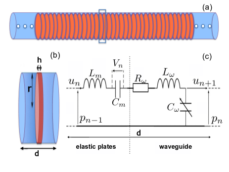
Figure 1: (Color online) (a) Waveguide loaded with an array of elastic plates; (b) the unit-cell of the system; (c) corresponding unit-cell circuit.

Here, we approximate the frequency dependent viscothermal losses by a resistance with a constant value around the frequency of the narrow spectral width envelope solutions that we are interested in.

At this point, we mention that we consider the response of the elastic plate to be linear, while the propagation in the waveguide weakly nonlinear. This is a reasonable approximation, since the pressure amplitudes used in this work are not sufficiently strong to excite nonlinear vibrations of the elastic plateChandrasekharappa and Srirangarajan (1987). On the other hand, it is well known that due to the compressibility of air the wave celerity is nonlinear, $c_{NL}$. This, in turn, lead us to consider that the capacitance $C_{\omega}$ is nonlinear, depending on the pressure $p$, while the inductance is assumed to be linear: $L_{\omega 0}=L_{\omega}$. Approximating the celerity as $c_{NL}\approx c_{0}\left(1+\beta_{0}p/\rho_{0}c_{0}^{2}\right)$, where $\beta_{0}$ is the nonlinear parameter ($\beta_{0}=1.2$ for air), the pressure-dependent capacitance $C_{\omega}$ can be expressed as

$$C_{\omega}\simeq C_{\omega 0}-C_{\omega}^{{}^{\prime}}p_{n},$$ (4)

where $C_{\omega 0}=Sd/\varrho_{0}c_{0}^{2}$ is a constant capacitance (relevant to the linear case) and

$${C_{\omega}^{{}^{\prime}}\simeq\frac{2\beta_{0}}{\rho_{0}c_{0}^{2}}C_{\omega 0}}.$$ (5)

We now apply Kirchhoff’s voltage and current laws in order to derive the discrete nonlinear dissipative evolution equation for the pressure in the $n$-th cell of the lattice:

$$\hat{\delta}^{2}p_{n}=LC_{\omega 0}\frac{d^{2}p_{n}}{dt^{2}}+R_{\omega}C_{\omega 0}\frac{dp_{n}}{dt}+\frac{C_{\omega 0}}{C_{m}}p_{n}-\frac{LC_{\omega}^{{}^{\prime}}}{2}\frac{d^{2}p_{n}^{2}}{dt^{2}}-\frac{R_{\omega}C_{\omega}^{{}^{\prime}}}{2}\frac{dp_{n}^{2}}{dt}-\frac{C_{\omega}^{{}^{\prime}}}{C_{m}}p_{n}^{2},$$ (6)

where $\hat{\delta}^{2}p_{n}\equiv p_{n+1}-2p_{n}+p_{n-1}$, and $L=L_{\omega}+L_{m}$ (see details in Appendix A).

Adopting physically relevant parameter values, we assume that the distance between the plates is $d=0.01$ m and the clamped elastic plates have a thickness $h=2.78\;10^{-4}$ m, radius $r=0.025$ m, as shown in Fig. 1(b), and are made of rubber, with $\rho_{m}=1420$ kg/m³, $E=2.758$ GPa and $\nu=0.34$. Finally, we consider a temperature of $18^{\circ}$ C and the waveguide to be filled by air; thus the specific heat ratio is $\gamma=1.4$, the Prandtl number $Pr=0.71$ and $\eta=1.84\;10^{-5}$ kg/m/s.

II.2 Continuum limit

In order to analytically treat the problem, we focus on the continuum limit of Eq. (6), corresponding to $n\rightarrow\infty$ and $d\rightarrow 0$ (with $nd$ being finite). In such a case, the pressure becomes $p_{n}(t)\rightarrow p(x,t)$, where $x=nd$ is a continuous variable. Then, $p_{n\pm 1}$ can be approximated as:

$${p_{n\pm 1}=p\pm d\frac{\partial p}{\partial x}+\frac{d^{2}}{2}\frac{\partial^{2}p}{\partial x^{2}}\pm\frac{d^{3}}{3!}\frac{\partial^{3}p}{\partial x^{3}}+\frac{d^{4}}{4!}\frac{\partial^{4}p}{\partial x^{4}}+O(d^{5})},$$ (7)

and, accordingly, the operator $\hat{\delta}^{2}p_{n}$ is approximated as: $\hat{\delta}^{2}p_{n}\approx d^{2}p_{xx}+\frac{d^{4}}{12}p_{xxxx}$ (subscripts denote partial derivatives). Here, having kept terms up to order $O(d^{4})$, results in the incorporation of a fourth-order dispersion term in the relevant nonlinear partial differential equation (PDE) –see below. Including such a weak dispersion term, which originates from the periodicity of the elastic plate array (see also Ref. Zhang et al. (2016)), is necessary in order to capture more accurately the dynamics of the system. To this end, neglecting terms of the order $O(d^{5})$ and higher, Eq. (6) is reduced to the following PDE:

$$d^{2}p_{xx}+\frac{d^{4}}{12}p_{xxxx}-LC_{\omega 0}p_{tt}-R_{\omega}C_{\omega 0}p_{t}-\frac{C_{\omega 0}}{C_{m}}p+\frac{1}{2}LC_{\omega}^{{}^{\prime}}\left(p^{2}\right)_{tt}+\frac{1}{2}R_{\omega}C_{\omega}^{{}^{\prime}}\left(p^{2}\right)_{t}+\frac{C_{\omega}^{{}^{\prime}}}{C_{m}}p^{2}=0.$$ (8)

It is also convenient to express our model in dimensionless form; this can be done upon introducing the normalized variables $\tau$ and $\chi$ and the normalized pressure $P$, which are defined as follows: $\tau=\omega_{B}t$ (where $\omega_{B}=\pi c_{0}/d$ is the Bragg frequency), $\chi=(\omega_{B}/c)x$, where the velocity $c$ is given by

$$c=\frac{c_{0}}{\sqrt{1+\alpha}},\quad\alpha=\frac{h\rho_{m}}{d\rho_{0}},$$ (9)

and $p/P_{0}=\epsilon P$, where $P_{0}=\rho_{0}c_{0}^{2}$ and $0<\epsilon\ll 1$ is a formal dimensionless small parameter. Then, Eq. (8) is reduced to the following dimensionless form,

$$P_{\tau\tau}-P_{\chi\chi}-\zeta P_{\chi\chi\chi\chi}+\Gamma P_{\tau}+m^{2}P=\epsilon\beta_{0}\left[2m^{2}P^{2}+\Gamma\left(P^{2}\right)_{\tau}+\left(P^{2}\right)_{\tau\tau}\right],$$ (10)

where parameters $m^{2}$, $\zeta$ and $\Gamma$ are given by

$$m^{2}=\frac{\alpha}{1+\alpha}\left(\frac{\omega_{m}}{\omega_{B}}\right)^{2},\quad\zeta=\frac{1}{12}\pi^{2}(1+\alpha),\quad\Gamma=\frac{R_{\omega}S}{\rho_{0}d\omega_{B}(1+\alpha)}.$$ (11)

It is interesting to identify various limiting cases of Eq. (10). First, in the lossless linear limit $(R_{\omega}=0$, $\Gamma=0$ and $\epsilon\rightarrow 0$), in the long-wavelength approximation (without considering higher-order spatial derivatives, $\zeta\rightarrow 0$), Eq. (10) takes the form of the linear Klein–Gordon (KG) equation Remoissenet (1999); Ablowitz (2011),

$$P_{\tau\tau}-P_{\chi\chi}+m^{2}P=0,$$

with the parameter $m$ playing the role of mass. If the plates are absent ($m^{2}\rightarrow 0$) the Klein–Gordon equation is reduced to the 2nd-order linear wave equation. Another interesting limit of Eq. (10) corresponds to $m^{2}\rightarrow 0$, $\Gamma=0$ and $\zeta\rightarrow 0$, which leads to the well-known Westervelt equation,

$$P_{\tau\tau}-P_{\chi\chi}-\epsilon\beta_{0}\left(P^{2}\right)_{\tau\tau}=0,$$

which is a common nonlinear model describing 1D acoustic wave propagation Hamilton and Blackstock (1998).

II.3 Linear limit

We now consider the linear limit ($\epsilon\rightarrow 0$) of Eq. (10), and assume propagation of plane waves of the form $P\propto\exp[i(k\chi-\omega\tau)]$, to obtain the following dispersion relation

$$D(\omega,k)=(-\omega^{2}+k^{2}-\zeta k^{4}+m^{2})-i\Gamma\omega=0.$$ (12)

Figure 2: (Color online) (a) and (b) respectively show the real and imaginary parts of the complex dispersion relation. Black circles (Red crosses) show the results from the TL (TMM) approach from Eq. (13) (Eq. (14)). Blue dashed (light pink continuous) line shows the lossless dispersion relation obtained from the TL (TMM) approach from the lossless limit of Eq. (13) (Eq. 14). (c) The frequency dependence of $qk^{\prime\prime}$, the product of the dispersion and nonlinearity coefficients of the NLS equation. Light (dark) green region corresponds to the focusing (defocusing) case, with $qk^{\prime\prime}>0$ ($qk^{\prime\prime}<0$).

Equation (12) suggests the existence of a gap at low frequencies, i.e., for $0\leq\omega<m$, with the cut-off frequency defined by the parameter $m$ (as is common in KG–type models Remoissenet (1999); Ablowitz (2011)). For $m<\omega<\omega_{B}$, there exists a propagating band, with the dispersion curve $\omega(k)$ having the form of hyperbola, which asymptotes [according to Eq. (12)] to unity, representing the normalized velocity associated with the linear wave equation $P_{\tau\tau}-P_{\chi\chi}=0$ mentioned above. The term $\zeta k^{4}$ appears to lead to instabilities for large values of $k$. However, both Eqs. (10) and (12) are used in our analysis only in the long-wavelength limit where $k$ is sufficiently small. The term $i\Gamma\omega$ accounts for the viscothermal losses.

Since all quantities in the dispersion relation are dimensionless, it is also relevant to express Eq. (12) in physical units. In particular, taking into account that the frequency $\omega_{ph}$ and wavenumber $k_{ph}$ in physical units are connected with their dimensionless counterparts through $\omega=\omega_{ph}/\omega_{B}$ and $k=\frac{k_{ph}c}{\omega_{B}}$, we can express Eq. (12) in the following form:

$$-\omega_{ph}^{2}+k_{ph}^{2}c^{2}-\zeta\frac{k_{ph}^{4}c^{4}}{\omega_{B}^{2}}+{m}^{2}\omega_{B}^{2}-i\Gamma\omega_{ph}\omega_{B}=0.$$ (13)

The real and imaginary parts of the dispersion relation are respectively plotted in Figs. 2(a) and 2(b). We observe that there is almost no difference between the lossy dispersion relation [Eq. (13)] and the lossless one [Eq. (13) with $\Gamma=0$], since the losses are sufficiently small (see below). The dispersion relation features the band gap from $0$ Hz to $\left(m\frac{\omega_{B}}{2\pi}\right)$ Hz due to the combined effect of the resonance of the plate and of the geometry of the system. The upper limit of the band gap is found to be sufficiently smaller than the Bragg band frequency $f_{B}=c_{0}/2d=17163$ Hz, with $c_{0}=343.26$ m/s. We have compared this analytical dispersion relation with the one obtained via the transfer matrix method (TMM) Bradly (1994). Solid (light pink) lines and (red) crosses in the Figs. 2(a) and 2(b) show the respective results, as obtained using the TMM from the following relation Bradly (1994):

$$\cos(k_{ph}d)=\cos(kd)+i\frac{Z_{m}}{2Z_{c}}\sin(kd),$$ (14)

where $Z_{m}=i\left(\omega_{ph}L_{m}-1/\omega_{ph}C_{m}\right)$ is the impedance of the plate Theocharis et al. (2014), and $Z_{c}$ is given by Eq. (3). For the lossless case [solid (pink) lines in Figs. 2(a) and 2(b)], the wavenumber and the acoustic characteristic impedance of the waveguide reduce to $k=\omega_{ph}/c_{0}$ and $Z_{c}=\rho_{0}c_{0}/S$ respectively. Comparing the dispersion relation obtained by using TMM, with the one resulting from the continuum approximation, we find an excellent agreement between these two in the regime of low frequencies.

III Envelope solitons

In this Section, we apply the multiple scales perturbation method to reduce Eq. (10) to an effective NLS equation. This way, we derive approximate analytical envelope soliton solutions of the original lattice system, and study their dynamics –by means of direct numerical simulations and soliton perturbation theory– in the absence and presence of viscothermal losses.

III.1 Bright solitons: propagating solitary waves

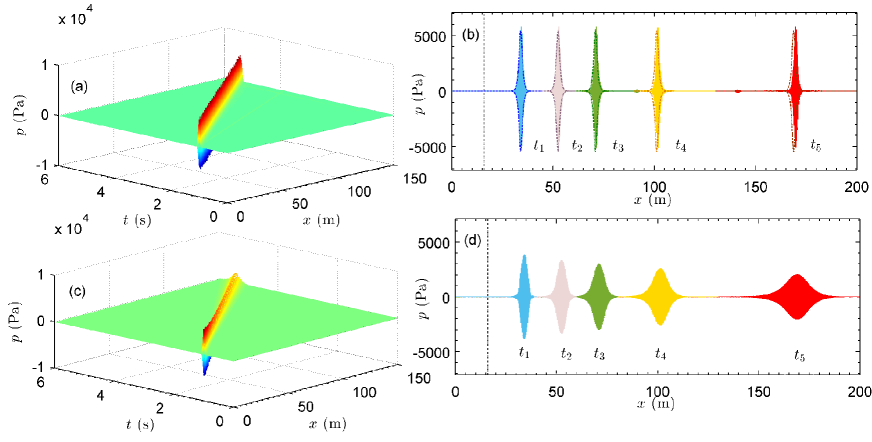
Figure 3: (Color online) (a) 3D plot depicting the evolution of a bright soliton of the form of Eq. (27), obtained by numerically integrating the lossless version of Eq. (6) ($R_{\omega}=0$) with $\epsilon=0.018$ ($2\epsilon\eta P_{0}=5471$ Pa), $f=369$ Hz. (b) Numerical spatial profiles of the bright soliton measured at $t_{1}=2$ s (light blue line), $t_{2}=2.5$ s (light pink line), $t_{3}=3$ s (light green line), $t_{4}=4$ s (light yellow line), and $t_{5}=5.7$ s (red line). Blue dashed line, pink dashed line, green dashed line, yellow dashed line, and dark red dashed line stand for the analytical envelope results of Eq. (27) at $t_{1}$, $t_{2}$, $t_{3}$, $t_{4}$ and $t_{5}$ respectively. Black dash-dotted line stand for the nonlinear length $L_{NL}$ and the dispersion length $L_{D}$, where $L_{NL}=L_{D}=16$ m; (c) Turn off the nonlinearity effect, 3D plot depicting the dispersive effect numerically obtained. (d) Numerical spatial profile of dispersive effect measured at $t_{1}$ (light blue line), $t_{2}$ (light pink line), $t_{3}$ (light green line), $t_{4}$ (light yellow line), and $t_{5}$ (red line).

We start our analysis by introducing the slow variables,

$$\chi_{n}=\epsilon^{n}\chi,\quad\tau_{n}=\epsilon^{n}\tau,\quad n=0,1,2,\ldots,$$ (15)

and express $P$ as an asymptotic series in $\epsilon$, namely:

$$P=p_{0}+\epsilon p_{1}+\epsilon^{2}p_{2}+\ldots.$$ (16)

Then, substituting the above into Eq. (10) we obtain a hierarchy of equations at various orders in $\epsilon$ (see Appendix B). This way, and assuming that the losses are sufficiently small, namely $\Gamma\rightarrow\epsilon^{2}\Gamma$, we obtain the following results.

First, at the leading order, i.e. at $O(\epsilon^{0})$, we find that $p_{0}$ satisfies a linear wave equation [cf. Eq. (B1) in Appendix B], and thus is of the form:

$$p_{0}=A(\chi_{1},\chi_{2},\cdots,\tau_{1},\tau_{2},\cdots)\exp(i\theta)+{\rm c.c.},$$ (17)

where $A$ is an unknown envelope function, $\theta=k\chi_{0}-\omega\tau_{0}$, with the wavenumber $k$ and frequency $\omega$ satisfying the dispersion relation (12) (c.c. denotes complex conjugate).

Next, at the order $O(\epsilon^{1})$, we obtain an equation whose solvability condition requires that the secular part [i.e., the term $\propto\exp(i\theta)$] vanishes. This yields the following equation,

$$\left(k^{\prime}\frac{\partial}{\partial\tau_{1}}+\frac{\partial}{\partial\chi_{1}}\right)A(\chi_{1},\chi_{2},\cdots,\tau_{1},\tau_{2},\cdots)=0,$$ (18)

where the inverse group velocity $k^{\prime}\equiv\partial k/\partial\omega=1/v_{g}$ is given by

$$k^{\prime}=\frac{\omega}{k-2\zeta k^{3}}.$$ (19)

Equation (18) is satisfied as long as $A$ depends on the variables $\chi_{1}$ and $\tau_{1}$ through the traveling-wave coordinate $\tilde{\tau}_{1}=\tau_{1}-k^{\prime}\chi_{1}$ (i.e., $A$ travels with the group velocity), namely $A(\chi_{1},\tau_{1},\chi_{2},\tau_{2},\cdots)=A(\tilde{\tau}_{1},\chi_{2},\tau_{2},\cdots)$. Additionally, at the same order, we obtain the form of the field $p_{1}$, namely,

$$p_{1}=2\beta_{0}\frac{m^{2}-2\omega^{2}}{D(2\omega,2k)}A^{2}e^{2i\theta}+Be^{i\theta}+4\beta_{0}\left|A\right|^{2}+{\rm c.c.},$$ (20)

where $B$ is an unknown function that can be found at a higher-order approximation.

Finally, employing the non-secularity condition at $O(\epsilon^{2})$, yields the following PDE for the envelope function $A$,

$$i\frac{\partial A}{\partial\chi_{2}}-\frac{1}{2}k^{\prime\prime}\frac{\partial^{2}A}{\partial\tilde{\tau}_{1}^{2}}-q\left|A\right|^{2}A=-i\Lambda A,$$ (21)

which is a NLS equation incorporating a linear loss term. The dispersion, nonlinearity and dissipation coefficients are respectively given by:

$$k^{\prime\prime}\equiv\frac{\partial^{2}k}{\partial\omega^{2}}=\frac{1-k^{\prime 2}+6\zeta k^{2}k^{\prime 2}}{k-2\zeta k^{3}},$$ (22)

$$q(\omega,k)=\beta_{0}^{2}\frac{2(2m^{2}-\omega^{2})(m^{2}-2\omega^{2})}{3(m^{2}+4\zeta k^{4})(k-2\zeta k^{3})}-\beta_{0}^{2}\frac{4(2m^{2}-\omega^{2})}{(k-2\zeta k^{3})},$$ (23)

$$\Lambda=\frac{\omega\Gamma}{2(k_{r}-2\zeta k_{r}^{3})}.$$ (24)

The sign of the product $\sigma\equiv{\rm sgn}(qk^{\prime\prime})$ determines the nature of the NLS equation and its solutions Remoissenet (1999); Ablowitz (2011). In particular, in the case $\sigma=+1$ ($\sigma=-1$) the NLS is called focusing (defocusing) and supports bright (dark) soliton solutions. Bright solitons are localized waves with vanishing tails towards infinity, while dark solitons are density dips, with a phase jump across the density minimum, on top of a non-vaninishing continuous wave background. Figure 2(c) shows the frequency dependence of the product $qk^{{}^{\prime\prime}}$ for the system. We observe three different regimes: focusing regime ($\sigma=+1$) at low frequencies (light green region), defocusing regime ($\sigma=-1$) at intermediate frequencies (dark green region), and another focusing regime ($\sigma=+1$) at high frequencies (light green region). Below we focus on the case of the focusing NLS equation and study propagating bright solitons and stationary gap solitons that are supported in this case.

The dispersion length, $L_{D}$, and the nonlinearity length, $L_{NL}$, provide the length scales over which dispersive or nonlinear effects become important for pulse evolution. For solitons, where the nonlinearity and dispersion effects should be perfectly balanced, $L_{D}\simeq L_{NL}$ (see Appendix C for details). For frequencies larger than $435$ Hz, the dispersion is very weak leading (e.g., for $\epsilon=0.018$ and $f=435$ Hz) to a dispersion length of the order of $L_{D}=450$ m. Here, we focus on the low frequency region (light green region from $305.7$ Hz to $432.3$ Hz) described by an effective focusing NLS with linear loss, in order to study the combined effect of (a relatively strong) dispersion and nonlinearity.

III.1.1 Bright solitons in the absence of losses

In the absence of losses ($\Gamma=0$), the analytical bright soliton solution for the envelope function $A$ is of the form,

$$A=\eta\textrm{sech}\left(\eta\sqrt{\left|\frac{q}{k^{{}^{\prime\prime}}}\right|}\tilde{\tau}_{1}\right)\exp\left(-i\frac{q\eta^{2}}{2}\chi_{2}\right),$$ (25)

where $\eta$ is a free parameter setting the soliton amplitude. The corresponding approximate solution of Eq. (10) is expressed, as a function of parameters $\chi$ and $\tau$, as follows:

$$P(\chi,\tau)\approx 2\eta\textrm{sech}\left[\epsilon\eta\sqrt{\left|\frac{q}{k^{\prime\prime}}\right|}\left(\tau-k^{\prime}\chi\right)\right]\cos\left(\omega\tau-k\chi-\frac{q\epsilon^{2}\eta^{2}}{2}\chi\right).$$ (26)

Futhermore, in the original space and time coordinates, $x$ and $t$, the approximate envelope soliton solution for the pressure $p$ reads:

$$\frac{p(x,t)}{P_{0}}\approx 2\epsilon\eta\textrm{sech}\left[\epsilon\eta\sqrt{\left|\frac{q}{k^{\prime\prime}}\right|}\omega_{B}\left(t-\frac{k^{\prime}\sqrt{1+\alpha}}{c_{0}}x\right)\right]\cos\left(\omega\omega_{B}t-k\omega_{B}\frac{\sqrt{1+\alpha}}{c_{0}}x-\frac{q\epsilon^{2}\eta^{2}}{2}\omega_{B}\frac{\sqrt{1+\alpha}}{c_{0}}x\right).$$ (27)

This bright soliton is characterized by an amplitude $2\epsilon\eta P_{0}$ and a width $(\epsilon\eta\sqrt{|\frac{q}{k^{\prime\prime}}|})^{-1}$. In addition, its velocity is given by the group velocity $c_{0}/(k^{\prime}\sqrt{1+\alpha})$ at the carrier frequency and in contrast with soliton solutions of other nonlinear dispersive wave equation other soliton solutions, like for instance the soliton of e.g., the Korteweg-de Vries (KdV) equation Ablowitz (2011) is independent of its amplitude.

Figure 4: (Color online)(a) Spectra of the different drivers, of the form of Eq. (27), introduced at $x=0$: $\epsilon=0.008$ ($2\epsilon\eta P_{0}=2431$ Pa) at $369$ Hz (red dashed line); $\epsilon=0.018$ ($2\epsilon\eta P_{0}=5471$ Pa) at $369$ Hz (thick light blue continuous line) and $\epsilon=0.018$ at $307.3$ Hz (thin black continuous line). (b) Space-time diagrams of the different wave packet generated from the different drivers in (a). Symbols stand for the analytical space-time diagrams at $369$ Hz and $307.3$ Hz. The slopes of the lines depict the corresponding group velocities. (c) Numerical time evolutions of the maximum pressure value of the solitons for the different drivers.

Let us now proceed by studying numerically the evolution of the approximate soliton solution of Eq. (27), in the framework of the fully discrete model of Eq. (6). We start with the lossless case ($R_{\omega}=0$) and a driver of the form given by Eq. (27) at $x=0$. We use the parameter values $\epsilon=0.018$ ($2\epsilon\eta P_{0}=5471$ Pa) and $f=369$ Hz. The results of the simulations are shown in Figs. 3(a) and 3(b). We observe that the input envelope wave propagates with a constant amplitude and width as shown in the spatio-temporal evolution in Fig. 3(a). The direct comparison of analytics and simulations is shown in Fig. 3(b). Here, the envelope soliton solution of Eq. (27), is compared at five different instants with the numerical results for the discrete wave equation showing a very good agreement. Thus, we confirm that the NLS approximation is able to capture the propagation of envelope solitons of the discrete model (6). To emphasize the effect of the counterbalance of dispersion by nonlinearity, we also show the evolution of the same envelope function when the nonlinearity is turned off. As shown in Figs. 3(c) and 3(d), the initial wavepacket spreads as it propagates due to dispersion.

Next, we study the validity of the multiple-scales perturbation theory and the properties of the corresponding bright solitons. To do so, we study three different solutions: two at the same carrier frequency $f=369$ Hz with different amplitudes, $\epsilon=0.008$ ($2\epsilon\eta P_{0}=2431$ Pa), and $\epsilon=0.018$ ($2\epsilon\eta P_{0}=5471$ Pa) and one of amplitude $\epsilon=0.018$ ($2\epsilon\eta P_{0}=5471$ Pa) and carrier frequency $f=307.3$ Hz. The respective spectra of these solitons are depicted in Fig. 4(a). Note that, for the last case, part of the spectrum of the soliton lies inside the gap. Starting with the two soliton solutions at the same carrier frequency but different amplitudes, we expect them to propagate with the same velocity, i.e., the group velocity. In Fig. 4(b), the dashed red and solid cyan lines show the the position of the maximum of the numerical solution as a function of time, for $\epsilon=0.008$ and $\epsilon=0.018$, respectively. Green crosses depicts the analytical group velocity. Both solutions appear to follow with a very good agreement with the analytical prediction. In addition, as shown in Fig. 4(c), these solutions propagate with constant amplitude. However, as seen in the inset of Fig. 4(b), there is a small discrepancy in the velocity of the envelope solutions of larger amplitude. This indicates a deviation from the effective NLS description for large amplitudes, which is naturally expected due to the perturbative nature of our analytical approach. Note, that this small deviation is also depicted in Fig. 3(b) for the last time instant.

The third case corresponds to the solution whose part of its spectrum lies in the gap, for $\epsilon=0.018$ and $f=307.3$ Hz. Here, we observe the propagation of a breathing solitary solution. The respective long-lived, weakly damped periodic oscillations of the soliton amplitude are depicted in Fig. 4(c). As it has been discussed Pelinovsky et al. (1998); Kivshar et al. (1998), this behavior may be associated to the birth of an internal mode of the soliton. We also observe a small deviation between the numerical group velocity and the corresponding analytical one, as shown in Fig. 4(b).

III.1.2 Bright solitary waves in the presence of losses

Figure 5: (Color online) Effect of viscothermal losses on traveling bright solitons. Evolution of the maximum pressure in time for the lossy bright soliton (continuous red line for numerical results and blue crosses for the analytical ones) and for linear lossy dispersive wave (dashed yellow line for numerical results). The driver corresponds to $\epsilon=0.018$ ($2\epsilon\eta P_{0}=5471$ Pa) and $f=369$ Hz. (a) Propagation in a weakly lossy medium where $R_{\omega}=6.8$ Ohm; (b) Propagation in a real lossy medium where $R_{\omega}=68.04$ Ohm.

Having established the validity of the NLS solitons in the lossless version of the discrete model (6), we proceed by studying the evolution of the envelope solitons under the presence of the viscothermal losses. We numerically integrate the nonlinear lattice model with $R_{\omega}=6.8$ Ohm and with $R_{\omega}=68.04$ Ohm, using a driver corresponding to the soliton shown in Fig. 4 with parameters $\epsilon=0.018$, and $f=369$ Hz.

As shown in Fig. 5(a), for the small resistor of $R_{\omega}=6.8$ Ohm, the amplitude of the soliton is found to be weakly attenuated. In contrast, in the linear dispersive case (see dashed orange line) the combined effect of dispersion and losses strongly attenuates the wave packet. Let us next consider the case of the large resistance, $R_{\omega}=68.4$ Ohm, corresponding to the viscothermal losses at $f=369$ Hz, assuming an air-filled waveguide at $18^{\circ}$ C. In this case, as shown in Fig. 5(b) the effect of losses on the soliton amplitude is (naturally) more pronounced, but still less than the case without considering the nonlinearity [dashed yellow line in Fig. 5(b)]. Here, we also mention that the above findings are valid for the particular (physically relevant) scenarios discussed above. Indeed, generally, since –as discussed above– dispersion, nonlinearity and dissipation set pertinent scales, it is exactly this scale competition that defines the nature of the dynamics.

Losses have been considered weak in the multiple-scale perturbation method, leading to the effective NLS (21) with the linear loss. Furthermore, as long as the parameter $\Lambda$ is small enough, it is possible to analytically study the role of such a dissipation on the soliton dynamics. Indeed, according to soliton perturbation theory (see, e.g., Ref. [Agrawal., 1989]), the linear loss does not affect the velocity of the soliton but its amplitude $\eta$ becomes a decaying function of time. The evolution of $\eta$, can be determined by the evolution of the norm, and it is straightforward to find that it is described as follows:

$$\eta(\chi_{2})=\eta(0)\exp(-2\Lambda\chi_{2}).$$ (28)

Thus, in terms of the original coordinates, the amplitude of the bright soliton decreases exponentially according to:

$$\eta(x)=\eta(0)\exp\left(-2\Lambda\epsilon^{2}\omega_{B}\frac{\sqrt{1+\alpha}}{c_{0}}x\right).$$ (29)

This analytical result is denoted in Fig. 5 by crosses. For the case of $R=6.8$ Ohm –Fig. 5(a)– the agreement between numerical simulations and soliton perturbation theory is excellent. For the case of $R=68.04$ Ohm –Fig. 5(b)– the analytical result describes fairly well the amplitude attenuation observed in simulations. For both cases, we also confirm in the simulations that the envelope solutions propagate with a constant velocity equal to $v_{g}$. We can thus conclude that even in the presence of realistic viscothermal losses, the system supports envelope solitary waves that are described, in a very good approximation, by the effective NLS (21) with the linear loss.

III.2 Gap solitons: stationary solitary waves

While in Sec. III.1 we introduced the traveling bright soliton propagating with group velocity $v_{g}$, now we will study stationary (i.e., non-traveling) localized waveforms oscillating at a frequency in the band gap of the system; these structures are called gap solitons.

In order to identify such solitons, which evolve in time rather than space, we need to derive a variant of the NLS model with the evolution variable being the time. To do so, returning back to our perturbation scheme, in the solvability condition of the equation at the order $O(\epsilon^{1})$, we use the variable $\xi_{1}=\chi_{1}-v_{g}\tau_{1}$. This way, we obtain:

$$\left(\frac{\partial}{\partial\tau_{1}}+v_{g}\frac{\partial}{\partial\chi_{1}}\right)A(\chi_{1},\chi_{2},\cdots,\tau_{1},\tau_{2},\cdots)=0,$$ (30)

which is satisfied as long as $A$ depends on the variables $\chi_{1}$ and $\tau_{1}$ through the traveling-wave coordinate $\tilde{\xi}_{1}$, namely $A(\chi_{1},\tau_{1},\chi_{2},\tau_{2},\cdots)=A(\xi_{1},\chi_{2},\tau_{2},\cdots)$ [in this case, $p_{1}$ is again given by Eq. (20)]. Then, the non-secularity condition at $O(\epsilon^{2})$ leads to the following NLS equation,

$$i\frac{\partial A}{\partial T_{2}}-\frac{1}{2}v_{g}^{3}k^{{}^{\prime\prime}}\frac{\partial^{2}A}{\partial\tilde{\xi}_{1}^{2}}-v_{g}q\left|A\right|^{2}A=-iv_{g}\Lambda A,$$ (31)

which is directly connected to Eq. (21) by a change of the coordinate system.

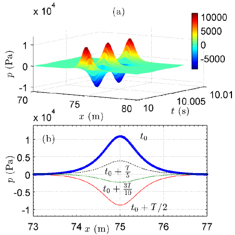
Figure 6: (Color online) (a) 3D plot depicting the evolution of a gap soliton of the form of Eq. (35), obtained by numerically integrating the lossless version of Eq. (6) ($R_{\omega}=0$) with $\epsilon=0.04$ ($2\epsilon\eta P_{0}=12158$ Pa), in a lattice with a length of $150$ m. (b) Numerical spatial profiles of gap soliton measured from $t_{0}$ (at which gap soliton has a maximal amplitude) to $t_{0}+T/2$ (at which gap soliton has a minimal amplitude).

Figure 7: (Color online) (a) Amplitude dependence of the frequency of the gap soliton. Blue line stands for the analytical results, Eq. (34). Red circles stand for the numerical results, where the numerical values of the amplitudes and the frequencies are getting from the main peak of the spectrum of the different gap solitons obtained by numerically integrating the lossless version of Eq. (6) ($R_{\omega}=0$) with different initial amplitudes. Black dashed line stands for the cut-off frequency of the system. (b) Time evolution of the middle point of the gap soliton in Fig. 6.

Figure 8: (Color online) Numerical study of the effect of viscothermal losses on gap solitons. The Eq. (35) with $\epsilon=0.04$ ($2\epsilon\eta P_{0}=12158$ Pa) is the initial condition for the gap soliton. (a) and (c) represents the time evolution of the middle point of the gap soliton propagating in a weakly lossy medium where $R_{\omega}=6.18$ Ohm and $R_{\omega}=61.8$ Ohm respectively (Blue lines for numerical results and red crosses stand for the analytical time evolution of the maximum pressure for the lossy gap solitons). (b) and (d) show the spectra of the gap soliton propagating in a lossy medium. Continuous line is the fast Fourier transform (FFT) of the first part of the signal in Fig. 8(a) and Fig. 8(c) and dashed line is the FFT of the last part of the signal in Fig. 8(a) and Fig. 8(c) respectively.

III.2.1 Gap solitons in the absence of losses

In the absence of losses ($\Lambda=0$), the analytical soliton solution for the envelope is of the form,

$$A=\eta\textrm{sech}\left[\epsilon\eta\sqrt{\left|\frac{q}{k"}\right|}\frac{1}{v_{g}}(\chi-v_{g}\tau)\right]\exp(-i\epsilon^{2}\eta^{2}\frac{qv_{g}}{2}\tau),$$ (32)

where, as before, $\eta$ sets the amplitude of the soliton.

Considering the case with $\omega=m$ and $k=0$, gap soliton solutions of Eq. (10) can then be written in terms of coordinates $\chi$ and $\tau$ as

$$P(\chi,\tau)\approx 2\eta\textrm{sech}\left(\epsilon\eta\sqrt{\frac{14}{3}}m\beta_{0}\chi\right)\cos\left(\Omega_{m}\tau\right),$$ (33)

where

$$\Omega_{m}=m-\frac{7}{3}\epsilon^{2}\eta^{2}m\beta_{0}^{2}.$$ (34)

In terms of the original space and time coordinates, the approximate envelope gap soliton solution for the pressure $p$ centred at position $x_{0}$ is the following,

$$p(x,t) = 2\epsilon\eta P_{0}\textrm{sech}\left[\epsilon\eta\sqrt{\frac{14}{3}}m\beta_{0}\omega_{B}\frac{\sqrt{1+\alpha}}{c_{0}}(x-x_{0})\right]$$ (35)

$$\times \cos\left(\Omega_{m}\omega_{B}t\right).$$

The gap soliton, which is a solution that does not move, is characterized by an amplitude $2\epsilon\eta P_{0}$. Its width also depends on amplitude and it oscillates in time with a period $T=2\pi/\Omega_{m}\omega_{B}$.

To study these solutions, we numerically integrate the nonlinear lossless lattice model, Eq. (6) with $R_{\omega}=0$, using an initial condition given by Eq. (35) for $t=0$ and $x_{0}=75$ m. An example of a gap soliton with $\epsilon=0.04$ ($2\epsilon\eta P_{0}=12158$ Pa) is shown in Fig. 6. Figure 6(a) shows the spatio-temporal evolution of the gap soliton during a time interval of three periods. Figure 6(b) depicts the numerical spatial profiles of the gap soliton measured from $t_{0}$ (at which gap soliton has a maximal amplitude) to $t_{0}+T/2$. Note that, the absolute value of the maximal amplitude is bigger than that of the minimal amplitude of the gap soliton. This asymmetry is caused by the term $\propto|A|^{2}$ in Eq. (20).

We have calculated both numerically and analytically the frequency of the gap soliton for different amplitudes, as shown in Fig. 7(a). As expected by Eq. (34), the frequency of the gap soliton lies in the band gap (blue continuous line); red crosses depict the numerical results. Each point, represents the frequency of the main peak of the spectrum after numerical integration of the lossless version of Eq. (6) ($R_{\omega}=0$). It is clearly observed that the analytical results are in a good agreement with the numerical ones.

The long time evolution of the center of the gap soliton solution is shown in Fig. 7(b). First we note that the amplitude exhibits a long-lived oscillation. This can be associated, as in the previous case of the bright solitons, to the birth of an internal modePelinovsky et al. (1998); Kivshar et al. (1998). These beatings are diminished with time as the initial approximate solution radiates and approaches the numerically exact gap soliton solution of the lattice nonlinear equation.

III.2.2 Gap solitons in the presence of losses

We next study numerically the effect of viscothermal losses on the gap soliton. We numerically integrate Eq. (6) considering the weak and strong lossy cases, as for the bright soliton. The initial condition is of the form of Eq. (35) with $t=0$ and $x_{0}=75$ m. We use an amplitude of $\epsilon=0.04$ ($2\epsilon\eta P_{0}=12158$ Pa) and carrier frequency $f=304$ Hz. Figures 8(a) and 8(b) correspond to the temporal evolution and evolution of the frequency spectrum of the amplitude of the gap soliton at $x_{0}$ in a weakly lossy medium, respectively. We observe that the amplitude of the gap soliton decreases slowly with time. As a result, the frequency increases, moving towards the cut-off frequency, see Fig. 8(b). This is predicted from Eq. (34) and illustrated in Fig. 7(a).

Analogously, we can see in Figs. 8(c) and 8(d) the temporal evolution and frequency spectrum of the amplitude of the gap soliton at $x_{0}$ in a strong lossy medium respectively. In this case, we observe that the amplitude of the gap soliton decays faster than in the weakly lossy medium, –see Fig. 8(c)– and finally its frequency approaches to the cut off frequency.

Analytical solutions of the lossy problem can also be obtained for the gap solitons. In particular, following soliton perturbation theory as before, the evolution of the amplitude of the gap soliton $\eta$ is found to be:

$$\eta(T_{2})=\eta(0)\exp(-2v_{g}\Lambda T_{2}).$$ (36)

In terms of the original time coordinate, the amplitude of the gap soliton decreases exponentially as

$$\eta(t)=\eta(0)\exp(-2v_{g}\Lambda\epsilon^{2}\omega_{B}t).$$ (37)

The analytical results are shown in Figs. 8(a) and 8(c), and are found in a good agreement with the numerical results.

IV Conclusions

In conclusion, we have theoretically and numerically studied envelope solitonic structures, namely bright and gap solitons, in a 1D acoustic metamaterial composed of an air-filled tube with a periodic array of clamped elastic plates. Based on the electro-acoustic analogy, we utilized the transmission line (TL) approach to derive a lossy nonlinear lattice model. Considering the continuum limit of the latter, we derived a nonlinear dispersive and dissipative wave equation. In the linear limit, the dispersion relation was found to be in good agreement with the one obtained by the transfer matrix method. No essential difference between the lossy dispersion relation and the lossless one was found, because losses are sufficiently small, i.e., the lossy term can be treated as a small perturbation.

We have thus used a multiple scale perturbative approach to derive an effective NLS model, and analytically predict the existence of both bright and gap solitons. The dynamics of these structures were studied in the absence and in the presence of viscothermal losses. Analytical and numerical results were found to be in very good agreement. It is thus concluded that 1D acoustic membrane-type metamaterial can support envelope solitary waves even in the presence of realistic viscothermal losses. Our results pave the way for the study of nonlinear coherent structures in higher-dimensional settings, as well as in double negative metamaterials.

Appendix A Electro-Acoustic Analogue Modeling

Here, we derive the evolution equation (considering lossy effect of the waveguide) for the pressure in the $n$-th cell of the lattice, as follows.

First, we note that the advantage of the considered unit-cell circuit is that the inductances $L_{\omega}$ and $L_{m}$ are in a series connection and, thus, can be substituted by the global inductance $L=L_{\omega}+L_{m}$ (see Fig. 1(c)).

Applying Kirchoff’s voltage law for two successive cells yields

$$p_{n-1}-p_{n}=L\frac{d}{dt}u_{n}+V_{n}+R_{\omega}u_{n},$$ (38)

$$p_{n}-p_{n+1}=L\frac{d}{dt}u_{n+1}+V_{n+1}+R_{\omega}u_{n+1},$$ (39)

where $V_{n}$ is the voltage produced by the capacitance of the elastic plates $C_{m}$. Subtracting the two equations above, we obtain the differential-difference equation (DDE)

$$\hat{\delta}^{2}p_{n}=L\frac{d}{dt}\left(u_{n}-u_{n+1}\right)+R_{\omega}\left(u_{n}-u_{n+1}\right)+\left(V_{n}-V_{n+1}\right),$$ (40)

where $\hat{\delta}^{2}p_{n}\equiv p_{n+1}-2p_{n}+p_{n-1}$. Then, Kirchhoff’s current law yields

$$u_{n}-u_{n+1}=C_{\omega}\frac{d}{dt}\left(p_{n}\right),$$ (41)

with

$$u_{n}=C_{m}\frac{d}{dt}\left(V_{n}\right)\quad\mbox{and}\quad u_{n+1}=C_{m}\frac{d}{dt}\left(V_{n+1}\right).$$ (42)

Subtracting Eq. (42) and employing Eq. (41), we obtain

$$u_{n}-u_{n+1}=C_{m}\frac{d}{dt}\left(V_{n}-V_{n+1}\right)=C_{\omega}\frac{d}{dt}\left(p_{n}\right).$$ (43)

Then, recalling that the capacitance $C_{\omega}$ depends on the pressure (cf. Eq. (4)), we express $V_{n}-V_{n+1}$ as

$$V_{n}-V_{n+1}=\frac{C_{\omega}}{C_{m}}p_{n}=\frac{C_{\omega 0}}{C_{m}}p_{n}-\frac{C_{\omega}^{{}^{\prime}}}{C_{m}}p_{n}^{2}.$$ (44)

Next, substituting Eq. (43) and Eq. (44) into Eq. (40), we obtain the following evolution equation for the pressure

$$\hat{\delta}^{2}p_{n}=L\frac{d}{dt}\left(C_{\omega}\frac{d}{dt}\left(p_{n}\right)\right)+R_{\omega}\left(C_{\omega}\frac{d}{dt}\left(p_{n}\right)\right)+\frac{C_{\omega}}{C_{m}}p_{n}.$$ (45)

To this end, employing Eq. (4), we can rewrite the above equation, then we get the evolution equation (considering lossy effect of the waveguide) for the pressure in the $n$-th cell of the lattice, Eq. (6).

Appendix B Hierarchy of equations in multiple scale perturbation method

There we present the hierarchy of equations at various orders in $\epsilon$,

$$O(\epsilon^{0}):\widehat{L}_{0}p_{0}=0,$$ (46)

$$O(\epsilon^{1}):\widehat{L}_{0}p_{1}+\widehat{L}_{1}p_{0}=\widehat{N}_{0}\left[p_{0}^{2}\right],$$ (47)

$$O(\epsilon^{2}):\widehat{L}_{0}p_{2}+\widehat{L}_{1}p_{1}+\widehat{L}_{2}p_{0}=\widehat{N}_{0}\left[2p_{0}p_{1}\right]+\widehat{N}_{1}\left[p_{0}^{2}\right],$$ (48)

where linear operators $\widehat{L}_{0}$, $\widehat{L}_{1}$ and $\widehat{L}_{2}$, as well as the nonlinear operators $\widehat{N}_{0}$, $\widehat{N}_{1}$ are given by

$$\widehat{L}_{0}=-\frac{\partial^{2}}{\partial\chi_{0}^{2}}+\frac{\partial^{2}}{\partial\tau_{0}^{2}}-\zeta\frac{\partial^{4}}{\partial\chi_{0}^{4}}+m^{2},$$ (49)

$$\widehat{L}_{1}=-2\frac{\partial^{2}}{\partial\chi_{0}\chi_{1}}+2\frac{\partial^{2}}{\partial\tau_{0}\tau_{1}}-4\zeta\frac{\partial^{4}}{\partial\chi_{0}^{3}\partial\chi_{1}},$$ (50)

$$\widehat{L}_{2}= -\frac{\partial^{2}}{\partial\chi_{1}^{2}}-2\frac{\partial^{2}}{\partial\chi_{0}\chi_{2}}+\frac{\partial^{2}}{\partial\tau_{1}^{2}}+2\frac{\partial^{2}}{\partial\tau_{0}\tau_{2}}$$ (51)

$$-\zeta\left(6\frac{\partial^{4}}{\partial\chi_{0}^{2}\partial\chi_{1}^{2}}+4\frac{\partial^{4}}{\partial\chi_{0}^{3}\partial\chi_{2}}\right)+\Gamma\frac{\partial}{\partial\tau_{0}},$$

$$\widehat{N}_{0}=\beta_{0}\frac{\partial^{2}}{\partial\tau_{0}^{2}}+2\beta_{0}m^{2},$$ (52)

$$\widehat{N}_{1}=2\beta_{0}\frac{\partial^{2}}{\partial\tau_{0}\tau_{1}}.$$ (53)

Appendix C Nonlinear length and dispersion length

Here is the calculation for nonlinear length and dispersion length.

We can rewrite Eq. (21) in its dimensional form as

$$i\frac{\partial\phi}{\partial x}-\frac{1}{2}k_{ph}^{{}^{\prime\prime}}\frac{\partial^{2}\phi}{\partial T^{2}}-q_{ph}\left|\phi\right|^{2}\phi=0,$$ (54)

where

$$k_{ph}^{{}^{\prime\prime}}=\frac{k^{\prime\prime}}{\omega_{B}c},\quad q_{ph}=q(\omega,k)\frac{\omega_{B}}{c}\frac{1}{P_{0}^{2}},$$ (55)

and $\phi/P_{0}=\epsilon A$, $T=t-x/v_{g}$, $v_{g}=\partial\omega_{ph}/\partial k_{ph}$.

In order to get the dispersion length and the nonlinearity length, we introduce $t_{0}$ and $A_{0}$ as the characteristic width of the initial condition, and the maximum pressure of the initial condition respectivelly. Then we use the new time variable $\tilde{T}=T/t_{0}$ and substitute $\phi=A_{0}\Phi$ to obtain

$$i\frac{\partial\Phi}{\partial x}-\frac{1}{2L_{D}}\frac{\partial^{2}\Phi}{\partial\tilde{T}^{2}}-\frac{1}{L_{NL}}\left|\Phi\right|^{2}\Phi=0,$$ (56)

where the characteristic lengths are defined as,

$$L_{D}=\frac{t_{0}^{2}}{\left|k_{ph}^{{}^{\prime\prime}}\right|},\mbox{ and}L_{NL}=\frac{1}{\left|q_{ph}\right|A_{0}^{2}}.$$ (57)

According to Eq. (25), here we define,

$$t_{0}=\left(\epsilon\eta\sqrt{\left|\frac{q}{k^{{}^{\prime\prime}}}\right|}\omega_{B}\right)^{-1},\quad\mbox{ and }A_{0}=\epsilon\eta P_{0}.$$ (58)

Thus $L_{NL}/L_{D}\sim 1$.

References

- Sugimoto and Horioka (1995) N. Sugimoto and T. Horioka, J. Acoust. Soc. Am. 97 (1995).
- Bradly (1994) C. E. Bradly, J. Acoust. Soc. Am. 96 (1994).
- Liu et al. (2000) Z. Liu, X. Zhang, Y. Mao, Y. Y. Zhu, Z. Yang, C. T. Chan, and P. Sheng, Science 289 (2000).
- Sukhovich et al. (2009) A. Sukhovich, B. Merheb, K. Muralidharan, J. O. Vasseur, Y. Pennec, P. A. Deymier, and J. H. Page, Phys. Rev. Lett. 102 (2009).
- Sanchis et al. (2013) L. Sanchis, V. M. García-Chocano, R. Llopis-Pontiveros, A. Climente, J. Martínez-Pastor, F. Cervera, and J. Sánchez-Dehesa., Phys. Rev. Lett. 110 (2013).
- Ma et al. (2014) G. Ma, M. Yang, S. Xiao, Z. Yang, and P. Sheng, Nature Mater. 13 (2014).
- Romero-García et al. (2016) V. Romero-García, G. Theocharis, O. Richoux, A. Merkel, V. Tournat, and V. Pagneux, Sci. Rep. 6 (2016).
- Park et al. (2013) J. J. Park, K. J. B. Lee, O. B. Wright, M. K. Jung, and S. H. Lee., Phys. Rev. Lett. 110 (2013).
- Deymier (2013) P. A. Deymier, Acoustic Metamaterials and Phononic Crystals (Springer Series, 2013).
- Naugolnykh and Ostrovsky (1998) K. Naugolnykh and L. Ostrovsky, Nonlinear Wave Processes in Acoustics (Cambridge Texts in Applied Mathematics, 1998).
- Bradley (1995) C. E. Bradley, J. Acoust. Soc. Am. 98(5) (1995).
- Sugimoto et al. (1999) N. Sugimoto, M. Masuda, J. Ohno, and D. Motoi, Phys. Rev. Lett. 83 (1999).
- Sugimoto et al. (2003) N. Sugimoto, M. Masuda, and T. Hashiguchi, J. Acoust. Soc. Am. 114(4) (2003).
- Richoux et al. (2015) O. Richoux, B. Lombard, and J.-F. Mercier., Wave Motion 56, 85 (2015).
- Zwikker and Kosten (1949) C. Zwikker and C. W. Kosten, Sound absorbing materials (Elsevier, 1949).
- Solymar and Shamonina (2009) L. Solymar and E. Shamonina, Waves in Metamaterials. (Oxford University Press, New York, 2009).
- Theocharis et al. (2014) G. Theocharis, O. Richoux, V. Romero García, A. Merkel, and V. Tournat, New J. Phys. 16 (2014).
- Bradley (1994) C. E. Bradley, J. Acoust. Soc. Am. 96(3) (1994).
- Sánchez-Morcillo et al. (2013) V. J. Sánchez-Morcillo, I. Pérez-Arjona, V. Romero-García, V. Tournat, and V. E. Gusev, Phys. Rev. E 88 (2013).
- Jiménez et al. (2016) N. Jiménez, A. Mehrem, R. Picó, L. M. García-Raffi, and V. J. Sánchez-Morcillo, C. R. Phys. 17 (2016).
- Zhang et al. (2016) J. Zhang, V. Romero-García, G. Theocharis, O. Richoux, V. Achilleos, and D. J. Frantzeskakis, Crystals 6(8) (2016).
- Hamilton and Blackstock (1998) M. . Hamilton and D. T. Blackstock, Nonlinear Acoustics (Academic Press, AIP, San Diego, California, United States of America, 1998).
- Averkiou et al. (1993) M. A. Averkiou, Y. S. Lee, and M. F. Hamilton, J. Acoust. Soc. Am. 94(5) (1993).
- Remoissenet (1999) M. Remoissenet, Waves Called Solitons (Springer, Berlin, Germany, 1999).
- Achilleos et al. (2015) V. Achilleos, O. Richoux, G. Theocharis, and D. Frantzeskakis, Phys. Rev. E 91 (2015).
- Bongard et al. (2010) F. Bongard, H. Lissek, and J. R. Mosig, Phys. Rev. B 82 (2010).
- Park et al. (2011) C. M. Park, J. J. Park, S. H. Lee, Y. M. Seo, C. K. Kim, and S. H. Lee, Phys. Rev. Lett. 107 (2011).
- Lee et al. (2012) K. J. B. Lee, M. K. Jung, and S. H. Lee, Phys. Rev. B 86 (2012).
- Fleury and Alú (2013) R. Fleury and A. Alú, Phys. Rev. Lett. 111 (2013).
- Rossing and Fletcher (1995) T. D. Rossing and N. H. Fletcher, Principles of Vibration and Sound (Springer-Verlag, New York, United States of America, 1995).
- Chandrasekharappa and Srirangarajan (1987) G. Chandrasekharappa and H. R. Srirangarajan, Comput. Struct. 27 (1987).
- Ablowitz (2011) M. J. Ablowitz, Nonlinear Dispersive waves, asymptotic analysis and solitons (cambridge texts in applied mathematics, 2011).
- Pelinovsky et al. (1998) D. E. Pelinovsky, Y. S. Kivshar, and V. V. Afanasjev., Physica D 116 (1998).
- Kivshar et al. (1998) Y. S. Kivshar, D. E. Pelinovsky, T. Cretegny, and M. Peyrard., Phys. Rev. Lett. 80 (1998).
- Agrawal. (1989) G. P. Agrawal., Nonlinear Fiber Optics (Academic press, 1989).