Universal mechanism for the binding of temporal cavity solitons

Abstract

We present theoretical and experimental evidence of a universal mechanism through which temporal cavity solitons of externally-driven, passive, Kerr resonators can form robust long-range bound states. These bound states, sometime also referred to as multi-soliton states or soliton crystals in microresonators, require perturbations to the strict Lugiato-Lefever mean field description of temporal cavity solitons. Binding occurs when the perturbation excites a narrowband resonance in the soliton spectrum, which gives long oscillatory tails to the solitons. Those tails can then interlock for a discrete set of temporal separations between the solitons. The universality of this mechanism is demonstrated in fiber ring cavities by providing experimental observations of long-range bound states ensuing from three different perturbations: third-order dispersion (dispersive wave generation), the periodic nature of the cavity (Kelly sidebands), and the random birefringence of the resonator. Sub-picosecond resolution of bound state separations and their dynamics are obtained by using the dispersive Fourier transform technique. Good agreement with theoretical models, including a new vector mean-field model, is also reported.

I Introduction

Temporal cavity solitons (CSs) are ultrashort light pulses that can persist indefinitely on top of a weak homogeneous background in a coherently, externally driven, nonlinear passive resonator leo_temporal_2010 . Their existence results from a double balance. On the one hand, temporal spreading arising from group velocity dispersion (GVD) is arrested by a material nonlinearity. On the other hand, the losses they experience through successive passes around the cavity are compensated for by energy extracted from the coherent driving beam. Temporal CSs have been observed for the first time in single mode optical fiber ring resonators, where their potential for all-optical buffer applications has been demonstrated leo_temporal_2010 ; jang_temporal_2015 ; jang_all-optical_2016 . They have also been shown to underlie the formation of broadband coherent frequency combs in Kerr microresonators coen_modeling_2013 ; herr_temporal_2014 ; yi_soliton_2015 ; joshi_thermally_2016 ; webb_experimental_2016 . Such microresonators are now foreseen as a promising avenue for on-chip generation of optical frequency combs, with the potential to enable more widespread use of frequency combs and their applications kippenberg_microresonator-based_2011 .

Despite their dramatic difference in scale, both fiber ring resonators and microresonators are very well described by the same one-dimensional mean-field model, namely the Lugiato-Lefever equation (LLE); temporal CSs correspond to localized solutions of that equation lugiato_spatial_1987 ; haelterman_dissipative_1992 ; leo_temporal_2010 ; matsko_mode-locked_2011 ; leo_dynamics_2013 ; coen_modeling_2013 ; chembo_spatiotemporal_2013 . In the context of the standard LLE (pure Kerr nonlinearity; GVD truncated at 2nd order), temporal CSs have the form of a single peak connected to the low-power background by strongly damped oscillatory tails parra-rivas_dynamics_2014 . Adjacent CSs do not interact provided their tails do not overlap, which occurs for separations exceeding a few characteristic soliton widths. Under these conditions, several temporal CSs can co-exist simultaneously in the resonator with arbitrary separations. The LLE also exhibits translational invariance, associated with the presence of a zero eigenvalue, otherwise known as a Goldstone mode, in the excitation spectrum of the CSs firth_optical_1996 ; ackemann_chapter_2009 . It implies that perturbations to CS positions are undamped: if some external influence happens to shift the position of a CS, no restoring force exists to bring the soliton back to its original position. In the presence of broadband noise, and when multiple temporal CSs are present in the resonator, one could therefore expect erratic random-walk changes in the separations between the CSs firth_optical_1996 ; parra-rivas_interaction_2017 .

Many experimental observations do not however match that description. Multi-soliton states made up of CSs that are widely separated, reported both in fiber rings and in many microresonator configurations, often appear frozen over very long timescales, sometimes exceeding hours herr_temporal_2014 ; jang_bound_2014 ; delhaye_phase_2015 ; brasch_photonic_2016 ; yi_active_2016 ; joshi_thermally_2016 ; lamb_stabilizing_2016 ; webb_experimental_2016 . The absence of relative motion between the constituent CSs in these observations suggests the existence of long-range binding mechanisms that counteract the effect of noise on the Goldstone mode. In this Article, we describe a universal mechanism that explains the formation of such long-range temporal CS bound states, and we identify several specific physical processes that lead to this scenario. In particular, we consider in detail, theoretically and experimentally, the case of CS bound states mediated by dispersive waves (DWs) (or Cherenkov radiation) emitted in the normal GVD region by temporal CSs perturbed by high-order dispersion milian_soliton_2014-1 ; jang_observation_2014 . This case is particularly relevant in the microresonator frequency comb context brasch_photonic_2016 . We then present additional measurements of bound states mediated by Kelly-like sidebands arising from the periodicity of the cavity, as well as birefringence of the resonator, to further illustrate the universality of the binding mechanism we propose. In our work, bound states are identified by measuring their formation dynamics in real time thanks to the so-called dispersive Fourier transform (DFT) wetzel_real-time_2012 ; goda_dispersive_2013 ; runge_coherence_2013 ; herink_resolving_2016 . Finally, we also briefly discuss how other previously reported observations of CS bound states all fit into the general framework that we describe.

II Universal temporal CS binding mechanism

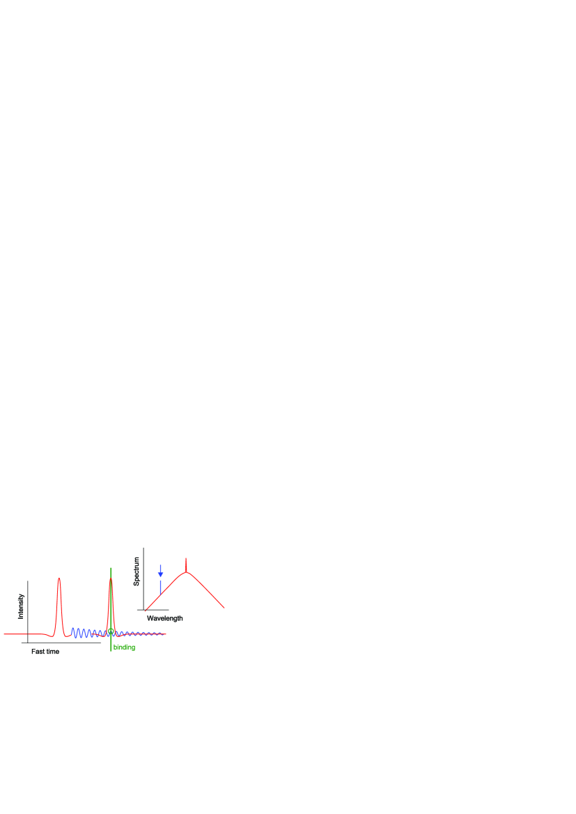
Figure 1: Schematic illustration of the universal temporal CS binding mechanism. A perturbation leads to a sideband in the soliton spectrum (blue arrow). That sideband is associated with an extended oscillatory tail in the temporal intensity profile. An adjacent CS gets trapped by the tail oscillations.

We begin by recalling the early 90s theoretical works of Malomed on the formation of soliton bound states malomed_bound_1991 ; malomed_bound_1993 . In these works, Malomed showed that many forms of nonlinear Schrödinger (NLS) equations, with different perturbations, admit a discrete set of long-range soliton bound states. In every case, bound states arise through excitation, by the perturbation, of a particular frequency in the soliton spectrum (Malomed, concerned with spatial solitons, talked of a particular “wave number”). That frequency is associated with an extended oscillatory tail in the soliton envelope, and when tails of adjacent solitons overlap, this then leads to oscillations in the so-called inter-soliton “effective interaction potential.” Each period of the oscillation constitutes a potential well for a bound state with a specific separation between the solitons. Essentially, bound states arise through the interlocking of the oscillatory tails of adjacent solitons. Long interaction ranges are obtained provided the tail extends over many soliton widths, which is associated with a spectral resonance that is narrow with respect to the soliton bandwidth. In other words, any perturbation that gives rise to a spectral sideband in the soliton spectrum may lead to the formation of long-range bound states. This mechanism is illustrated schematically in Fig. 1.

The standard LLE, in particular, can be seen as a perturbed NLS equation, with extra damping and AC driving terms. Previous analyzes have shown however that, in this case, the oscillatory tails are strongly damped for all values of the cavity detuning but the smallest ones cai_bound_1994 ; barashenkov_bifurcation_1998 ; parra-rivas_interaction_2017 . It is only when the detuning is less than the width of a cavity resonance that substantial oscillations exist and that bound states can be observed in practice, as was demonstrated with spatial CSs schapers_interaction_2000 . For larger values of the detuning, typical of temporal CS experiments, bound states of this nature have not been reported. In the following, we will show that Malomed’s framework can be extended to perturbed forms of the LLE itself, providing a simple way of estimating long-range CS bound state separations. This was also recently studied in parra-rivas_interaction_2017 . In particular, it is already well-known that different forms of perturbations to the LLE, including high-order dispersion milian_soliton_2014-1 ; jang_observation_2014 , mode-crossings herr_mode_2014-1 , and acoustic effects jang_ultraweak_2013 give CSs extended oscillatory tails. Acoustic-mediated bound states of temporal CSs have even been observed in optical fiber rings jang_ultraweak_2013 . These easily fit within our universal description: the spectral sidebands arise through phase modulation of the CS background by the refractive index perturbation created in the fiber core by the acoustic wave.

III Experimental setup

With the aim to provide a clear experimental illustration of the universal concepts outlined above, we will present in the following sections measurements of CS bound states for three different mechanisms. All our experiments are done in fiber ring resonators and we begin by considering the case of DW-induced long-range temporal CS bound states, where the perturbation is due to 3rd-order dispersion. Here we detail the experimental setup for this case. The setups used for the other experiments are very similar: differences will be highlighted in the corresponding Sections.

Our first experiment is performed in a dispersion-managed fiber ring cavity, made up of two different fiber types, similar to that in jang_observation_2014 (see setup in Fig. 2). By carefully adjusting the relative lengths of the two fibers, the average 2nd-order GVD coefficient $\langle\beta_{2}\rangle$ can be selected so as to optimize DW emission. In practice, we used about $95.9$ m of dispersion-shifted fiber (DSF) and $10.3$ m of standard single-mode fiber (SMF). These fibers exhibit, respectively, normal and anomalous GVD at the 1550 nm driving wavelength, with 2nd and 3rd-order GVD coefficients $\beta_{2},\beta_{3}$ and nonlinearity parameters $\gamma$ listed in the caption of Fig. 2. Overall, the average cavity GVD is slightly anomalous at the driving wavelength, $\langle\beta_{2}\rangle\simeq-0.31\ \mathrm{ps^{2}/km}$, with a zero-dispersion wavelength (ZDW) of about 1548 nm. The driving beam is provided by a narrow-linewidth continuous-wave (cw) laser, amplified up to $1.4$ W with an Erbium-doped fiber amplifier (EDFA1), and band-pass filtered (BPF) for amplified spontaneous emission (ASE) noise rejection. It is then coupled into the cavity through a 90/10 fiber coupler. As in jang_observation_2014 , we use the light reflected off the cavity by that coupler as a feedback signal to control and lock the detuning of the driving laser with respect to the cavity resonances. The cavity also includes an optical isolator to avoid stimulated Brillouin scattering leo_temporal_2010 , a 1 % tap coupler to monitor the intracavity field, and a wavelength-division multiplexer (WDM), used for excitation of temporal CSs. The total roundtrip power loss is about 30 %, corresponding to a measured cavity finesse of 17.

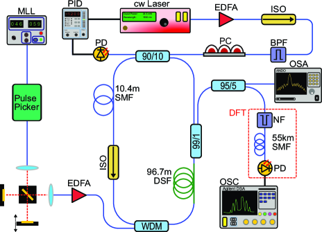
Figure 2: Experimental setup. PC: polarization controller; PD: photo-diode; other acronyms defined in the text. DSF: ${\beta_{2}=1.95}\ \mathrm{ps^{2}/km}$, ${\beta_{3}=0.2\ \mathrm{ps^{3}/km}}$, ${\gamma=2/(\mathrm{W\,km})}$; SMF: ${\beta_{2}=-21.4\ \mathrm{ps^{2}/km}}$, ${\beta_{3}=0.1\ \mathrm{ps^{3}/km}}$, ${\gamma=1.2/(\mathrm{W\,km})}$.

To study CS bound states and their dynamics, we start each measurement by exciting two temporal CSs in close proximity using optical addressing pulses leo_temporal_2010 . The addressing pulses are generated by an external mode-locked laser running at a different wavelength (1532 nm) than the cw driving beam. A single pulse is selected out of the mode-locked pulse train, on request, by a pulse picker. This pulse then passes through an unbalanced Michelson interferometer to create a delayed replica with a controllable separation and both are subsequently amplified to about 10 W peak power (EDFA2) before entering the cavity through the WDM. The pair of addressing pulses circulates for only one roundtrip in the cavity, during which they perturb the cw intracavity field through cross-phase modulation leo_temporal_2010 , before being dumped out by the same WDM. Two temporal CSs eventually emerge (centered at the driving wavelength) from this perturbation. Once the CSs are excited, EDFA2 is switched off and the pulse picker is kept blocked so that no other addressing pulses can affect the system.

To measure the separation between the pair of temporal CSs circulating in the cavity, and to monitor in real time the formation and dynamics of bound states, we send the output light from the tap coupler through 55 km of SMF to perform a real-time dispersive Fourier transform (DFT) wetzel_real-time_2012 ; goda_dispersive_2013 ; runge_coherence_2013 ; herink_resolving_2016 ; katarzyna_real-time_2017 . After traveling through that fiber, the temporal intensity envelope of a CS pair is reshaped into its spectral intensity and this is recorded with a 40 GSample/s digital sampling oscilloscope (OSC). The CS separation is then inferred, roundtrip by roundtrip, from the spectral interference pattern. The measurement is calibrated by comparing the spectrum of a pair of addressing pulses measured with a standard optical spectrum analyser (OSA) and that obtained with the DFT. Note that the cw background on which the pair of temporal CSs sits is not compatible with the DFT scheme. It is thus removed before the 55 km SMF with an extra notch filter (NF; $0.15$ nm bandwidth centered at the 1550 nm driving wavelength).

IV Dispersive wave induced CS bound states

Figure 3(a) shows results from several DFT measurements in our dispersion-managed cavity. The measurements were repeated over many independent realizations with a procedure detailed below in order to identify all possible bound state separations. When the same separation was observed multiple times, the corresponding data are shown in different colors (black, green, and blue curves) in Fig. 3(a) for clarity. Each curve represents an independent recording of the separation of one pair of temporal CSs measured over 42000 roundtrips (plotted every 60 roundtrips). With a roundtrip time $t_{\mathrm{R}}\simeq 0.52\ \mu$s, this corresponds to a relatively large total propagation time (distance) of 22 ms (4500 km), or about 16000 photon lifetimes. It is immediately apparent that the separation between two temporal CSs cannot take arbitrary values: only a discrete set of stable separations are observed, ranging in Fig. 3(a) from $4.2$ ps to 11 ps. Each of these corresponds to a particular bound state of temporal CSs. These bound states are very well defined and reproducible: some of the overlapping measurements have been taken over different days, yet collectively reveal the same set of stable separations. The observed separations are all much larger (7 to 20 times) than the duration of an individual temporal CS, which we estimate to be about $0.6$ ps based on the measured spectrum and numerical modeling [Fig. 3(b)]. We can also see in Fig. 3(a) that, despite environmental noise, the observed separations fluctuate by less than 100 fs even over the very long timescale of our measurements. The underlying binding is thus very robust.

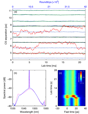
Figure 3: (a) Dynamical evolution of the separation between pairs of temporal CSs. Overlapping data are shown in different colors for clarity (black, green, blue). Red curves are measured in presence of additional ASE noise from EDFA2. (b) Measured (blue) and simulated (purple) spectra of an isolated CS. (c) Observation of a transition between two bound states when a short burst of ASE noise is injected (at time $t\simeq 7$ s).

Note that, in our cavity, we have observed bound states with separations of up to 40 ps (or 66 CS width; not shown). With these larger separations, the bound states are however not as robust: the measured separations fluctuate more, and the overlap of data taken over successive days is not as good as that shown for smaller separations in Fig. 3(a). In these conditions, we also sometimes witness sudden spontaneous changes from one bound state separation to another, when environmental noise is strong enough to push one of the solitons into an adjacent well of the interaction potential. Such spontaneous transitions are never observed in our experiment for separations below 15 ps. The reduced stability of the larger separations can of course be related to the exponentially decaying nature of the soliton tails. To demonstrate that these transitions can be caused by noise, we have monitored the dynamics of bound states in presence of an artificially high level of noise and this is illustrated by the red curves shown in Fig. 3(a). These separation measurements have been obtained with the same DFT technique as the other curves except that EDFA2 was kept powered on (without an input signal) during the measurements, so that all the ASE noise it generates is constantly injected into the cavity through the WDM. Because of the particular dispersion of our cavity, some ASE components are group-velocity matched with the driving beam, guaranteeing efficient noise transfer. As can be seen, the separation between two CSs vary quite erratically in these conditions, and we can observe long portions of the data roughly matching bound states measured without noise, with random transitions between them. A second illustration is provided in Fig. 3(c). Here the pseudo-color plot is made up of a vertical concatenation of oscilloscope recordings of the temporal intensity of the light leaving the cavity over successive roundtrips (bottom to top). The measurement is performed with a 40 GHz sampling oscilloscope and measured with a 65 GHz bandwidth photodiode. A bound state of two CSs with a separation of about 20 ps is initially observed but transitions to a separation of about 12 ps after a short burst of ASE noise is injected into the cavity at time $t\simeq 7$ s. In fact, it is mostly with this method, applied many times, that we have forced the system to visit all the separations that bound states of two CSs can possibly adopt, and accumulated the data shown in black, blue, and green in Fig. 3(a). We must also point out here that the influence of EDFA2 ASE noise on bound states prevent us from directly targeting a specific separation at the excitation stage. Indeed, at that stage, EDFA2 must be powered on to amplify the addressing pulses.

Finally, when looking at all the CS bound states that can be identified in Fig. 3(a), we cannot fail to observe the near periodic arrangement of the allowed separations. This apparent periodicity can be related to Malomed’s picture, in which bound states arise through oscillations in the effective interaction potential. In our case, these oscillations are mainly due to the excitation of a DW peak at 1541 nm, clearly visible on the CS spectrum [Fig. 3(b)]. That frequency component beats with the cw background on which the temporal CSs sit, leading to an extended oscillatory tail milian_soliton_2014-1 ; jang_observation_2014 . The DW peak is separated by about $1.13$ THz from the driving beam, corresponding to tail oscillations with a $0.88$ ps period. That latter figure matches reasonably well with the average $0.75$ ps gap that we observe between allowed separations, thus strongly suggesting that, in our experiment, binding arises primarily through DWs radiated by the CSs. We must point out however that the observed separations are actually not perfectly equidistant: for the data shown in Fig. 3(a), the gaps between allowed bound states range from $0.62$ ps to $0.95$ ps and this spread cannot be attributed to uncertainties in the measurement.

In order to better understand the arrangement of stable separations, we have performed extensive numerical analyzes. In general, we have found that the possible bound state separations are reasonably well predicted by the position of the intensity maxima of the oscillatory tail of an isolated CS. This tail appears to be a good approximation of Malomed’s effective interaction potential malomed_bound_1991 ; malomed_bound_1993 ; parra-rivas_interaction_2017 . We must note that this is also compatible with the well-known fact that CSs are typically trapped at maxima of a modulated background firth_optical_1996 ; jang_temporal_2015 . The oscillatory tail of the CS can be obtained through numerical modeling of the experiment. In our case, because of the not-so-high finesse of the fiber resonator, combined with dispersion management, the temporal CSs breathe over each cavity roundtrip, which breaks the mean-field approximation of the simple LLE jang_observation_2014 . The simplest model that qualitatively accounts for all our observations is a version of the LLE with piecewise-constant $\beta_{2}$, $\beta_{3}$, and $\gamma$ coefficients that mimic our two fiber combination. The validity of this approach has been established in conforti_modulational_2014 . Note that, for simplicity, the cavity losses are still represented by a single distributed coefficient, here $\alpha=0.2$. We seek solutions of this model that are invariant (except for a constant drift) over one full cavity roundtrip using a generalized quasi-Newton (secant) method.

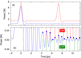
Figure 4: (a) Simulated temporal intensity profiles of an isolated temporal CS (blue) as well as a stable bound state with $7.31$ ps separation (red; shifted vertically for clarity). (b) Vertical enlargement of the tail of the isolated CS. Blue dots denote maxima while red (green) lines indicate the separations of simulated (experimentally observed) bound states, respectively.

The blue curve in Fig. 4(a) shows the simulated temporal intensity profile of an isolated CS, obtained for a driving power of $1.3$ W and a detuning $\delta_{0}=0.57$ rad close to the experimental parameters. The corresponding spectral profile was depicted in Fig. 3(b), and shows good qualitative agreement with experimental observations. Due to 3rd-order dispersion, the CS tail, shown in more details in Fig. 4(b), is strongly asymmetric. In (b), we have highlighted the tail maxima with blue dots and we also show, with red vertical lines, the stable separations allowed between CSs, which have been obtained by looking for the stationary two-soliton solutions of our model [one of which is shown in red in panel (a)]. We can generally observe a good correspondence between the tail maxima and the allowed separations. Differences can be explained by the complexities of the interactions between the two CSs. First, the main peak of the CS is quite wide in comparison to the period of the tail oscillations. As a result, trapping is not simply determined by a maximum. Second, on top of interactions between the main CS peak and the other soliton tail, one must also factor in how the respective tails of the two CSs interlock with each other, which, given the complex shape of the tail, is not trivial to predict. The complex tail shape stems in our case from the rather broad bandwidth of the DW, but also from the additional contribution of the weak Kelly sideband visible at 1563 nm on the spectrum [see Fig. 3(b)] jang_observation_2014 ; luo_resonant_2015 (both are due to departure from the mean-field approximation as explained above). These two spectral features beat with the cw background with non-commensurate frequencies, leading to tail maxima that are not equidistant and whose amplitude does not decrease monotonically away from the soliton main peak. Some shallow maxima arise as a result, and as can be seen in Fig. 4(b), these are not necessarily associated with a stable bound state. Some are also seen to interact with adjacent maxima to affect bound state separations. These mechanisms all contribute to an aperiodic arrangement of the stable bound state separations, compatible with our experimental observations. For comparison, the experimentally measured separations are shown in Fig. 4(b) with the green vertical lines. Given the approximations, and the sensitivity of the model to various parameters, one should not expect perfect agreement. Still, we observe a qualitatively good match.

V Kelly sideband induced CS bound states

The above results provide very strong support for the hypothesis that the experimentally observed temporal CS bound states arise due to DW perturbations. To demonstrate more universally that any perturbation that excites spectral sidebands can lead to distinct bound states, we have performed additional measurements in different cavities that are dominated by different perturbations. These are presented in this Section and the next.

We first consider the case of a fiber cavity of a similar length (100 m) than in our first experiment above but that is made entirely of SMF, and in which higher-order GVD is negligible. In such a cavity, temporal CSs do not excite DWs, as confirmed by a spectral measurement [Fig. 5(a)]. Yet, very weak Kelly sidebands [labeled K in Fig. 5(a)] are still present $3.1$ nm (or 390 GHz) away from the driving laser. The presence of the Kelly sidebands can be explained by the limited finesse of the cavity ($21.5$), corresponding to a relatively large total power loss per roundtrip of about 25 %. This loss causes a periodic oscillation (with a period equal to the cavity roundtrip time) in the power of temporal CSs circulating around the cavity. In turn, this perturbation leads to the excitation of a quasi-phase matched Kelly sideband in the CS spectrum gordon_dispersive_1992 ; kelly_characteristic_1992 ; luo_resonant_2015 .

To test for the presence of CS bound states induced by the Kelly sidebands, we have used the same approach as that in our dispersion-managed cavity. Specifically, we have measured the dynamical evolution of the temporal separation between two CSs over many realizations and this is reported in Fig. 5(b). We still observe a clustering around a discrete set of values, signalling the presence of bound states, but some important differences exist. First, the stable (or quasi-stable) separations are observed to be spaced apart by 2–3 ps, much more than in the dispersion-managed cavity. This is compatible with an interaction potential induced by the Kelly sidebands: $1/390\ \mathrm{GHz}\simeq 2.6$ ps. We note that Kelly-sideband induced binding has also been reported in periodically amplified links and in mode-locked fiber lasers socci_long-range_1999 ; soto-crespo_quantized_2003 . Second, it is apparent that the bound states observed in Fig. 5(b) are much more sensitive to noise, with spontaneous transitions occurring in all realizations every fraction of a second, despite EDFA2 being shut down for these measurements. This can be related to the low amplitude of the Kelly sideband, which leads to a very shallow interaction potential, in comparison to that due to the high amplitude DW observed in the dispersion-managed cavity. Overall, these observations are compatible with the universal binding mechanism introduced in Section II.

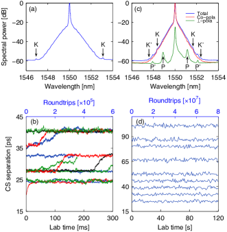
Figure 5: Spectra of a single temporal CS (top) and dynamical evolution of the separation between a pair of such CSs (bottom) in (a), (b) a 100 m-long all-SMF cavity, where CS binding is primarily induced by the Kelly sidebands (K), and (c), (d) in a 315 m-long all-SMF cavity, where binding arises through excitation of orthogonally polarized resonances (P, P’). Notice the different timescales in (b) and (d) (ms versus s).

VI Birefringence induced CS bound states

We now consider additional measurements performed using a longer (315 m) all-SMF cavity (finesse of 19), with results shown in Figs. 5(c)-(d). Preferred separations, hence bound states, are observed in this cavity too but with quite different characteristics than in our two previous experiments described above. We can first note that the bound states revealed by Fig. 5(d) are very robust: no spontaneous transitions are observed even over several minutes. Second, we now observe much larger stable separations, ranging from about 25 to 101 ps. In fact, because of these larger separations, the measurements plotted in Fig. 5(c) have not been obtained with the DFT technique but directly with an optical sampling scope [the same as that used for Fig. 3(c)]. Finally, we must point out the very regular arrangement of the observed bound states, with a constant 7 ps gap between allowed separations (excluding a few missing observations). Again this is larger than reported in the previous Sections, and hints at a different mechanism.

Careful inspection of the temporal CS spectrum for this cavity [blue curve in Fig. 5(c)] reveals several small peaks that could be responsible for the bound states. To gain more insights, we resolved the spectrum into two orthogonally polarized components. We found that the dominant spectral sidebands (P) are associated with light that is orthogonally polarized to the driving beam [green curve in Fig. 5(c)]. Note how these peaks do not register on the co-polarized spectrum (red curve). They are shifted by about $\pm 140$ GHz from the driving frequency (with a slight asymmetry, discussed below) and appear to be responsible for the observed bound states given that $1/140\ \mathrm{GHz}\simeq 7$ ps matches the gap between allowed separations. To confirm that the bound states observed in this cavity are related to polarization and birefringence phenomena, we have added a polarization controller inside our cavity (which is made of standard, non polarization maintaining fiber) to modify the polarization evolution and the overall cavity birefringence. We found that changing the cavity birefringence led to a shift in the cross-polarized sidebands P and higher-order sidebands P’, giving rise to a corresponding change in the spacing between the allowed CS bound state separations. In this cavity, the weaker co-polarized Kelly sidebands, K and K’ on Fig. 5(c), appear to play a negligible role.

To understand better how cross-polarized spectral sidebands can be excited in our cavity, we need to consider in more details the propagation of light along the fiber. All the cavities discussed in this Article are made of fibers with some level of random residual birefringence. The polarization state of the intracavity field evolves randomly around the cavity but there always exist two orthogonal polarization eigenstates for which the polarization state at the end of the roundtrip matches that at the beginning coen_experimental_1998 . These polarization eigenstates are associated with two independent sets of resonances, generally shifted with respect to each other depending on the overall birefringence. In practice, we always carefully align the driving beam polarization with one of these polarization eigenstate. However, on top of linear (random) birefringence, and in the presence of a temporal CS, the peak level of the soliton, and the background on which it sits, will experience different levels of nonlinear polarization rotation as they propagate around the cavity. This leads to some light leaking into the cross-polarized cavity mode. The sidebands P and P’ then simply correspond to components of the associated field that are linearly resonant in the cavity. We note that polarization rotation is essential for this process. In a cavity made up of a polarization-maintaining fiber, with a driving beam polarized along one of its modes, the field does not experience any polarization rotation, and therefore no nonlinear polarization rotation either. We have also identified cross-polarized sidebands in the shorter 100 m-long all-SMF cavity: they are just visible in Fig. 5(a) at an offset of about $2.2$ nm. We infer that the shorter length of that cavity, and of the dispersion-managed cavity as well, does not provide enough differential nonlinear polarization rotation for the polarization sidebands to have a notable influence on the bound states.

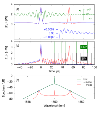
Figure 6: Simulated temporal intensity profiles of the (a) driven ($+$) and (b) cross-polarized ($-$) modes of an isolated temporal CS (blue curves) and that of a particular bound state (red) in a cavity perturbed by fiber birefringence. The green curve in (a) is the ellipticity angle $\Psi$ of the field with respect to the driving field. (b) also shows simulated (black lines) and measured (green lines) allowed bound-state separations. (c) Corresponding spectra.

We have confirmed the above description with numerical simulations based on a new vector mean-field model, Eqs. (A1)–(A2) (see Appendix A for derivation). Isolated and bound-state CS solutions of these equations have been obtained with a generalized Newton method. The temporal intensity profile of an isolated temporal CS is shown as the blue curves in Figs. 6(a) and (b), respectively for the driven ($+$) mode and the cross-polarized ($-$) mode. Notice the difference in scales between these two panels (W versus mW), confirming the perturbative nature of the cross-polarized field. Oscillations with a 7 ps period can be clearly seen in the tail of the cross-polarized field but are also visible when zooming on the co-polarized field [see sub-axis at the bottom right of panel (a)]. The dominant spectral sidebands associated with these tail oscillations are orthogonally polarized to the driving field, as shown on the simulated spectra for the two polarization components [Fig. 6(c)]. Notice how these spectra match very well the experimental observations of Fig. 5(c). We have also calculated the ellipticity angle $\Psi$ of the field with respect to the polarization of the driving field [green curve in panel (a)]. As can be seen, the polarization state varies across the temporal CS, confirming the role of differential nonlinear polarization rotation between the peak and the background of the CS. A particular bound-state is then shown as the red curves in panels (a) and (b), corresponding to a separation of 53 ps. The black lines in panel (b) further locate all the allowed bound state separations, as found with the numerical model. They are found to match well the maxima of the tail of the cross-polarized field of an isolated CS. Panel (b) also shows as green lines the experimental separations, again with a very good agreement with theoretical simulations.

Overall, our analysis confirms that the bound states observed in our 315 m-long SMF cavity, and illustrated in Figs. 5(c)–(d), result from perturbations involving orthogonally polarized light. To the best of our knowledge, this is the first experimental observation of a vector form of temporal CSs. The binding mechanism is also clearly compatible with the universal picture underlying all the other observations reported in this Article.

VII Conclusion

In summary, we have studied the bound states of temporal CSs in fiber ring cavities. We have reported experimental observations of bound states mediated through three different mechanisms involving, respectively, DWs induced by high-order GVD, Kelly sidebands due to the periodic nature of the cavity, and cross-polarized resonances due to random fiber birefringence. Despite the differences between these processes, we have highlighted that the resulting bound states are all underlined by the same universal mechanism: excitation by the CSs of a resonant frequency (or resonant frequencies) that then lead to long oscillatory tails, and a corresponding long-range oscillating interaction potential. This can be interpreted as an extension of Malomed’s work on perturbed NLS soliton bound states malomed_bound_1991 ; malomed_bound_1993 as has also been described recently in the context of the generalized LLE parra-rivas_interaction_2017 . Our measurements clearly highlight that any process generating a spectral sideband may lead to the formation of long-range bound states between CSs, and that several such processes can combine together. This conclusion is compatible with previous observations of acoustic-mediated bound states of temporal CSs jang_ultraweak_2013 and also with recent suggestions that mode-crossings can sometimes explain the stability of multi-soliton states in some Kerr microresonators lamb_stabilizing_2016 . Our observation of DW-induced bound states would similarly explain the high stability multi-soliton states reported in brasch_photonic_2016 and in which mode-crossings are not a dominant feature. Finally, we must point out that our work illustrates the usefulness of the DFT technique for the dynamical study of soliton bound states (see also katarzyna_real-time_2017 ), which could be applicable to other systems in which sub-picosecond resolution is required.

Appendix A

We describe here the model we used to simulate temporal CSs perturbed by the random birefringence of our fiber cavity, and the corresponding bound states (as described in Section VI). This model underlies the results shown in Fig. 6.

To derive our model, we applied the standard mean-field averaging procedure that leads to the scalar LLE haelterman_dissipative_1992 to the set of coupled NLS equations that describes elliptically birefringent fibers as presented in agrawal_nonlinear_2013 [Eqs. (6.1.19)–(6.1.20)]. As usual, the cavity finesse is assumed high enough for the fields not to evolve significantly over one roundtrip, and a corresponding slow time $t$ is introduced to describe the slow evolution of the fields over subsequent roundtrips haelterman_dissipative_1992 . For our cavity, the two polarization modes described by these equations will correspond to the polarization eigenstates of the cavity and will be referred to as $+$ and $-$, where the $+$ mode is the dominant one that is pumped by the external driving laser, whereas the $-$ mode corresponds to the small amount of cross-polarized light. Because the $-$ mode is a small perturbation, we only keep coherent coupling terms that are linear in the corresponding field, $E_{-}$. Overall, this leads to (using the normalization of leo_temporal_2010 )

$$\frac{\partial E_{+}}{\partial t} =\left[-1+i(|E_{+}|^{2}+B|E_{-}|^{2}-\Delta)-i\eta\frac{\partial^{2}}{\partial\tau^{2}}\right]E_{+}$$

$$\qquad+iD\left[q_{\nicefrac{{1}}{{2}}}^{*}E_{+}^{2}E_{-}^{*}+2q_{\nicefrac{{1}}{{2}}}|E_{+}|^{2}E_{-}\right]+S$$ (A1)

$$\frac{\partial E_{-}}{\partial t} =\left[-1+i(|E_{-}|^{2}+B|E_{+}|^{2}-\Delta_{\perp})-i\eta\frac{\partial^{2}}{\partial\tau^{2}}\right.$$

$$\qquad\left.-v_{\perp}\frac{\partial}{\partial\tau}\right]E_{-}+iCq^{*}E_{+}^{2}E_{-}^{*}+iDq_{\nicefrac{{1}}{{2}}}^{*}|E_{+}|^{2}E_{+}$$ (A2)

with $E_{+}=E_{+}(t,\tau)$, $E_{-}=E_{-}(t,\tau)$. Out of the four coherent coupling terms (with coefficients $C$ and $D$) present in these equations, the second one in Eq. (A2) dominates as it only depends on the strong pumped $E_{+}$ mode. In fact, that term acts as a source term for the cross-polarized field $E_{-}$. It is the result of the four-wave mixing product $(+,+)\rightarrow(+,-)$. This source term is essential for our description: without it, Eq. (A2) would be trivially satisfied with $E_{-}=0$ (corresponding to no light in the cross-polarized mode).

We note that, in Eqs. (6.1.19)–(6.1.20) of agrawal_nonlinear_2013 , the two polarization modes are assumed to keep a fixed elliptical state all along the propagation, whereas the ellipticity and orientation of our polarization eigenstates evolve along the cavity due to random birefringence. We take this fact into account by averaging the coupling coefficients $B$, $C$, and $D$ (Eq. (6.1.21) of agrawal_nonlinear_2013 ) over all possible modal ellipticities, leading to $B=1.3$, $C=0.2$, $D=0.13$. This approach is different from the usual Manakov approximation and that corresponds to a full average of polarization coupling terms agrawal_nonlinear_2013 . In the case of our cavity, the average is not complete, because the polarization state of the cavity polarization eigenstates are restored periodically at the end of each roundtrip. This leads to a net leak of power from one mode to the other that accumulates over subsequent roundtrips, as embodied by the source term of Eq. (A2) described above. The incomplete polarization averaging also makes necessary to take into account the difference in group velocities between the two modes represented by the first-order fast time derivative, with $v_{\perp}$ the differential group delay accumulated over one roundtrip.

Other symbols of Eqs. (A1)–(A2) are as follows. As in the usual LLE, $\tau$ is the fast-time that describes the temporal profile of the fields, $\eta$ is the sign of the GVD coefficient $\beta_{2}$ ($\eta=-1$ here, corresponding to anomalous dispersion), and $S$ is the driving strength. $\Delta$ and $\Delta_{\perp}$ measure the detuning between the driving laser frequency and the closest resonance of, respectively, the driven ($+$) and cross-polarized ($-$) modes. The two sets of resonances are generally shifted with respect to each other ($\Delta\neq\Delta_{\perp}$) because of birefringence, and the detunings are related to the difference in cavity roundtrip phase shift (at the driving frequency) between the two polarization modes, $\phi_{0+}-\phi_{0-}=\Delta\phi_{0}=\alpha(\Delta_{\perp}-\Delta)+2k\pi$ (where $\alpha=\pi/\mathcal{F}\simeq 0.165$, with $\mathcal{F}\simeq 19$ the cavity finesse). $\Delta\phi_{0}$ is needed to determine the parameters $q=\mathrm{sinc}(\Delta\phi_{0})e^{-i\Delta\phi_{0}}$ and $q_{\nicefrac{{1}}{{2}}}=\mathrm{sinc}(\Delta\phi_{0}/2)e^{-i\Delta\phi_{0}/2}$ that represent the effect of the phase-mismatch of the various four-wave mixing products. We note that when the two sets of resonances match ($\Delta=\Delta_{\perp}$), we have $q=q_{\nicefrac{{1}}{{2}}}=0$, and there is no net polarization coupling (even with a multiple of $2\pi$ phase shift).

The normalized driving power $X=S^{2}\simeq 4.7$ and detuning $\Delta\simeq 3$ are determined from corresponding settings of the experiment. $\Delta_{\perp}$ and the differential group delay $v_{\perp}$ can then be found from the positions of the first order cross-polarized spectral sidebands [$P$ in Fig. 5(c)] which satisfy the resonance condition $\Omega_{\mathrm{P}}^{2}-v_{\perp}\Omega_{\mathrm{P}}+\Delta_{\perp}=0$ (with $\Omega_{\mathrm{P}}$ the angular frequency shift of the sidebands with respect to the driving frequency). We found $\Delta_{\perp}\simeq-16$ and $v_{\perp}\simeq-0.1$. Clearly, $v_{\perp}$ is responsible for the slight asymmetry in the location of the spectral sidebands. Yet this quantity is very small: it corresponds to a differential group delay of $-75\ \mathrm{fs/roundtrip}$ in real units and indicates that the polarization average is close to complete. We note that we can only determine $\Delta\phi_{0}$ to within modulo $2\pi$ with this method. After some trials, we chose an extra $2\pi$ shift in roundtrip phase ($k=1$) for our simulation as it led to reasonably good agreement with observations. Larger values of $k$ simply lead to weaker coupling and weaker cross-polarized sidebands.

Funding Information

Marsden fund of the Royal Society of New Zealand; Rutherford Discovery Fellowships of the Royal Society of New Zealand. Julien Fatome also acknowledges the financial support from the European Research Council (ERC starting grant PETAL #306633) and the Conseil Régional de Bourgogne Franche-Comté (International Mobility Program) which has allowed him to visit The University of Auckland to contribute to this work.

References

- (1) F. Leo, S. Coen, P. Kockaert, S.-P. Gorza, Ph. Emplit, and M. Haelterman, “Temporal cavity solitons in one-dimensional Kerr media as bits in an all-optical buffer,” Nature Photon. 4, 471–476 (2010).
- (2) J. K. Jang, M. Erkintalo, S. Coen, and S. G. Murdoch, “Temporal tweezing of light through the trapping and manipulation of temporal cavity solitons,” Nature Commun. 6, 7370 (2015).
- (3) J. K. Jang, M. Erkintalo, J. Schröder, B. J. Eggleton, S. G. Murdoch, and S. Coen, “All-optical buffer based on temporal cavity solitons operating at 10 Gb/s,” Opt. Lett. 41, 4526–4529 (2016).
- (4) S. Coen, H. G. Randle, T. Sylvestre, and M. Erkintalo, “Modeling of octave-spanning Kerr frequency combs using a generalized mean-field Lugiato-Lefever model,” Opt. Lett. 38, 37–39 (2013).
- (5) T. Herr, V. Brasch, J. D. Jost, C. Y. Wang, N. M. Kondratiev, M. L. Gorodetsky, and T. J. Kippenberg, “Temporal solitons in optical microresonators,” Nature Photon. 8, 145–152 (2014).
- (6) X. Yi, Q.-F. Yang, K. Y. Yang, M.-G. Suh, and K. Vahala, “Soliton frequency comb at microwave rates in a high-Q silica microresonator,” Optica 2, 1078–1085 (2015).
- (7) C. Joshi, J. K. Jang, K. Luke, X. Ji, S. A. Miller, A. Klenner, Y. Okawachi, M. Lipson, and A. L. Gaeta, “Thermally controlled comb generation and soliton modelocking in microresonators,” Opt. Lett. 41, 2565–2568 (2016).
- (8) K. E. Webb, M. Erkintalo, S. Coen, and S. G. Murdoch, “Experimental observation of coherent cavity soliton frequency combs in silica microspheres,” Opt. Lett. 41, 4613–4616 (2016).
- (9) T. J. Kippenberg, R. Holzwarth, and S. A. Diddams, “Microresonator-based optical frequency combs,” Science 332, 555–559 (2011).
- (10) L. A. Lugiato and R. Lefever, “Spatial dissipative structures in passive optical systems,” Phys. Rev. Lett. 58, 2209–2211 (1987).
- (11) M. Haelterman, S. Trillo, and S. Wabnitz, “Dissipative modulation instability in a nonlinear dispersive ring cavity,” Opt. Commun. 91, 401–407 (1992).
- (12) A. B. Matsko, A. A. Savchenkov, W. Liang, V. S. Ilchenko, D. Seidel, and L. Maleki, “Mode-locked Kerr frequency combs,” Opt. Lett. 36, 2845–2847 (2011).
- (13) F. Leo, L. Gelens, Ph. Emplit, M. Haelterman, and S. Coen, “Dynamics of one-dimensional Kerr cavity solitons,” Opt. Express 21, 9180–9191 (2013).
- (14) Y. K. Chembo and C. R. Menyuk, “Spatiotemporal Lugiato-Lefever formalism for Kerr-comb generation in whispering-gallery-mode resonators,” Phys. Rev. A 87, 053852/1–4 (2013).
- (15) P. Parra-Rivas, D. Gomila, M. A. Matías, S. Coen, and L. Gelens, “Dynamics of localized and patterned structures in the Lugiato-Lefever equation determine the stability and shape of optical frequency combs,” Phys. Rev. A 89, 043813/1–12 (2014).
- (16) W. J. Firth and A. J. Scroggie, “Optical bullet holes: Robust controllable localized states of a nonlinear cavity,” Phys. Rev. Lett. 76, 1623–1626 (1996).
- (17) T. Ackemann, W. J. Firth, and G.-L. Oppo, “Chapter 6: Fundamentals and applications of spatial dissipative solitons in photonic devices,” Adv. At. Mol. Opt. Phys. 57, 323–421 (2009).
- (18) P. Parra-Rivas, D. Gomila, P. Colet, and L. Gelens, “Interaction of solitons and the formation of bound states in the generalized Lugiato-Lefever equation,” submitted to Eur. Phys. J. D (2017).
- (19) J. K. Jang, M. Erkintalo, S. G. Murdoch, and S. Coen, “Bound states of temporal cavity solitons,” in “Nonlinear Photonics, NP’2014,” (Optical Society of America, Barcelona, Spain, July 27-31, 2014), OSA Technical Digest (online), pp. 2 pages, poster JM5A.59. Accepted:.
- (20) P. Del’Haye, A. Coillet, W. Loh, K. Beha, S. B. Papp, and S. A. Diddams, “Phase steps and resonator detuning measurements in microresonator frequency combs,” Nat Commun 6, 5668 (2015).
- (21) V. Brasch, M. Geiselmann, T. Herr, G. Lihachev, M. H. P. Pfeiffer, M. L. Gorodetsky, and T. J. Kippenberg, “Photonic chip–based optical frequency comb using soliton Cherenkov radiation,” Science 351, 357–360 (2016).
- (22) X. Yi, Q.-F. Yang, K. Y. Yang, and K. Vahala, “Active capture and stabilization of temporal solitons in microresonators,” Opt. Lett. 41, 2037–2040 (2016).
- (23) E. S. Lamb, D. C. Cole, P. Del’Haye, K. Y. Yang, K. J. Vahala, S. A. Diddams, and S. B. Papp, “Stabilizing multiple solitons in Kerr microresonator frequency combs,” in “Conference on Lasers and Electro-Optics,” (Optical Society of America, 2016), p. SW1E.3.
- (24) C. Milián and D. V. Skryabin, “Soliton families and resonant radiation in a micro-ring resonator near zero group-velocity dispersion,” Opt. Express 22, 3732–3739 (2014).
- (25) J. K. Jang, M. Erkintalo, S. G. Murdoch, and S. Coen, “Observation of dispersive wave emission by temporal cavity solitons,” Opt. Lett. 39, 5503–5506 (2014).
- (26) B. Wetzel, A. Stefani, L. Larger, P. A. Lacourt, J. M. Merolla, T. Sylvestre, A. Kudlinski, A. Mussot, G. Genty, F. Dias, and J. M. Dudley, “Real-time full bandwidth measurement of spectral noise in supercontinuum generation,” Sci. Rep. 2, 882 (2012).
- (27) K. Goda and B. Jalali, “Dispersive Fourier transformation for fast continuous single-shot measurements,” Nat Photon 7, 102–112 (2013).
- (28) A. F. J. Runge, C. Aguergaray, N. G. R. Broderick, and M. Erkintalo, “Coherence and shot-to-shot spectral fluctuations in noise-like ultrafast fiber lasers,” Opt. Lett. 38, 4327–4330 (2013).
- (29) G. Herink, B. Jalali, C. Ropers, and D. R. Solli, “Resolving the build-up of femtosecond mode-locking with single-shot spectroscopy at 90 MHz frame rate,” Nat Photon 10, 321–326 (2016).
- (30) B. A. Malomed, “Bound solitons in the nonlinear Schrödinger–Ginzburg-Landau equation,” Phys. Rev. A 44, 6954–6957 (1991).
- (31) B. A. Malomed, “Bound states of envelope solitons,” Phys. Rev. E 47, 2874–2880 (1993).
- (32) D. Cai, A. R. Bishop, N. Grønbech-Jensen, and B. A. Malomed, “Bound solitons in the AC-driven, damped nonlinear Schrödinger equation,” Phys. Rev. E 49, 1677–1679 (1994).
- (33) I. V. Barashenkov, Y. S. Smirnov, and N. V. Alexeeva, “Bifurcation to multisoliton complexes in the AC-driven, damped nonlinear Schrödinger equation,” Phys. Rev. E 57, 2350–2364 (1998).
- (34) B. Schäpers, M. Feldmann, T. Ackemann, and W. Lange, “Interaction of localized structures in an optical pattern-forming system,” Phys. Rev. Lett. 85, 748–751 (2000).
- (35) T. Herr, V. Brasch, D. Jost, J. I. Mirgorodskiy, G. Lihachev, L. Gorodetsky, M. and J. Kippenberg, T. “Mode spectrum and temporal soliton formation in optical microresonators,” Phys. Rev. Lett. 113, 123901 (2014).
- (36) J. K. Jang, M. Erkintalo, S. G. Murdoch, and S. Coen, “Ultraweak long-range interactions of solitons observed over astronomical distances,” Nature Photon. 7, 657–663 (2013).
- (37) K. Katarzyna, K. Nithyanandan, U. Andral, P. Tchofo-Dinda, and P. Grelu, “Real-time observation of dissipative optical soliton molecular motions,” arXiv 1702.01161 (2017).
- (38) M. Conforti, A. Mussot, A. Kudlinski, and S. Trillo, “Modulational instability in dispersion oscillating fiber ring cavities,” Opt. Lett. 39, 4200–4203 (2014).
- (39) K. Luo, Y. Xu, M. Erkintalo, and S. G. Murdoch, “Resonant radiation in synchronously pumped passive Kerr cavities,” Opt. Lett. 40, 427–430 (2015).
- (40) J. P. Gordon, “Dispersive perturbations of solitons of the nonlinear Schrödinger equation,” J. Opt. Soc. Am. B 9, 91 (1992).
- (41) S. M. J. Kelly, “Characteristic sideband instability of periodically amplified average soliton,” Electron. Lett. 28, 806–807 (1992).
- (42) L. Socci and M. Romagnoli, “Long-range soliton interactions in periodically amplified fiber links,” J. Opt. Soc. Am. B 16, 12–17 (1999).
- (43) J. M. Soto-Crespo, N. Akhmediev, P. Grelu, and F. Belhache, “Quantized separations of phase-locked soliton pairs in fiber lasers,” Opt. Lett. 28, 1757–1759 (2003).
- (44) S. Coen, M. Haelterman, Ph. Emplit, L. Delage, L. M. Simohamed, and F. Reynaud, “Experimental investigation of the dynamics of a stabilized nonlinear fiber ring resonator,” J. Opt. Soc. Am. B 15, 2283–2293 (1998).
- (45) G. P. Agrawal, Nonlinear Fiber Optics (Academic Press, 2013), 5th ed.