The Reversibility Error Method (REM): a new, dynamical fast indicator for planetary dynamics

Abstract

We describe the Reversibility Error Method (REM) and its applications to planetary dynamics. REM is based on the time-reversibility analysis of the phase-space trajectories of conservative Hamiltonian systems. The round-off errors break the time reversibility and the displacement from the initial condition, occurring when we integrate it forward and backward for the same time interval, is related to the dynamical character of the trajectory. If the motion is chaotic, in the sense of non-zero maximal Characteristic Lyapunov Exponent (mLCE), then REM increases exponentially with time, as $\exp\lambda t$, while when the motion is regular (quasi-periodic) then REM increases as a power law in time, as $t^{\alpha}$, where $\alpha$ and $\lambda$ are real coefficients. We compare the REM with a variant of mLCE, the Mean Exponential Growth factor of Nearby Orbits (MEGNO). The test set includes the restricted three body problem and five resonant planetary systems: HD 37124, Kepler-60, Kepler-36, Kepler-29 and Kepler-26. We found a very good agreement between the outcomes of these algorithms. Moreover, the numerical implementation of REM is astonishing simple, and is based on solid theoretical background. The REM requires only a symplectic and time-reversible (symmetric) integrator of the equations of motion. This method is also CPU efficient. It may be particularly useful for the dynamical analysis of multiple planetary systems in the Kepler sample, characterized by low-eccentricity orbits and relatively weak mutual interactions. As an interesting side-result, we found a possible stable chaos occurrence in the Kepler-29 planetary system.

1 Introduction

During the past few years, the space mission Kepler has discovered more than 550 multi-planet compact systems with relatively small-mass super-Earth planets. This has brought new understanding of the orbital architectures and the long-term evolution of extrasolar systems. Short period exoplanets in multi-planet systems raise a puzzling scenario of their formation and evolution. In such near-resonant or resonant compact configurations, wide ranges of gravitational interactions between planets are expected and chaotic dynamics due to resonance overlap (Chirikov, 1979; Wisdom, 1983; Quillen, 2011) may lead to close encounters (Chambers et al., 1996; Chatterjee et al., 2008) and self-disrupting systems (Chambers, 1999). The mean motion resonances (MMRs) and secular resonances are the crucial factors for the orbital evolution of compact planetary systems and determine their long-term stability (Morbidelli, 2002; Guzzo, 2005; Quillen, 2011).

A dynamical analysis of the observational data is often a challenge by itself. Short baseline, sparse sampling and noisy measurements introduce uncertainties and biases of the inferred orbital parameters. Uncertainties of the best-fitting models may cover qualitatively different orbital configurations. Just to mention a few examples, we recall here planetary systems of Kepler-223 (Mills et al., 2016), HD 202206 (Couetdic et al., 2010), $\nu$-Octantis (Ramm et al., 2016; Goździewski et al., 2013), HR 8799 (Marois et al., 2010; Goździewski & Migaszewski, 2014), HD 47366 (Sato et al., 2016). The dynamical analysis of the best-fitting planetary models has become a standard approach. For compact, resonant, strongly interacting systems, the optimization of observational models may benefit from implicit constraints of the dynamical stability (i.e., Goździewski et al., 2008; Goździewski & Migaszewski, 2014).

Analysis of such problems makes use of the so called fast dynamical indicators which are common for the dynamical systems theory. These numerical techniques make it possible to analyse efficiently large volumes of the phase/parameter-space. The fast indicators are developed to distinguish between stable and unstable (regular or chaotic) motions on the basis of relatively short arcs of phase-space trajectories of their dynamical systems. The most common tools in this class are algorithms based on the maximal Characteristic Lyapunov Exponent (mLCE, Benettin et al., 1980), the Fast Lyapunov Indicator (FLI, Froeschlé et al., 1997), the Mean Exponential Growth factor of Nearby Orbits (MEGNO, Cincotta & Simó, 2000; Cincotta et al., 2003; Cincotta & Giordano, 2016), the Smaller/Generalized Alignment Index (SALI and GALI, Souchay & Dvorak, 2010), the Orthogonal Fast Lyapunov Indicator (OFLI and OFLI2, Barrio, 2016) as well as on a few variants of the refined Fourier frequency analysis, like the Numerical Analysis of Fundamental Frequencies (NAFF, Laskar, 1990; Laskar et al., 1992), the Frequency Modified Fourier Transform (FMFT, Šidlichovský & Nesvorný, 1996), and the Spectral Number (SN, Michtchenko & Ferraz-Mello, 2001).

The Hamiltonian formulation of the equations of motion makes it possible to construct symplectic integrators (SI) which preserve the geometrical properties of the Hamiltonian flow (Hairer et al., 2006). Regarding the planetary $N$-body problem, SI are CPU efficient and reliable methods for long-term integration intervals that have brought a breakthrough in this field (Wisdom & Holman, 1991). Remarkably, SI are usually time-reversible (symmetric) schemes like the second order leapfrog (Yoshida, 1990; Hairer et al., 2006).

A numerical breakup of the time-reversibility has been proved to be a sufficient condition to detect chaotic trajectories in the phase-space (Aarseth et al., 1994; Lehto et al., 2008; Faranda et al., 2012). Unlike regular orbits, an ergodic motion is expected to result in large displacements of the initial condition ${\boldsymbol{x}}_{0}$ after the forward and backward integration. Since SI are equivalent to symplectic maps, it makes it possible to determine and rigorously prove analytic properties of a numerical approach based on this idea developed in a series of papers (Turchetti et al., 2010a, b; Faranda et al., 2012; Panichi et al., 2016).

This relatively new dynamical fast indicator, called Reversibility Error Method (REM from hereafter), is based on the time reversibility of the ordinary differential equations (ODE). Rather than studying the divergence of phase-space trajectories with the shadow orbits algorithm or with the variational equations of the equations of motion (i.e., Benettin et al., 1980), REM relies on integrating the same orbit forward and backward with a time-reversible (symmetric) numerical integrator. A phase-space orbit may be classified w.r.t. the growth rate of the global error due to the accumulation of the round-off errors occurring in each integration step (forward and backward). If the orbit is regular, in the sense of mLCE, the accumulation of numerical errors develops as a power law in time, $\sim t^{\alpha}$, while for mLCE-unstable trajectory this effect is exponentially amplified by its chaotic nature, $\sim\exp\lambda t$, where $\alpha$ and $\lambda$ are real coefficients.

Numerical applications of REM to low-dimensional dynamical systems has revealed that it could be a sensitive and CPU efficient numerical fast indicator. Given its similarity to mLCE (Turchetti et al., 2010a; Faranda et al., 2012), the advantage is a great simplicity of numerical implementation.

The main aim of this paper is to introduce the REM algorithm for studying dynamical properties of compact systems of Earth-like planets discovered by the Kepler mission. These systems are resonant or near-resonant, however with orbits in small and moderate eccentricity range. We intend to show that REM is an effective and precise fast indicator for this class of systems as common mLCE methods.

The paper is structured as follows. After the Introduction, in Sect. 2, we briefly introduce the fast indicators REM, MEGNO and FMFT as reference tools. Next, based on the perturbation criterion for near-integrable dynamical systems, we select a few examples to compare these indicators. Section  3 is devoted to a brief presentation of these dynamical systems. We recall a simple Hamiltonian system which exhibits the Arnold diffusion and the restricted three body problem. The main target of our work are compact 3-planet systems, HD 37124 and Kepler-60, as well as 2-planet low-order MMR systems, Kepler-29, Kepler-26 and Kepler-36, which may be examples of “typical” near-resonant or resonant pairs of Super-Earth planets in the Kepler sample. In Section 4 we present the results of numerical experiments with the fast indicators. Section  5 is devoted to numerical integrators, numerical accuracy and CPU efficiency of the REM. After Conclusions (Sect. 6), Appendix A shows a detailed theoretical background of this approach by comparing the Lyapunov error, due to the initial displacement, with the forward and reversibility errors due to random perturbations along the orbit.

2 Dynamical fast indicators

The analysis of the long-term evolution of planetary systems is based on various analytic theories and on the direct, numerical integration of the equations of motion (e.g., Wisdom & Holman, 1991; Chambers, 1999; Laskar & Robutel, 2001; Ito & Tanikawa, 2002; Laskar & Gastineau, 2009). Besides these approaches, fast indicators are common tools to analyse the structure of chaotic and quasi-periodic motions in the phase-space. Here, we briefly describe REM and MEGNO, which may be considered as mLCE-related fast indicators, and a variant of the spectral algorithms, FMFT.

2.1 Reversibility Error Method (REM)

The formal derivation of the REM for linear maps, its properties and connection with the mLCE are presented in (Panichi et al., 2016). For Hamiltonian systems studied in this paper, which split into two individually integrable terms, we prove analytical properties of the reversibility error and charterise its changes for different regimes of motion. A detailed introduction and analysis of REM for nonlinear symplectic maps, which generalize the results in (Panichi et al., 2016), are given in Appendix  A. Here we present only a brief and “practical” introduction.

Given an autonomous Hamiltonian system ${\cal H}$, the phase-space evolution of its solutions can be defined as the symplectic map $\bm{\mathsfit{M}}({\boldsymbol{x}})$ which iterates the conjugate variables ${\boldsymbol{x}}$,

$${\boldsymbol{x}}_{n}=\bm{\mathsfit{M}}({\boldsymbol{x}}_{n-1}),\quad n=1,\ldots,$$ (1)

where $n$ is the iteration index, and ${\boldsymbol{x}}_{0}$ is the initial condition, ${\boldsymbol{x}}_{0}\equiv{\boldsymbol{x}}(t=t_{0})$. We introduce a perturbed map $\bm{\mathsfit{M}}_{\gamma}({\boldsymbol{x}})$ where $\gamma$ is a measure of the perturbation amplitude. For a generic Hamiltonian map, the reversibility error at iteration $n$ is (see Appendix A),

$$d_{n}^{\mbox{\scriptsize(R)}}=\sqrt{\langle{}\left\|\bm{\mathsfit{M}}_{\gamma}^{-n}(\bm{\mathsfit{M}}_{\gamma}^{n}({\boldsymbol{x}}_{0}))-{\boldsymbol{x}}_{0}\right\|^{2}{}\rangle},$$ (2)

where “${-n}$” denotes the $n$-th backward iteration and “$n$” the $n$-th forward iteration of $\bm{\mathsfit{M}}_{\gamma}$. The kind of perturbation and its amplitude are quite arbitrary: for Hamiltonian flows it may be the white noise, for a symplectic map it may be a random additive perturbation or the round-off error due to finite machine precision.

To apply Eq. 2 numerically, we must guarantee that the map is invertible (Faranda et al., 2012; Panichi et al., 2016). For a numerical integrator affected by a round-off error of amplitude $\gamma$, we change Eq. 2 into

$$d_{n}^{(R)}=\sqrt{\|\Phi^{\cal H}_{\gamma,-nh}\circ\Phi^{\cal H}_{\gamma,nh}({\boldsymbol{x}}_{0})-{\boldsymbol{x}}_{0}\|^{2}},$$ (3)

where $\Phi^{\cal H}_{nh}$ denotes an SI scheme advancing the initial condition from $t=0$ to $t=nh\equiv T$, where $h$ is the integration step. The scheme is time reversible, so that

$$\Phi^{\cal H}_{-h}\circ\Phi^{\cal H}_{h}\equiv id,$$ (4)

for one integration step $h$ (Hairer et al., 2006). (Symplectic integrators may be not time-reversible integrators and vice-versa). The reversibility condition is lost for maps with the round-off and/local errors $\Phi^{\cal H}_{\gamma,nh}$. Note that in Eq. 3, we dropped the average which appears in Eq. 2, since unlikely for random perturbation, just a single realization of round-off errors is available.

The reversibility error is therefore the norm of the displacement from a selected initial condition in the phase-space, after integrating the equations of motion forward and back for the same time interval $T=nh$ (the number of steps).

Most symplectic integrator schemes $\Phi^{\cal H}_{h}$ used in practice are symmetric by design. For instance, if the Hamiltonian may be split into two terms, ${\cal H}={\cal H}_{A}+{\cal H}_{B}$, which are individually integrable, then the second order leapfrog scheme

$$\Phi^{\cal H}_{h}\equiv\phi_{h/2}^{\cal A}\circ\phi_{h}^{\cal B}\circ\phi_{h/2}^{\cal A},$$ (5)

is composed of symmetric flows $\phi^{\cal A}_{t}$ and $\phi^{\cal B}_{t}$ for Hamiltonians ${\cal H}_{A}$ and ${\cal H}_{B}$, respectively. This time-reversible scheme results in the local error $O(h^{3})$.

A great advantage of the leapfrog is that it may be easily generalized to higher order schemes, as shown by Yoshida (1990). Here, we apply the 4th order integrator of Yoshida, as well as a family of symmetric and symplectic integrators called SABA_n and SBAB_n (Laskar & Robutel, 2001).

A typical behaviour of REM for chaotic and regular phase-space trajectories is illustrated in Fig. 1. This shows the time-evolution of the REM computed for each individual planet in the three-planet system HD 37124 (see Sect. 3.4.1 for details). The integration has been performed for a forward interval of 50 kyrs, and with the 4th order SABA₄ scheme with fixed time-step equal to 1 day. For each planet, the REM increases following a power law w.r.t. the integration time for a stable solution. We note that the deviation must increase due to the accumulation of the numerical round-off and, possibly, due to the local truncation error. We would like to note that the error with respect to exact flow depends on both the truncation and the round-off errors and estimates are difficult unless one of them is dominant. For the chaotic orbit, the reversibility error increase rate has an exponential character. The crucial point is that the final REM deviations differ by $\sim 7$ orders of magnitude, and the orbits signatures could be easily distinguished one from each other.

We make use of this property in Sect. 4 by constructing dynamical maps in planes of selected orbital and dynamical parameters. The REM values are classified through their character of time-variability and relative ranges. We note that a very similar calibration is known for the FLI (Froeschlé et al., 1997) or the mLCE itself, since these indicators do not offer an absolute measure of the instability degree in finite intervals of time.

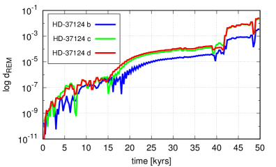
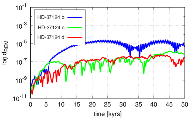
Figure 1: Time evolution of REM for the HD 37124 planetary system. The top panel is for an unstable configuration, the bottom panel is for a stable, quasi-periodic solution. The REM is computed for each orbit separately, and marked with different colours (grey shades). The innermost planet (black, blue in the online version) appears to be most influenced by the chaotic system, due to large value of REM ($10^{-5}$) at the end of the total integration interval of $2\times 50$ kyrs. The second planet (light-grey, green in the online version) and the third one (grey, red in the online version) exhibit slower increase of REM which reach $10^{-7}$ at the end of the simulation. For the unstable configuration, the REM components increase much faster, and they reach $0.1$, a few orders of magnitude larger value than for the regular model.

2.2 Mean Exponential Growth factor of Close Orbits

Together with the evolution of the phase-space trajectory, Eq. 1, it is possible to propagate an initial displacement vector ${\boldsymbol{\eta}}$ with the tangent map $D\bm{\mathsfit{M}}$ defined as $D\bm{\mathsfit{M}}_{ij}=\partial\bm{\mathsfit{M}}_{i}/\partial{\boldsymbol{x}}_{j}$, $i,j=1,\ldots 2N$, and $N$ is the number of the degrees of freedom,

$${\boldsymbol{\eta}_{n}}=D\bm{\mathsfit{M}}({\boldsymbol{x}}_{n-1})\,{\boldsymbol{\eta}}_{n-1},\quad n>0.$$ (6)

(See also Appendix A). This discretization means solving the Hamiltonian ODE system including the equations of motion and the variational equations. The evolution of ${\boldsymbol{\eta}}(t)$ determines the maximal Characteristic Lyapunov Exponent (mLCE, Benettin et al., 1980)

$$\lambda\equiv\lim_{n\rightarrow\infty}\frac{1}{n}\log\frac{\|{\boldsymbol{\eta}}_{n}\|}{\|{\boldsymbol{\eta}}_{0}\|},\quad{\boldsymbol{\eta}}_{0}\equiv{{\boldsymbol{\eta}}}(t_{0}),$$

or its close relatives, like the Fast Lyapunov Indicator (FLI, Froeschlé et al., 1997) and the Mean Exponential Growth factor of Nearby Orbits (MEGNO, Cincotta & Simó, 2000; Cincotta et al., 2003).

Though MEGNO has been primarily defined for continuous ODEs, here we choose its formulation for maps, consistent with REM formalism in other parts of this paper. It reads (Cincotta et al., 2003)

$$Y_{n}=\frac{2}{n}\sum_{k=1}^{n}k\,\ln\frac{\|{\boldsymbol{\eta}}_{k}\|}{\|{\boldsymbol{\eta}}_{k-1}\|},\quad\langle Y\rangle_{n}=\frac{1}{n}\sum_{k=1}^{n}Y_{k},$$ (7)

where ${\boldsymbol{\eta}_{k}}$ is the tangent vector at step $k$, ${\boldsymbol{\eta}}_{0}$ is random initial vector, $\|{\boldsymbol{\eta}}_{0}\|=1$, and $n$ is the number of steps. To propagate the MEGNO map Eqs. 7 for $N$-body planetary problem, we implemented (Goździewski et al., 2008) a symplectic tangent map (Mikkola & Innanen, 1999) that solves the equations of motion and the variational equations simultaneously.

The discrete map $\langle Y\rangle_{n}$ asymptotically tends to

$$\langle Y\rangle_{n}=an+b,$$

with $a=0,b=2$ for a quasi-periodic orbit, $a=b=0$ for a stable, isochronous periodic orbit, and $a=\lambda/2,\,b=0$ for a chaotic orbit, where $\lambda$ is the mLCE approximation. Thus we can estimate the mLCE on a finite time interval by fitting the straight line to $\langle Y\rangle_{n}$ (see Cincotta et al., 2003, for details).

Since MEGNO is essentially equivalent to FLI (Mestre et al., 2011), and makes it possible to estimate the mLCE values, we consider it a well tested and a representative fast indicator in the large family of variational algorithms (Barrio et al., 2009).

In general, the fixed step size symplectic integrators cannot be used for configurations suffering from close encounters due to eccentric orbits. In such cases, we use the MEGNO formulation for ODEs (Cincotta & Simó, 2000) with adaptive-step Bulirsch-Stoer-Gragg extrapolation method (Hairer et al., 2006, ODEX code).

2.3 Frequency modified Fourier Transform

For one example system tested in this paper (Kepler-29), we used the (FMFT, Šidlichovský & Nesvorný, 1996), which is classified as a spectral algorithm. We analyse the time series of heliocentric Keplerian elements ${\cal S}_{i}=\{a_{i}(t_{k})\exp(\mbox{i}\lambda_{i}(t_{k})\}$ of planets $i=\mbox{b},\mbox{c},\mbox{d},\ldots$ and $k=1,\ldots 2^{N}$, where $N$ is the number of samples. These elements are inferred from canonical Poincaré coordinates through usual two-body orbit transformation (Morbidelli, 2002). For a near-integrable planetary system, the FMFT transform of such series provides one of the fundamental, canonical frequencies, namely the proper mean motion, $n_{i}$ associated with the largest amplitude $a^{0}_{i}$ (the proper mean motion) of signal ${\cal S}_{i}$, for each of its planets.

We are interested in the diffusion of these proper mean motions, hence for each planet we define a coefficient of the diffusion of fundamental frequencies (Robutel & Laskar, 2001):

$$\sigma_{f}=\frac{n_{\Delta t\in[0,T]}}{n_{\Delta t\in[T,2T]}}-1,\quad T=Nh~{},$$

where $h$ is the sampling step. If the frequencies for time intervals $\Delta t\in[0,T]$ and $\Delta t\in[T,2T$] do not change, the motion is quasi-periodic, while $\sigma_{f}$ different from zero indicates a chaotic solution. This fast indicator has been proved to be very sensitive for chaotic motions (Robutel & Laskar, 2001; Šidlichovský & Nesvorný, 1996).

3 Between strong and weak perturbations

We consider a near-integrable Hamiltonian system

$${\cal H}({\boldsymbol{I}},{\boldsymbol{\theta}})={\cal H}_{0}({\boldsymbol{I}})+\epsilon{\cal H}_{1}({\boldsymbol{I}},{\boldsymbol{\theta}}),\quad\epsilon\in[0,1),$$ (8)

composed of the integrable term ${\cal H}_{0}({\boldsymbol{I}})$ and the perturbation term $\epsilon{\cal H}_{1}({\boldsymbol{I}},{\boldsymbol{\theta}})$, w.r.t. the action–angle variables $({\boldsymbol{I}},{\boldsymbol{\theta}})$. We assume that ${\|\cal H\|}_{0}\simeq{\|\cal H\|}_{1}$. The features determining the phase-space structure of this system are resonances between the fundamental frequencies, $\dot{{\boldsymbol{\omega}}}_{0}={\partial\,{\cal H}_{0}({\boldsymbol{I}})}/{\partial\,{\boldsymbol{I}}}.$ They govern the long-term evolution of the phase-space trajectories. Depending on the perturbation strength, the chaotic diffusion along these resonances (Morbidelli & Giorgilli, 1995; Guzzo et al., 2002) may lead to macroscopic, geometric changes of the phase-space trajectories. A simple measure of the complexity of a dynamical system and chaotic diffusion is the perturbation parameter $\epsilon$, which may be expressed by the norm ratio of the perturbed $\|{\cal H}_{1}\|$ to the integrable $\|{\cal H}_{0}\|$ term. The KAM theorem (Kolmogorov, 1954; Moser, 1958; Arnold, 1963) guarantees the existence of KAM invariant tori provided that the value of the perturbation is smaller than some threshold depending on the particular resonance. After that threshold, the KAM tori are destroyed and the absence of topological barriers allows the chaotic trajectories to globally diffuse (Chirikov, 1979; Froeschlé et al., 2005).

In this paper, we consider a few models of the form of Eq. 8 and different perturbation strengths. We focus on numerically revealing their resonant structures with the help of the fast indicators.

To solve the equations of motion and the variational equations associated with model Eq. 8, required to determine MEGNO, we use a family of symplectic, symmetric integrators SABA_n/SBAB_n (Laskar & Robutel, 2001) which exhibit the local error $O(\epsilon^{2}h^{2}+\epsilon^{2}h^{n})$, where $n$ is the order of the scheme, and $h$ is the time-step. Therefore, for splittings that provides $\epsilon$ small, as in Eq.8, these schemes usually behave as higher order integrators without introducing negative sub-steps (Laskar & Robutel, 2001). Therefore even the second-order, modified SABA₂/SBAB₂ schemes as well as the second order leapfrog with local error $O(\epsilon h^{3})$ offer sufficient accuracy and small CPU overhead. (More technical details are presented in Sect. 5).

3.1 A Hamiltonian with the Arnold web presence

The first example for the REM and MEGNO tests is a three-dimensional dynamical system introduced by (Froeschlé et al., 2000) to study qualitative features of the resonance overlap in the phase-space of conservative Hamiltonian systems. The Froeschlé–Guzzo–Lega (FGL from hereafter) Hamiltonian reads

$${\cal H}({\boldsymbol{I}},{\boldsymbol{\theta}})=\frac{I_{1}^{2}+I_{2}^{2}}{2}+I_{3}+\frac{\epsilon}{\textrm{cos}(\theta_{1})+\textrm{cos}(\theta_{2})+\textrm{cos}(\theta_{3})+4}.$$ (9)

The perturbation term ${\cal H}_{1}({\boldsymbol{\theta}})$ scaled by $\epsilon\in[0,1)$ depends only on angles ${\cal\theta}=[\theta_{1},\theta_{2},\theta_{3}]$. The fundamental frequencies exhibit full Fourier spectrum. Resonances description may be reduced to the linear relation between actions ${\boldsymbol{I}}=[I_{1},I_{2},I_{3}]$ through $m_{1}I_{1}+m_{2}I_{2}+2\pi m_{3}=0$, with $m_{1},m_{2},m_{3}$ $\in\mathbb{Z}/0$ (see Froeschlé et al., 2000, for details). They form a dense net, and their widths depend on $\epsilon$. Overlapping of these resonances leads to fractal structures in the phase-space, interpreted as the Arnold web. Due to the complexity of these dynamical structures and rich long-term dynamical behaviours, which are provided by very simple equations of motion, Hamiltonian Eq.9 is a great model to test numerical integrators and fast indicators. This three-degrees of freedom dynamical system exhibits all qualitative features which may be found in multi-dimensional $N$-body systems.

3.2 The circular restricted three body problem

Perhaps the most attractive passage between simple dynamical systems and planetary systems is the circular restricted three body problem (RTBP). We use this model to demonstrate the REM algorithm and equivalence of the results when the equations of motion are solved by relatively simple symplectic algorithms.

The RTBP may be considered as the limit case of the $N$-body planetary problem, when the star and a massive planet are primaries moving in a circular, Keplerian orbit, and we investigate the motion of a mass-less particle (i.e.: an asteroid, a comet). Any “regular” $2-$planet system may be transformed to the RTPB by setting the mass of one planet to zero, and fixing a circular orbit of the second one. Then we may solve the equations of motion with an appropriate algorithm.

The same problem may be described in the non-inertial frame rotating with the apsidal line of the primaries. Its dynamics is governed by the Hamiltonian

$${\cal H}(p_{x},p_{y},x,y)={\cal T}(p_{x},p_{y},x,y)+{\cal U}(x,y)\equiv{\cal H}_{A}+{\cal H}_{B},$$ (10)

where the kinetic energy ${\cal T}(p_{x},p_{y},x,y)\equiv{\cal H}_{A}(p_{x},p_{y},x,y)$ reads

$${\cal T}(p_{x},p_{y},x,y)=\frac{1}{2}\left(x-p_{y}\right)^{2}+\frac{1}{2}\left(y+p_{x}\right)^{2},$$ (11)

and the potential energy ${\cal U}(x,y)\equiv{\cal H}_{B}(x,y)$ is

$${\cal U}(x,y)=-\frac{x^{2}+y^{2}}{2}-\frac{1-\mu}{\rho_{1}}-\frac{\mu}{\rho_{2}},$$ (12)

where $(x,y)$ are barycentric coordinates and momenta $(p_{x},p_{y})$ of the massless particle, and its distances from primaries

$$\rho^{2}_{1}(x,y)=(x+\mu)^{2}+y^{2},\quad\rho^{2}_{2}(x,y)=(x+1-\mu)^{2}+y^{2}.$$

Each term of Eq. 10 in the absence of the others generates equations of motion that are solvable.

The equations of motion of the kinetic part expressed by the gradient components of ${\cal T}$ w.r.t. $(p_{x},p_{y},x,y)$ canonical coordinates,

$$\dot{x}={\cal T}_{p_{x}},\quad\dot{y}={\cal T}_{p_{y}},\quad\dot{p}_{x}=-{\cal T}_{x},\quad\dot{p}_{y}=-{\cal T}_{y},$$ (13)

form the linear ODE system, which has a well known solution (e.g., Dulin & Worhington, 2014) equivalent to $\phi^{\cal A}_{h}$,

$$\begin{split}&x(h)=b_{1}\sin(2h)+b_{2}\cos(2h)+c_{1},\\ &y(h)=b_{1}\cos(2h)-b_{2}\sin(2h)+c_{2},\\ &p_{x}(h)=b_{1}\cos(2h)-b_{2}\sin(2h)-c_{2},\\ &p_{y}(h)=-b_{1}\sin(2h)-b_{2}\cos(2h)+c_{1},\end{split}$$ (14)

where coefficients $b_{1},b_{2},c_{1},c_{2}$ are expressed through the initial condition $(p_{x,0},p_{y,0},x_{0},y_{0})$, i.e., the momenta and coordinates at time $t_{0}=0$,

$$\begin{split}&b_{1}=\tfrac{1}{2}\left(y_{0}+p_{x,0}\right),\quad b_{2}=\tfrac{1}{2}\left(x_{0}-p_{y,0}\right),\\ &c_{1}=\tfrac{1}{2}\left(x_{0}-p_{y,0}\right),\quad c_{2}=\tfrac{1}{2}\left(y_{0}-p_{x,0}\right).\end{split}$$ (15)

The equations of motion for the potential are even more simple,

$$\dot{x}=0,\quad\dot{y}=0,\quad\dot{p}_{x}=-{\cal U}_{x},\quad\dot{p}_{y}=-{\cal U}_{y},$$ (16)

where ${\cal U}_{x}$ and ${\cal U}_{y}$ are gradient components of the potential ${\cal U}$. The solution to these equations, equivalent to $\phi^{\cal B}_{h}$, is essentially trivial,

$$\begin{split}&x(h)=x_{0},\\ &y(h)=y_{0},\\ &p_{x}(h)=-{\cal U}_{x}(x_{0},y_{0})h+p_{x,0},\\ &p_{y}(h)=-{\cal U}_{y}(x_{0},y_{0})h+p_{y,0}.\end{split}$$ (17)

Splitting into Hamiltonians ${\cal T}$ and ${\cal U}$ is non-natural in the sense that the kinetic energy in a non-inertial, rotating frame depends not only on momenta, but also on coordinates.

3.3 $N$–body planetary problem

We define the main target of our numerical experiments, which is the $N$-body planetary problem, w.r.t. canonical heliocentric Poincaré coordinates (Morbidelli, 2002), sometimes called the democratic heliocentric-barycentric coordinates. We apply the same formulation as in (Goździewski et al., 2008). The Hamiltonian is composed of two terms ${\cal H}={\cal H}_{0}+{\cal H}_{1}$. The first term reads

$${\cal H}_{0}({\boldsymbol{p}},{\boldsymbol{r}})=\frac{1}{2}\sum_{i=1}^{N}\frac{{\boldsymbol{p}}_{i}^{2}}{m_{i}}-k^{2}m_{0}\sum_{i=1}^{N}\frac{m_{i}}{r_{i}},$$ (18)

where $k^{2}$ is the Gauss gravitational constant, ${\boldsymbol{p}}_{i}=m_{i}{\boldsymbol{v}}_{i}$ are the canonical (barycentric) momenta, $m_{i}$ the mass of the $i-th$ planet, ${\boldsymbol{v}}_{i}$ is its barycentric velocity and ${\boldsymbol{r}}_{i}$ the heliocentric coordinates of the planet, and $m_{0}$ is the stellar mass.

The second term of the Hamiltonian, which involves the perturbation of Keplerian orbits due to the mutual interactions of the planets in the system, is defined as

$${\cal R}\equiv\epsilon{\cal H}_{1}({\boldsymbol{p}},{\boldsymbol{r}})=\frac{1}{2~{}m_{0}}\left(\sum_{i=1}^{N}{\boldsymbol{p}}_{i}\right)^{2}-k^{2}\sum_{i=1}^{N}\sum_{j=i+1}^{N}\frac{m_{i}~{}m_{j}}{\|{\boldsymbol{r}}_{i}-{\boldsymbol{r}}_{j}\|}.$$ (19)

Hamiltonian ${\cal H}$ is the direct sum of $N$ integrable Keplerian Hamiltonians perturbed by the mutual gravitational potential of the planets ${\cal R}$. Since ${\cal H}_{0}$, and two terms of ${\cal R}$ in Eq. 19 are individually integrable (for details, see, for instance, Goździewski et al., 2008), it leads to a natural splitting used to construct the symplectic planetary integrators prototyped in the remarkable paper of Wisdom & Holman (1991). Their scheme is based on splitting the planetary Hamiltonian in Jacobi-coordinates, and may be generalized to other splittings, like the one we applied here.

3.4 A characterization of tested planetary systems

Table 1 displays orbital elements and masses of five resonant planetary systems tested in the next Section.

Table 1: Nominal, osculating heliocentric Keplerian elements for planetary systems tested in this paper. The masses of parent stars are $0.78\,\mbox{m}_{\odot}$ for HD 37124 (Vogt et al., 2005), $0.55\,\mbox{m}_{\odot}$ for Kepler-26, $1.105\,\mbox{m}_{\odot}$ for Kepler-60 and $1.071\,\mbox{m}_{\odot}$ for Kepler-36, $1.0\,\mbox{m}_{\odot}$ for Kepler-29 (Rowe et al., 2015). All systems are coplanar with $I=90^{\circ}$ and $\Omega=0^{\circ}$.

System	$m\,[\mbox{m}_{\oplus}]$	$a\,[\mbox{au}]$	$e$	$\varpi$ [deg]	$\mathcal{M}$ [deg]
HD 37124 b	$198$	$0.51866$	$0.079$	$138.4$	$259.0$
HD 37124 d	$180$	$1.61117$	$0.152$	$268.9$	$109.5$
HD 37124 d	$226$	$3.14451$	$0.297$	$269.5$	$124.1$
Kepler-26 b	$5.1$	$0.08534$	$0.042$	$9.6$	$190.3$
Kepler-26 c	$6.3$	$0.10709$	$0.025$	$-18.6$	$257.2$
Kepler-29 b	$7.7$	$0.09192$	$0.006$	$23.6$	$313.9$
Kepler-29 c	$6.3$	$0.10872$	$0.007$	$-151.8$	$29.0$
Kepler-60 b	$4.6$	$0.07497$	$0.115$	$-145.4$	$-158.4$
Kepler-60 c	$4.9$	$0.08700$	$0.069$	$-128.5$	$-292.6$
Kepler-60 d	$4.8$	$0.10558$	$0.088$	$-152.1$	$-345.1$
Kepler-36 b	$4.2$	$0.11541$	$0.044$	$-126.5$	$212.4$
Kepler-36 c	$7.6$	$0.12840$	$0.020$	$-158.7$	$24.0$

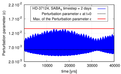
Figure 2: Variability of the perturbation parameter $\epsilon(t)$ for HD 37124 initial condition (Tab. 1). The initial condition has been integrated for 40 kyrs.

Table 2 displays estimates of the perturbation parameter $\epsilon$, which may be the measure of systems complexity in Tab. 1. The strength of mutual perturbations affects and forces a non-Keplerian evolution of the orbits, which we expect to be revealed in dynamical maps obtained with the fast indicators.

We determine this parameter for the nominal initial conditions as $\epsilon(t=0)$, see Tab. 2. Obviously, $\epsilon$ is a function of time, and, as illustrated for HD 37124 system (Fig. 2), it may vary during the orbital evolution. Therefore, we integrated all systems in Tab. 1 for $2\times 10^{3}$ outermost orbits, and we choose the maximal $\epsilon$ attained during the integration as the measure of the perturbation. We also note, that $\max\epsilon$ in Tab. 2 is only a reference value for dynamical maps, which span a range of orbital elements around the nominal parameters.

Table 2: Planetary systems classified by the perturbation parameter $\epsilon\equiv\|{\cal R}/{\cal H_{0}}\|$. Units are scaled with the choice of the Gaussian constant $k^{2}=1$. We consider coplanar systems, hence the number of the degrees of freedom for each system is $4\times N$, where $N$ is the number of planets.

system	$\|{\cal H}_{0}\|$	$\|\cal R\|$	$\epsilon(t=0)$	$\epsilon\equiv\max\epsilon$
HD 37124 b,c,d	$6\times 10^{-11}$	$4\times 10^{-13}$	$6\times 10^{-3}$	$1.3\times 10^{-2}$
Kepler-26 b,c	$9\times 10^{-12}$	$2\times 10^{-15}$	$2\times 10^{-4}$	$2.5\times 10^{-4}$
Kepler-60 b,c	$2\times 10^{-11}$	$3\times 10^{-15}$	$1\times 10^{-4}$	$1.6\times 10^{-4}$
Kepler-36 b,c	$1\times 10^{-11}$	$2\times 10^{-15}$	$2\times 10^{-4}$	$1.3\times 10^{-4}$
Kepler-29 b,c	$5\times 10^{-12}$	$3\times 10^{-16}$	$5\times 10^{-5}$	$5.3\times 10^{-5}$

We briefly characterize the sample of planetary systems below.

3.4.1 HD 37124: three planets in Jovian mass range

The HD 37124 planetary system (Vogt et al., 2005) is likely a compact configuration of three massive, Jovian-like planets discovered with the Radial Velocity technique. Its dynamics has been intensively investigated (Goździewski et al., 2008; Baluev, 2008; Wright et al., 2011). The perturbation parameter $\epsilon$ depends not only on the number of planets, but also on their mutual distance and their masses. Since we intend to use reversible SI with constant step size, even moderate eccentricities of compact orbits may be challenging for such numerical schemes, in the sense of accuracy and conservation of the integrals of motion. HD 37124 planetary system may be a good example of such demanding system. Its Jovian companions are present in a region spanned by low-order 2-body and 3-body MMRs (Goździewski et al., 2008; Baluev, 2008). Given their relatively large masses, the expected mutual gravitational interactions between the planets are the strongest in the sample, as shown in Tab. 2.

3.4.2 Kepler-26: two planets near 7:5 MMR

A resonant planetary system that exhibits complex dynamics is Kepler-26 (Steffen et al., 2012). It consist of two super-Earth planets near to the second order 7:5 MMR. Since the orbits may appear very near one to another, the mutual gravitational interaction may become also very strong. Kepler-26 has the largest $\epsilon$ value among Kepler systems displayed in Table 2. We note that actually Kepler-26 hosts four confirmed planets (Jontof-Hutter et al., 2016) but we neglect the innermost and the outermost planet since the available observations do not make it possible to reliably constrain their orbits and physical properties. The two-planet configuration is selected merely to have an example of a particular resonant system. This is motivated through the recent studies of this system (Jontof-Hutter et al., 2016; Hadden & Lithwick, 2016; Deck & Agol, 2016). We determined the planetary masses through a re-analysis of the long cadence Q1-Q17 TTV dataset in (Rowe et al., 2015).

3.4.3 Kepler-60: three super-Earths in the Laplace resonance

Recently, Goździewski et al. (2016) analysed the Kepler-60 extrasolar system and two resonant best-fitting solutions to the long cadence TTV measurements were found. Both of them may be interpreted as generalized, zeroth-order three-body mean motion Laplace resonance. The Kepler-60 is an example of an extremely compact configuration of relatively massive planets in orbits with periods of $\simeq 7.1$, $\simeq 8.9$ and $\simeq 11.9$ days, respectively. This resonance could be either a “pure” three-body MMR with only the Laplace critical argument $\phi_{L}=\lambda_{b}-2\lambda_{c}+\lambda_{d}$ librating with a small amplitude, or it may simultaneously form a chain of two-body 5:4 and 4:3 MMRs. In both cases the resonant Kepler-60 system is dynamically active and exhibits complex dynamics, both regarding limited zones of stable motions in the phase-space, as well as the presence of Arnold web structures. Given the close orbits, it is also a very demanding orbital configuration for tracking the long-term evolution and stability.

3.4.4 Kepler-36: massive super-Earths in stable chaos?

The Kepler-36 system is one of the first configurations detected with the analysis of its clear TTV signal (Deck et al., 2012). It exhibits the smallest $\epsilon$ in the sample shown in Tab. 2. This system brought our attention due to the presence of the so called stable chaos (Deck et al., 2012). The stable chaos means the long-term stable orbits in the sense of Lagrange, in spite of large mLCE. To verify this phenomenon with more recent TTV data, we did a preliminary re-analysis of the Q1-Q17 TTV measurements with the genetic algorithm (Charbonneau, 1995). We choose one of the best-fitting orbital solutions displayed in Tab. 1 for numerical tests of REM.

3.4.5 Kepler-29: two super-Earths in 9:7 MMR

We re-analysed the TTV measurements of the Kepler-29 system discovered in (Fabrycky et al., 2012) in our recent paper (Migaszewski et al., 2017). This compact configuration of two massive super-Earth planets in $\sim 5$ Earth mass range is separated at conjunctions by only $\simeq 0.01$ au. We found that the planets are in 9:7 MMR.

For the analysis here we used osculating elements in Tab. 1 for two dynamical models of the system. The first $N$-body model accounts for the mutual interactions of the planets. The Kepler-29 configuration has been also tested in the framework of the RTBP with two different splitting schemes of the Hamiltonian. We transformed the observational system to the RTBP model by fixing the inner mass to zero and the outer planet eccentricity also to zero. (In fact, this eccentricity may be very small, $e_{{\mbox{\scriptsize c}}}\simeq 0.001$ in the real configuration). This example is used as a transition model between low-dimensional dynamical system and the full $N$-body formulation.

4 Results and interpretation

In this Section we describe the results of testing the chaotic indicators defined in Sect. 2, when applied to the systems defined in Sect. 3, and characterized in Tabs 1 and 2.

Those configurations are non-integrable multi-dimensional conservative systems exhibiting resonant structures. We aim to illustrate these structures using two-dimensional dynamical maps (grids) composed of two canonical variables selected in a given initial condition. Usually, we choose the semi-major axis – eccentricity, $(a,e)$-plane for a selected planet, since these elements are rescaled canonical actions of the planetary Hamiltonian, Eq. 18-19. We vary these parameters along the axes of the grid within certain ranges, and the dynamical signatures of phase trajectories are then computed in each point of the grid. The results are colour-coded and marked in two-dimensional maps.

Fast indicators, like FLI and MEGNO, are designed to detect chaotic orbits for typically $10^{3}$–$10^{4}$ characteristic periods (Cincotta & Giordano, 2016), associated with the fundamental (proper) frequencies. However, in multi-dimensional dynamical systems, like planetary systems, the frequencies may span a range of a few orders of magnitude, like the mean motions (fast frequencies) and precessions of nodes and pericentres (secular frequencies) see, for instance (Malhotra, 1998). When these frequencies interact, various resonances emerge, like the two-body and three-body mean-motion resonances, secular resonances between precessional frequencies, and secondary resonances, which appear inside the MMRs (Morbidelli, 2002). Therefore the “fast indicator” feature, meaning a detection of chaotic behaviour for a relatively short interval of time, must be related to the local instability time-scale. The absolute integration interval required to reveal chaotic motions has always a particular dynamical context. In this paper we usually refer to typical time-scale of two-body MMRs expressed in units of the outermost planets’ period. It is not necessarily the same, as the time-scale of secular or secondary resonances, which is usually much longer.

In our experiments, we aim to reliably characterise the MMRs structures that may involve secondary resonances, as shown and justified below. Therefore we considered time-scales covering as many as $10^{5}$–$10^{6}$ outermost orbits. We also computed high-resolution scans, up to $1024\times 1024$ points, to avoid missing fine structures of the phase-space. Such time-scales and map resolutions may be redundant for routine computations. Yet they may cause a huge, non-realistic CPU overhead, depending on the particular algorithms.

For all numerical experiments, we used our multi-CPU, “embarrassingly parallel” farm code $\mu$Farm (Goździewski, in preparation) armed with a number of different fast indicators, which makes use of the Message Passing Interface (MPI) and GCC ver. 4.8. Intensive computations have been performed on Intel Xeon CPU (E5-2697, 2.60GHz) of the Eagle cluster at the Poznań Supercomputing and Networking Center. We refer to this particular CPU quoting code execution timings, and they should be used comparatively.

Finally, we do not intend to analyse the dynamical systems in detail. We focus on the sensitivity of the fast indicators for fine structures in the phase-space, associated with complex borders of chaotic and regular motions, the presence of separatrices and secondary resonances. We stress that this paper has an experimental character, regarding applications to the $N$-body dynamics. We test the REM reliability and sensitivity through investigating various computing schemes, in order to find the optimal one.

4.1 System 1: FGL Hamiltonian system

The Hamiltonian defined by Eq. 9 and the corresponding symplectic map version were studied for resonances and chaotic diffusion phenomena (Froeschlé et al., 2000; Lega et al., 2003; Froeschlé et al., 2005), with the help of fast indicators FLI and MEGNO (Słonina et al., 2015). The REM algorithm has been already tested for this Hamiltonian system by Faranda et al. (2012) with the canonical map technique for a relatively small time-span of $10^{3}$ iterations.

To preserve a homogeneous computing environment, we computed the REM maps with the symplectic SABA₃ scheme. For MEGNO, we used the symplectic tangent map (Mikkola & Innanen, 1999), in accord with Eq. 7. Also SABA₃ scheme has been used. Dynamical maps are shown in the $(I_{1},I_{2})$-plane, and show a small portion of the Arnold web for $\epsilon=0.01$. This value is significantly smaller from $\epsilon=0.04$ which was found as the borderline value for the global overlap of resonances, i.e., between Nekhoroshev and Chirikov regimes of the dynamics in this system (Froeschlé et al., 2000).

We scanned a small fragment of the phase-space in the $(I_{1},I_{2})$-plane with symplectic MEGNO for $T=10^{3}$ (upper panel of Fig. 3) and $T=10^{4}$ (bottom panel of Fig. 3) time units, respectively. Given a small value of the perturbation parameter $\epsilon=0.01$, it is clear that the $10^{3}$ periods integration interval is too short to reveal chaotic motions that appear due to high-order resonances. Apparently, $10^{4}$ time units is sufficient to detect main resonance structures. However, a complex chaotic zone due to resonances overlap, which is seen at the right edge of the MEGNO scans in Fig. 3, continuously develops for $10^{5}$ and $10^{6}$ periods (Fig. 4). We also note that in order to investigate the global diffusion, motion intervals as long as $10^{8}$ and $10^{9}$ characteristic periods must be considered, see (Lega et al., 2003, their Fig. 2) or (Słonina et al., 2015).

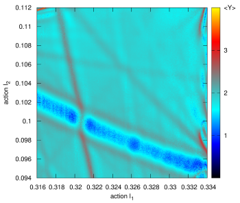
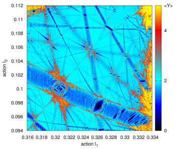
Figure 3: MEGNO in a $1024\times 1024$ grid of initial conditions in the $(I_{1},I_{2})$-plane of actions for the FGL Hamiltonian. Perturbation parameter $\epsilon=0.01$. The integrations were performed with the third-order SABA₃-scheme, time-step of $h=0.29$, for $10^{3}$ (upper plot) and $10^{4}$ (bottom plot) characteristic periods (time units), respectively. Integrations of MEGNO were interrupted if $\langle Y\rangle{}>10$. The time-step provides the relative energy conservation to $\sim 10^{-10}$.

Therefore, we extended the integration time to $T=10^{5}$, $10^{6}$ and $10^{7}$ characteristic periods, respectively. The results of the integrations for $10^{6}$ time units are illustrated in Fig. 4 and they perfectly agree for both methods. Periodic (black), resonant (blue/dark blue or grey) and chaotic (yellow/red or light grey) orbits are present in both maps corresponding closely. We notice subtle resonant structures between sharp (yellow/light grey) separatrices which are differentiated even better from neighbouring trajectories in the REM map.

For $T=10^{7}$ periods (not shown here), REM attains values as large as $10^{3}$ for chaotic orbits, and $10^{-4}$, for regular orbits. Nevertheless, only the overall variability range is essential to detect all fine structures of the phase-space, and we also found a perfect agreement of the derived REM scan with the MEGNO map.

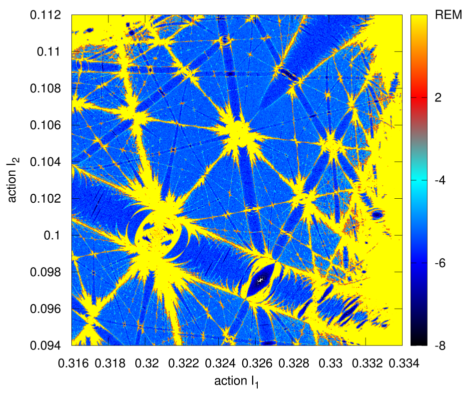
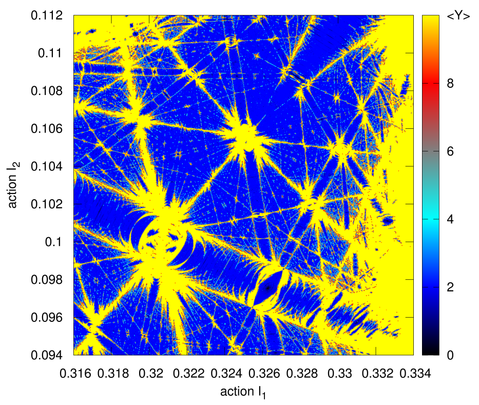
Figure 4: A comparison of REM (top panel, note the logarithmic scale) and MEGNO (bottom panel, symplectic tangent map algorithm) for the FLG Hamiltonian. The map is computed in a $1024\times 1024$ grid of initial conditions in the $(I_{1},I_{2})$-plane of actions. Perturbation parameter $\epsilon=0.01$. The integrations were performed with the third-order SABA₃-scheme, time-step of $h=0.29$ and for $10^{6}$ time units. Integrations of MEGNO were interrupted if $\langle Y\rangle{}>10$. This time-step provides the relative energy conservation to $\sim 10^{-10}$. The CPU overhead for single initial condition is $\sim 1$ second for REM, and between $0.1$ and $\sim 3$ seconds for MEGNO.

We note that some weak structures e.g., around $(I_{1}=0.327,I_{2}=0.107)$, may be missing in the MEGNO map for $T=10^{6}$ (Fig. 4) due to non-optimal choice of the initial variations ${\boldsymbol{\eta}}$ required to solve the deviation $\delta(t)\equiv\|{\boldsymbol{\eta}}\|$. To avoid systematic effects, we usually choose it randomly, following Cincotta et al. (2003). However, better strategies could be applied (Barrio et al., 2009), for instance, by selecting the initial ${\boldsymbol{\eta}}$ as the unit vector parallel to $\nabla{\cal H}$. On the other hand, the REM map for $T=10^{4}$ does not develop details seen in the MEGNO scan for the same integration interval, which in this particular case may be explained by longer saturation time-scale for REM than for MEGNO. This effect is illustrated in two panels of Fig. 3 for MEGNO. For stronger perturbation $\epsilon=0.04$, or larger $(I_{1},I_{2})$-range, spanning lower-order resonances, the equivalence of both algorithms is very close also for $T=10^{3}$–$10^{4}$, see, for instance (Faranda et al., 2012).

The CPU overhead for one initial condition is very different for both algorithms. For regular trajectories it is two times smaller for REM than for MEGNO. For chaotic and strongly chaotic trajectories, the MEGNO CPU overhead may be as small as $\sim 10\%$ of constant CPU overhead for REM, given the chaotic signature of chaotic orbits may be examined “on-line”, by tracking whether the current value of $\langle Y\rangle<{\langle Y\rangle}_{{\mbox{\scriptsize lim}}}$, where ${\langle Y\rangle}_{{\mbox{\scriptsize lim}}}\gg 2$. The total integration time is similar, however the REM implementation could be considered next to trivial.

4.2 System 2: HD 37124, three sub-Jupiter system

Here we use the initial condition for HD 37124 system in (Goździewski et al., 2008), which leads to dynamical structures in the semi-major axes plane closely resembling the Arnold web in the model Hamiltonian, Eq. 9.

Figure 5 shows such a map in the $(a_{{\mbox{\scriptsize c}}},a_{{\mbox{\scriptsize d}}})$-plane. The grid resolution is $640\times 640$ initial conditions, the integration time is 50 kyrs. The REM has been integrated with the SABA₃-scheme with the time-step of 5 days, while for the Bulirsch-Stoer-Gragg ODEX integrator, the relative and absolute accuracy has been set to $10^{-14}$. In this example, we used this general purpose ODE solver as a reference, to obtain a reliable dynamical map. Strong gravitational interaction between massive planets are expected, and the tested configuration resides in collisional, very chaotic zone.

Both dynamical maps agree very well, and all dynamical features may be found. We note however, that this is rather a borderline case of REM application, due to strongly chaotic regime. Also, due to fast linear growth of MEGNO for chaotic orbits in this zone, unstable motions are quickly revealed. Hence the integration time may be greatly reduced when some prescribed limit is reached. This is not the case for REM, because, usually, the whole integration must be performed before its value could be determined. However, the algorithm provides reliable results even in such a difficult case.

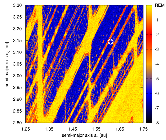
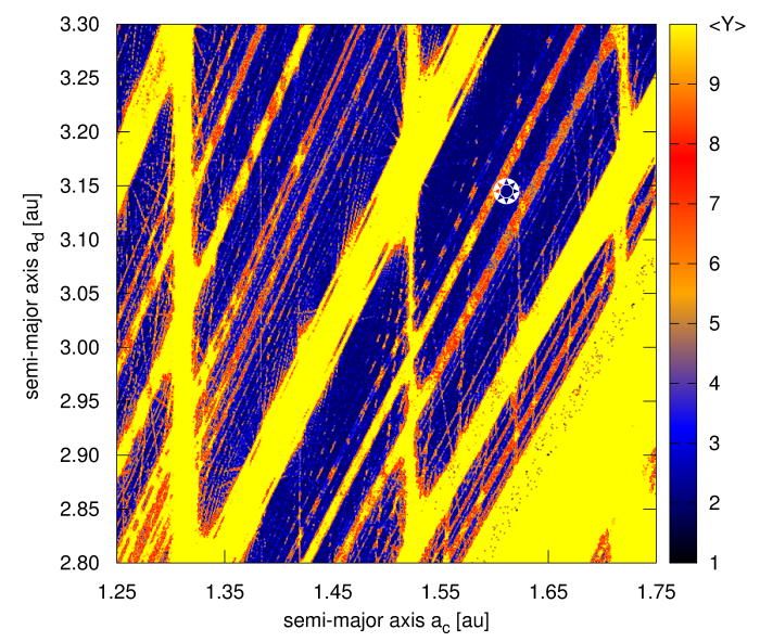
Figure 5: REM (top panel, note the logarithmic scale) and MEGNO (bottom panel) maps for the HD 37124 system presented in $(a_{{\mbox{\scriptsize c}}},a_{{\mbox{\scriptsize d}}})$-plane. SABA₃ REM algorithm with time-step of 5 days and forward integration time of 50 kyrs took $\sim 30$ seconds per initial condition. The CPU overhead for MEGNO varied between $\sim 1$ to $\sim 22$ seconds, given limiting $\langle{}Y{}\rangle=10$. The star symbol marks the nominal initial condition displayed in Tab. 1. The resolution is $640\times 640$ pixels.

4.3 System 3: Kepler-26 planetary system near 7:5 MMR

The orbital period ratios of the inner pair of super-Earth in the Kepler-26 system are close to the second order 7:5 MMR. Dynamical maps in the $(a_{{\mbox{\scriptsize b}}},e_{{\mbox{\scriptsize b}}}$)-plane shown in Fig. 6 illustrate a complex shape of the resonance. Both REM and MEGNO unveil its peculiar separatrix structure in its interior part, which exhibits a few disconnected stable regions.

We applied the most CPU efficient implementation of REM, which is the second order leapfrog-UVC(5) algorithm (Sec. 5). It is the mixed-variable scheme with Keplerian drift in universal variables without Stumpff series (Wisdom & Hernandez, 2015) and symplectic correctors (Wisdom, 2006) of the 5th order. For computing the MEGNO map, we used the tangent map algorithm and the SABA₄ integrator.

In the first experiment, the forward integration time of 16 kyrs was the same for both algorithms. We recall that REM requires effectively 32 kyrs integration, i.e., $5\times 10^{5}$ outermost orbits. Then the overall structure of the 7:5 MMR and higher order MMRs are the same in both maps. The algorithms reveal subtle stepping structure of chaotic configurations (around $0.0855~{}\mbox{au}$ and eccentricity around $e_{{\mbox{\scriptsize c}}}\sim 0.12$) as well as tiny islands of stable motion at the top of both maps. However, the elliptic shape of strong chaos surrounding weaker chaotic motions present in the MEGNO map, marked with a white arrow, are missing in the REM map. We attribute such fine structures to the presence of secondary resonances (Morbidelli, 2002) within the MMR zones.

We selected a few initial conditions in the arc structure, and the MEGNO was computed for these configurations to shed more light on their nature. The results are illustrated in Fig. 7. The chaotic orbits in this region appear as strictly regular up to $\sim 6\times 10^{4}$ outermost periods, given the MEGNO converged to 2 (the left panel in Fig. 7). However, for a longer integration interval the MEGNO diverges slowly. This experiment shows that we would miss the chaotic arc structure if the integration was restricted to the usual interval of $10^{4}$ outermost orbital periods, and extending the integration time to $\sim 10^{5}$ outermost orbits is unavoidable. We extended the integration time even more, as the safety factor.

In the arc region, the chaos may be called as slow in contrast to of the other parts of the map, in which the MEGNO indicates chaotic orbits for $\sim 10$–$100$ times shorter interval (hard chaos). In such a case, the “purely” numerical error growth does not make it possible to detect weakly chaotic orbits by the REM algorithm. Therefore we used the leapfrog-UV_γ variant (see Sect. 5.1) that relies in perturbing the initial condition vector, ${\boldsymbol{x}}_{0}={\boldsymbol{x}}_{T}+\gamma{\boldsymbol{\eta}}$, ($\gamma=10^{-14}$) at the end of the first interval of integration $(t=T)$. This simple modification brings a dramatic improvement of the REM sensitivity for chaotic motions. The results illustrated in the bottom panel of Fig. 6 are fully consistent with the MEGNO map in the middle panel. We also note that the total integration interval for REM of $2T=5$ kyrs is similar to the minimal integration time required to reveal the weakly chaotic orbits with MEGNO, see Fig. 7. In that case the CPU overhead of $\sim 8$ s is constant for REM, and varies between $\sim 1$–16 seconds for MEGNO integrated for 5 kyrs (strongly chaotic and regular orbits, respectively).

Furthermore, the REM map involves a signature of the collision zone of orbits defined geometrically as the solution of $a_{{\mbox{\scriptsize b}}}(1+a_{{\mbox{\scriptsize b}}})=a_{{\mbox{\scriptsize c}}}(1-a_{{\mbox{\scriptsize c}}})$. A dynamical border of this zone is marked as a change of shades across the REM map, around $e_{{\mbox{\scriptsize b}}}\simeq 0.14$. This zone appears below the collision curve determined by the semi-major axis $(a_{{\mbox{\scriptsize c}}}-R_{{\mbox{\scriptsize H}}})$, where $R_{{\mbox{\scriptsize H}}}$ is the mutual Hill radius for circular orbits

$$R_{{\mbox{\scriptsize H}}}=\sqrt[3]{\frac{m_{{\mbox{\scriptsize b}}}+m_{{\mbox{\scriptsize c}}}}{3M_{\star}}}\,\frac{a_{{\mbox{\scriptsize b}}}+a_{{\mbox{\scriptsize c}}}}{2},$$

and $m_{{\mbox{\scriptsize b,c}}}$, $a_{{\mbox{\scriptsize b,c}}}$ are the masses and semi-major axes of the planets, $M_{\star}$ is the stellar mass. The borderline is marked with thin, grey curve in the dynamical maps. This feature illustrates that the leapfrog implementations used in our experiments are robust for such near-collisional configurations, in spite of the step size that was kept constant across the whole grid.

We conclude that the REM detected all MMR’s structures and the overall shape of chaotic zones with relatively very small CPU overhead. This experiment brings a universal warning that if we are interested in a comprehensive characterisation of the fine structures of the MMRs, the time-scales of possible resonances must be examined with great care.

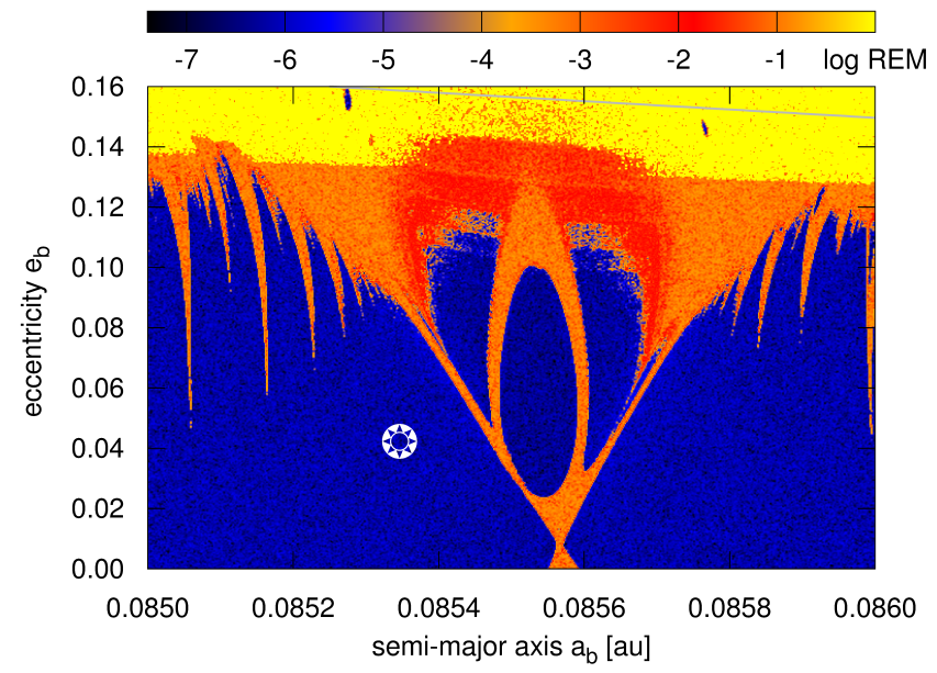
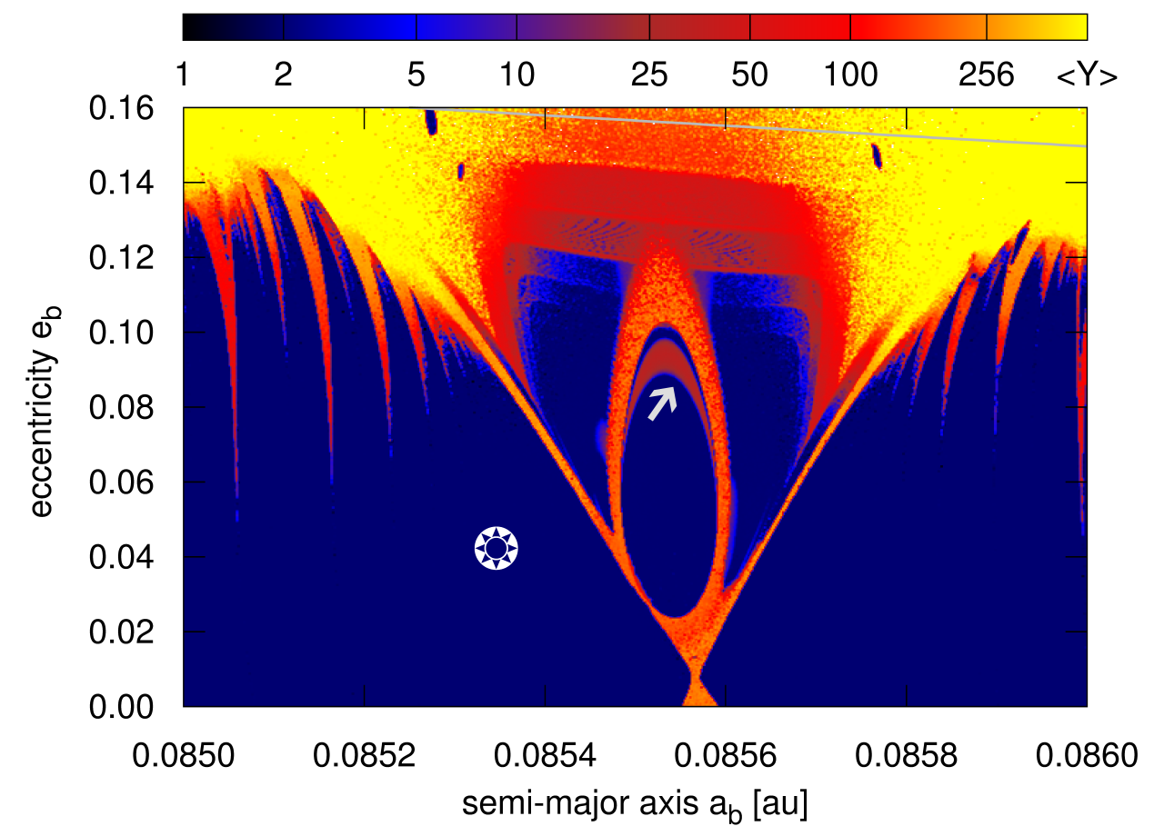
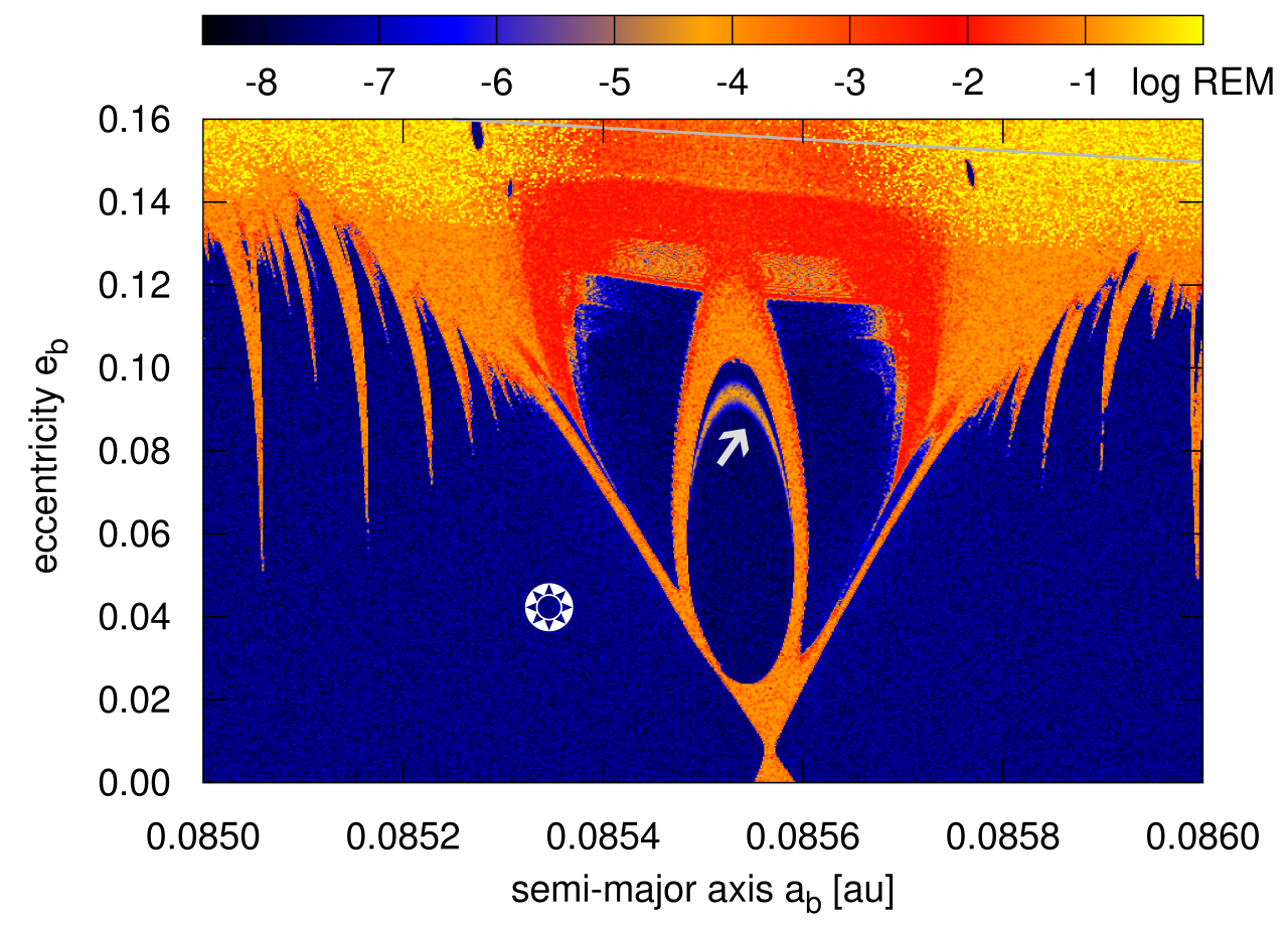
Figure 6: MEGNO and REM dynamical maps for Kepler-26. Top panel: the REM map in $(a_{{\mbox{\scriptsize b}}},e_{{\mbox{\scriptsize b}}})$-plane with the leapfrog-UVC(5) and time-step 0.25 days. The forward integration interval $16$ kyrs. Middle panel is for symplectic MEGNO map in the $(a_{{\mbox{\scriptsize b}}},e_{{\mbox{\scriptsize b}}})$-plane computed with SABA₄ scheme and time-step of $0.5$ days integrated for $16$ kyrs ($\sim 5\times 10^{5}$ outermost orbits). The maximum value of $\langle{}Y{}\rangle$ is equal to $256$. Bottom panel: the REM map computed with the leapfrog-UV_γ algorithm, $\gamma=10^{-14}$, time-step of 0.25 days and the forward integration interval of 5 kyrs ($\sim 1.5\times 10^{5}$ outermost orbits). White arrows show a structure of weakly chaotic solutions (it is absent in the top panel). The resolution of all maps is $800\times 600$ points. Thin grey curve in the top marks the mutual Hill radius separation of the orbits. The perturbation parameter $\max\epsilon$ vary across the map between $\sim 2.4\times 10^{3}$ and $\sim 3\times 10^{-3}$, see also Tab. 2. The star symbol marks the nominal initial condition displayed in Tab. 1. See the text for more details.

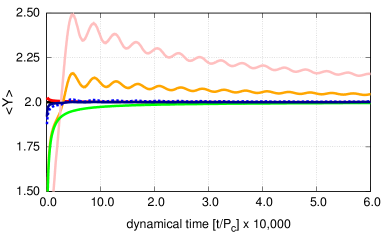
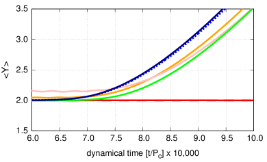
Figure 7: Temporal evolution of the MEGNO for a few initial conditions selected in the arc-like structure of weakly chaotic Kepler-26 configurations inside the 7:5 MMR, marked with arrows in the dynamical maps in Fig. 6 (middle and bottom panels). Time is expressed in units of the outermost period. The left panel illustrates apparently regular solutions for $\sim 6\times 10^{4}$ outermost orbits. However, after additional $\sim 2\times 10^{4}$ outermost periods and more (the right plot), the MEGNO indicates chaotic solutions in agreement with slow divergence. See the text for details.

4.4 System 4: the Laplace resonance in Kepler-60

The Kepler-60 system has been comprehensively analysed in (Goździewski et al., 2016), also regarding its dynamical structure. In Figure 8 we illustrate non-published MEGNO map (bottom panel) in the ($\varpi_{{\mbox{\scriptsize c}}},\varpi{{\mbox{\scriptsize d}}})$-plane that reveals a complex structure of the Laplace resonance around one of the best-fitting solutions (marked with a star symbol) to the TTV measurements in (Rowe et al., 2015), see Table 1. The top panel shows a high resolution REM map derived with the leapfrog-UVC(5) integrator for $18$ kyrs, with the time-step of $0.125$ d. With this time-step, the CPU overhead is huge, $\sim 80$ s per stable initial condition, i.e., still about two times smaller than the mean CPU time for MEGNO with the SABA₄ and the same time-step and forward integration interval. A significant fraction of the grid is spanned by strongly chaotic configurations, which are detected by MEGNO within a few seconds. This CPU time may be reduced with larger time-step, since our setup of this experiment is very conservative. We note that the long integration interval of $5\times 10^{5}$ outermost orbital periods has been selected in order to reveal potentially slow chaotic diffusion, as in the FGL example (see Figs. 3 and 4). The initial condition describing the Kepler-60 system in the zero-th order three-body Laplace resonance unveils qualitatively the same Arnold-web structures in the semi-major axes planes.

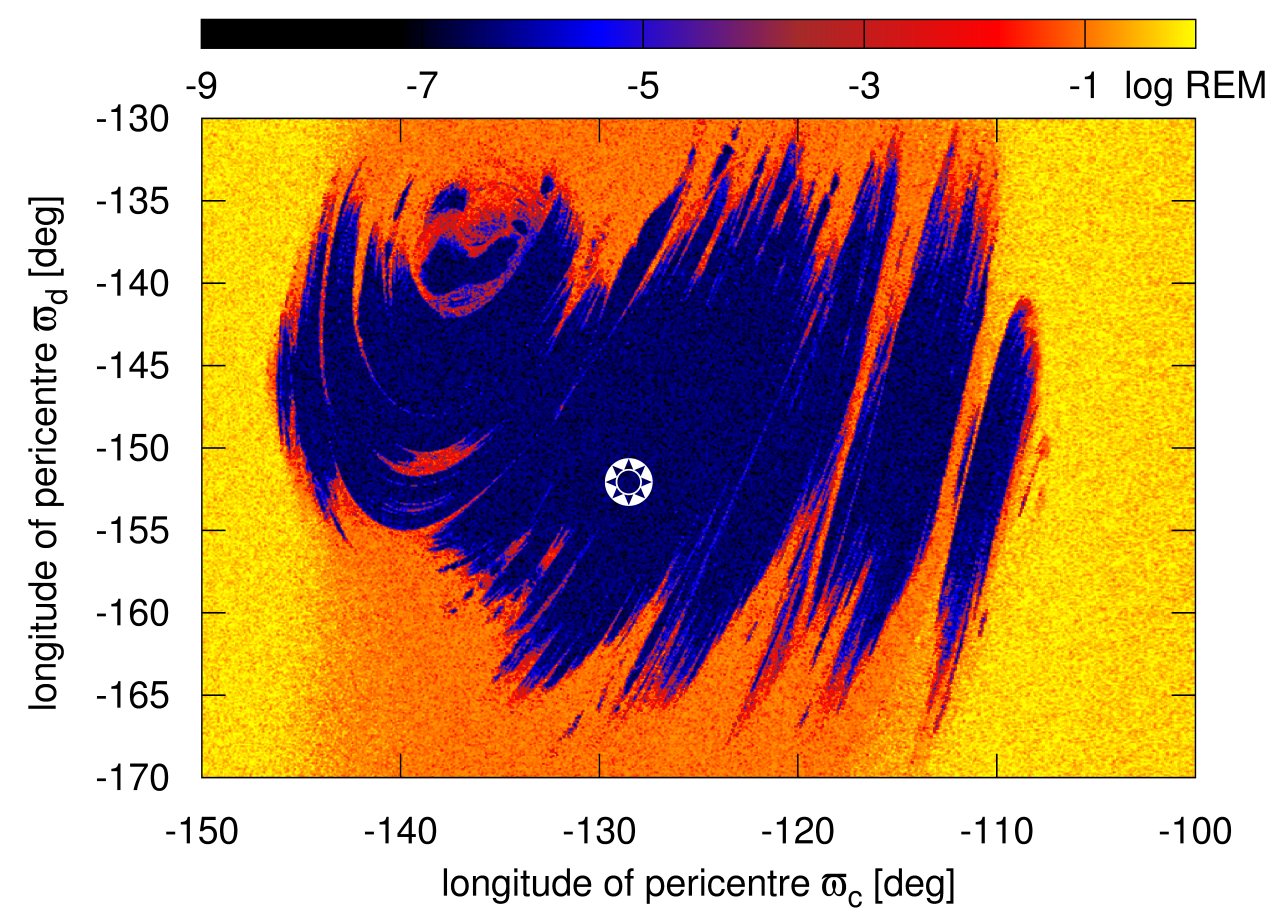
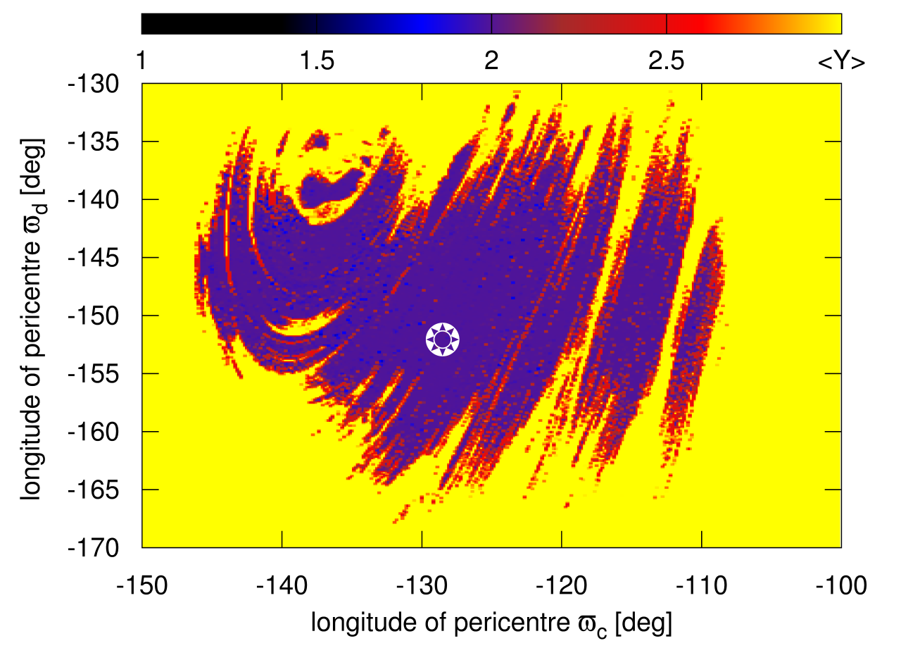
Figure 8: The REM (top panel) and MEGNO (bottom panel) dynamical maps for the Kepler-60 system in the $(\varpi_{{\mbox{\scriptsize c}}},\varpi{{\mbox{\scriptsize d}}})$-plane. The initial condition is displayed in Tab. 1 and marked here with the star symbol. Note that grid resolutions are different, $800\times 600$ for REM, and $720\times 720$ for MEGNO. Integration time is $16$ kyrs for MEGNO and forward integration interval of $16$ kyrs for REM.

4.5 System 5: Kepler-36 planetary system in 7:6 MMR

Dynamical maps in the $(a_{{\mbox{\scriptsize b}}},e_{{\mbox{\scriptsize b}}})$-plane for Kepler-36 (Deck et al., 2012), near to the first order 7:6 MMR are presented in Fig. 9. We integrated the MEGNO map (middle panel in Fig. 9) for 36 kyrs ($\sim 10^{6}$ outermost orbits) with the 4th order SABA₄ scheme and the tangent map algorithm (Goździewski et al., 2008) with the time-step 0.25 days. It looks like essentially the same as the map for 3 kyrs (bottom panel of Fig. 9) spanning $\sim 8\times 10^{4}$ outermost orbits. However, we note two fine unstable arcs marked with white arrows, which are not well “developed” for the shorter integration interval.

The leapfrog-UV(5) REM computed for the integration interval of 36 kyrs with time-step of $0.25$ days conserves the energy to $10^{-9}$ in relative scale. While the dynamical map (not shown here) reveals globally the same chaotic and regular solutions, two arcs marked with arrows in the MEGNO-panels in Fig. 9 are missing in the REM map. These features appear due to weakly chaotic solutions with longer instability time-scale than in the main part of the dynamical map, similar to the Kepler-26 model.

However, when the REM integration is done with the leapfrog-UV_γ scheme with time-step $0.25$ days and $\gamma=10^{-14}$, the weakly chaotic structures are present already for the forward integration time of 2 kyrs (only $\sim 5\times 10^{4}$ outermost orbits). Then the CPU overhead per initial condition is $\sim 3$ s, and between $1$ and $16$ seconds for MEGNO integrated for 3 kyrs. (We note that the weak, arrow-marked structures in Fig. 9 do not appear clearly for 2 kyr MEGNO integration). In the later case, the CPU overhead depends on the local value of mLCE, since we have set-up rather large limit of $\langle Y\rangle_{{\mbox{\scriptsize lim}}}=256$, which was used to classify initial condition as strongly chaotic.

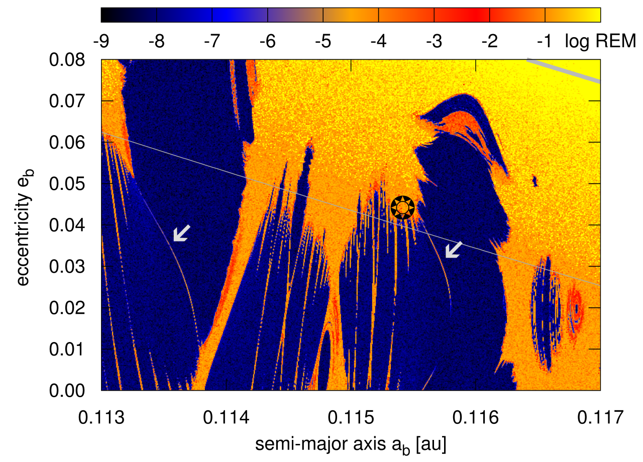
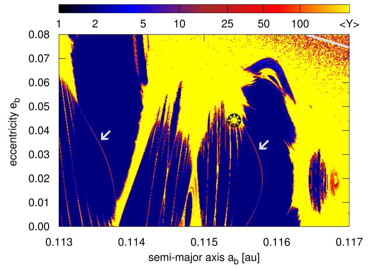
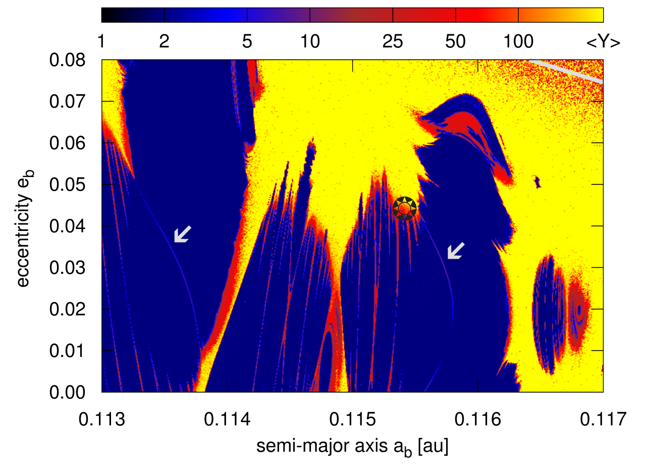
Figure 9: MEGNO and REM comparison for the Kepler-36 planetary system. Top panel is for the second order leapfrog-UV_γ REM map in $(a_{{\mbox{\scriptsize b}}},e_{{\mbox{\scriptsize b}}})$-plane, forward integration interval is 2 kyrs with CPU overhead of 3 s per initial condition and the magnitude of random perturbation is $\gamma=10^{-14}$. The CPU overhead is about of $4$ s. Middle and bottom panels are for the symplectic MEGNO with 4th order SABA₄ scheme, time-step $0.25$ days and the integration interval is 36 and 3 kyrs, respectively. For the bottom map, the CPU overhead is about $16$ s per stable orbit. The resolution is $800\times 600$. The star symbol marks the nominal initial condition displayed in Tab. 1. Thick light-grey curve in the upper-right corner marks the collision line of orbits. Thin light curve in the top panel is for the mutual Hill radius separation of the orbits.

Figure 9 shows a very good agreement between the maps of both indicators. The maps reveal a complex structure spanned by two MMRs, 6:5 MMR centred around $a_{{\mbox{\scriptsize b}}}\simeq 0.1135~{}\mbox{au}$, and 7:6 MMR centred around $a_{{\mbox{\scriptsize b}}}\simeq 0.1155~{}\mbox{au}$. From these two first order resonances an extended overlap zone emerges. We note a large range of REM values spanning 7 orders of magnitude. The border of the dynamical collision zone of the orbits may be clearly seen as a change of shades across the map, which is very close to a thick, grey curve determined by the mutual Hill radius separation from the geometrical collision curve (thick grey curve, Fig. 9). All major structures are fully recovered, in spite of the proximity to the collisional region.

This example shows that the REM algorithm modified with small perturbation of the initial conditions after the forward integration actually outperforms the MEGNO symplectic fourth-order SABA₄ scheme, providing the same sensitivity for chaotic orbits, with even smaller CPU cost for the REM dynamical maps.

4.6 System 6: stable chaos in 9:7 MMR of Kepler-29?

The Kepler-29 system has been found to be the most challenging example in our sample, and a demanding testbed for the fast indicator algorithms investigated in this paper.

In Fig. 10 we present the REM and MEGNO maps computed for $3\times 10^{4}$ outermost orbits, equivalent to $\sim 1.2$ kyrs interval which should be typically sufficient to reveal chaotic motions associated with the two-body mean motion resonances. The map in the upper panel of Fig. 10 has been obtained with the symplectic MEGNO algorithm with SABA₄ and a step size of $0.25$ days, respectively. The bottom left panel shows the REM dynamical map obtained with the leapfrog-UVC(5) scheme and for the same forward integration interval of 1.2 kyrs. Apparently, both maps agree perfectly. The overall shape of the 9:7 MMR is clearly recovered in both maps, and major structures are the same in the region of moderate eccentricities.

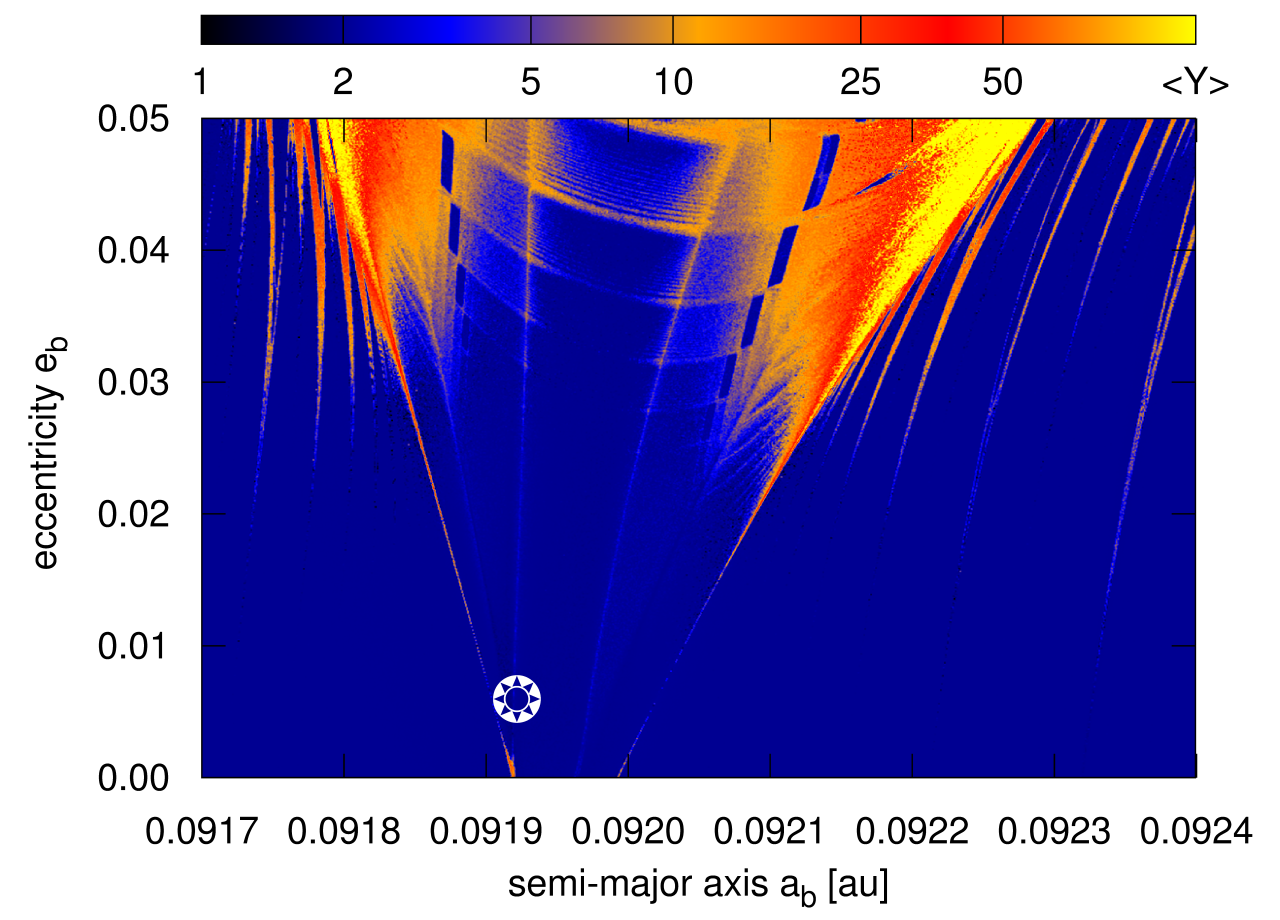
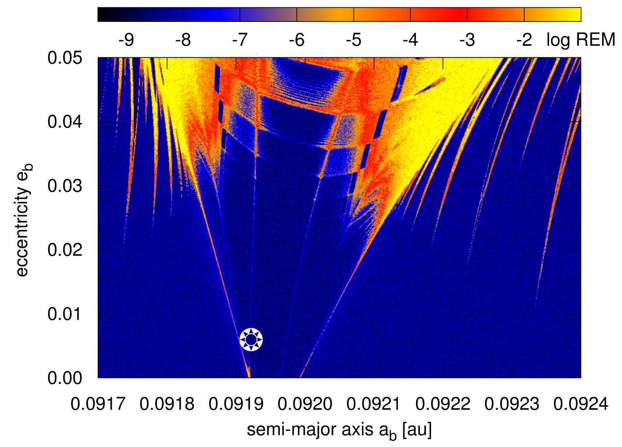
Figure 10: Dynamical maps for Kepler-29 in the $(a_{{\mbox{\scriptsize b}}},e_{{\mbox{\scriptsize b}}})$-plane. The upper panel is for symplectic MEGNO map with SABA₄ integrator, time-step of $0.5$ days, integrated for 1.2 kyrs ($3.3\times 10^{4}$ outermost periods). The bottom panel is for the REM map with the leapfrog-UVC(5) integrator, time-step of $0.25$ days, and the integration interval is $2\times 1.2$ kyrs. The resolution is $1024\times 768$ points. The star symbol marks the nominal initial condition displayed in Tab. 1.

However, keeping in mind that the MEGNO integration interval may be too short, as in the Kepler-26 example, we extended the integration interval up to $2\times 10^{6}$ orbits (72 kyrs). This experiment reveals a wide chaotic strip in the centre of the V-shaped MMR (top-left panel in Fig. 11). We note that mLCE in the central strip is as large as $\sim 0.02/\mbox{yr}^{-1}$, given that the maximal value of ${\langle Y\rangle}=768$ has been reached for 72 kyrs, and we approximate mLCE $\equiv\lambda=2{\langle Y\rangle}$, in accord with Eq. 7. Actually, we know a posteriori that the integration time to detect this structure with the help of MEGNO is $\simeq 3$ kyrs and it corresponds to $6\times 10^{4}$ outermost periods. Yet we show again that the usual “rule of thumb” choice of $10^{4}$ outermost periods for integrating MEGNO would be not sufficient, as we demonstrated in Fig. 7 for the Kepler-26 system.

Surprisingly, for the same long, total integration time of 72 kyrs, the REM with SABA₄ and leapfrog-UVC(5) integrators do not “see” the wide chaotic strip in the middle of the 9:7 MMR. Indeed, the top-right panel of Fig. 11 shows the REM map computed with the symplectic SABA₄ scheme. A thin, vertical grey line across this map marks the change of the time-step from $0.25$ days to $0.5$ days. The longer time-step has no impact on the results besides smaller REM (darker shade).

We confirmed the discrepancy with the third fast indicator, the FMFT. We choose the sampling time-step of $0.5$ days and $N=2^{22}$ for the same grid of initial conditions as for MEGNO and REM (Fig.11). This is equal to $T\sim 2\times 10^{5}$ outermost periods, hence one order of magnitude longer interval than usually required by MEGNO to reveal low-order two body MMRs. No signs of geometric instability have been found in the problematic zone, in the sense of a variation of the osculating elements and the proper mean motions (bottom-left panel in Fig. 11). Moreover, we found a very close agreement of the REM and FMFT signatures. These maps could be hardly distinguished one from the other.

The FMFT experiment reveals a very slow chaotic diffusion of the orbital elements, similar to the Kepler-29 and Kepler-36 cases, yet in much more extended zone. Therefore we applied the REM algorithm with the middle-interval perturbation. In this experiment we choose the middle-interval perturbation of the state vector as $\gamma=10^{-14}$, and we integrated the system with the leapfrog-UV_γ scheme (Sect. 5.1). The time-step of $0.25$ days and the forward integration interval is only 3 kyrs, i.e., the minimal integration time for MEGNO to reveal the instability. For this time interval, the dynamical REM map in the bottom-right panel of Fig. 11 fully corresponds to the MEGNO map integrate for 72 kyrs, and it reveals both all major and tiny structures of the 9:7 MMR. The CPU overhead is in this case only $\simeq 5$ seconds, which is roughly two time less than for SABA₄–MEGNO integrated for the same interval.

The FMFT experiment helps us to explain the different signatures of the indicators by the so called “stable chaos” phenomenon. This phenomenon was discovered by Milani & Nobili (1992); Milani et al. (1997) for asteroid motions. It is found to be due to high order MMRs with Jupiter in combination with secular perturbations on the perihelia of the asteroids. The amazingly complex structure of the 9:7 MMR in the Kepler-29 system is likely related to the secondary resonances which are characteristic for low-eccentricity systems and appear due to a commensurability of the resonant frequency with the apsidal libration frequency (e.g., Morbidelli, 2002). While a detailed analysis of the Kepler-29 system is beyond the scope of this paper, it may be a clear evidence of the stable chaos for the Kepler-29 planets in low-order 9:7 MMRs. This is unusual since large mLCE appear due to secular interactions of relatively low-dimensional, two planets system only. We found a similar effect, though much subtle, in the Kepler-26 system.

The results for Kepler-29 are the most clear indication of a possibility of a non-unique classification of particular unstable (chaotic) orbits by different fast indicators due to locally varied time-scales of instability. In the Kepler-systems, the slow chaotic diffusion of orbital elements clearly appears in the regions spanned by MMRs. Regarding the canonical REM algorithm, for these weakly chaotic solutions the numerical errors are too small to provide sufficient Lyapunov error and sufficiently distant shadow orbit. By enforcing this perturbation by adding an appropriate $\gamma{\boldsymbol{\eta}}$ term only once after the forward integration interval, we enhance the sensitivity of the algorithm for chaotic orbits. Given that the perturbation is very small (at the $10^{-14}$ level), both the REM signature for regular orbits and the energy conservation are not affected (see Sect. 5 for more details).

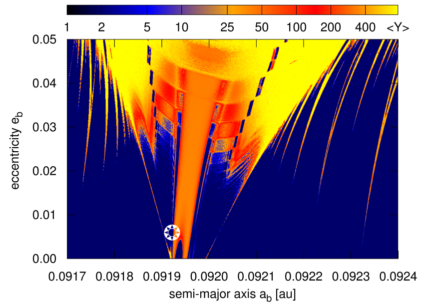
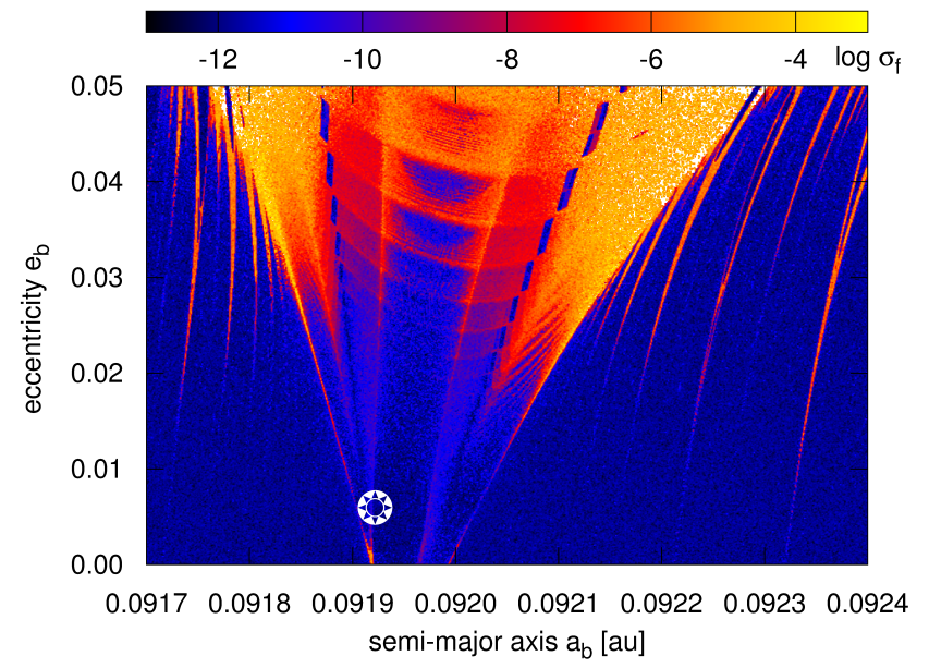
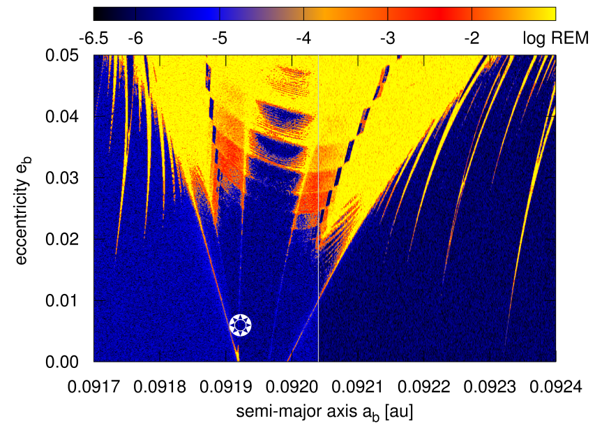
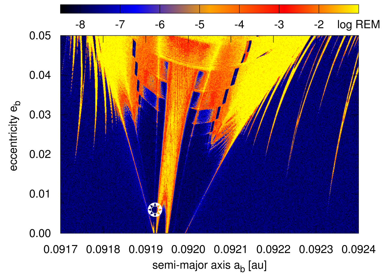
Figure 11: Dynamical maps for Kepler-29 in the $(a_{{\mbox{\scriptsize b}}},e_{{\mbox{\scriptsize b}}})$-plane. Top-left panel for symplectic MEGNO map with SABA₄ integrator, time-step $0.5$ days, integrated for 72 kyrs ($2\times 10^{6}$ outermost periods). Top-right panel is for the $N$-body REM map, divided in two parts: the left is for SABA₄ with time-step $h=0.25$ d, and the right one is for SABA₃ with time-step $h=0.5$ days, forward integration interval is 36 kyrs ($10^{6}$ outermost periods). Bottom-left panel is for the diffusion frequency of the mean motion of the inner planet, the total integration spans 6 kyrs, or $2\times 2^{22}$ time-steps of 0.5 day ($\sim 2\times 10^{5}$ outermost periods). Bottom-right panel is for the REM map with the leapfrog-UV_γ integrator, time-step 0.25 days, and the forward integration interval is 3 kyrs $\simeq 10^{5}$ outermost periods. The resolution of all grids is equal to $1024\times 768$ points. The star symbol marks the nominal initial condition displayed in Tab. 1.

4.7 System 7: Kepler-29 as the restricted three body problem

In the last experiment, we test a modified configuration of the Kepler-29 system (Tab. 1) as the RTBP configuration, which is close to the 9:7 MMR in the $N$-body model. We made this experiment to illustrate some differences that may appear when REM is computed with different splittings of the same Hamiltonian.

The results are illustrated in Fig. 12. A map in the top panel has been obtained in the framework of the $N$-body problem (Sect. 3) with the leapfrog-UVC(8) algorithm with step size of $0.25$ days and integration time of 3.6 kyrs. The middle panel shows the REM dynamical map obtained with the 4th order Yoshida integrator, and the forward integration interval of 3.6 kyrs ($10^{5}$ revolutions of the binary). However, due to the particular Hamiltonian splitting (Sect. 3.2), which is “blind” for the planetary character of the model investigated, the step size has to be as small as $0.0625$ d to conserve the energy at $\sim 10^{-8}$ level.

The overall shape of the 9:7 MMR is clearly recovered in both maps, and the major structures are the same. However, significant differences of the absolute REM values appear in the regions of the central, V-shaped MMR, as well as in higher-order MMRs shown as smaller “drops” out of the central structure. The background level of REM for stable orbits of $10^{-7}$–$10^{-6}$ can be the basis to identify regular orbits.

The RTBP map derived with the Yoshida scheme exhibits more clear differentiation of regular orbits. We attribute it to a combination of two numerical effects. One is the different sensitivity for stable-resonant and stable-quasiperiodic orbits (we recall the FGL Hamiltonian example). For the Yoshida integrator, there is also a numerical instability of the “drift” (Eq. 14), which effectively means the rotation by angle $2h$. It results in the energy drift (Petit, 1998). Indeed, we found that the Yoshida scheme exhibits such a strong, linear energy drift re-inforced by smaller step sizes. This numerical instability has likely a different impact on the REM index in stable resonant regions and in stable quasi-periodic zones. They are strongly discriminated as dark-blue (dark grey) and light-cyan (light-grey) regions in the bottom REM map in Fig. 12.

Yet the $N$-body variant of REM outperforms the RTBP model in the CPU overhead. A single initial condition was integrated with the leapfrog-UVC(5) scheme for $4.4$ seconds, while the 4th order Yoshida integrator required $\sim 7.7$ seconds, though the energy error is worse by 1-2 orders of magnitude.

For reference, we also computed the MEGNO map (the bottom panel in Fig. 12), with the ODEX integrator, for the same interval of 3.6 kyrs. For this integration time the separatrices of the 9:7 MMR, its fine structure as well as lower-order MMRs appear as much less clear than in the REM maps. We note that this result does not change when we use the SABA₄ integrator.

We conclude that the leapfrog-UVC(5) REM algorithm may be used for investigating the dynamical structure of 2-planet Kepler systems, if they could be described in the framework of RTBP. We also note that the RTBP could be easily generalized with perturbations like primaries oblateness, radiation, and other conservative effects. As long as such perturbed problems could be solved with symplectic and reversible algorithms, REM may be the method of choice, given its straightforward implementation and a great sensitivity for chaotic orbits.

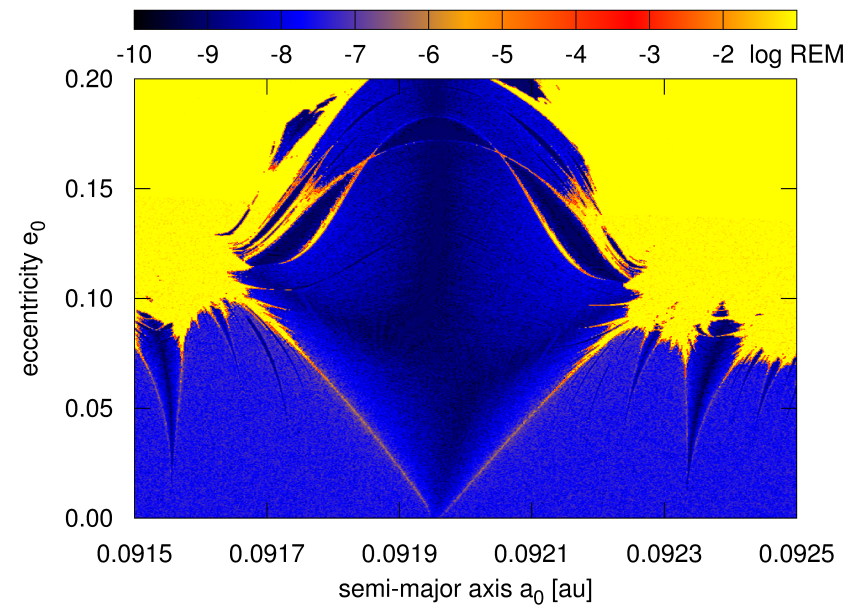
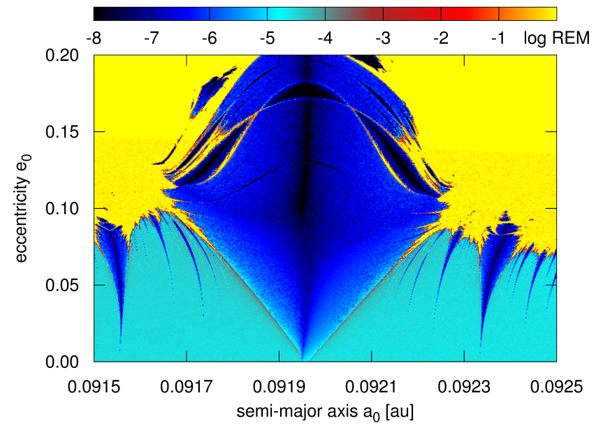
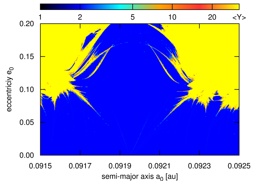
Figure 12: Dynamical REM maps for the $N$-body and RTBP models (Sect. 3.3 and 3.2) for the Kepler-29-like system in the $(a_{0},e_{0})$ plane of the mass-less planet (Tab. 2). The top panel is for the $N$-body REM map with leapfrog-UVC(8) scheme, step size 0.25 d, the middle panel for the REM map derived for the RTBP-Hamiltonian integrated with the 4th order Yoshida scheme and time-step of 0.06125 d, and the bottom panel is for the MEGNO map computed with the ODEX integrator, the relative and absolute accuracy set to $10^{-15}$. For the REM maps the forward integration interval is 3.6 kyrs ($\sim 10^{5}$ periods of the binary), which is the same as for the MEGNO map. The grid resolution is equal to $900\times 768$ points.

5 Numerical setup and CPU efficiency

The most important feature of integrators used to compute the dynamical maps in Sect. 4 is the time-reversibility, closely related to conservation of the first integrals (Hairer et al., 2006). Usually, as much as $10^{5}$–$10^{6}$ outermost orbital periods must be considered when we want to investigate large volumes or fine structures of the phase-space of the Kepler planetary systems. Therefore the CPU overhead is the next critical factor for choosing integration schemes. We focus on low-eccentric planetary systems, when constant time-step is permitted due to relatively small mutual perturbations. We aim to analyse the most relevant integrators features, like the maximal reliable time-step, total integration time and preservation of the first integrals of motion, when used to compute the dynamical maps in Sect. 4. We use the Kepler-26 and Kepler-36 systems as testbed configurations.

5.1 Keplerian solvers and the leapfrog implementations

The classic “planetary” leapfrog scheme (Hairer et al., 2006), and its derivatives, as the SABA_n/SBAB_n schemes (Laskar & Robutel, 2001) or Yoshida integrators (Yoshida, 1990), are composed of the Keplerian “drift”, which propagates the system along Keplerian orbits, and “a kick”, which corresponds to the linear advance of the momenta. This is the genuine Wisdom & Holman (1991) scheme, known as the mixed-variable symplectic leapfrog. A crucial factor for implementing this algorithm is an accurate and fast solver for propagating the initial conditions at Keplerian orbit. In our implementation, we used the Keplerian drift code of Levison & Duncan (1994) in their SWIFT package, which become a de-facto numerical standard. A version of the leapfrog and higher order schemes with the DL drift are postfixed with “-DL” throughout the text. We also used a new, improved Keplerian solver by Wisdom & Hernandez (2015), kindly provided by the authors (Jack Wisdom, private communication). This solver is based on the universal variables (Stumpff, 1959), but without Stumpff series. The REM variants with this solver are postfixed by “-UV”.

Furthermore, to improve the accuracy of the classical leapfrog integrations, we used symplectic correctors introduced by Wisdom (2006). Our most “sophisticated” leapfrog REM implementation is then the leapfrog-UVC($n$) algorithm with Wisdom correctors of order $n=1,3,5,7,8$.

Finally, we made extensive numerical experiments to improve the REM sensitivity to slow chaotic diffusion inside the MMRs in the Kepler-26, Kepler-36 and Kepler-29 systems. The sensitivity may be greatly enhanced by introducing a random and very small perturbation of the state vector (initial condition) ${\boldsymbol{x}}_{T}$ at the end of the forward integration interval ($t=T$). It becomes the initial condition ${\boldsymbol{x}}_{0}$ for the backward integration:

$${\boldsymbol{x}}_{0}\equiv{\boldsymbol{x}}_{T}+\gamma{\boldsymbol{\eta}},$$

where, in accord with Eq. 30, $\gamma$ is the magnitude of the perturbation, and ${\boldsymbol{\eta}}$ is the unit vector with random components. Here, we choose $\gamma\sim 10^{-14}$, which provides the energy conserved well bellow the limit introduced by the integrator scheme itself. This step may be considered as simulating the error growth after much longer integration interval, or by selecting a shadow orbit nearby the tested solution. We call this variant of the REM as the leapfrog-UV_γ algorithm (UV_γ, i.e., the leapfrog with the Keplerian drift in universal variables and the $\gamma$-perturbation added at the end of the first interval of integration).

5.2 Time-reversibility and CPU overhead of SABA_n schemes

Without the round-off errors, a symmetric integrator would be time-reversible independently of the constant step size (Hairer et al., 2006). When the round-off errors are present, the algorithm introduces certain systematic errors depending on the number of steps. Therefore the REM final values may subtly depend on the time-step, Hamiltonian splitting, and total integration time.

Fig. 13 illustrates numerical single-step reversibility for the second order and the 10th-order SABA_n schemes as well as the leapfrogs with DL and UV solvers. In this test, we perform one forward integration time-step $h$ and then the backward one for $-h$. Clearly all schemes are time-reversible up to machine-precision (IEEE floating-point arithmetic, MACH$~{}\sim 2.2\times 10^{-16}$), as expected, for a wide range of time-steps. In fact, the reversibility is even better than the MACH value, since the calculations were performed on INTEL-architecture CPU with registers of 80 bits.

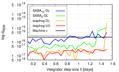
Figure 13: Time-reversibility test of SABA_n and the leapfrog schemes, postfixed with DL and UV, which stand for the Keplerian drift implemented in the (Levison & Duncan, 1994) and (Wisdom & Hernandez, 2015) Keplerian solvers, respectively. The time-reversibility breaks when the time-step is too large.

For a longer forward time interval, equal to $800$ yrs and large number of steps, the final REM value for a stable orbit slowly increases with total number of time-steps (Fig. 14), essentially uniformly for different order methods and step sizes. For this relatively short integration time, REM is preserved to $~{}10^{-7}$.

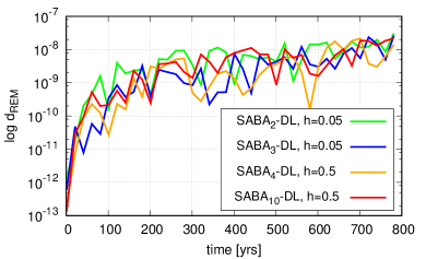
Figure 14: Time-reversibility test of SABA_n schemes for $800$ yrs. We choose a stable HD 37124 configuration to test. SABA₂ (green/black line), SABA₃ (blue/dark-grey line) final REM values are illustrated for the time-step $h=0.05$ days, and SABA₄ (orange/grey line) and SABA₁₀ (red/light-grey line) for $h=0.5$ days. Depending on selected scheme, the energy is preserved with a different precision but for all integrator schemes the relative error does not exceed $10^{-9}$ in the relative scale.

Fig. 15 presents the relative CPU overheads for SABA_n schemes for the REM integrations of a stable orbit in the Kepler-26 system. The time-step was changed between $0.1$ and $1$ days. The forward integration time is fixed to $10$ kyrs. For short time-steps $\sim 0.1$ days, which correspond to $1/170$ of the outermost orbital period ($\sim 17.25$ days), the CPU time would be essentially non-realistic and unacceptable for massive integrations with high-order methods, like SABA₆ or SABA₁₀. For lower-order SABA_n integrators, the CPU overhead is still significant, and depends weakly on the Keplerian solvers. We observed some gain of accuracy and performance when using the UV-drift code. At the same time, the reversibility test in Fig. 16 suggests that the REM value depends a little on the integrator scheme used for a wide range of time-steps. This could mean that low-order SABA_n algorithms should be preferred for REM calculations to the higher order integrators, provided that a reasonable relative energy conservation of $10^{-7}$–$10^{-8}$ is guaranteed for regular orbits.

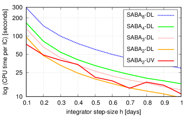
Figure 15: A relative CPU overhead for REM with different SABA_n schemes postfixed with -DL and -UV, which stand for the Keplerian drift implemented in the (Levison & Duncan, 1994) and (Wisdom & Hernandez, 2015) Keplerian solvers, respectively. The CPU time is expressed in seconds per single initial condition and total integration time of $2\times 10$ kyrs.

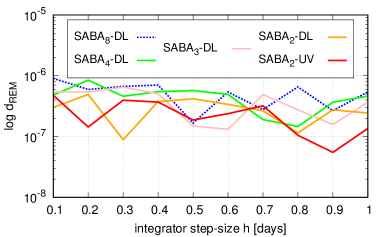
Figure 16: REM values for a range of time-steps and total integration time of $2\times 10$ kyrs. A stable configuration of the Kepler-26 planetary system (Tab.1) is tested. SABA_2,4,8 integrators are postfixed with -DL and -UV, which stand for the Keplerian drift implemented in the (Levison & Duncan, 1994) and (Wisdom & Hernandez, 2015) solvers, respectively.

5.3 SABA_n vs. the second order leapfrog

The results illustrated in Fig. 14 and close to uniform behaviour of REM inspired us to test the second order, classic leapfrog algorithm. Its CPU overheads may be greatly reduced by concatenating subsequent half-steps. For instance, the sequence drift-kick-drift, once initialized with half-step drift, may be continued by full time-steps drift-kick sequence, reducing the number of the force calls. The integration sequence is finalized with half-step drift, when the end-interval result of the integration is required. This is the REM case.

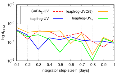
Figure 17: Reversibility test for different leapfrog schemes: leapfrog-UV with the UV drift (blue/dark-grey thin line), leapfrog-UV(8) with the UV solver and (Wisdom, 2006) correctors of the eight order (orange/grey thick line), and with the UV solver and $\gamma$ perturbation (leapfrog-UV_γ with $\gamma=10^{-14}$, green/light-grey curve). For a reference, SABA₂ scheme with the UV drift is illustrated (SABA₂-UV, dashed curve).

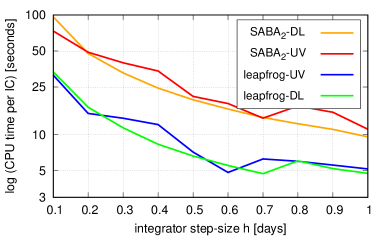
Figure 18: A comparison of REM CPU overhead for variants of the leapfrog: SABA₂ with the DL and UV drifts (orange/light grey and red/dashed light grey lines), and leapfrog with the DL and UV drifts (blue and green lines/thick grey lines). Total integration time is $2\times 10$ kyrs.

Figure 17 illustrates the REM outputs for a stable configuration in the Kepler-26 system, when integrated for the forward interval of $10$ kyrs and different variants of the leapfrog algorithm. The step size is varied between $0.1$ and $1$ days, though we warn the reader that $h>0.5$ day may introduce numerical instability for chaotic orbits. This test shows that all tested schemes, including the $\gamma$-perturbed variant of the leapfrog-UV_γ with $\gamma=10^{-14}$, provide similar REM outputs. We note that REM fluctuations spanning roughly $1$ order of magnitude do not have likely any systematic meaning, given a very small statistics of measurements.

However, quite surprising results are provided by the CPU time test illustrated in Fig. 18. Given the classic leapfrog variants optimized by the concatenation of sub-steps, these schemes systematically outperform SABA₂ almost by two-times, independent of the step size in a range of $[0.1,1]$ days. We found that uncorrected leapfrog fails the REM test for shorter time-steps than its corrected variant.

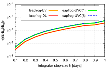
Figure 19: Mean error of the energy for the leapfrog variants tested in this paper. The Kepler-26 initial condition was examined (Tab. 1). Here, leapfrog-DF means the second order leapfrog with (Levison & Duncan, 1994) Keplerian drift, leapfrog-UV means the leapfrog with Keplerian drift code by (Wisdom & Hernandez, 2015), leapfrog-UVC($n$) is for this algorithm and (Wisdom, 2006) correctors of order 1 and 5, respectively.

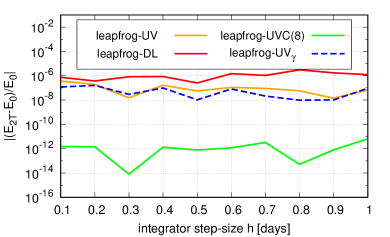
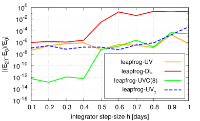
Figure 20: Energy error after integrating the REM value for the leapfrog variants tested in this paper (see captions of the previous figures), for Kepler-26 (top panel), and Kepler-29 (bottom panel) initial conditions, see Tab. 1. The magnitude of perturbation of the initial condition after the forward integration, $\gamma=10^{-14}$. See the text and captions of the previous figures for the meaning of labels.

For sufficiently small step sizes, the corrected leapfrog with Keplerian drift by Wisdom & Hernandez (2015) may be the less CPU demanding REM algorithm, still providing reliable results, as compared to MEGNO computed with high-order SABA integrators, or the non-symplectic Bulirsch-Stoer-Gragg scheme. To illustrate that, in Fig. 19 we computed the mean error of the energy for $10$ kyrs of the Kepler-26 system (Tab. 1). We used four variants of the second order leapfrogs. Even for step sizes as large as $1$ day, the mean error of energy is $\sim 10^{-6}$, and with some gain with the symplectic correctors.

Next Fig. 20 is for the energy error computed with the REM estimation, i.e., after the interval $t=2T\equiv T+\|-T\|$, relative to the initial value at $t=0$, where $T$ is the forward integration time. We tested two systems, Kepler-26 (top panel), and Kepler-29 (bottom panel). For this particular numerical setup, the Wisdom correctors improve the energy conservation by a few orders of magnitude, essentially for zero CPU cost. This certainly improves the REM estimate for regular orbits, by reducing the deviation introduced by the surrogate Hamiltonian solved by the leapfrog, from the true one. A small, middle-interval change of the initial condition in the $\gamma$-perturbed variant of the REM, based on the leapfrog-UV_γ scheme ($\gamma=10^{-14}$) does not introduce any impact on the energy conservation w.r.t. the unperturbed version. Moreover, the results for Kepler-29 bring a clear warning: too large step size may cause numerical instability of the Keplerian solvers, as well as diminish the great gain of accuracy provided by the correctors. In fact, our large-scale numerical tests in the previous section for Kepler-29 failed with step sizes longer than $0.5$ days.

Our experiments with Kepler systems in Tab. 1 show that step sizes of $\sim 1/40$ of the innermost orbital period provide the optimal conservation of the energy $\sim 10^{-8}$–$10^{-9}$ in the relative scale. However, a fine tuning of the step size may be required for systems of interest, given their proximity to collision and strongly chaotic regions of motion.

6 Conclusions

In this paper we propose an application of the fast indicator called REM, based on the time-reversibility of Hamiltonian ODEs, to a particular class of planetary systems. They are characterized by quasi-circular orbits and relatively small mutual perturbations. The REM algorithm has been introduced elsewhere. Our numerical application of REM for planetary systems presented in this paper can be regarded as an extension of the analytic theory for quasi-integrable non-linear symplectic maps.

Besides presenting the theoretical aspects, we show that REM is equivalent to variational algorithms, like mLCE, FLI and MEGNO, provided that dynamical systems of interest may be investigated with symplectic and symmetric numerical algorithms. Such systems span the FGL Hamiltonian exhibiting the Arnold web, the restricted three body problem and a few multiple systems discovered by the Kepler mission. The Kepler planetary systems are the main target of our analysis, since their eccentricities are damped by the planetary migration, and a low range of eccentricities is typical. Moreover, the Kepler systems are very compact, and are found in 2-body and 3-body MMRs, forming resonant chains. This leads to rich dynamical behaviours.

Revealing the phase-space structures of these dynamically complex systems is possible thanks to CPU efficient fast indicators. We found that REM may be such a useful numerical technique, particularly for investigating the short-term, resonant dynamics of the Kepler systems. Given its simple implementation, it provides essentially the same results, as much more complex algorithms based on variational equations or the frequency analysis.

We show that a value of REM $\sim 10^{-6}$ is reached for stable orbits, weakly depending on orbital and physical parameters of Kepler-26, Kepler-29, Kepler-36 and Kepler-60 systems, respectively, for the integration intervals as much as $\sim 10^{6}$ orbital periods of the outermost planet, and maximal eccentricities reaching collisional values. MMR’s structures, and stability zones are found similarly as with the MEGNO algorithm. However, we also found systematic discrepancies in detecting chaotic orbits within the MMRs if the REM algorithm relies only on the numerical errors behaviour. In such a direct variant, it is sensitive to chaotic motions similar to FMA or MEGNO, but it may ignore some subtle chaotic structures with a small diffusion of the fundamental frequencies. Such structures are likely associated with the “stable chaos” phenomenon.

We found however, that a very small, random perturbation of the initial conditions after the forward integration step greatly enhances the REM sensitivity even for such slow chaotic diffusion. This $\gamma$-perturbed REM variant is fully consistent with the analytical assumptions and a derivation of the Lyapunov error. It may be understood as a form of the shadow orbit approach used to compute the mLCE, or a simulation of the numerical error attained after a very long integration interval.

We may distinguish between different time-scales of chaotic diffusion comparing outputs of the unmodified and $\gamma$-perturbed versions of the REM. The perturbed variant may be efficiently implemented as an additional backward integration with the modified (perturbed) initial condition. Another approach may rely in comparing the outputs of the unmodified REM and from the MEGNO run.

One of the crucial aspects of investigating large volumes of the phase-space is the CPU overhead. Though the REM could use any symplectic and time-reversible integration scheme, we found that its most CPU efficient and still reliable implementation may be provided by the classic leapfrog scheme. Its variant with the Keplerian solver based on the universal variable and symplectic correctors exhibits at least 2-times less CPU overhead, as compared to all other symplectic integration algorithms tested in this paper. For weakly perturbed systems, REM may be equally or more CPU efficient than MEGNO and other algorithms of the variational class. This means that high-resolution dynamical maps for time-scales of $10^{4}$–$10^{5}$ outermost orbital periods, as found in our extensive experiments, which are sufficient to visualise major and minor structures of the two-body and three-body MMRs, may be computed with a single workstation.

The REM may be a particularly useful and easy to implement numerical tool for low-dimensional conservative dynamical systems, like the FLG Hamiltonian, variants of the restricted three body problem with different perturbations, the Hill problem, models with galactic potentials, the rigid-body and attitude dynamics. It is CPU efficient and accurate fast indicator if the right-hand sides of the equations of motion imply complex variational equations. The algorithm is also very attractive from the didactic point of view. Given the leapfrog CPU efficiency and reliability, the implementation of REM for planetary dynamics requires essentially the knowledge of the Keplerian motion.

We believe that the REM method could be also implemented with the time-reversibility requirement only, following Faranda et al. (2012). This could make it possible to apply the algorithm for a wider class of systems, like the regularized three body problem (see, for instance, Dulin & Worhington, 2014), and its variants. Besides symplectic symmetric integrators, there are also known symmetric schemes like symmetric Runge-Kutta and collocation methods (e.g., Gauss, LobattoIIIA–IIIB), as well as high-order symmetric composition methods (Hairer et al., 2006). We intend to investigate these integrators for REM analysis in future papers, as well as to provide more arguments for applications of this interesting and appealing algorithm.

7 Acknowledgements

We thank Claudia Giordano for a thorough reading of the manuscript and for critical and informative comments that greatly improved this work. We are very grateful to Chris Moorcroft for the language corrections. K.G. thanks the staff of the Poznań Supercomputer and Network Centre (PCSS, Poland) for their generous, professional and continuous support, and for providing powerful computing resources (grants No. 195 and No. 313). This work has been supported by Polish National Science Centre MAESTRO grant DEC-2012/06/A/ST9/00276.

Appendix A REM, forward and Lyapunov errors analysis

We briefly introduce here the definition of Lyapunov error (LE), forward error (FE) and reversibility error (RE) for symplectic maps. We refer to symplectic maps since they are invertible and in the linear case the eigenvalues of the matrix and its inverse are the same allowing analytical results to be obtained on the asymptotic equivalence of FE and RE for random perturbations. We first consider a linear map in $\mathbb{R}^{2d}$

$${\boldsymbol{x}}_{n}=\bm{\mathsfit{A}}{\boldsymbol{x}}_{n-1}=\bm{\mathsfit{A}}^{n}{\boldsymbol{x}}_{0}~{},$$ (20)

where $\bm{\mathsfit{A}}^{n}$ is the $n-th$ iteration of $\bm{\mathsfit{A}}$. The linear map is symplectic if $\bm{\mathsfit{A}}$ satisfies the condition

$$\begin{split}&\bm{\mathsfit{A}}~{}\bm{\mathsfit{J}}~{}\bm{\mathsfit{A}}^{T}=\bm{\mathsfit{A}}^{T}~{}\bm{\mathsfit{J}}~{}\bm{\mathsfit{A}}=\bm{\mathsfit{J}}~{},\\ &\bm{\mathsfit{J}}=\begin{pmatrix}0&1\\ -1&0\end{pmatrix}~{}.\end{split}$$ (21)

A non linear map

$${\boldsymbol{x}}_{n}=\bm{\mathsfit{M}}({\boldsymbol{x}}_{n-1})~{},$$ (22)

is defined to be symplectic if its Jacobian matrix $D\bm{\mathsfit{M}}({\boldsymbol{x}})$ defined by

$$D\bm{\mathsfit{M}}_{jk}=\partial\bm{\mathsfit{M}}_{j}/\partial{\boldsymbol{x}}_{k}~{},$$ (23)

is symplectic. Above $\bm{\mathsfit{M}}_{j}$ is the $j$-th element of the symplectic map $\bm{\mathsfit{M}}$, and $x_{k}$ is the $k$-th component of the vector ${\boldsymbol{x}}$. For simplicity from now on we shall refer to symplectic maps of $\mathbb{R}^{2}$ namely to area preserving maps. We shall analyze in detail the case of integrable maps in normal form. Using action angle variables ${\boldsymbol{x}}=(\theta,\iota)$ the map reads

$$\begin{split}&\theta_{n}=\theta_{n-1}+\Omega(\iota_{n-1})~{},\\ &\iota_{n}=\iota_{n-1}~{}.\end{split}$$ (24)

The tangent map is constant in this case and reads

$$D\bm{\mathsfit{M}}=\begin{pmatrix}1&\alpha\\ 0&1\end{pmatrix}~{},$$ (25)

where $\alpha=\Omega^{\prime}(\iota_{n})=\Omega^{\prime}(\iota_{0})$. We consider also the representation of $\bm{\mathsfit{M}}$ in Cartesian coordinates ${\boldsymbol{x}}=(x,y)$

$$\begin{split}&{\boldsymbol{x}}_{n}=\bm{\mathsfit{R}}\left(\Omega\right){\boldsymbol{x}}_{n-1}~{},\qquad\quad\Omega=\Omega\left(\frac{\left\|{\boldsymbol{x}}_{n-1}\right\|^{2}}{2}\right)~{}.\\ &\bm{\mathsfit{R}}(\Omega)=\begin{pmatrix}\cos\Omega&\sin\Omega\\ -\sin\Omega&\cos\Omega\end{pmatrix}~{}.\end{split}$$ (26)

related to the action angle coordinates by

$$\begin{split}&y=\sqrt{2\iota}\cos{\theta}~{},\\ &z=-\sqrt{2\iota}\sin{\theta}~{}.\end{split}$$ (27)

In this second case it is important to stress the fact that the tangent map is not constant. The dependence of the rotation frequency on the distance gives a peculiar structure to the tangent map which reads

$$(DM)_{ij}=R_{ij}(\Omega)+R^{\prime}_{ik}(\Omega)\,\Omega^{\prime}\,x_{j}x_{k}$$ (28)

or using a compact notation

$$D\bm{\mathsfit{M}}({\boldsymbol{x}})=\bm{\mathsfit{R}}(\Omega)+\Omega^{\prime}\bm{\mathsfit{R}}^{\prime}(\Omega)\,{\boldsymbol{x}}{\boldsymbol{x}}^{T}~{}.$$ (29)

As a consequence the explicit general calculation of the errors is not trivial. The results we obtain suggest what may be expected from symplectic numerical integration schemes when applied to integrable Hamiltonian systems expressed in Cartesian coordinates.

A.1 Lyapunov error

First we define the Lyapunov error showing its relation with the maximal Lyapunov Characteristic Exponent (mLCE). Taking a vector ${\boldsymbol{x}}_{0}$ and its displacement in the phase space ${\boldsymbol{x}}_{\gamma,\,0}$ defined as

$${\boldsymbol{x}}_{\gamma,\,0}={\boldsymbol{x}}_{0}+\gamma{\boldsymbol{\eta}}_{0}~{},$$ (30)

where $\eta_{0}$ is an arbitrary versor (unit vector), and $\gamma$ a small parameter, then the perturbed and unperturbed maps read

$$\begin{split}&{\boldsymbol{x}}_{n}=\bm{\mathsfit{M}}({\boldsymbol{x}}_{n-1})=\bm{\mathsfit{M}}^{n}({\boldsymbol{x}}_{0})~{},\\ &{\boldsymbol{x}}_{\gamma,\,n}=\bm{\mathsfit{M}}({\boldsymbol{x}}_{\gamma,\,n-1})=\bm{\mathsfit{M}}^{n}({\boldsymbol{x}}_{\gamma,\,0})~{}.\end{split}$$ (31)

Now, when the parameter $\gamma$ is very small we can expand the tangent orbit up to first order in $\gamma$ , at step $n$, as

$${\boldsymbol{x}}_{\gamma,\,n}={\boldsymbol{x}}_{n}+\gamma\,{\boldsymbol{\eta}}_{n}+O(\gamma^{2})~{}.$$ (32)

From eq. (31) and (32) we obtain the recurrence for ${\boldsymbol{\eta}}_{n}$

$${\boldsymbol{\eta}}_{n}=D\bm{\mathsfit{M}}({\boldsymbol{x}}_{n-1})\,{\boldsymbol{\eta}}_{n-1}~{}.$$ (33)

The Lyapunov error $d_{n}^{(L)}$ defined as the norm of the displacement in the phase space is given by

$$d_{n}^{(L)}=\left\|{\boldsymbol{x}}_{\gamma,\,n}-{\boldsymbol{x}}_{n}\right\|=\gamma\left\|{\boldsymbol{\eta}}_{n}\right\|+O(\gamma^{2})~{}.$$ (34)

Now, the definition of the maximal Lyapunov Characteristic Exponent (mLCE) $\lambda$ reads as

$$\lambda=\lim_{n\rightarrow\infty}\,\frac{1}{n}\,\,\log\left\|{\boldsymbol{\eta}}_{n}\right\|=\lim_{n\rightarrow\infty}\frac{1}{n}\lim_{\gamma\rightarrow 0}\left[\log\left(\frac{d_{n}^{(L)}}{\gamma}\right)\right]~{}.$$ (35)

we then use this general result for different cases.

A.2 Lyapunov error for linear canonical maps

The evaluation of LE when the map is linear $M({\boldsymbol{x}})=\bm{\mathsfit{A}}{\boldsymbol{x}}$ and $\bm{\mathsfit{A}}$ is in canonical form, is a simple exercise and we quote the results for comparison with the FE and RE errors considered in P16. We notice that the Lyapunov distance $d_{n}^{(L)}$ is related to the norm of the displacement vector ${\boldsymbol{\eta}}_{n}$ by (34).

A.2.1 Parabolic case

The canonical form of the matrix $\bm{\mathsfit{A}}$ is

$$\bm{\mathsfit{A}}=\begin{pmatrix}1&\alpha\\ 0&1\end{pmatrix}~{},$$ (36)

with $\alpha=\Omega^{\prime}\left(\beta\right)>0$. So that setting ${\boldsymbol{\eta}}_{0}=(\eta_{x},\eta_{y})$ we have

$$\left\|{\boldsymbol{\eta}}_{n}\right\|=\left(1+2\eta_{x}\eta_{y}n\alpha+n^{2}\alpha^{2}\,n_{y}^{2}\right)^{1/2}~{}.$$ (37)

The growth is linear unless when $\eta_{y}=0$ in that case $\left\|{\boldsymbol{\eta}}_{n}\right\|=1$ just as when $\alpha=0$. The integrable map in action-angle coordinates is amenable to this case: indeed the tangent map of equation (29) is given by (36) where $\alpha=\Omega^{\prime}(\iota_{n})=\Omega^{\prime}(\iota_{0})$.

A.2.2 Elliptical case

The canonical matrix is the rotation of a fixed angle $\bm{\mathsfit{A}}=\bm{\mathsfit{R}}(\omega)$. Thus the Euclidean norm is invariant

$$\left\|{\boldsymbol{\eta}}_{n}\right\|=\left\|{\boldsymbol{\eta}}_{0}\right\|=1~{}.$$ (38)

A.2.3 Hyperbolic case

For the hyperbolic canonical case the matrix $\bm{\mathsfit{A}}$ reads

$$\bm{\mathsfit{A}}=\begin{pmatrix}e^{\lambda}&0\\ 0&e^{-\lambda}\end{pmatrix}~{},$$ (39)

and we have

$$\left\|{\boldsymbol{\eta}}_{n}\right\|=(\eta_{x}^{2}e^{2\lambda n}+\eta_{y}^{2}e^{-2\lambda n})~{}.$$ (40)

This case is of interest because hyperbolic systems have orbits which diverge exponentially with $n$. The orbits are fully chaotic if the phase space is compact. An example is given by the automorphisms of the torus $\mathbb{T}^{2}$ (linear maps with integer coefficients and unit determinant) such as the Arnold cat map.

A generic linear map $\bm{\mathsfit{M}}({\boldsymbol{x}})=\bm{\mathsfit{B}}({\boldsymbol{x}})$ can always be set in canonical form with a similarity transformation $\bm{\mathsfit{B}}=\bm{\mathsfit{U}}\bm{\mathsfit{A}}\bm{\mathsfit{U}}^{-1}$. Since the trace is invariant the elliptic case corresponds to $|\hbox{Tr}\,(B)|<2$, the parabolic case to $\hbox{Tr}\,(B)=2$ and the hyperbolic case to $\hbox{Tr}\,(B)>2$. Denoting with $\bm{\mathsfit{V}}=\bm{\mathsfit{U}}^{T}\bm{\mathsfit{U}}$ a symmetric positive matrix with unit determinant and ${\boldsymbol{\chi}}_{0}=\bm{\mathsfit{U}}^{-1}{\boldsymbol{\eta}}_{0}$ we have $\left\|{\boldsymbol{\eta}}_{n}\right\|^{2}={\boldsymbol{\chi}}_{0}\cdot(\bm{\mathsfit{A}}^{n})^{T}\,\bm{\mathsfit{V}}\bm{\mathsfit{A}}^{n}\,{\boldsymbol{\chi}}_{0}$ therefore the result depends on the coefficients $a,b,c$ of the matrix $\bm{\mathsfit{V}}$. In the elliptic case $\left\|{\boldsymbol{\eta}}_{n}\right\|^{2}$ has oscillating terms in $n$, however the asymptotic behavior in $n$ is the same as in the canonical case.

A.3 Lyapunov error integrable canonical maps

This section is an extension of the results obtained in P16. We consider here just the canonical maps in the elliptic case which corresponds to the usual integrable case. The tangent map is no longer constant and is given by equation (29). In order to compute ${\boldsymbol{\eta}}_{n}$ by iterating (33) and using the chain rule we can write

$$D\bm{\mathsfit{M}}^{n}({\boldsymbol{x}}_{0})=\bm{\mathsfit{R}}(n\Omega)+n\Omega^{\prime}\,\bm{\mathsfit{R}}^{\prime}(n\Omega)\,{\boldsymbol{x}}_{0}{\boldsymbol{x}}_{0}^{T}~{}.$$ (41)

where the index ^′ stays for the derivative over the coordinate. Taking into account that $\left\|{\boldsymbol{x}}_{n}\right\|=\left\|{\boldsymbol{x}}_{0}\right\|$ we set $\Omega=\Omega(\left\|{\boldsymbol{x}}_{0}\right\|^{2}/2)$ and the same for $\Omega^{\prime}$, thus we obtain

$$\begin{split}\left\|{\boldsymbol{\eta}}_{n}\right\|&=\bigg{(}{\boldsymbol{\eta}}_{0}\cdot\left(\bm{\mathsfit{R}}^{T}(n\Omega)+n\Omega^{\prime}\,{\boldsymbol{x}}_{0}\,{\boldsymbol{x}}_{0}^{T}\,\bm{\mathsfit{R}}^{\prime T}(n\Omega)\right)\cdot\\ &\cdot\left(\bm{\mathsfit{R}}(n\Omega)+n\Omega^{\prime}\bm{\mathsfit{R}}^{\prime}(n\Omega){\boldsymbol{x}}_{0}\,{\boldsymbol{x}}_{0}^{T}\right){\boldsymbol{\eta}}_{0}\bigg{)}^{1/2}=\\ &=\left(1+2\,n\Omega^{\prime}\,{\boldsymbol{\eta}}_{0}\cdot{\boldsymbol{x}}_{0}\,{\boldsymbol{\eta}}_{0}\cdot\bm{\mathsfit{J}}{\boldsymbol{x}}_{0}+n^{2}(\Omega^{\prime})^{2}\,{\boldsymbol{x}}_{0}\cdot{\boldsymbol{x}}_{0}\,({\boldsymbol{\eta}}_{0}\cdot{\boldsymbol{x}}_{0})^{2}\right)^{1/2}~{},\end{split}$$ (42)

where we have taken into account $\bm{\mathsfit{R}}^{T}\bm{\mathsfit{R}}^{\prime}=\bm{\mathsfit{J}}$. Comparing this equation with equation (37) it is possible to observe how, in the integrable non linear case, a linear and a quadratic term in $n$ appear. This is precisely what happens in the parabolic case (see eq. (36)) which corresponds to the integrable non linear map written in action angle coordinates, whose tangent map is constant. In general the error depends on ${\boldsymbol{\eta}}_{0}$ and when it is perpendicular to ${\boldsymbol{x}}_{0}$ then $\left\|{\boldsymbol{\eta}}_{n}\right\|=1$ as for a constant rotation. The same happens in action angle coordinates when the displacement along the action vanishes ($\eta_{y}=0$ in (34)). This is a characteristic property of Lyapunov methods: the dependence on the initial deviation vector, namely, the choice of initial condition for the tangent map may change the value of mLCE (Barrio et al. (2009)).

A.4 Forward error

In this section we introduce the forward error (FE) defined as the displacement of the perturbed orbit ${\boldsymbol{x}}_{\gamma,\,n}$ with respect to the exact one, both with the same initial point ${\boldsymbol{x}}_{0}$. If the perturbation is due to the round-off the exact map $\bm{\mathsfit{M}}({\boldsymbol{x}})$ generating the orbit ${\boldsymbol{x}}_{n}$ cannot be numerically computed unless we use higher precision. For this reason we propose to use the reversibility error (RE) since for symplectic maps asymptotic equivalence results can be proved for random perturbations, see next section. We start with the definition of the random error vector $\gamma~{}{\boldsymbol{\xi}}$ with linear independent components and with the properties

$$\begin{split}&\langle{}\xi_{i}{}\rangle=0~{},\\ &\langle{}\xi_{i}\xi_{j}{}\rangle=\delta_{ij}~{}.\end{split}$$ (43)

This means that the random vectors have zero mean and unit variance. The amplitude of the noise is $\gamma$ and for each realization of the random process we have

$${\boldsymbol{x}}_{\gamma,\,n}=\bm{\mathsfit{M}}_{\gamma}({\boldsymbol{x}}_{\gamma,\,n-1})=\bm{\mathsfit{M}}({\boldsymbol{x}}_{\gamma,\,n-1})+\gamma\,{\boldsymbol{\xi}}_{n}\qquad\quad n\geq 1~{},$$ (44)

with ${\boldsymbol{x}}_{\gamma,\,0}={\boldsymbol{x}}_{0}$ meaning that we start from the same point in the phase space. The random vectors chosen at any iteration have independent components

$$\langle{}({\boldsymbol{\xi}}_{n})_{i}\,({\boldsymbol{\xi}}_{m})_{j}{}\rangle=\delta_{m,\,n}\,\delta_{i,\,j}~{}.$$ (45)

We introduce the stochastic process defined by

$${\boldsymbol{\Xi}}_{n}=\lim_{\gamma\rightarrow 0}\,\,\frac{{\boldsymbol{x}}_{\gamma,n}-{\boldsymbol{x}}_{n}}{\gamma}=\lim_{\gamma\rightarrow 0}\,\,\frac{\bm{\mathsfit{M}}^{n}_{\gamma}({\boldsymbol{x}}_{0})-\bm{\mathsfit{M}}^{n}({\boldsymbol{x}}_{0})}{\gamma}~{},$$ (46)

To eliminate fluctuations affecting the FE we consider the following definition of the forward distance

$$d_{n}^{(F)}=\langle{}\left\|{\boldsymbol{x}}_{n,\,\gamma}-{\boldsymbol{x}}_{n}\right\|^{2}{}\rangle^{1/2}~{}.$$ (47)

The limit of $d_{n}^{(F)}/\gamma$ is just the mean square deviation of the process ${\boldsymbol{\Xi}}_{n}$ whose average is zero. As a consequence from (47) we obtain $d_{n}^{(F)}=\gamma\langle{}\left\|{\boldsymbol{\Xi}}_{n}\right\|^{2}{}\rangle^{1/2}+O(\gamma^{2})~{}.$ A recurrence for $\Xi_{n}$ is easily found observing that from (46)

$${\boldsymbol{\Xi}}_{n}=\lim_{\gamma\rightarrow 0}\frac{{\boldsymbol{x}}_{\gamma,\,n}-{\boldsymbol{x}}_{n}}{\gamma}=D\bm{\mathsfit{M}}({\boldsymbol{x}}_{n-1}){\boldsymbol{\Xi}}_{n-1}+{\boldsymbol{\xi}}_{n}~{},$$ (48)

valid for $n\geq 1$ with initial condition ${\boldsymbol{\Xi}}_{0}=0$. The solution is

$${\boldsymbol{\Xi}}_{n}=\sum_{k=1}^{n}\,D\bm{\mathsfit{M}}^{n-k}({\boldsymbol{x}}_{k})\,{\boldsymbol{\xi}}_{k}~{}.$$ (49)

If we perturb the initial condition ${\boldsymbol{x}}_{\gamma,\,0}={\boldsymbol{x}}_{0}+\gamma~{}{\boldsymbol{\xi}}_{0}$ the recurrence starts with ${\boldsymbol{\Xi}}_{0}={\boldsymbol{\xi}}_{0}$ and (49) holds with the sum starting from $k=0$ rather than $k=1$. In P16 we have shown that

$$\langle{}{\boldsymbol{\Xi}}_{n}\cdot{\boldsymbol{\Xi}}_{n}{}\rangle=\sum_{k=1}^{n}\,\hbox{Tr}\,\left(\hbox{Tr}\,\,(D\bm{\mathsfit{M}}^{n-k}({\boldsymbol{x}}_{k}))^{T}D\bm{\mathsfit{M}}^{n-k}({\boldsymbol{x}}_{k})\right)~{}.$$ (50)

A.4.1 Forward error for linear canonical maps

Let the linear map be $M({\boldsymbol{x}})=\bm{\mathsfit{A}}{\boldsymbol{x}}$ where $\bm{\mathsfit{A}}$ is the canonical form previously described. Taking (50) into account with $D\bm{\mathsfit{M}}^{k}=\bm{\mathsfit{A}}^{k}$ the global error is obtained from

$$\langle{}{\boldsymbol{\Xi}}_{n}\cdot{\boldsymbol{\Xi}}_{n}{}\rangle=\sum_{k=0}^{n-1}\,\hbox{Tr}\,\bigl{(}\,\bm{\mathsfit{A}}^{k})^{T}\,\bm{\mathsfit{A}}^{k}\,\bigr{)}~{}.$$ (51)

A.4.2 Parabolic case

The matrix $\bm{\mathsfit{A}}$ is given by (36) so that from (51) we have

$$\langle{}{\boldsymbol{\Xi}}_{n}\cdot{\boldsymbol{\Xi}}_{n}{}\rangle^{1/2}=\left[\sum_{k=0}^{n-1}\,(2+\alpha^{2}k^{2})\right]^{1/2}={\alpha\over\sqrt{3}}\,n^{3/2}\,O(n^{1/2})~{}.$$ (52)

A.4.3 Elliptical case

The matrix $\bm{\mathsfit{A}}$ is the rotation matrix (see, (38)) so that

$$\langle{}{\boldsymbol{\Xi}}_{n}\cdot{\boldsymbol{\Xi}}_{n}{}\rangle^{1/2}=\left[\sum_{k=0}^{n-1}\,2\right]^{1/2}=(2n)^{1/2}~{}.$$ (53)

A.4.4 Hyperbolic case

The matrix $\bm{\mathsfit{A}}$ is given by (39) so that

$$\langle{}{\boldsymbol{\Xi}}_{n}\cdot{\boldsymbol{\Xi}}_{n}{}\rangle^{1/2}=\left[\sum_{k=0}^{n-1}\,(e^{-2k\lambda}+e^{2k\lambda}\right]^{1/2}=e^{\lambda n}+O(e^{-\lambda n})~{}.$$ (54)

A generic map $\bm{\mathsfit{B}}$ is conjugated to its canonical form $\bm{\mathsfit{A}}$ by a similarity transformation $\bm{\mathsfit{B}}=\bm{\mathsfit{U}}\bm{\mathsfit{A}}\bm{\mathsfit{U}}^{-1}$. In this case the variance of ${\boldsymbol{\Xi}}_{n}$ are still given by (54) where $\bm{\mathsfit{A}}$ is replaced by $\bm{\mathsfit{B}}$ and $\hbox{Tr}\,(\,(\bm{\mathsfit{B}}^{n})^{T}\,\bm{\mathsfit{B}}^{n})=\hbox{Tr}\,(\,\bm{\mathsfit{V}}^{-1}\,(\bm{\mathsfit{A}}^{n})^{T}\,\bm{\mathsfit{V}}\,\bm{\mathsfit{A}}^{n})$ where $\bm{\mathsfit{V}}=\bm{\mathsfit{U}}^{T}\bm{\mathsfit{U}}$ is a symmetric positive matrix with unit determinant. Explicit results can be found in P16. Asymptotically in $n$ the behavior of the variance of ${\boldsymbol{\Xi}}_{n}$ and consequently $d_{n}^{(F)}$ is the same as for the corresponding canonical maps.

A.5 Forward error for integrable canonical maps

We recall that the canonical form of an integrable map with an elliptic fixed point is given by a rotation matrix $\bm{\mathsfit{R}}(\Omega)$ an that according to (50)

$$D\bm{\mathsfit{M}}^{n-k}({\boldsymbol{x}}_{k})=\bm{\mathsfit{R}}((n-k)\Omega)+(n-k)\Omega^{\prime}\,\bm{\mathsfit{R}}^{\prime}((n-k)\Omega){\boldsymbol{x}}_{k}\,{\boldsymbol{x}}_{k}^{T}~{}.$$ (55)

Now proceeding step by step we compute the value $\langle{}{\boldsymbol{\Xi}}_{n}\cdot{\boldsymbol{\Xi}}_{n}{}\rangle$. We first consider the matrix product

$$\begin{split}&D\bm{\mathsfit{M}}^{n-k}({\boldsymbol{x}}_{k})^{T}\,D\bm{\mathsfit{M}}^{n-k}({\boldsymbol{x}}_{k})=\left(\bm{\mathsfit{R}}^{T}+(n-k)\Omega^{\prime}\,{\boldsymbol{x}}_{k}\,{\boldsymbol{x}}_{k}^{T}\,(\bm{\mathsfit{R}}^{\prime})^{T}\right)\times\\ &\times\left(\bm{\mathsfit{R}}+(n-k)\Omega^{\prime}\,\bm{\mathsfit{R}}^{\prime}\,{\boldsymbol{x}}_{k}\,{\boldsymbol{x}}_{k}^{T}\,\right)=\bm{\mathsfit{I}}+(n-k)^{2}\,\Omega^{\prime 2}\,{\boldsymbol{x}}_{k}{\boldsymbol{x}}_{k}^{T}\,\bm{\mathsfit{R}}^{\prime T}\bm{\mathsfit{R}}^{\prime}\,{\boldsymbol{x}}_{k}{\boldsymbol{x}}_{k}^{T}\,+\\ &+(n-k)\Omega^{\prime}\left({\boldsymbol{x}}_{k}\,{\boldsymbol{x}}_{k}^{T}\,\bm{\mathsfit{R}}^{\prime T}\bm{\mathsfit{R}}+\bm{\mathsfit{R}}^{T}\bm{\mathsfit{R}}^{\prime}{\boldsymbol{x}}_{k}\,{\boldsymbol{x}}_{k}^{T}\right)~{}.\end{split}$$ (56)

Taking into account that $(\bm{\mathsfit{R}}^{\prime})^{T}\bm{\mathsfit{R}}^{\prime}=\bm{\mathsfit{I}}$ and $\bm{\mathsfit{R}}^{T}\bm{\mathsfit{R}}^{\prime}=\bm{\mathsfit{J}}$ plus the additional identities $\hbox{Tr}\,(\bm{\mathsfit{J}}\,{\boldsymbol{x}}_{k}^{T}{\boldsymbol{x}}_{k})$ and $\hbox{Tr}\,({\boldsymbol{x}}_{k}^{T}{\boldsymbol{x}}_{k})={\boldsymbol{x}}_{k}\cdot{\boldsymbol{x}}_{k}$ we obtain

$$\hbox{Tr}\,(\,D\bm{\mathsfit{M}}^{n-k}({\boldsymbol{x}}_{k})^{T}\,D\bm{\mathsfit{M}}^{n-k}({\boldsymbol{x}}_{k})\,)=2+{\Omega^{\prime}}^{2}\,\left\|{\boldsymbol{x}}_{0}\right\|^{4}\,(n-k)^{2}~{}.$$ (57)

Observing that ${\boldsymbol{x}}_{k}\cdot{\boldsymbol{x}}_{k}={\boldsymbol{x}}_{0}\cdot{\boldsymbol{x}}_{0}$ the final result reads

$$\begin{split}\langle{}{\boldsymbol{\Xi}}_{n}\cdot{\boldsymbol{\Xi}}_{n}{}\rangle=&\sum_{k=1}^{n}\,\hbox{Tr}\,((D\bm{\mathsfit{M}}^{n-k}({\boldsymbol{x}}_{k})^{T}\,D\bm{\mathsfit{M}}^{n-k}({\boldsymbol{x}}_{k}))=\\ &=2n+{\Omega^{\prime}}^{2}\,\left\|{\boldsymbol{x}}_{0}\right\|^{4}\,\sum_{k=1}^{n}(n-k)^{2}~{}.\end{split}$$ (58)

The previous result gives the following asymptotic behavior of FE

$$d_{n}^{(F)}\sim\,\frac{\gamma}{\sqrt{3}}\,\Omega^{\prime}\,\left\|{\boldsymbol{x}}_{0}\right\|^{2}\,n^{3/2}~{}.$$ (59)

A.6 Reversibility error

We consider the reversibility error (RE) for random perturbations presenting cases in which it is asymptotically equivalent to the FE. Here we extend the proof to integrable maps in canonical form. The inverse map at step $n+1$ is affected by a random error $\gamma~{}{\boldsymbol{\xi}}_{-n-1}$ according to

$${\boldsymbol{x}}_{\gamma,\,-n}=\bm{\mathsfit{M}}^{-1}_{\gamma}~{}({\boldsymbol{x}}_{\gamma,\,-n+1})=\bm{\mathsfit{M}}^{-1}({\boldsymbol{x}}_{\gamma,\,-n+1})+\gamma~{}{\boldsymbol{\xi}}_{-n}~{},$$ (60)

just as we have considered the direct map, see (44). The perturbed inverse map is not the inverse of the perturbed map, indeed

$$\begin{split}\bm{\mathsfit{M}}^{-1}_{\gamma}(\bm{\mathsfit{M}}_{\gamma}({\boldsymbol{x}}_{0}))&=\bm{\mathsfit{M}}^{-1}_{\gamma}(\bm{\mathsfit{M}}({\boldsymbol{x}}_{0})+\gamma~{}{\boldsymbol{\xi}}_{1})=\\ &={\boldsymbol{x}}_{0}+\gamma D\bm{\mathsfit{M}}^{-1}({\boldsymbol{x}}_{1}){\boldsymbol{\xi}}_{1}+\gamma~{}{\boldsymbol{\xi}}_{-1}+O(\gamma^{2})~{},\end{split}$$ (61)

where both ${\boldsymbol{\xi}}_{1}$ e ${\boldsymbol{\xi}}_{-1}$ are independent stochastic vectors. We introduce the random vector ${\boldsymbol{\Xi}}_{-m,n}$ such that $\gamma~{}{\boldsymbol{\Xi}}_{-m,n}$ defines the global error after $n$ iterations with $\bm{\mathsfit{M}}_{\gamma}$ and $m$ iteration with $\bm{\mathsfit{M}}^{-1}_{\gamma}$ namely

$${\boldsymbol{\Xi}}_{-m,\,n}=\lim_{\gamma\rightarrow 0}\,\frac{\bm{\mathsfit{M}}^{-m}_{\gamma}\,({\boldsymbol{x}}_{\gamma,n})-{\boldsymbol{x}}_{n-m}}{\gamma}~{}.$$ (62)

Using equation (45) we define for $m=n$ the displacement between the initial condition in the phase space after $n$ iterations with the perturbed map $\bm{\mathsfit{M}}_{\gamma}$ and with the perturbed inverse map $\bm{\mathsfit{M}}_{\gamma}^{-1}$

$${\boldsymbol{\Xi}}_{n}^{(R)}\equiv{\boldsymbol{\Xi}}_{-n,n}=\lim_{\gamma\rightarrow 0}\,\frac{\bm{\mathsfit{M}}^{-n}_{\gamma}\,(\bm{\mathsfit{M}}_{\gamma}^{n}({\boldsymbol{x}}_{0}))-{\boldsymbol{x}}_{0}}{\gamma}~{}.$$ (63)

In order to compute ${\boldsymbol{\Xi}}_{n}^{(R)}$ we may use for ${\boldsymbol{\Xi}}_{m,n}$ the recurrence relation (48) with respect to $m$ replacing the map $\bm{\mathsfit{M}}$ with $\bm{\mathsfit{M}}^{-1}$ and taking into account that the initial displacement ${\boldsymbol{\Xi}}_{0,n}$ is not zero. We obtain the recurrence directly observing that

$$\begin{split}{\boldsymbol{\Xi}}_{-m,\,n}&=\lim_{\gamma\rightarrow 0}\,\frac{\bm{\mathsfit{M}}_{\gamma}^{-1}({\boldsymbol{x}}_{\gamma,n-m+1})-\bm{\mathsfit{M}}^{-1}(x_{n-m+1})+\gamma~{}{\boldsymbol{\xi}}_{-m}}{\gamma}=\\ &=D\bm{\mathsfit{M}}^{-1}(x_{n-m+1})\,{\boldsymbol{\Xi}}_{-m+1,n}+{\boldsymbol{\xi}}_{-m}\qquad\quad m\geq 1~{}.\end{split}$$ (64)

The initial condition ${\boldsymbol{\Xi}}_{0,n}$ in this case, according to (64), is

$${\boldsymbol{\Xi}}_{0,\,n}=\lim_{\gamma\rightarrow 0}\,\frac{{\boldsymbol{x}}_{\gamma,n}-{\boldsymbol{x}}_{n}}{\gamma}={\boldsymbol{\Xi}}_{n}~{}.$$ (65)

The solution is the same as for the forward error with a non vanishing initial condition namely

$$\begin{split}{\boldsymbol{\Xi}}_{-m,n}=D\bm{\mathsfit{M}}^{-m}({\boldsymbol{x}}_{n}){\boldsymbol{\Xi}}_{n}+\sum_{k=1}^{m}\,D\bm{\mathsfit{M}}^{-(m-k)}({\boldsymbol{x}}_{n-k}){\boldsymbol{\xi}}_{-k}~{}.\end{split}$$ (66)

The stochastic process related to the reversibility error is

$${\boldsymbol{\Xi}}_{n}^{(R)}={\boldsymbol{\Xi}}_{-n,n}=D\bm{\mathsfit{M}}^{-n}({\boldsymbol{x}}_{n}){\boldsymbol{\Xi}}_{n}+\sum_{k=1}^{n}\,D\bm{\mathsfit{M}}^{-(n-k)}({\boldsymbol{x}}_{n-k}){\boldsymbol{\xi}}_{-k}~{}.$$ (67)

This brings to the follow definition of the reversibility distance

$$d_{n}^{(R)}=\langle{}\left\|\bm{\mathsfit{M}}_{\gamma}^{-n}(\bm{\mathsfit{M}}_{\gamma}^{n}({\boldsymbol{x}}_{0}))-{\boldsymbol{x}}_{0}\right\|^{2}{}\rangle^{1/2}~{},$$ (68)

which is related to the mean square deviation of the reversibility error ${\boldsymbol{\Xi}}^{(R)}_{n}$ by $d_{n}^{(R)}=\gamma\,\langle{}\left\|{\boldsymbol{\Xi}}_{n}^{(R)}\right\|^{2}{}\rangle^{1/2}+O(\gamma^{2})$ where

$$\begin{split}&\langle{}{\boldsymbol{\Xi}}_{n}^{(R)}\cdot{\boldsymbol{\Xi}}_{n}^{(R)}{}\rangle=\sum_{k=1}^{n}\,\hbox{Tr}\,\left(\,(D\bm{\mathsfit{M}}^{-(n-k)}({\boldsymbol{x}}_{n-k}))^{T}D\bm{\mathsfit{M}}^{-(n-k)}({\boldsymbol{x}}_{n-k})\,\right)+\\ &+\sum_{k=1}^{n}\,\hbox{Tr}\,\left(\,(D\bm{\mathsfit{M}}^{-n}({\boldsymbol{x}}_{n})D\bm{\mathsfit{M}}^{n-k}({\boldsymbol{x}}_{k})\,)^{T}D\bm{\mathsfit{M}}^{-n}({\boldsymbol{x}}_{n})D\bm{\mathsfit{M}}^{n-k}({\boldsymbol{x}}_{k})\,\right)~{}.\end{split}$$ (69)

A.7 Reversibility error for linear canonical maps

Letting the map be $\bm{\mathsfit{M}}({\boldsymbol{x}})=\bm{\mathsfit{A}}{\boldsymbol{x}}$ where $\bm{\mathsfit{A}}$ is a real matrix in canonical form, the process ${\boldsymbol{\Xi}}_{n}^{(R)}$ becomes

$${\boldsymbol{\Xi}}_{n}^{(R)}=\sum_{k=1}^{n}\,\bm{\mathsfit{A}}^{-k}{\boldsymbol{\xi}}_{k}+\sum_{k=1}^{n}\,\bm{\mathsfit{A}}^{-(n-k)}{\boldsymbol{\xi}}_{-k}~{}.$$ (70)

and its variance is

$$\begin{split}\langle{}\|{\boldsymbol{\Xi}}_{n}^{(R)}\|^{2}{}\rangle&=\sum_{k=1}^{n}\hbox{Tr}\,(\,(\bm{\mathsfit{A}}^{-k})^{T}\bm{\mathsfit{A}}^{-k}\,)+\sum_{k=0}^{n-1}\hbox{Tr}\,(\,(\bm{\mathsfit{A}}^{-k})^{T}\bm{\mathsfit{A}}^{-k}\,)=\\ &=2\,\,\sum_{k=0}^{n-1}\hbox{Tr}\,(\,(\bm{\mathsfit{A}}^{-k})^{T}\bm{\mathsfit{A}}^{-k}\,)+\hbox{Tr}\,(\,(\bm{\mathsfit{A}}^{-n})^{T}\bm{\mathsfit{A}}^{-n}-\bm{\mathsfit{I}}\,)~{}.\end{split}$$ (71)

A.7.1 Parabolic case

$$\langle{}\|{\boldsymbol{\Xi}}_{n}^{(R)}\|^{2}{}\rangle^{1/2}=\Bigl{(}2\langle{}\|{\boldsymbol{\Xi}}_{n}\|^{2}{}\rangle+n^{2}\alpha^{2}\Bigr{)}^{1/2}~{}.$$ (72)

A.7.2 Elliptic case

$$\langle{}\|{\boldsymbol{\Xi}}_{n}^{(R)}\|^{2}{}\rangle^{1/2}=\Bigl{(}2\langle{}\|{\boldsymbol{\Xi}}_{n}\|^{2}{}\rangle\Bigr{)}^{1/2}~{}.$$ (73)

A.7.3 Hyperbolic case

$$\langle{}\|{\boldsymbol{\Xi}}_{n}^{(R)}\|^{2}{}\rangle^{1/2}=\Bigl{(}2\langle{}\|{\boldsymbol{\Xi}}_{n}\|^{2}{}\rangle+e^{2\lambda n}+e^{-2\lambda n}-2\Bigr{)}^{1/2}~{}.$$ (74)

The forward and reversibility errors are asymptotically proportional one with the other, and at the leading order in $n$ and first order in $\gamma$.

A.8 Reversibility error for canonical integrable maps

In order to evaluate the mean square deviation of ${\boldsymbol{\Xi}}_{n}^{(R)}$ for an integrable map in canonical (normal) form (28) we use (71) where $D\bm{\mathsfit{M}}^{k}({\boldsymbol{x}})$ is given by (56). If we take into account that $\bm{\mathsfit{R}}^{-k}(\Omega)=\bm{\mathsfit{R}}(-k\Omega)$ then the first sum in the r.h.s. of (71) is the same as for the FE, namely

$$\begin{split}\sum_{k=1}^{n}\,&\hbox{Tr}\,\left(\,(D\bm{\mathsfit{M}}^{-(n-k)}({\boldsymbol{x}}_{n-k}))^{T}D\bm{\mathsfit{M}}^{-(n-k)}({\boldsymbol{x}}_{n-k})\,\right)=\\ &=2n+{\Omega^{\prime}}^{2}\,\left\|{\boldsymbol{x}}_{0}\right\|^{2}\,\sum_{k=1}^{n}\,(n-k)^{2}~{}.\end{split}$$ (75)

To evaluate the second sum in the r.h.s. of (71) we first consider a single term contributing to it

$$\begin{split}&D\bm{\mathsfit{M}}^{-n}({\boldsymbol{x}}_{n})D\bm{\mathsfit{M}}^{n-k}({\boldsymbol{x}}_{k})=\left(\bm{\mathsfit{R}}(-n\Omega)-n\Omega^{\prime}\,\bm{\mathsfit{R}}^{\prime}(-n\Omega)\,{\boldsymbol{x}}_{n}\,{\boldsymbol{x}}_{n}^{T}\,\right)\cdot\\ &\cdot\left(\bm{\mathsfit{R}}((n-k)\Omega)+(n-k)\Omega^{\prime}\bm{\mathsfit{R}}^{\prime}((n-k)\Omega)\,{\boldsymbol{x}}_{k}\,{\boldsymbol{x}}_{k}^{T}\,\right)=\\ &=\bm{\mathsfit{R}}(-k\Omega)+(n-k)\Omega^{\prime}\,\bm{\mathsfit{R}}(-n\Omega)\,\bm{\mathsfit{R}}^{\prime}((n-k)\Omega)\,{\boldsymbol{x}}_{k}\,{\boldsymbol{x}}_{k}^{T}-\\ &-n\Omega^{\prime}\,\bm{\mathsfit{R}}^{\prime}(-n\Omega)\,{\boldsymbol{x}}_{n}\,{\boldsymbol{x}}_{n}^{T}\,\bm{\mathsfit{R}}((n-k)\Omega)-\\ &-n(n-k){\Omega^{\prime}}^{2}\,\bm{\mathsfit{R}}^{\prime}(-n\Omega)\,{\boldsymbol{x}}_{n}\,{\boldsymbol{x}}_{n}^{T}\,\bm{\mathsfit{R}}^{\prime}((n-k)\Omega)\,{\boldsymbol{x}}_{k}\,{\boldsymbol{x}}_{k}^{T}~{}.\end{split}$$ (76)

To evaluate equation (76) and the trace of the matrix times its transpose, we use the the following relations

$$\begin{split}&\bm{\mathsfit{R}}^{T}(\alpha)\bm{\mathsfit{R}}^{\prime}(\alpha)=\bm{\mathsfit{R}}(-\alpha)\bm{\mathsfit{R}}^{\prime}(\alpha)=\bm{\mathsfit{J}}\qquad{\bm{\mathsfit{R}}^{\prime}}^{T}(\alpha)\bm{\mathsfit{R}}(\alpha)=\bm{\mathsfit{J}}^{T}=-\bm{\mathsfit{J}}\\ &\bm{\mathsfit{R}}^{\prime}(\alpha)\bm{\mathsfit{R}}^{T}(\alpha)=\bm{\mathsfit{R}}^{\prime}(\alpha)\bm{\mathsfit{R}}(-\alpha)=\bm{\mathsfit{J}}\qquad\bm{\mathsfit{R}}(\alpha){\bm{\mathsfit{R}}^{\prime}}^{T}(\alpha)=\bm{\mathsfit{J}}^{T}=-\bm{\mathsfit{J}}\\ &\bm{\mathsfit{R}}(-\alpha)\bm{\mathsfit{J}}\bm{\mathsfit{R}}(\alpha)=\bm{\mathsfit{J}}~{}.\qquad\qquad\end{split}$$ (77)

where $\bm{\mathsfit{J}}$ is the matrix defined by (21) with $\bm{\mathsfit{I}}=1$. We show first the last term in the r.h.s. of (76) vanishes

$$\begin{split}&{\boldsymbol{x}}_{n}^{T}\,\bm{\mathsfit{R}}^{\prime}((n-k)\Omega)\,{\boldsymbol{x}}_{k}={\boldsymbol{x}}_{0}^{T}\bm{\mathsfit{R}}(-n\Omega)\bm{\mathsfit{R}}^{\prime}((n-k)\Omega)\bm{\mathsfit{R}}(k\Omega){\boldsymbol{x}}_{0}=\\ &={\boldsymbol{x}}_{0}^{T}\bm{\mathsfit{R}}(-k\Omega)\,\bm{\mathsfit{R}}(-(n-k)\Omega)\bm{\mathsfit{R}}^{\prime}((n-k)\Omega)\bm{\mathsfit{R}}(k\Omega){\boldsymbol{x}}_{0}=\\ &={\boldsymbol{x}}_{0}^{T}\bm{\mathsfit{R}}(-k\Omega)\,\bm{\mathsfit{J}}\,\bm{\mathsfit{R}}(k\Omega){\boldsymbol{x}}_{0}={\boldsymbol{x}}_{0}^{T}\,\bm{\mathsfit{J}}{\boldsymbol{x}}_{0}=0~{},\end{split}$$ (78)

since the matrix $\bm{\mathsfit{J}}$ is antisymmetric.

The next step is to evaluate the following product where we introduce the following notation $\bm{\mathsfit{R}}_{k}=\bm{\mathsfit{R}}(k\Omega)$ and $\bm{\mathsfit{R}}^{\prime}_{k}=\bm{\mathsfit{R}}^{\prime}(k\Omega)$

$$\begin{split}&(D\bm{\mathsfit{M}}^{-n}({\boldsymbol{x}}_{n})D\bm{\mathsfit{M}}^{n-k}({\boldsymbol{x}}_{k}))^{T}\,D\bm{\mathsfit{M}}^{-n}({\boldsymbol{x}}_{n})D\bm{\mathsfit{M}}^{n-k}({\boldsymbol{x}}_{k})=\\ &=\Bigl{(}\,\bm{\mathsfit{R}}_{k}+(n-k)\Omega^{\prime}\,{\boldsymbol{x}}_{k}\,{\boldsymbol{x}}_{k}^{T}\,{\bm{\mathsfit{R}}^{\prime}}^{T}_{n-k}\bm{\mathsfit{R}}_{n}\,-n\Omega^{\prime}\,\bm{\mathsfit{R}}_{-(n-k)}\,{\boldsymbol{x}}_{n}\,{\boldsymbol{x}}_{n}^{T}\,{\bm{\mathsfit{R}}^{\prime}}^{T}_{-n}\,\Bigr{)}\times\\ &\times\Bigl{(}\,\bm{\mathsfit{R}}_{-k}+(n-k)\Omega^{\prime}\,\bm{\mathsfit{R}}_{-n}\,\bm{\mathsfit{R}}^{\prime}_{n-k}\,{\boldsymbol{x}}_{k}\,{\boldsymbol{x}}_{k}^{T}-n\Omega^{\prime}\,\bm{\mathsfit{R}}^{\prime}_{-n}\,{\boldsymbol{x}}_{n}\,{\boldsymbol{x}}_{n}^{T}\,\bm{\mathsfit{R}}_{n-k}\,\Bigr{)}~{}.\end{split}$$ (79)

Developing the product in (79) we have $9$ terms: the identity, four terms linear in $\Omega^{\prime}$ whose trace is zero and four terms quadratic in $\Omega^{\prime}$ which are all equal. Indeed the trace of terms linear in $\Omega^{\prime}$ is

$$\begin{split}&\hbox{Tr}\,\Bigl{(}\bm{\mathsfit{R}}_{k}\bm{\mathsfit{R}}_{-n}\,\bm{\mathsfit{R}}^{\prime}_{n-k}\,{\boldsymbol{x}}_{k}\,{\boldsymbol{x}}_{k}^{T}\Bigr{)}=\hbox{Tr}\,\Bigl{(}\bm{\mathsfit{J}}\,{\boldsymbol{x}}_{k}\,{\boldsymbol{x}}_{k}^{T}\Bigr{)}=0~{},\\ &\hbox{Tr}\,\Bigl{(}\bm{\mathsfit{R}}_{k}\,\bm{\mathsfit{R}}^{\prime}_{-n}\,{\boldsymbol{x}}_{n}\,{\boldsymbol{x}}_{n}^{T}\,\bm{\mathsfit{R}}_{n-k}\Bigr{)}=\hbox{Tr}\,\Bigl{(}\bm{\mathsfit{J}}\,{\boldsymbol{x}}_{n}\,{\boldsymbol{x}}_{n}^{T}\Bigr{)}=0~{},\\ &\hbox{Tr}\,\Bigl{(}\bm{\mathsfit{R}}_{-n}\,\bm{\mathsfit{R}}^{\prime}_{n-k}\,{\boldsymbol{x}}_{k}\,{\boldsymbol{x}}_{k}^{T}\bm{\mathsfit{R}}_{-k}\Bigr{)}=\hbox{Tr}\,\Bigl{(}\bm{\mathsfit{J}}\,{\boldsymbol{x}}_{k}\,{\boldsymbol{x}}_{k}^{T}\Bigr{)}=0~{},\\ &\hbox{Tr}\,\Bigl{(}\bm{\mathsfit{R}}_{-(n-k)}\,{\boldsymbol{x}}_{n}\,{\boldsymbol{x}}_{n}^{T}\,{\bm{\mathsfit{R}}^{\prime}}^{T}_{-n}\bm{\mathsfit{R}}_{-k}\Bigr{)}=\hbox{Tr}\,\Bigl{(}{\boldsymbol{x}}_{n}\,{\boldsymbol{x}}_{n}^{T}\bm{\mathsfit{J}}\,\Bigr{)}=0~{},\end{split}$$ (80)

where we have systematically used the property $\hbox{Tr}\,(\bm{\mathsfit{A}}\bm{\mathsfit{B}})=\hbox{Tr}\,(\bm{\mathsfit{B}}\bm{\mathsfit{A}})$. The trace of the first term quadratic in $\Omega^{\prime}$ is given by $(n-k)^{2}{\Omega^{\prime}}^{2}$ times

$$\begin{split}&\hbox{Tr}\,\Bigl{(}{\boldsymbol{x}}_{k}\,{\boldsymbol{x}}_{k}^{T}\,{\bm{\mathsfit{R}}^{\prime}}^{T}_{n-k}\bm{\mathsfit{R}}_{n}\,\bm{\mathsfit{R}}_{-n}\,\bm{\mathsfit{R}}^{\prime}_{n-k}\,{\boldsymbol{x}}_{k}\,{\boldsymbol{x}}_{k}^{T}\Bigr{)}=\\ &=\hbox{Tr}\,\Bigl{(}{\boldsymbol{x}}_{k}\,{\boldsymbol{x}}_{k}^{T}\,{\boldsymbol{x}}_{k}\,{\boldsymbol{x}}_{k}^{T}\Bigr{)}=({\boldsymbol{x}}_{k}\cdot{\boldsymbol{x}}_{k})^{2}=\left\|{\boldsymbol{x}}_{0}\right\|^{4}~{},\end{split}$$ (81)

where we have used ${\bm{\mathsfit{R}}^{\prime}}^{T}(\alpha)\bm{\mathsfit{R}}^{\prime}(\alpha)=\bm{\mathsfit{I}}$. The trace of the second quadratic in $\Omega^{\prime}$ is given by $-(n-k)n\,{\Omega^{\prime}}^{2}$ times

$$\begin{split}&\hbox{Tr}\,\left({\boldsymbol{x}}_{k}\,{\boldsymbol{x}}_{k}^{T}\,{\bm{\mathsfit{R}}^{\prime}}^{T}_{n-k}\bm{\mathsfit{R}}_{n}\,\bm{\mathsfit{R}}^{\prime}_{-n}\,{\boldsymbol{x}}_{n}\,{\boldsymbol{x}}_{n}^{T}\,\bm{\mathsfit{R}}_{n-k}\right)=\\ &=\hbox{Tr}\,\left({\boldsymbol{x}}_{k}\,{\boldsymbol{x}}_{k}\,{\bm{\mathsfit{R}}^{\prime}}^{T}_{n-k}\bm{\mathsfit{R}}_{n-k}\,\bm{\mathsfit{R}}_{k}\,\bm{\mathsfit{R}}^{\prime}_{-n}\,\bm{\mathsfit{R}}_{n}\,\bm{\mathsfit{R}}_{-k}\,{\boldsymbol{x}}_{k}\,{\boldsymbol{x}}_{k}\right)=\\ &=\hbox{Tr}\,\left({\boldsymbol{x}}_{k}\,{\boldsymbol{x}}_{k}\,(-\bm{\mathsfit{J}})\,\bm{\mathsfit{R}}_{k}\,\bm{\mathsfit{J}},\bm{\mathsfit{R}}_{-k}\,{\boldsymbol{x}}_{k}\,{\boldsymbol{x}}_{k}\right)=-\left\|{\boldsymbol{x}}_{0}\right\|^{4}~{}.\end{split}$$ (82)

The trace of the third quadratic in $\Omega^{\prime}$ is $-(n-k)n\,{\Omega^{\prime}}^{2}$ times

$$\begin{split}&\hbox{Tr}\,\left(\bm{\mathsfit{R}}_{-(n-k)}\,{\boldsymbol{x}}_{n}\,{\boldsymbol{x}}_{n}^{T}\,{\bm{\mathsfit{R}}^{\prime}}^{T}_{-n}\bm{\mathsfit{R}}_{-n}\,\bm{\mathsfit{R}}^{\prime}_{n-k}\,{\boldsymbol{x}}_{k}\,{\boldsymbol{x}}_{k}^{T}\right)=\\ &=\hbox{Tr}\,\left(\,{\boldsymbol{x}}_{k}\,{\boldsymbol{x}}_{0}\,\bm{\mathsfit{R}}_{-n}\,{\bm{\mathsfit{R}}^{\prime}}^{T}_{-n}\,\bm{\mathsfit{R}}_{-k}\,\bm{\mathsfit{R}}_{k-n}\,\bm{\mathsfit{R}}^{\prime}_{n-k}\,\bm{\mathsfit{R}}_{k}{\boldsymbol{x}}_{0}\,{\boldsymbol{x}}_{k}^{T}\right)=\\ &=\hbox{Tr}\,\left(\,{\boldsymbol{x}}_{k}\,{\boldsymbol{x}}_{0}\,(-\bm{\mathsfit{J}})\,\bm{\mathsfit{R}}_{-k}\,\,\bm{\mathsfit{J}}\,\bm{\mathsfit{R}}_{k}{\boldsymbol{x}}_{0}\,{\boldsymbol{x}}_{k}^{T}\right)=-\left\|{\boldsymbol{x}}_{0}\right\|^{4}~{}.\end{split}$$ (83)

The trace of the fourth quadratic term in $\Omega^{\prime}$ is $n^{2}{\Omega^{\prime}}^{2}$ times

$$\begin{split}&\hbox{Tr}\,\left(\bm{\mathsfit{R}}_{-(n-k)}\,{\boldsymbol{x}}_{n}\,{\boldsymbol{x}}_{n}^{T}\,{\bm{\mathsfit{R}}^{\prime}}^{T}_{-n}\,\bm{\mathsfit{R}}^{\prime}_{-n}\,{\boldsymbol{x}}_{n}\,{\boldsymbol{x}}_{n}^{T}\,\bm{\mathsfit{R}}_{n-k}\right)=\\ &=\hbox{Tr}\,\left(\bm{\mathsfit{R}}_{-(n-k)}\,{\boldsymbol{x}}_{n}\,{\boldsymbol{x}}_{n}^{T}\,\,{\boldsymbol{x}}_{n}\,{\boldsymbol{x}}_{n}^{T}\,\bm{\mathsfit{R}}_{n-k}\right)=\left\|{\boldsymbol{x}}_{0}\right\|^{4}~{},\end{split}$$ (84)

again taking into account ${\bm{\mathsfit{R}}^{\prime}}^{T}(\alpha)\,\bm{\mathsfit{R}}(\alpha)=\bm{\mathsfit{I}}$.

Collecting all the four terms we obtain

$$\begin{split}&\hbox{Tr}\,\left((D\bm{\mathsfit{M}}^{-n}({\boldsymbol{x}}_{n})D\bm{\mathsfit{M}}^{n-k}({\boldsymbol{x}}_{k}))^{T}\,D\bm{\mathsfit{M}}^{-n}({\boldsymbol{x}}_{n})D\bm{\mathsfit{M}}^{n-k}({\boldsymbol{x}}_{k})\right)=\\ &=(\Omega^{\prime})^{2}\,\|{\boldsymbol{x}}_{0}\|^{4}\,\left(n^{2}+2(n-k)+(n-k)^{2})\right)=\\ &=(\Omega^{\prime})^{2}\,\|{\boldsymbol{x}}_{0}\|^{4}\,(2n-k)^{2}~{}.\end{split}$$ (85)

Adding the contribution of equation (76) the final result for the

$$\begin{split}\langle{}{\boldsymbol{\Xi}}_{n}^{(R)}\cdot{\boldsymbol{\Xi}}_{n}^{(R)}{}\rangle&=2n+(\Omega^{\prime})^{2}\,\left\|{\boldsymbol{x}}_{0}\right\|^{4}\,\left[\sum_{k=1}^{n}(n-k)^{2}+\sum_{k=1}^{n}(2n-k)^{2}\right]=\\ &=2n+(\Omega^{\prime})^{2}\,\left\|{\boldsymbol{x}}_{0}\right\|^{4}\,\sum_{k=1}^{2n-1}k^{2}~{}.\end{split}$$ (86)

The reversibility distance $d_{n}^{(R)}$ has the following asymptotic expression

$$d_{n}^{(R)}\sim\,\frac{\gamma}{\sqrt{3}}\,|\Omega^{\prime}|\,\left\|{\boldsymbol{x}}_{0}\right\|^{2}\,(2n)^{3/2}+O(\gamma^{2})+O(\gamma\,n^{1/2})~{},$$ (87)

which is the same as the forward error where $n$ is replaced by $2n$.

References

- Aarseth et al. (1994) Aarseth S. J., Anosova J. P., Orlov V. V., Szebehely V. G., 1994, Celestial Mechanics and Dynamical Astronomy, 58, 1
- Arnold (1963) Arnold V. I., 1963, Russian Mathematical Surveys, 18, 9
- Baluev (2008) Baluev R. V., 2008, Celestial Mechanics and Dynamical Astronomy, 102, 297
- Barrio (2016) Barrio R., 2016, in Skokos C., Gottwald G. A., Laskar J., eds, Lecture Notes in Physics, Berlin Springer Verlag Vol. 915, Theory and Applications of the Orthogonal Fast Lyapunov Indicator (OFLI and OFLI2) Methods. pp 55–92
- Barrio et al. (2009) Barrio R., Borczyk W., Breiter S., 2009, Chaos Solitons and Fractals, 40, 1697
- Benettin et al. (1980) Benettin G., Galgani L., Giorgilli A., Strelcyn J.-M., 1980, Meccanica, 15, 9
- Chambers (1999) Chambers J. E., 1999, MNRAS, 304, 793
- Chambers et al. (1996) Chambers J. E., Wetherill G. W., Boss A. P., 1996, Icarus, 119, 261
- Charbonneau (1995) Charbonneau P., 1995, ApJS, 101, 309
- Chatterjee et al. (2008) Chatterjee S., Ford E. B., Matsumura S., Rasio F. A., 2008, ApJ, 686, 580
- Chirikov (1979) Chirikov B. V., 1979, Physics Reports, 52, 263
- Cincotta & Giordano (2016) Cincotta P. M., Giordano C., 2016, in Skokos C., Gottwald G. A., Laskar J., eds, Lecture Notes in Physics, Berlin Springer Verlag Vol. 915, Theory and applications of the Mean Exponential Growth factor of Nearby Orbits (MEGNO) method. pp 93–128
- Cincotta et al. (2003) Cincotta P. M., Giordano C. M., Simó C., 2003, Physica D Nonlinear Phenomena, 182, 151
- Cincotta & Simó (2000) Cincotta P. M., Simó C., 2000, A&AS, 147, 205
- Couetdic et al. (2010) Couetdic J., Laskar J., Correia A. C. M., Mayor M., Udry S., 2010, A&A, 519, A10
- Deck & Agol (2016) Deck K. M., Agol E., 2016, ApJ, 821, 96
- Deck et al. (2012) Deck K. M., Holman M. J., Agol E., Carter J. A., Lissauer J. J., Ragozzine D., Winn J. N., 2012, ApJL, 755, L21
- Dulin & Worhington (2014) Dulin H. R., Worhington J., 2014, Physica D, 276, 12
- Fabrycky et al. (2012) Fabrycky et al. 2012, ApJ, 750, 114
- Faranda et al. (2012) Faranda D., Mestre M. F., Turchetti G., 2012, International Journal of Bifurcation and Chaos, 22, 1250215
- Froeschlé et al. (2000) Froeschlé C., Guzzo M., Lega E., 2000, Science, 289, 2108
- Froeschlé et al. (2005) Froeschlé C., Guzzo M., Lega E., 2005, Celestial Mechanics and Dynamical Astronomy, 92, 243
- Froeschlé et al. (1997) Froeschlé C., Lega E., Gonczi R., 1997, Celestial Mechanics and Dynamical Astronomy, 67, 41
- Goździewski et al. (2008) Goździewski K., Breiter S., Borczyk W., 2008, MNRAS, 383, 989
- Goździewski & Migaszewski (2014) Goździewski K., Migaszewski C., 2014, MNRAS, 440, 3140
- Goździewski et al. (2016) Goździewski K., Migaszewski C., Panichi F., Szuszkiewicz E., 2016, MNRAS, 455, L104
- Goździewski et al. (2013) Goździewski K., Słonina M., Migaszewski C., Rozenkiewicz A., 2013, MNRAS, 430, 533
- Guzzo (2005) Guzzo M., 2005, Icarus, 174, 273
- Guzzo et al. (2002) Guzzo M., Knežević Z., Milani A., 2002, Celestial Mechanics and Dynamical Astronomy, 83, 121
- Hadden & Lithwick (2016) Hadden S., Lithwick Y., 2016, ApJ, 828, 44
- Hairer et al. (2006) Hairer E., Wanner G., Lubich L., 2006, Geometric Numerical Integration: Structure-Preserving Algorithms for Ordinary Differential Equations, 2nd ed edn. Springer Series in Computational Mathematics 31, Springer Berlin Heidelberg
- Ito & Tanikawa (2002) Ito T., Tanikawa K., 2002, MNRAS, 336, 483
- Jontof-Hutter et al. (2016) Jontof-Hutter D., Ford E. B., Rowe J. F., Lissauer J. J., Fabrycky D. C., Van Laerhoven C., Agol E., Deck K. M., Holczer T., Mazeh T., 2016, ApJ, 820, 39
- Kolmogorov (1954) Kolmogorov A. N., 1954, Dokl. akad. nauk SSSR, 98, 527
- Laskar (1990) Laskar J., 1990, Icarus, 88, 266
- Laskar & Gastineau (2009) Laskar J., Gastineau M., 2009, Nature, 459, 817
- Laskar et al. (1992) Laskar J., Quinn T., Tremaine S., 1992, Icarus, 95, 148
- Laskar & Robutel (2001) Laskar J., Robutel P., 2001, Celestial Mechanics and Dynamical Astronomy, 80, 39
- Lega et al. (2003) Lega E., Guzzo M., Froeschlé C., 2003, Physica D Nonlinear Phenomena, 182, 179
- Lehto et al. (2008) Lehto H. J., Kotiranta S., Valtonen M. J., Heinämäki P., Mikkola S., Chernin A. D., 2008, MNRAS, 388, 965
- Levison & Duncan (1994) Levison H. F., Duncan M. J., 1994, Icarus, 108, 18
- Malhotra (1998) Malhotra R., 1998, in Lazzaro D., Vieira Martins R., Ferraz-Mello S., Fernandez J., eds, Solar System Formation and Evolution Vol. 149 of Astronomical Society of the Pacific Conference Series, Orbital Resonances and Chaos in the Solar System. p. 37
- Marois et al. (2010) Marois C., Zuckerman B., Konopacky Q. M., Macintosh B., Barman T., 2010, Nature, 468, 1080
- Mestre et al. (2011) Mestre M. F., Cincotta P. M., Giordano C. M., 2011, MNRAS, 414, L100
- Michtchenko & Ferraz-Mello (2001) Michtchenko T. A., Ferraz-Mello S., 2001, AJ, 122, 474
- Migaszewski et al. (2017) Migaszewski C., Gozdziewski K., Panichi F., 2017, MNRAS, 465, 2366
- Mikkola & Innanen (1999) Mikkola S., Innanen K., 1999, Celestial Mechanics and Dynamical Astronomy, 74, 59
- Milani & Nobili (1992) Milani A., Nobili A. M., 1992, Nature, 357, 569
- Milani et al. (1997) Milani A., Nobili A. M., Knežević Z., 1997, Icarus, 125, 13
- Mills et al. (2016) Mills S. M., Fabrycky D. C., Migaszewski C., Ford E. B., Petigura E., Isaacson H., 2016, Nature, 533, 509
- Morbidelli (2002) Morbidelli A., 2002, Modern celestial mechanics : aspects of solar system dynamics
- Morbidelli & Giorgilli (1995) Morbidelli A., Giorgilli A., 1995, Journal of Statistical Physics, 78, 1607
- Moser (1958) Moser J., 1958, Communications on Pure and Applied Mathematics, 11, 81
- Panichi et al. (2016) Panichi F., Ciotti L., Turchetti G., 2016 Vol. 35, Fidelity and Reversibility in the Restricted Three Body Problem. pp 53–68
- Petit (1998) Petit J.-M., 1998, Celestial Mechanics and Dynamical Astronomy, 70, 1
- Quillen (2011) Quillen A. C., 2011, MNRAS, 418, 1043
- Ramm et al. (2016) Ramm D. J., Nelson B. E., Endl M., Hearnshaw J. B., Wittenmyer R. A., Gunn F., Bergmann C., Kilmartin P., Brogt E., 2016, MNRAS, 460, 3706
- Robutel & Laskar (2001) Robutel P., Laskar J., 2001, Icarus, 152, 4
- Rowe et al. (2015) Rowe J. F., Coughlin J. L., Antoci V., Barclay T., Batalha N. M., Borucki W. J., Burke C. J., et al. 2015, ApJS, 217, 16
- Sato et al. (2016) Sato B., Wang L., Liu Y.-J., Zhao G., Omiya M., Harakawa H., Nagasawa M., Wittenmyer R. A., et al. 2016, ApJ, 819, 59
- Šidlichovský & Nesvorný (1996) Šidlichovský M., Nesvorný D., 1996, Celestial Mechanics and Dynamical Astronomy, 65, 137
- Słonina et al. (2015) Słonina M., Goździewski K., Migaszewski C., 2015, New Astronomy, 34, 98
- Souchay & Dvorak (2010) Souchay J., Dvorak R., eds, 2010, Dynamics of Small Solar System Bodies and Exoplanets Vol. 790 of Lecture Notes in Physics, Berlin Springer Verlag
- Steffen et al. (2012) Steffen J. H., Fabrycky D. C., Ford E. B., Carter J. A., Désert J.-M., Fressin F., Holman M. J., Lissauer J. J., et al. 2012, MNRAS, 421, 2342
- Stumpff (1959) Stumpff K., 1959, Himmelsmechanik. Berlin, Deutscher Verlag der Wissenschaften
- Turchetti et al. (2010a) Turchetti G., Vaienti S., Zanlungo F., 2010a, Physica A Statistical Mechanics and its Applications, 389, 4994
- Turchetti et al. (2010b) Turchetti G., Vaienti S., Zanlungo F., 2010b, EPL (Europhysics Letters), 89, 40006
- Vogt et al. (2005) Vogt S. S., Butler R. P., Marcy G. W., Fischer D. A., Henry G. W., Laughlin G., Wright J. T., Johnson J. A., 2005, ApJ, 632, 638
- Wisdom (1983) Wisdom J., 1983, Icarus, 56, 51
- Wisdom (2006) Wisdom J., 2006, AJ, 131, 2294
- Wisdom & Hernandez (2015) Wisdom J., Hernandez D. M., 2015, MNRAS, 453, 3015
- Wisdom & Holman (1991) Wisdom J., Holman M., 1991, AJ, 102, 1528
- Wright et al. (2011) Wright J. T., Veras D., Ford E. B., Johnson J. A., Marcy G. W., Howard A. W., Isaacson H., Fischer D. A., Spronck J., Anderson J., Valenti J., 2011, ApJ, 730, 93
- Yoshida (1990) Yoshida H., 1990, Physics Letters A, 150, 262