\AtAppendix

©2019 IEEE. Personal use of this material is permitted. Permission from IEEE must be obtained for all other uses, in any current or future media, including reprinting/republishing this material for advertising or promotional purposes, creating new collective works, for resale or redistribution to servers or lists, or reuse of any copyrighted component of this work in other works.

Sparse Signal Recovery via Generalized Entropy Functions Minimization

Shuai Huang, and Trac D. Tran This work is supported by the National Science Foundation under grants NSF-CCF-1117545, NSF-CCF-1422995 and NSF-EECS-1443936.The authors are with the Department of Electrical and Computer Engineering, Johns Hopkins University, Baltimore, MD, 21218 USA (email: shuaihuang@jhu.edu; trac@jhu.edu).
Abstract

Compressive sensing relies on the sparse prior imposed on the signal of interest to solve the ill-posed recovery problem in an under-determined linear system. The objective function used to enforce the sparse prior information should be both effective and easily optimizable. Motivated by the entropy concept from information theory, in this paper we propose the generalized Shannon entropy function and Rényi entropy function of the signal as the sparsity promoting regularizers. Both entropy functions are nonconvex, non-separable. Their local minimums only occur on the boundaries of the orthants in the Euclidean space. Compared to other popular objective functions, minimizing the generalized entropy functions adaptively promotes multiple high-energy coefficients while suppressing the rest low-energy coefficients. The corresponding optimization problems can be recasted into a series of reweighted l1subscript𝑙1l_{1}-norm minimization problems and then solved efficiently by adapting the FISTA. Sparse signal recovery experiments on both the simulated and real data show the proposed entropy functions minimization approaches perform better than other popular approaches and achieve state-of-the-art performances.

Index Terms:
Compressive sensing, entropy functions minimization, image recovery, sparse representation classification

I Introduction

Nowadays, there is an increasing amount of digital information generated constantly from every aspect of our life: the data that we work with grow in both size and variety. Fortunately, most of the data have inherent sparse structures. Compressive sensing [1, 2, 3] offers us an efficient framework to not only collect those data, but also process and analyze them in a timely fashion. Various compressive sensing tasks eventually boil down to the sparse signal recovery problem in an under-determined linear system:

𝒚=𝑨𝒙+𝒘,𝒚𝑨𝒙𝒘\displaystyle{\bm{y}}={\bm{A}}{\bm{x}}+{\bm{w}}\,, (1)

where 𝒚M𝒚superscript𝑀{\bm{y}}\in\mathbb{R}^{M} is the linear measurement, 𝑨M×N𝑨superscript𝑀𝑁{\bm{A}}\in\mathbb{R}^{M\times N} is the sensing matrix, 𝒙N𝒙superscript𝑁{\bm{x}}\in\mathbb{R}^{N} is the signal of interest with mostly zero entries, and 𝒘M𝒘superscript𝑀{\bm{w}}\in\mathbb{R}^{M} is the measurement noise.

In compressive sensing, we aim to recover the sparse signal 𝒙𝒙{\bm{x}} given {𝒚,𝑨}𝒚𝑨\{{\bm{y}},{\bm{A}}\}, with MNmuch-less-than𝑀𝑁M\ll N. In this case, the sensing matrix 𝑨𝑨{\bm{A}} contains more columns than rows, and there are more than one solutions satisfying the constraint 𝒚𝑨𝒙22ϵsuperscriptsubscriptnorm𝒚𝑨𝒙22italic-ϵ\|{\bm{y}}-{\bm{A}}{\bm{x}}\|_{2}^{2}\leq\epsilon, where ϵ0italic-ϵ0\epsilon\geq 0 is an upper bound on the measurement noise. This makes the recovery of 𝒙𝒙{\bm{x}} an ill-posed problem. On the other hand, since the signal of interest itself is sparse, the most straight-forward way to obtain a solution is to pick the one that also shares this “sparse” property. Following the well known Occam’s razor, we can simply use the l0subscript𝑙0l_{0} norm as the criterion and choose the sparsest (simplest) one:

P0ϵ(𝒙):min𝒙𝒙0subject to 𝒚𝑨𝒙22ϵ.\displaystyle P_{0}^{\epsilon}({\bm{x}}):\quad\min_{{\bm{x}}}\,\|{\bm{x}}\|_{0}\quad\textnormal{subject to }\|{\bm{y}}-{\bm{A}}{\bm{x}}\|_{2}^{2}\leq\epsilon\,. (2)

This rather naïve attempt is actually backed up by the theoretical work of Candès et al. in [4, 5, 6, 7]. Under noiseless conditions, it can be shown that the sparsest solution is indeed the true signal when 𝒙𝒙{\bm{x}} is sufficiently sparse and 𝑨𝑨{\bm{A}} satisfies the corresponding restricted isometry property [4, 7].
Refer to caption
Refer to caption
Refer to caption
Refer to caption
Refer to caption
Refer to caption
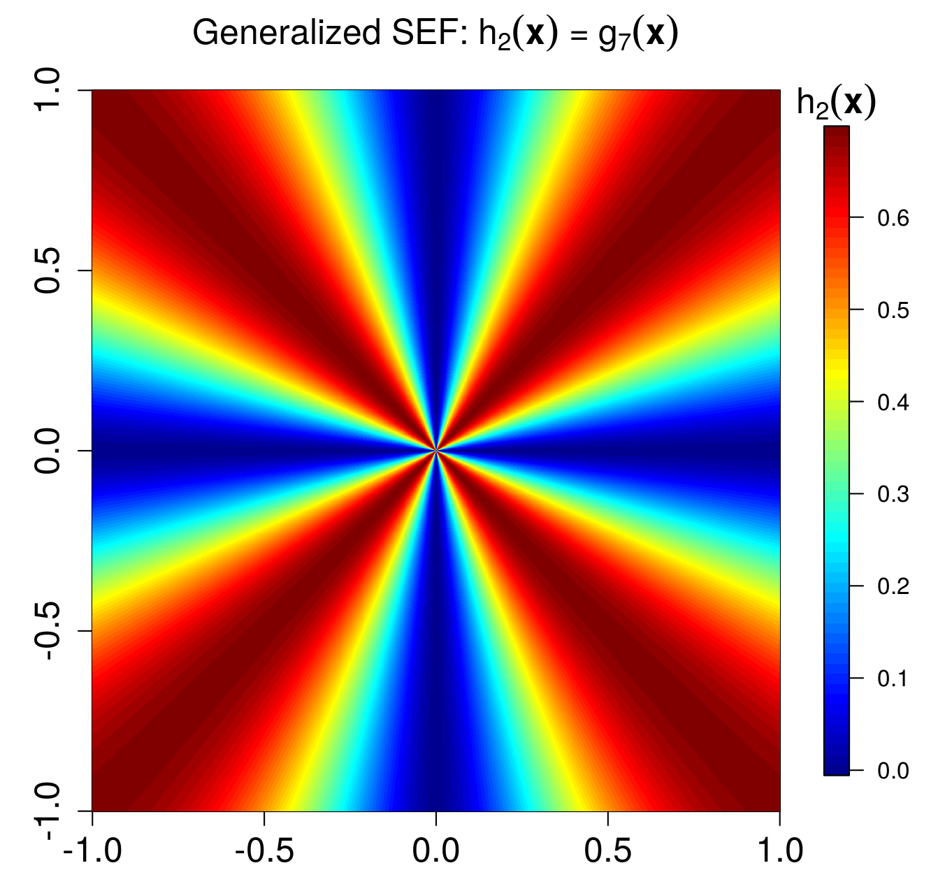
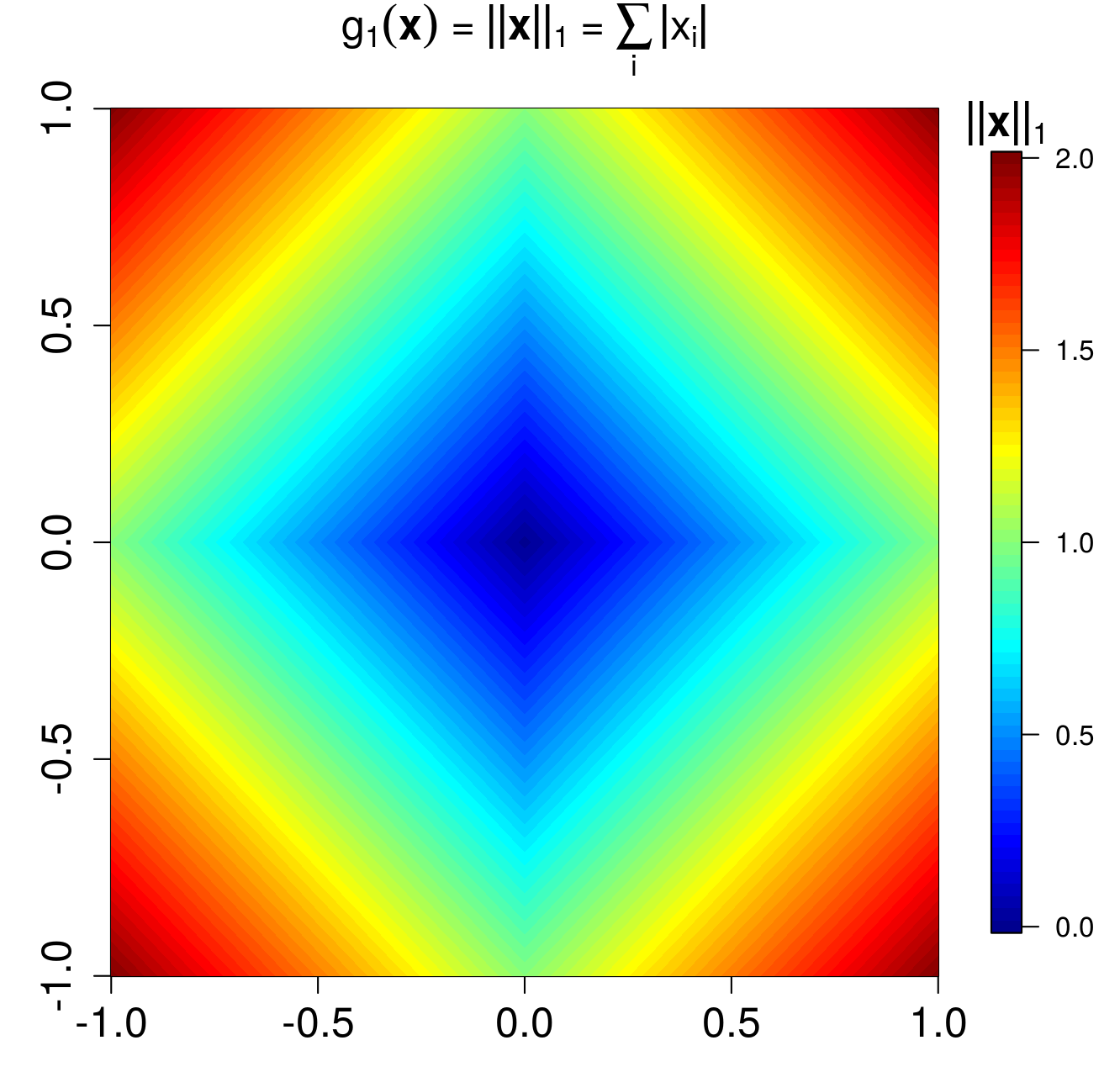
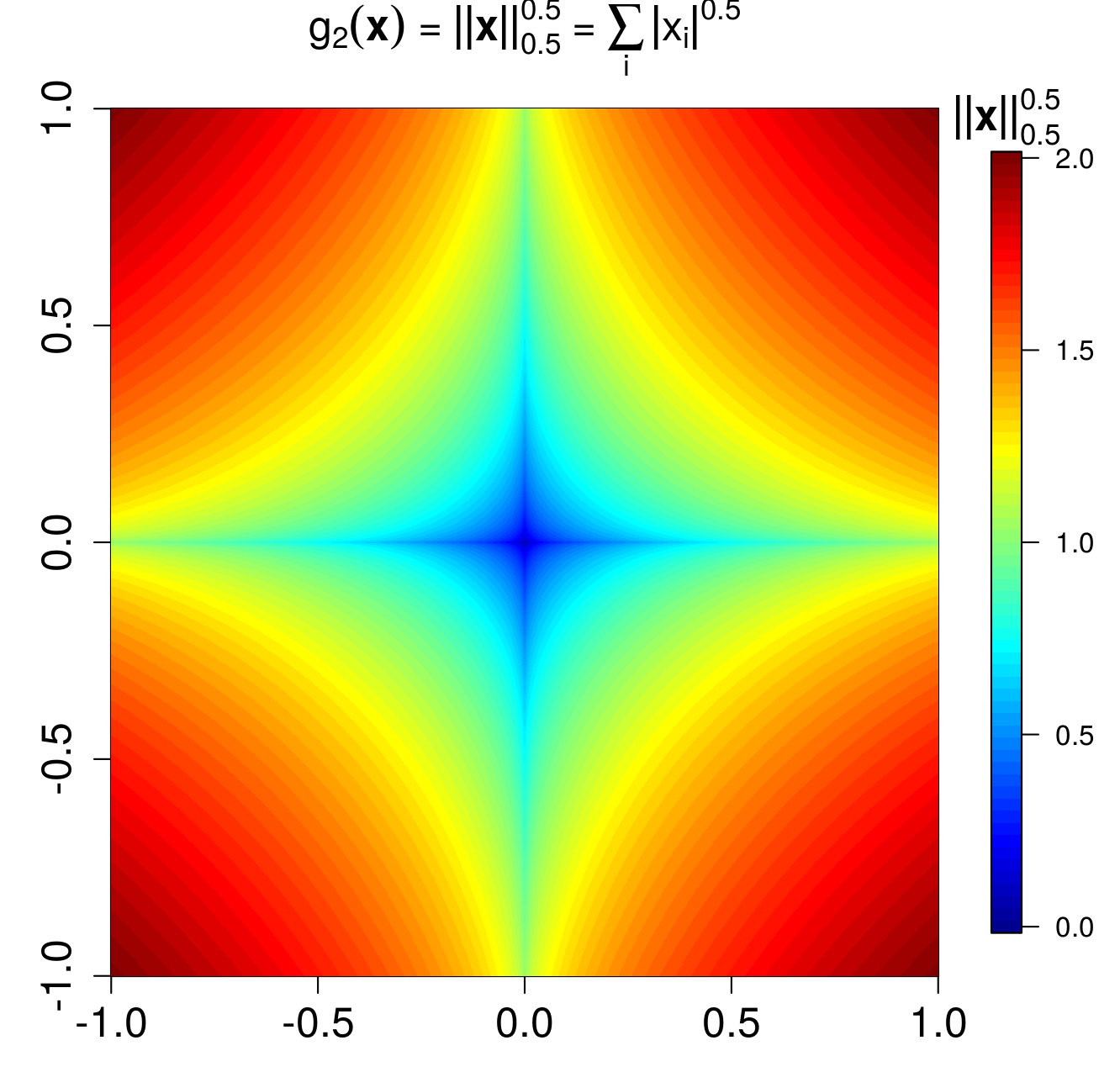
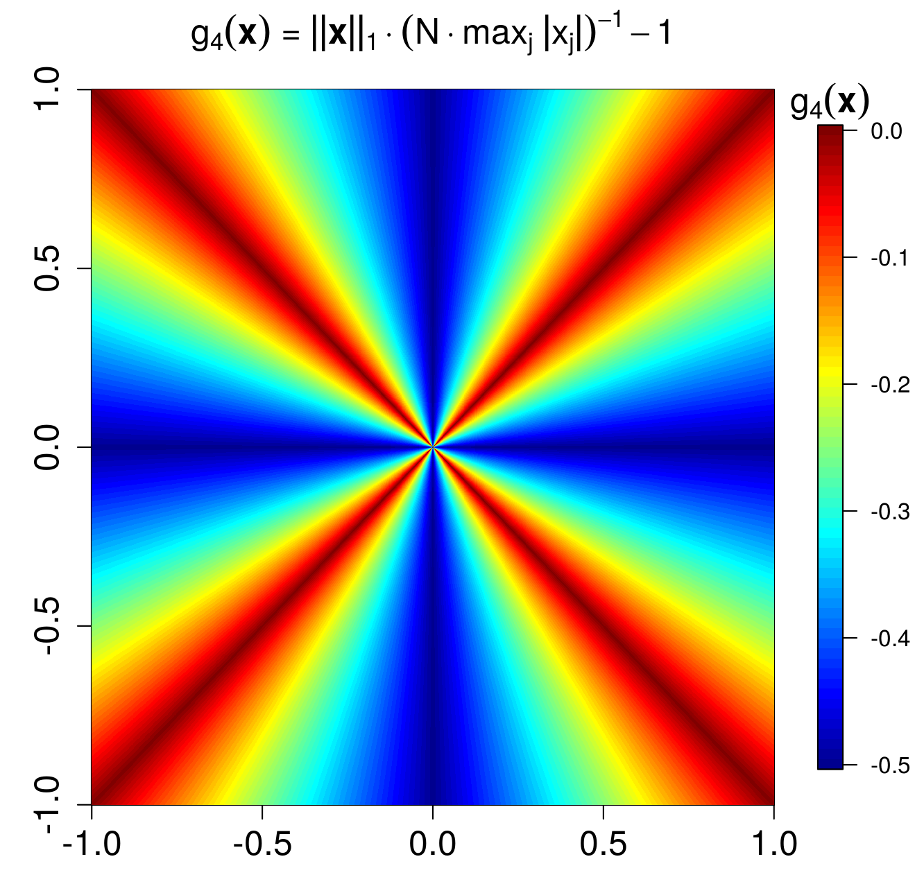
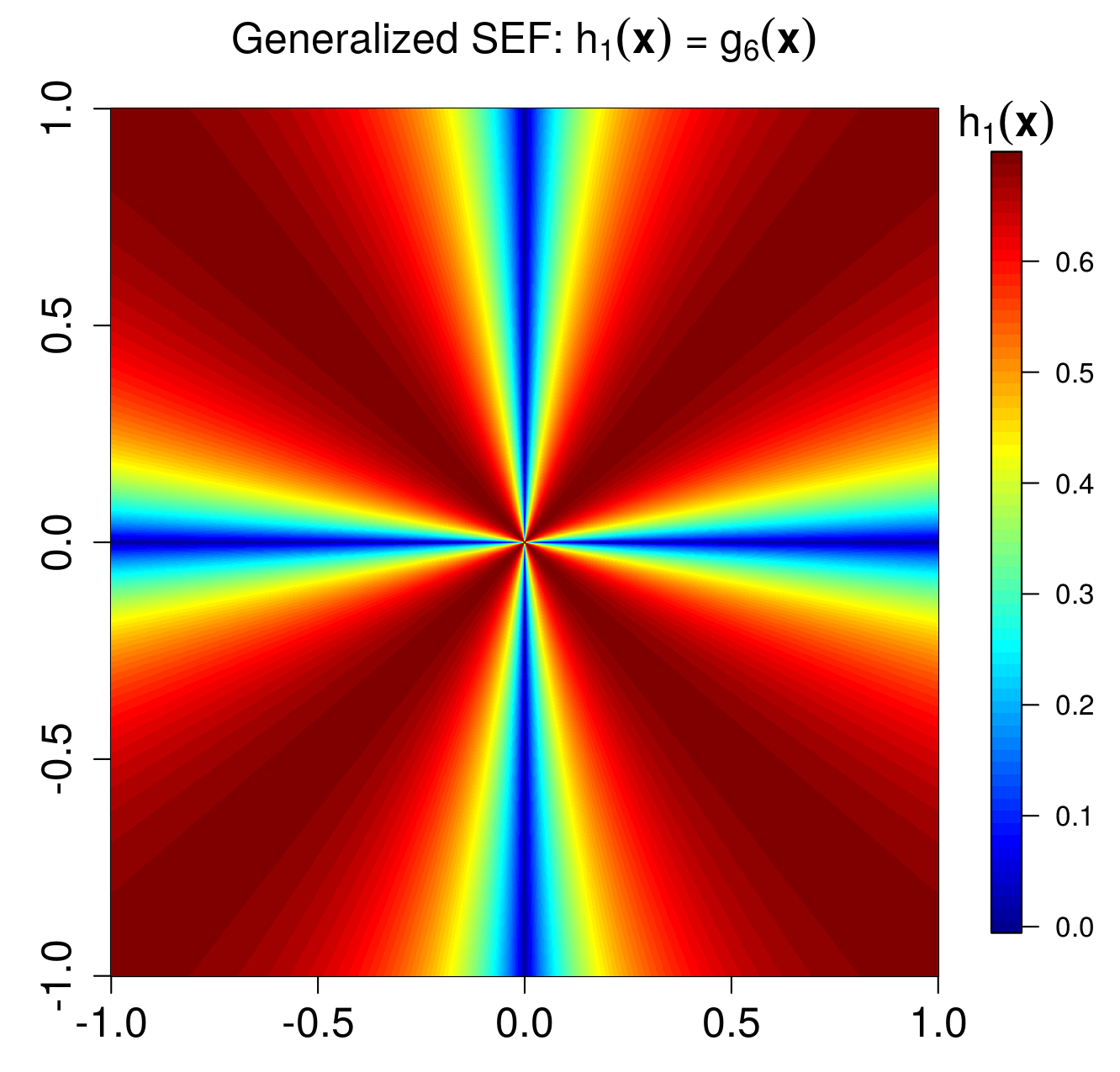
Figure 1: The proposed generalized Shannon entropy function (SEF) hp(𝒙)subscript𝑝𝒙h_{p}({\bm{x}}) compared with various sparsity-promoting regularization functions introduced in section I-A1 in 2superscript2\mathbb{R}^{2}.

Alternatively, we could impose an upper bound S+𝑆superscriptS\in\mathbb{N}^{+} on the sparsity level of 𝒙𝒙{\bm{x}}, and minimize the data fidelity term:

P0S(𝒙):min𝒙𝒚𝑨𝒙22subject to 𝒙0S.\displaystyle P_{0}^{S}({\bm{x}}):\quad\min_{{\bm{x}}}\,\|{\bm{y}}-{\bm{A}}{\bm{x}}\|_{2}^{2}\quad\textnormal{subject to }\|{\bm{x}}\|_{0}\leq S\,. (3)

Both P0ϵ(𝒙)superscriptsubscript𝑃0italic-ϵ𝒙P_{0}^{\epsilon}({\bm{x}}) and P0S(𝒙)superscriptsubscript𝑃0𝑆𝒙P_{0}^{S}({\bm{x}}) are nonconvex NP-hard problems in general [8, 9]. The l0subscript𝑙0l_{0} norm can also be used as a regularizer [10], which gives rise to the following unconstrained problem:

P0λ(𝒙):min𝒙𝒚𝑨𝒙22+λ𝒙0,\displaystyle P_{0}^{\lambda}({\bm{x}}):\quad\min_{{\bm{x}}}\,\|{\bm{y}}-{\bm{A}}{\bm{x}}\|_{2}^{2}+\lambda\|{\bm{x}}\|_{0}\,, (4)

where λ>0𝜆0\lambda>0 is the regularization parameter.

In practice, the following two approaches are usually employed to solve the sparse signal recovery problem:

  1. 1.

    Minimization of the l0subscript𝑙0l_{0} norm 𝒙0subscriptnorm𝒙0\|{\bm{x}}\|_{0}.

    • Various pursuit methods directly search for the nonzero entries of 𝒙𝒙{\bm{x}} incrementally or collectively.

      Let 𝒙~~𝒙\widetilde{{\bm{x}}} denote the nonzero entries and 𝑨~~𝑨\widetilde{{\bm{A}}} denote the corresponding support set, matching pursuit (MP) [11] greedily searches for the sparsest representation of 𝒚𝒚{\bm{y}} by adding one column of 𝑨𝑨{\bm{A}} to 𝑨~~𝑨\widetilde{{\bm{A}}} at a time until the residue is no larger than ϵitalic-ϵ\epsilon or 𝒙0subscriptnorm𝒙0\|{\bm{x}}\|_{0} reaches S𝑆S. The corresponding coefficient is also added to 𝒙~~𝒙\widetilde{{\bm{x}}} one by one during the process. Orthogonal matching pursuit [12, 13] is an extension of MP, it updates all the coefficients in 𝒙~~𝒙\widetilde{{\bm{x}}} with the orthogonal projection of 𝒚𝒚{\bm{y}} onto 𝑨~~𝑨\widetilde{{\bm{A}}} in every iteration.

      If the sparsity level S𝑆S is known, the support set 𝑨~~𝑨\widetilde{{\bm{A}}} can be further updated collectively during every iteration using CoSaMP [14] or subspace pursuit [15].

    • In an effort to solve (3) and (4), Blumensath and Davis [10, 16, 17] proposed the iterative hard thresholding (IHT) to refine the solution 𝒙(t+1)superscript𝒙𝑡1{\bm{x}}^{(t+1)} iteratively:

      𝒙(t+1)=H(𝒙(t)+𝑨T(𝒚𝑨𝒙(t))),superscript𝒙𝑡1Hsuperscript𝒙𝑡superscript𝑨T𝒚𝑨superscript𝒙𝑡\displaystyle{\bm{x}}^{(t+1)}=\textnormal{H}\left({\bm{x}}^{(t)}+{\bm{A}}^{\textnormal{T}}({\bm{y}}-{\bm{A}}{\bm{x}}^{(t)})\right)\,, (5)

      where H(𝒙)H𝒙\textnormal{H}({\bm{x}}) is a nonlinear operator defined as follows:

      1. a)

        HS(𝒙)subscriptH𝑆𝒙\textnormal{H}_{S}({\bm{x}}) preserves the largest S𝑆S entries of 𝒙𝒙{\bm{x}} in magnitude and sets the rest to 00.

      2. b)

        Hλ(𝒙)subscriptH𝜆𝒙\textnormal{H}_{\lambda}({\bm{x}}) preserves the entries whose magnitude is no less than λ𝜆\lambda and sets the rest to 00.

      The convergence of IHT is guaranteed provided that the operator norm 𝑨2subscriptnorm𝑨2\|{\bm{A}}\|_{2} is less than 111 [16]. IHT can be generalized to recover a row-sparse matrix 𝑿𝑿{\bm{X}} [18].

    The various pursuit methods and IHT can be further modified under the oblique pursuits framework [19] to work with a wider class of measurement matrices.

  2. 2.

    Relaxation of the l0subscript𝑙0l_{0} norm 𝒙0subscriptnorm𝒙0\|{\bm{x}}\|_{0}.

    The relaxed alternative objective functions should be able to quantify the sparsity level of 𝒙𝒙{\bm{x}} and easy to optimize [20]. A detailed introduction is deferred to section I-A1.

Here we focus on studying the “relaxation” approach that solves the following unconstrained recovery problem:

Pg(𝒙):min𝒙𝒚𝑨𝒙22+λg(𝒙),\displaystyle P_{g}({\bm{x}}):\quad\min_{{\bm{x}}}\,\|{\bm{y}}-{\bm{A}}{\bm{x}}\|_{2}^{2}+\lambda\,g({\bm{x}})\,, (6)

where λ>0𝜆0\lambda>0 is the parameter that balances the trade-off between the data fidelity term 𝒚𝑨𝒙22superscriptsubscriptnorm𝒚𝑨𝒙22\|{\bm{y}}-{\bm{A}}{\bm{x}}\|_{2}^{2} and the sparsity regularizer g(𝒙)𝑔𝒙g({\bm{x}}). The sparse prior is enforced via the regularizer g(𝒙)𝑔𝒙g({\bm{x}}). A proper g(𝒙)𝑔𝒙g({\bm{x}}) is crucial to the success of the sparse signal recovery task: it should favor sparse solutions, and the corresponding problem Pg(𝒙)subscript𝑃𝑔𝒙P_{g}({\bm{x}}) can be solved efficiently.

Built upon our earlier work in [21], in this paper we propose the following generalized Shannon entropy function and Rényi entropy function as new sparsity-promoting regularizers:

  1. 1.

    Shannon entropy function:

    hp(𝒙)=i=1N|xi|p𝒙pplog|xi|p𝒙pp,subscript𝑝𝒙superscriptsubscript𝑖1𝑁superscriptsubscript𝑥𝑖𝑝subscriptsuperscriptnorm𝒙𝑝𝑝superscriptsubscript𝑥𝑖𝑝subscriptsuperscriptnorm𝒙𝑝𝑝\displaystyle h_{p}({\bm{x}})=-\sum_{i=1}^{N}\frac{|x_{i}|^{p}}{\|{\bm{x}}\|^{p}_{p}}\log\frac{|x_{i}|^{p}}{\|{\bm{x}}\|^{p}_{p}}\,, (7)

    where p>0𝑝0p>0.

  2. 2.

    Rényi entropy function:

    hp,α(𝒙)=11αlog(i=1N(|xi|p𝒙pp)α),subscript𝑝𝛼𝒙11𝛼superscriptsubscript𝑖1𝑁superscriptsuperscriptsubscript𝑥𝑖𝑝superscriptsubscriptnorm𝒙𝑝𝑝𝛼\displaystyle h_{p,\alpha}({\bm{x}})=\frac{1}{1-\alpha}\log\left(\sum_{i=1}^{N}\left(\frac{|x_{i}|^{p}}{\|{\bm{x}}\|_{p}^{p}}\right)^{\alpha}\right)\,, (8)

    where p>0𝑝0p>0, α>0𝛼0\alpha>0 and α1𝛼1\alpha\neq 1.

Both hp(𝒙)subscript𝑝𝒙h_{p}({\bm{x}}) and hp,α(𝒙)subscript𝑝𝛼𝒙h_{p,\alpha}({\bm{x}}) are nonconvex functions, scale-independent, and their local minimums occur at the boundary of each orthant in the Euclidean space Nsuperscript𝑁\mathbb{R}^{N}, i.e. the axes. They share similar structures in Nsuperscript𝑁\mathbb{R}^{N}. Take the Shannon entropy function for example, the 2D level plots of hp(𝒙)subscript𝑝𝒙h_{p}({\bm{x}}) with p={1, 2}𝑝12p=\{1,\,2\} are shown in Fig. 1. In this paper we show their advantages over other popular regularizers in promoting sparse solutions with both theoretical analyses and experimental evaluations.

TABLE I: Prior entropy-based functionals.
g6(𝒙)subscript𝑔6𝒙g_{6}({\bm{x}})[22] g7(𝒙)subscript𝑔7𝒙g_{7}({\bm{x}})[23, 24, 22, 25] g8(𝒙)subscript𝑔8𝒙g_{8}({\bm{x}})[26] g9(𝒙)subscript𝑔9𝒙g_{9}({\bm{x}})[22]
i|xi|𝒙1log|xi|𝒙1subscript𝑖subscript𝑥𝑖subscriptnorm𝒙1subscript𝑥𝑖subscriptnorm𝒙1-\sum_{i}\frac{|x_{i}|}{\|{\bm{x}}\|_{1}}\log\frac{|x_{i}|}{\|{\bm{x}}\|_{1}} i|xi|2𝒙22log|xi|2𝒙22subscript𝑖superscriptsubscript𝑥𝑖2superscriptsubscriptnorm𝒙22superscriptsubscript𝑥𝑖2superscriptsubscriptnorm𝒙22-\sum_{i}\frac{|x_{i}|^{2}}{\|{\bm{x}}\|_{2}^{2}}\log\frac{|x_{i}|^{2}}{\|{\bm{x}}\|_{2}^{2}} i|xi|log|xi|subscript𝑖subscript𝑥𝑖subscript𝑥𝑖-\sum_{i}|x_{i}|\log|x_{i}| i|xi|2log|xi|2subscript𝑖superscriptsubscript𝑥𝑖2superscriptsubscript𝑥𝑖2-\sum_{i}|x_{i}|^{2}\log|x_{i}|^{2}
𝒙N𝒙superscript𝑁{\bm{x}}\in\mathbb{R}^{N}, 𝒙0𝒙0{\bm{x}}\neq 0 𝒙N𝒙superscript𝑁{\bm{x}}\in\mathbb{R}^{N}, 𝒙0𝒙0{\bm{x}}\neq 0 𝒙N𝒙superscript𝑁{\bm{x}}\in\mathbb{R}^{N}, 𝒙1subscriptnorm𝒙1\|{\bm{x}}\|_{1} is fixed. 𝒙N𝒙superscript𝑁{\bm{x}}\in\mathbb{R}^{N}, 𝒙22superscriptsubscriptnorm𝒙22\|{\bm{x}}\|_{2}^{2} is fixed.

I-A Prior Work

I-A1 Sparsity-promoting regularizers

Various regularizers have been proposed as the relaxations of the l0subscript𝑙0l_{0} norm.

  1. a)

    Most popular among them are the lpsubscript𝑙𝑝l_{p}-norm based functions, i.e. the convex l1subscript𝑙1l_{1} norm 𝒙1subscriptnorm𝒙1\|{\bm{x}}\|_{1} [24, 26, 27] and the nonconvex p𝑝p-th power of the lpsubscript𝑙𝑝l_{p} norm 𝒙ppsuperscriptsubscriptnorm𝒙𝑝𝑝\|{\bm{x}}\|_{p}^{p}, 0<p<10𝑝10<p<1 [25, 28, 29, 30]:

    • g1(𝒙)=𝒙1=i|xi|subscript𝑔1𝒙subscriptnorm𝒙1subscript𝑖subscript𝑥𝑖g_{1}({\bm{x}})=\|{\bm{x}}\|_{1}=\sum_{i}|x_{i}|, where 𝒙N𝒙superscript𝑁{\bm{x}}\in\mathbb{R}^{N}.

    • g2(𝒙)=𝒙pp=i|xi|psubscript𝑔2𝒙superscriptsubscriptnorm𝒙𝑝𝑝subscript𝑖superscriptsubscript𝑥𝑖𝑝g_{2}({\bm{x}})=\|{\bm{x}}\|_{p}^{p}=\sum_{i}|x_{i}|^{p}, where 𝒙N𝒙superscript𝑁{\bm{x}}\in\mathbb{R}^{N}, p(0,1)𝑝01p\in(0,1).

    Both 𝒙1subscriptnorm𝒙1\|{\bm{x}}\|_{1} and 𝒙ppsuperscriptsubscriptnorm𝒙𝑝𝑝\|{\bm{x}}\|_{p}^{p} are additive separable functions, and strict error bounds can be established for the recovered solutions from l1subscript𝑙1l_{1}-minimization [4, 5, 6, 7] and lppsuperscriptsubscript𝑙𝑝𝑝l_{p}^{p}-minimization problems [28, 31, 29]. Compared to l1subscript𝑙1l_{1}-minimization, lppsuperscriptsubscript𝑙𝑝𝑝l_{p}^{p}-minimization has a tighter error bound and better sparse recovery performances.

  2. b)

    When 𝒙𝒙{\bm{x}} lies in the probability simplex, i.e. 𝒙1=1subscriptnorm𝒙11\|{\bm{x}}\|_{1}=1 and xi0,isubscript𝑥𝑖0for-all𝑖x_{i}\geq 0,\forall i, minimizing 𝒙1subscriptnorm𝒙1\|{\bm{x}}\|_{1} would not work in this case. [32] proposed a lower bound g3(𝒙)subscript𝑔3𝒙g_{3}({\bm{x}}) on 𝒙0subscriptnorm𝒙0\|{\bm{x}}\|_{0}, and showed that the optimization problem can be efficiently solved using convex programming:

    • g3(𝒙)=1𝒙=1maxjxj𝒙0subscript𝑔3𝒙1subscriptnorm𝒙1subscript𝑗subscript𝑥𝑗subscriptnorm𝒙0g_{3}({\bm{x}})=\frac{1}{\|{\bm{x}}\|_{\infty}}=\frac{1}{\max_{j}x_{j}}\leq\|{\bm{x}}\|_{0},

      where 𝒙>𝟎𝒙0{\bm{x}}>\bm{0}, 𝒙1=1subscriptnorm𝒙11\|{\bm{x}}\|_{1}=1.

    [33] later proposed the following sparsity regularizer111The sparsity measure proposed in [33] is actually g4(𝒙)subscript𝑔4𝒙-g_{4}({\bm{x}}). The sign is flipped because we are minimizing the regularizer here.:

    • g4(𝒙)=𝒙1N𝒙1=𝒙1Nmaxj|xj|1subscript𝑔4𝒙subscriptnorm𝒙1𝑁subscriptnorm𝒙1subscriptnorm𝒙1𝑁subscript𝑗subscript𝑥𝑗1g_{4}({\bm{x}})=\frac{\|{\bm{x}}\|_{1}}{N\cdot\|{\bm{x}}\|_{\infty}}-1=\frac{\|{\bm{x}}\|_{1}}{N\cdot\max_{j}|x_{j}|}-1,

      where 𝒙N𝒙superscript𝑁{\bm{x}}\in\mathbb{R}^{N}, 𝒙𝟎𝒙0{\bm{x}}\neq\bm{0}.

    When 𝒙1=1subscriptnorm𝒙11\|{\bm{x}}\|_{1}=1 and 𝒙>0𝒙0{\bm{x}}>0, minimizing g4(𝒙)subscript𝑔4𝒙g_{4}({\bm{x}}) is equivalent to minimizing g3(𝒙)subscript𝑔3𝒙g_{3}({\bm{x}}). The function g3(𝒙)subscript𝑔3𝒙g_{3}({\bm{x}}) could be considered to be a modified special case of g4(𝒙)subscript𝑔4𝒙g_{4}({\bm{x}}). For readability purposes, we shall refer to g4(𝒙)subscript𝑔4𝒙g_{4}({\bm{x}}) as the “L1/LsubscriptL1subscriptL\textnormal{L}_{1}/\textnormal{L}_{\infty}” function in this paper.

    Although the L1/LsubscriptL1subscriptL\textnormal{L}_{1}/\textnormal{L}_{\infty} function and the proposed hp(𝒙)subscript𝑝𝒙h_{p}({\bm{x}}), hp,α(𝒙)subscript𝑝𝛼𝒙h_{p,\alpha}({\bm{x}}) are all scale-independent (see Fig. 1 for a 2D example), they differ in the following aspects:

    • The proposed entropy functions are continuously differentiable w.r.t. the modulus |𝒙|𝒙|{\bm{x}}|, while the L1/LsubscriptL1subscriptL\textnormal{L}_{1}/\textnormal{L}_{\infty} function is not.

    • The proposed entropy functions have adaptive energy-promoting behaviors, while the L1/LsubscriptL1subscriptL\textnormal{L}_{1}/\textnormal{L}_{\infty} function has a rigid energy-promoting behavior. The detailed analysis is presented in section II-D and Appendix B.

  3. c)

    Another popular class of regularizers is constructed from the logarithm function log()\log(\cdot) [24, 34, 35, 25]. The following “logarithm of energy” function was proposed in [24] as a measure of sparsity:

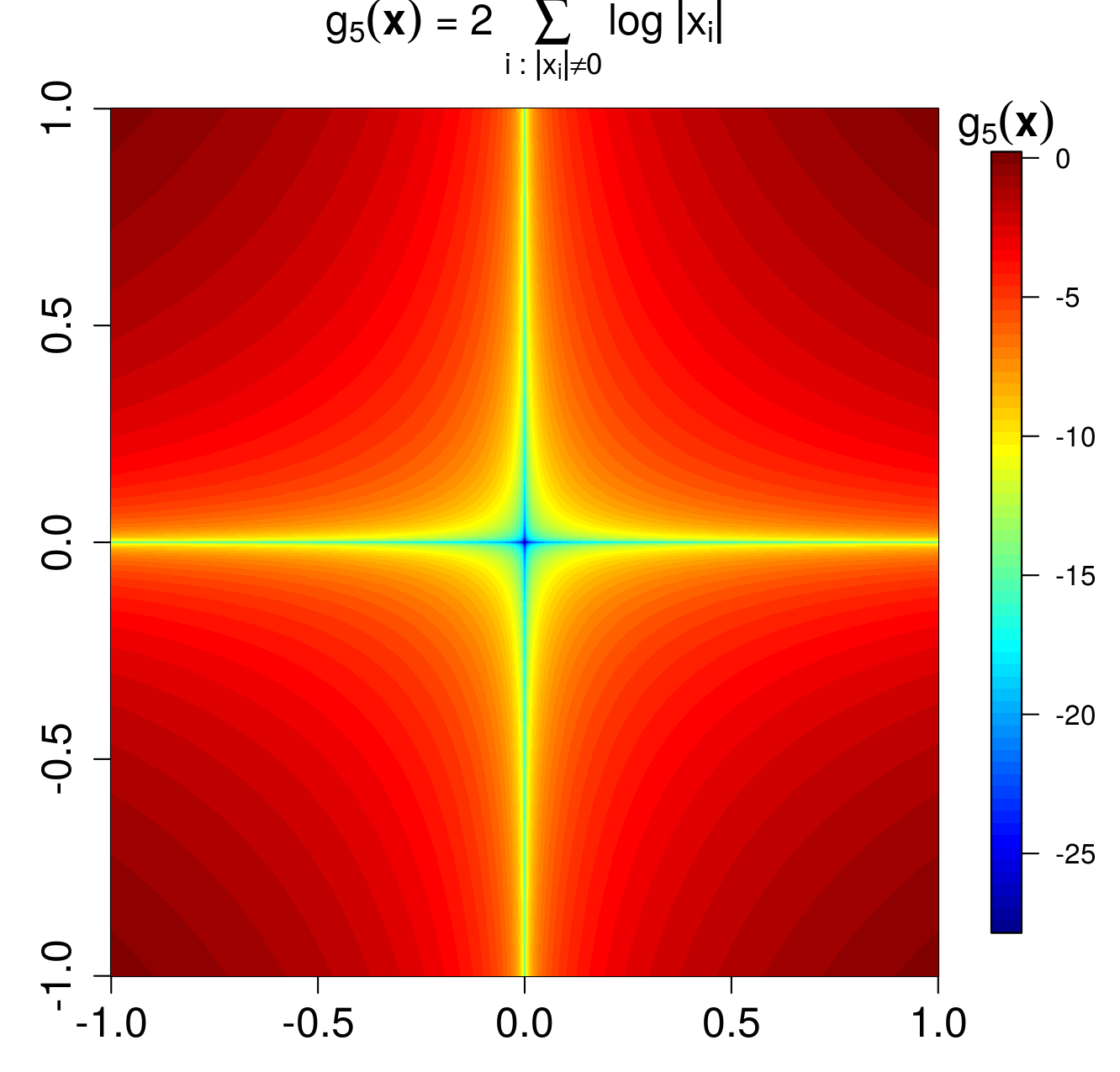
    • g5(𝒙)=i:|xi|0log|xi|2=2i:|xi|0log|xi|subscript𝑔5𝒙subscript:𝑖subscript𝑥𝑖0superscriptsubscript𝑥𝑖22subscript:𝑖subscript𝑥𝑖0subscript𝑥𝑖g_{5}({\bm{x}})=\sum_{i:|x_{i}|\neq 0}\log|x_{i}|^{2}=2\sum_{i:|x_{i}|\neq 0}\log|x_{i}|, where 𝒙N𝒙superscript𝑁{\bm{x}}\in\mathbb{R}^{N}, 𝒙𝟎𝒙0{\bm{x}}\neq\bm{0}.

    Candès et al. [36] later proposed the reweighted l1subscript𝑙1l_{1}-minimization algorithm as a way to enhance the sparsity, which is essentially the iterative minimization of the first-order approximation of g5(𝒙)subscript𝑔5𝒙g_{5}({\bm{x}}): ilog(|xi|+ϵ)subscript𝑖subscript𝑥𝑖italic-ϵ\sum_{i}\log(|x_{i}|+\epsilon), where ϵ>0italic-ϵ0\epsilon>0 is some small positive constant.

  4. d)

    As listed in Table I, entropy-based functionals have also been widely used to promote sparsity in 𝒙𝒙{\bm{x}}. Specifically, g6(𝒙)subscript𝑔6𝒙g_{6}({\bm{x}}) and g7(𝒙)subscript𝑔7𝒙g_{7}({\bm{x}}) are special cases of the proposed generalized Shannon entropy function hp(𝒙)subscript𝑝𝒙h_{p}({\bm{x}}) in (7) when p=1𝑝1p=1 and 222. There is some imprecision in [22]’s analysis on the local minimums of g7(𝒙)subscript𝑔7𝒙g_{7}({\bm{x}}), which were believed to “occur just shy of the boundaries defined by the coordinate axes”. In section II-C, we can prove that the local minimums actually occur exactly on the coordinate axes. g8(𝒙)subscript𝑔8𝒙g_{8}({\bm{x}}) only promotes sparsity if the signal 𝒙𝒙{\bm{x}} has fixed l1subscript𝑙1l_{1} norm, while g9(𝒙)subscript𝑔9𝒙g_{9}({\bm{x}}) works for signals with fixed l2subscript𝑙2l_{2} norm.

  5. e)

    The functions g6(𝒙)subscript𝑔6𝒙g_{6}({\bm{x}}), \cdots, g9(𝒙)subscript𝑔9𝒙g_{9}({\bm{x}}) are all nonconvex. [37] later proposed the following convex entropy function as an approximation to the l1subscript𝑙1l_{1}-norm 𝒙1subscriptnorm𝒙1\|{\bm{x}}\|_{1}:

    • g10(𝒙)=i[(|xi|+e1)log(|xi|+e1)+e1]subscript𝑔10𝒙subscript𝑖delimited-[]subscript𝑥𝑖superscript𝑒1subscript𝑥𝑖superscript𝑒1superscript𝑒1g_{10}({\bm{x}})=\sum_{i}\left[(|x_{i}|+e^{-1})\log(|x_{i}|+e^{-1})\,+\,e^{-1}\right],
      where 𝒙N𝒙superscript𝑁{\bm{x}}\in\mathbb{R}^{N}.

    This way g10(𝒙)subscript𝑔10𝒙g_{10}({\bm{x}}) maintains the strictly convex property of 𝒙1subscriptnorm𝒙1\|{\bm{x}}\|_{1} and is continuously differentiable in Nsuperscript𝑁\mathbb{R}^{N}. However, we should note that g10(𝒙)subscript𝑔10𝒙g_{10}({\bm{x}}) only produces concentrated but not truly sparse solutions.

I-A2 l1subscript𝑙1l_{1}-norm minimization algorithms

When g(𝒙)=𝒙1𝑔𝒙subscriptnorm𝒙1g({\bm{x}})=\|{\bm{x}}\|_{1}, the convex l1subscript𝑙1l_{1}-norm minimization problem can be efficiently solved using various readily available algorithms such as GPSR [38], ISTA [39, 40, 41], TwIST[42], FISTA [43, 44], NESTA [45, 46], ADM[47], etc. Detailed reviews of popular l1subscript𝑙1l_{1}-norm minimization algorithms can be found in [48, 49].

In this paper the optimization problem (6) is recasted into a series of reweighted l1subscript𝑙1l_{1} problems [36, 30]. We choose to adapt the FISTA to solve (6) for its easy implementation and fast convergence.

I-A3 Uniqueness of the solution

The restricted isometry property (RIP) of the M×N𝑀𝑁M\times N sensing matrix 𝑨𝑨{\bm{A}} was introduced in [4] to provide guarantees for exact recovery. Let δSsubscript𝛿𝑆\delta_{S} be the smallest number such that:

(1δS)𝒙22𝑨𝒙22(1+δS)𝒙22.1subscript𝛿𝑆superscriptsubscriptnorm𝒙22superscriptsubscriptnorm𝑨𝒙221subscript𝛿𝑆superscriptsubscriptnorm𝒙22\displaystyle(1-\delta_{S})\|{\bm{x}}\|_{2}^{2}\leq\|{\bm{A}}{\bm{x}}\|_{2}^{2}\leq(1+\delta_{S})\|{\bm{x}}\|_{2}^{2}\,. (9)

holds for all vectors 𝒙𝒙{\bm{x}} with 𝒙0Ssubscriptnorm𝒙0𝑆\|{\bm{x}}\|_{0}\leq S, then the matrix 𝑨𝑨{\bm{A}} is said to satisfy RIP with S𝑆S-restricted constant δSsubscript𝛿𝑆\delta_{S}. In the noiseless case [7], when δ2S<21subscript𝛿2𝑆21\delta_{2S}<\sqrt{2}-1, minimizing the convex relaxation 𝒙1subscriptnorm𝒙1\|{\bm{x}}\|_{1} is equivalent to minimizing the nonconvex 𝒙0subscriptnorm𝒙0\|{\bm{x}}\|_{0}, and has a unique S𝑆S-sparse solution. In the noisy case [7], a strict upper bound on the l2subscript𝑙2l_{2} error 𝒙^𝒙norm^𝒙𝒙\|\hat{{\bm{x}}}-{\bm{x}}\| of the recovered 𝒙1subscriptnorm𝒙1\|{\bm{x}}\|_{1}-minimization solution 𝒙^^𝒙\hat{{\bm{x}}} can be established.

It was shown in [7] that the RIP can be met with high probability for Gaussian random matrix with i.i.d entries and M>CSlog(N/S)𝑀𝐶𝑆𝑁𝑆M>CS\log(N/S) for some constant C𝐶C. Chartrand et al. [28, 31] later gave the uniqueness conditions for 𝒙ppsuperscriptsubscriptnorm𝒙𝑝𝑝\|{\bm{x}}\|_{p}^{p}-minimization in terms of the RIP of 𝑨𝑨{\bm{A}}. Both 𝒙1subscriptnorm𝒙1\|{\bm{x}}\|_{1} and 𝒙ppsuperscriptsubscriptnorm𝒙𝑝𝑝\|{\bm{x}}\|_{p}^{p} are additive separable functions in that they can be written as a sum of identical functions involving individual entries of 𝒙𝒙{\bm{x}}. However, the proposed entropy functions are non-separable, and different approaches are needed to find the properties of 𝑨𝑨{\bm{A}} that could guarantee the uniqueness of the solution.

I-B Main Contributions

Compared to previously adapted entropy functions [23, 24, 22, 25] where only l1subscript𝑙1l_{1} and l22superscriptsubscript𝑙22l_{2}^{2} normalized 𝒙𝒙{\bm{x}} were studied, the proposed Shannon entropy function hp(𝒙)subscript𝑝𝒙h_{p}({\bm{x}}) and Rényi entropy function hp,α(𝒙)subscript𝑝𝛼𝒙h_{p,\alpha}({\bm{x}}) in (7, 8) are more general. They are defined with respect to the probability distribution in (12) where p>0𝑝0p>0 can be any positive number. This gives us more freedom in constructing the proper entropy functions for the sparse signal recovery task. As evident from the experiments on both simulated and real data, the ability to choose suitable p𝑝p values enables us to fully exploit the sparsity-promoting power of the generalized entropy functions and to achieve better performances over other state-of-the-art regularized approaches.

Previous works [22, 25] focused on the study of the Schur concavity of the generalized entropy functions with respect to 𝒙𝒙{\bm{x}} where p=1, 2𝑝12p=1,\,2. They believed that the Shannon entropy function produced truly sparse solutions only when p=1𝑝1p=1. Here we show that it’s actually the (Schur) concavity with respect to the distribution 𝒫()𝒫\mathscr{P}(\cdot) that really matters. The Shannon entropy function with p=1𝑝1p=1 is not the only case where truly sparse solutions can be obtained. In fact, p>0for-all𝑝0\forall\,p>0 and 0<α10𝛼10<\alpha\neq 1, we can prove in section II-C that the local minimums of the generalized entropy functions only occur at the boundaries of the orthants in Nsuperscript𝑁\mathbb{R}^{N}. Hence minimizing hp(𝒙)subscript𝑝𝒙h_{p}({\bm{x}}) or hp,α(𝒙)subscript𝑝𝛼𝒙h_{p,\alpha}({\bm{x}}) in said orthant 𝕆𝕆\mathbb{O} will lead us to the solutions on its boundary, i.e. sparser solutions.

Additionally, minimizing the generalized entropy functions adaptively promotes multiple high-energy coefficients while suppressing the rest low-energy coefficients. Combining the proximal approximation [50, 51] of the data fidelity term and the first order approximations of the generalized entropy functions, we can recast the nonconvex entropy functions minimization problems into a series of simple reweighted l1subscript𝑙1l_{1} problems, and solve them efficiently via the accelerated inexact proximal gradient method [43, 44, 52].

II Sparsity-Regularization Entropy Functions

II-A Entropy in Information Theory

Here we first introduce the entropy concepts in information theory [53, 54]. Both the Shannon entropy and Rényi entropy are defined with respect to the probability distribution 𝓟(𝒱)𝓟𝒱\bm{\mathscr{P}}(\mathcal{V}) of some random variable 𝒱𝒱\mathcal{V}. We give the definitions in terms of discrete probability distribution222For continuous distributions, the sum \sum in (10,11) should be replaced with integration \int. as follows:

  • Shannon entropy333The “log\log” in this paper is by default natural logarithm, i.e. base e𝑒e:

    (𝒱)=i=1|𝒱|𝒫(vi)log𝒫(vi).𝒱superscriptsubscript𝑖1𝒱𝒫subscript𝑣𝑖𝒫subscript𝑣𝑖\displaystyle\mathcal{H}(\mathcal{V})=-\textstyle\sum_{i=1}^{|\mathcal{V}|}\mathscr{P}(v_{i})\log\mathscr{P}(v_{i})\,. (10)

    (𝒱)𝒱\mathcal{H}(\mathcal{V}) is strictly concave with respect to the probability distribution 𝓟(𝒱)={𝒫(v1),,𝒫(v|𝒱|)}𝓟𝒱𝒫subscript𝑣1𝒫subscript𝑣𝒱\bm{\mathscr{P}}(\mathcal{V})=\{\mathscr{P}(v_{1}),\cdots,\mathscr{P}(v_{|\mathcal{V}|})\}.

  • Rényi entropy:

    α(𝒱)=11αlog(i=1|𝒱|𝒫(vi)α),subscript𝛼𝒱11𝛼superscriptsubscript𝑖1𝒱𝒫superscriptsubscript𝑣𝑖𝛼\displaystyle\mathcal{H}_{\alpha}(\mathcal{V})=\frac{1}{1-\alpha}\log\left(\textstyle\sum_{i=1}^{|\mathcal{V}|}\mathscr{P}(v_{i})^{\alpha}\right)\,, (11)

    where α0𝛼0\alpha\geq 0 and α1𝛼1\alpha\neq 1. When α(0,1)𝛼01\alpha\in(0,1), α(𝒱)subscript𝛼𝒱\mathcal{H}_{\alpha}(\mathcal{V}) is strictly concave with respect to 𝓟(𝒱)𝓟𝒱\bm{\mathscr{P}}(\mathcal{V}) [55]; when α(1,)𝛼1\alpha\in(1,\infty), α(𝒱)subscript𝛼𝒱\mathcal{H}_{\alpha}(\mathcal{V}) is strictly Schur concave with respect to 𝓟(𝒱)𝓟𝒱\bm{\mathscr{P}}(\mathcal{V}) [56].

We should make it clear that Shannon entropy (𝒱)𝒱\mathcal{H}(\mathcal{V}) is not a special case of the Rényi entropy, but the limiting value of the Rényi entropy α(𝒱)subscript𝛼𝒱\mathcal{H}_{\alpha}(\mathcal{V}) as α1𝛼1\alpha\rightarrow 1 [57]. Hence we will discuss them separately in this paper.

II-B Generalized Entropy Functions of the Sparse Signal

Entropy measures the uncertainty about the random variable 𝒱𝒱\mathcal{V} with cardinality |𝒱|=N𝒱𝑁|\mathcal{V}|=N. The lower the entropy is, the more predictable the variable 𝒱𝒱\mathcal{V} will be. This corresponds to a skewed distribution 𝓟(𝒱)𝓟𝒱\bm{\mathscr{P}}(\mathcal{V}). The idea of a skewed distribution could translate naturally to a sparse probability vector 𝓟𝒱=[𝒫(v1),,𝒫(vN)]Tsubscript𝓟𝒱superscript𝒫subscript𝑣1𝒫subscript𝑣𝑁T\bm{\mathscr{P}}_{\mathcal{V}}=\left[\mathscr{P}(v_{1}),\cdots,\mathscr{P}(v_{N})\right]^{\textnormal{T}} in the sense that only a few probability entries of 𝓟𝒱Nsubscript𝓟𝒱superscript𝑁\bm{\mathscr{P}}_{\mathcal{V}}\in\mathbb{R}^{N} are significant. In other words, the entropy can be used as a measure of how sparse the probability vector 𝓟𝒱subscript𝓟𝒱\bm{\mathscr{P}}_{\mathcal{V}} is. This observation motivates us to adapt the concept of entropy as a sparsity-measure for the general signal 𝒙𝒙{\bm{x}}, and use it as a regularizer in the sparse signal recovery task.

As mentioned before, the entropy is defined with respect to some probability distribution 𝓟()𝓟\bm{\mathscr{P}}(\cdot). Here we can construct the following discrete probability distribution out of the signal of interest 𝒙N𝒙superscript𝑁{\bm{x}}\in\mathbb{R}^{N}:

𝒙[|x1|p𝒙pp,|x2|p𝒙pp,,|xN|p𝒙pp],𝒙superscriptsubscript𝑥1𝑝superscriptsubscriptnorm𝒙𝑝𝑝superscriptsubscript𝑥2𝑝superscriptsubscriptnorm𝒙𝑝𝑝superscriptsubscript𝑥𝑁𝑝superscriptsubscriptnorm𝒙𝑝𝑝\displaystyle{\bm{x}}\rightarrow\left[\frac{|x_{1}|^{p}}{\|{\bm{x}}\|_{p}^{p}},\frac{|x_{2}|^{p}}{\|{\bm{x}}\|_{p}^{p}},\cdots,\frac{|x_{N}|^{p}}{\|{\bm{x}}\|_{p}^{p}}\right]\,, (12)

where p>0𝑝0p>0. The adaptation from the classical entropy to the generalized entropy function is then pretty straightforward: we simply plug (12) into (10) and (11) to obtain the generalized Shannon entropy function (7) and the generalized Rényi entropy function (8).

Here we should not confuse the “entropy function” of 𝒙𝒙{\bm{x}} with the “entropy” of 𝒙𝒙{\bm{x}}. Take the Shannon entropy of 𝒙𝒙{\bm{x}} for example: (𝒙)=𝒙𝒫(𝒙)log𝒫(𝒙)𝑑𝒙𝒙subscript𝒙𝒫𝒙𝒫𝒙differential-d𝒙\mathcal{H}({\bm{x}})=-\int_{{\bm{x}}}\mathscr{P}({\bm{x}})\log\mathscr{P}({\bm{x}})\,d{\bm{x}}. (𝒙)𝒙\mathcal{H}({\bm{x}}) measures the uncertainty of the random variable 𝒙𝒙{\bm{x}}, it is different from hp(𝒙)subscript𝑝𝒙h_{p}({\bm{x}}) in (7) that measures the sparsity of 𝒙𝒙{\bm{x}}.

In order to promote sparsity in the recovered solutions, we are going to minimize the generalized entropy functions. The sparse signal recovery problems in the form of (6) using the Shannon entropy function (SEF) hp(𝒙)subscript𝑝𝒙h_{p}({\bm{x}}) and the Rényi entropy function (REF) hp,α(𝒙)subscript𝑝𝛼𝒙h_{p,\alpha}({\bm{x}}) as regularizers then become:

Php(𝒙)::subscript𝑃subscript𝑝𝒙absent\displaystyle P_{h_{p}}({\bm{x}}): min𝒙𝒚𝑨𝒙22+λhp(𝒙)subscript𝒙superscriptsubscriptnorm𝒚𝑨𝒙22𝜆subscript𝑝𝒙\displaystyle\quad\min_{{\bm{x}}}\,\|{\bm{y}}-{\bm{A}}{\bm{x}}\|_{2}^{2}+\lambda\,\,h_{p}({\bm{x}}) (13)
Php,α(𝒙)::subscript𝑃subscript𝑝𝛼𝒙absent\displaystyle P_{h_{p,\alpha}}({\bm{x}}): min𝒙𝒚𝑨𝒙22+λhp,α(𝒙).subscript𝒙superscriptsubscriptnorm𝒚𝑨𝒙22𝜆subscript𝑝𝛼𝒙\displaystyle\quad\min_{{\bm{x}}}\,\|{\bm{y}}-{\bm{A}}{\bm{x}}\|_{2}^{2}+\lambda\,\,h_{p,\alpha}({\bm{x}})\,. (14)

II-C Sparsity-promoting Analysis

We next show that hp(𝒙)subscript𝑝𝒙h_{p}({\bm{x}}) and hp,α(𝒙)subscript𝑝𝛼𝒙h_{p,\alpha}({\bm{x}}) can be used as sparsity regularizers in the following sense: minimizing them in an orthant 𝕆𝕆\mathbb{O} of the Euclidean space Nsuperscript𝑁\mathbb{R}^{N} leads to solutions on the boundary of said orthant, i.e. sparser solutions.

  • ❑ Noiseless recovery:

    In this case we are minimizing hp(𝒙)subscript𝑝𝒙h_{p}({\bm{x}}) or hp,α(𝒙)subscript𝑝𝛼𝒙h_{p,\alpha}({\bm{x}}) subject to the constraint 𝒚=𝑨𝒙𝒚𝑨𝒙{\bm{y}}={\bm{A}}{\bm{x}}, 𝒚0𝒚0{\bm{y}}\neq 0. We first show that there is a one to one mapping in each orthant between 𝒙=[x1,,xN]T𝒙superscriptsubscript𝑥1subscript𝑥𝑁T{\bm{x}}=\left[x_{1},\cdots,x_{N}\right]^{\textrm{T}} and 𝒙¨=[x¨1,,x¨N]T¨𝒙superscriptsubscript¨𝑥1subscript¨𝑥𝑁T\ddot{{\bm{x}}}=\left[\ddot{x}_{1},\cdots,\ddot{x}_{N}\right]^{\textrm{T}}, where x¨i=sign(xi)|xi|p𝒙ppsubscript¨𝑥𝑖signsubscript𝑥𝑖superscriptsubscript𝑥𝑖𝑝subscriptsuperscriptnorm𝒙𝑝𝑝\ddot{x}_{i}=\textrm{sign}(x_{i})\cdot\frac{|x_{i}|^{p}}{\|{\bm{x}}\|^{p}_{p}}. This will be done in two steps: Proposition 1 and Proposition 2.

    Proposition 1.

    If 𝐱𝐱{\bm{x}} is the solution to 𝐲=𝐀𝐱𝐲𝐀𝐱{\bm{y}}={\bm{A}}{\bm{x}}, 𝐲0𝐲0{\bm{y}}\neq 0, then there is a one to one mapping in each orthant between 𝐱𝐱{\bm{x}} and 𝐱~=𝐱𝐱p~𝐱𝐱subscriptnorm𝐱𝑝\tilde{{\bm{x}}}=\frac{{\bm{x}}}{\|{\bm{x}}\|_{p}}.

    Proof.

    We need to prove 𝒙𝒙~𝒙~𝒙{\bm{x}}\longleftrightarrow\tilde{{\bm{x}}}:

    • It is easy to verify that 𝒙𝒙~𝒙~𝒙{\bm{x}}\rightarrow\tilde{{\bm{x}}}.

    • Suppose that 𝒙~~𝒙\tilde{{\bm{x}}} can be mapped to two solutions of 𝒚=𝑨𝒙𝒚𝑨𝒙{\bm{y}}={\bm{A}}{\bm{x}}: 𝒙(1),𝒙(2)subscript𝒙1subscript𝒙2{\bm{x}}_{(1)},{\bm{x}}_{(2)} in the same orthant. We then have:

      𝒙(1)𝒙(1)psubscript𝒙1subscriptnormsubscript𝒙1𝑝\displaystyle\frac{{\bm{x}}_{(1)}}{\|{\bm{x}}_{(1)}\|_{p}} =𝒙~=𝒙(2)𝒙(2)pabsent~𝒙subscript𝒙2subscriptnormsubscript𝒙2𝑝\displaystyle=\tilde{{\bm{x}}}=\frac{{\bm{x}}_{(2)}}{\|{\bm{x}}_{(2)}\|_{p}} (15)
      𝒚𝒙(1)p=𝑨𝒙(1)𝒙(1)p𝒚subscriptnormsubscript𝒙1𝑝𝑨subscript𝒙1subscriptnormsubscript𝒙1𝑝\displaystyle\frac{{\bm{y}}}{\|{\bm{x}}_{(1)}\|_{p}}=\frac{{\bm{A}}{\bm{x}}_{(1)}}{\|{\bm{x}}_{(1)}\|_{p}} =𝑨𝒙~=𝑨𝒙(2)𝒙(2)p=𝒚𝒙(2)p,absent𝑨~𝒙𝑨subscript𝒙2subscriptnormsubscript𝒙2𝑝𝒚subscriptnormsubscript𝒙2𝑝\displaystyle={\bm{A}}\tilde{{\bm{x}}}=\frac{{\bm{A}}{\bm{x}}_{(2)}}{\|{\bm{x}}_{(2)}\|_{p}}=\frac{{\bm{y}}}{\|{\bm{x}}_{(2)}\|_{p}}\,, (16)

      which tells us 𝒚𝒙(1)p=𝒚𝒙(2)p𝒚subscriptnormsubscript𝒙1𝑝𝒚subscriptnormsubscript𝒙2𝑝\frac{{\bm{y}}}{\|{\bm{x}}_{(1)}\|_{p}}=\frac{{\bm{y}}}{\|{\bm{x}}_{(2)}\|_{p}}. Since 𝒚0𝒚0{\bm{y}}\neq 0, we have 𝒙(1)p=𝒙(2)psubscriptnormsubscript𝒙1𝑝subscriptnormsubscript𝒙2𝑝\|{\bm{x}}_{(1)}\|_{p}=\|{\bm{x}}_{(2)}\|_{p}. Using (15), we get 𝒙(1)=𝒙(2)subscript𝒙1subscript𝒙2{\bm{x}}_{(1)}={\bm{x}}_{(2)}. Hence 𝒙𝒙~𝒙~𝒙{\bm{x}}\leftarrow\tilde{{\bm{x}}}.

Refer to caption
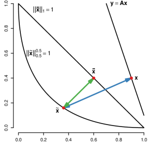
Figure 2: The one-to-one mapping in the noiseless case: 𝒙𝒙~𝒙¨𝒙~𝒙¨𝒙{\bm{x}}\longleftrightarrow\tilde{{\bm{x}}}\longleftrightarrow\ddot{{\bm{x}}} when p=0.5𝑝0.5p=0.5.
Proposition 2.

There is a one to one mapping in each orthant between 𝐱~~𝐱\tilde{{\bm{x}}} and 𝐱¨¨𝐱\ddot{{\bm{x}}}.

Proof.

We need to prove 𝒙~𝒙¨~𝒙¨𝒙\tilde{{\bm{x}}}\longleftrightarrow\ddot{{\bm{x}}}:

  • We can rewrite 𝒙¨¨𝒙\ddot{{\bm{x}}} in terms of 𝒙~~𝒙\tilde{{\bm{x}}}: 𝒙¨=sign(𝒙~)|𝒙~|p¨𝒙sign~𝒙superscript~𝒙𝑝\ddot{{\bm{x}}}=\textrm{sign}(\tilde{{\bm{x}}})\circ|\tilde{{\bm{x}}}|^{p}, where sign(𝒙~)sign~𝒙\textrm{sign}(\tilde{{\bm{x}}}) is a vector of the signs of every entry in 𝒙~~𝒙\tilde{{\bm{x}}}. Hence 𝒙¨𝒙~¨𝒙~𝒙\ddot{{\bm{x}}}\leftarrow\tilde{{\bm{x}}}.

  • Suppose that 𝒙¨¨𝒙\ddot{{\bm{x}}} can be mapped to two points 𝒙~(1),𝒙~(2)subscript~𝒙1subscript~𝒙2\tilde{{\bm{x}}}_{(1)},\tilde{{\bm{x}}}_{(2)} in the same orthant. We then have:

    sign(𝒙~(1))|𝒙~(1)|p=𝒙¨=sign(𝒙~(2))|𝒙~(2)|p,signsubscript~𝒙1superscriptsubscript~𝒙1𝑝¨𝒙signsubscript~𝒙2superscriptsubscript~𝒙2𝑝\displaystyle\textrm{sign}(\tilde{{\bm{x}}}_{(1)})\circ|\tilde{{\bm{x}}}_{(1)}|^{p}=\ddot{{\bm{x}}}=\textrm{sign}(\tilde{{\bm{x}}}_{(2)})\circ|\tilde{{\bm{x}}}_{(2)}|^{p}\,, (17)

    where “\circ” is the element-wise Hadamard product. Since sign(𝒙~(1))=sign(𝒙~(2))signsubscript~𝒙1signsubscript~𝒙2\textrm{sign}(\tilde{{\bm{x}}}_{(1)})=\textrm{sign}(\tilde{{\bm{x}}}_{(2)}), we can get |𝒙~(1)|=|𝒙~(2)|subscript~𝒙1subscript~𝒙2|\tilde{{\bm{x}}}_{(1)}|=|\tilde{{\bm{x}}}_{(2)}|.

    𝒙~(1)=sign(𝒙~(1))|𝒙~(1)|=sign(𝒙~(2))|𝒙~(2)|=𝒙~(2).subscript~𝒙1signsubscript~𝒙1subscript~𝒙1signsubscript~𝒙2subscript~𝒙2subscript~𝒙2\displaystyle\tilde{{\bm{x}}}_{(1)}=\textrm{sign}(\tilde{{\bm{x}}}_{(1)})\circ|\tilde{{\bm{x}}}_{(1)}|=\textrm{sign}(\tilde{{\bm{x}}}_{(2)})\circ|\tilde{{\bm{x}}}_{(2)}|=\tilde{{\bm{x}}}_{(2)}\,. (18)

    Hence 𝒙~(1)=𝒙~(2)subscript~𝒙1subscript~𝒙2\tilde{{\bm{x}}}_{(1)}=\tilde{{\bm{x}}}_{(2)}, and 𝒙¨𝒙~¨𝒙~𝒙\ddot{{\bm{x}}}\rightarrow\tilde{{\bm{x}}}.

Combining Proposition 1 and Proposition 2, we have 𝒙𝒙¨𝒙¨𝒙{\bm{x}}\longleftrightarrow\ddot{{\bm{x}}}, as shown in Fig. 2.

Let 𝒳={𝒙1,𝒙2,}𝒳subscript𝒙1subscript𝒙2\mathcal{X}=\left\{{\bm{x}}_{1},{\bm{x}}_{2},\cdots\right\} be the solutions of 𝒚=𝑨𝒙𝒚𝑨𝒙{\bm{y}}={\bm{A}}{\bm{x}}, 𝒚0𝒚0{\bm{y}}\neq 0 in one of the orthants 𝕆𝕆\mathbb{O}. Specifically, 𝒳=𝒳1𝒳2𝒳subscript𝒳1subscript𝒳2\mathcal{X}=\mathcal{X}_{1}\cup\mathcal{X}_{2} and 𝒳1𝒳2=subscript𝒳1subscript𝒳2\mathcal{X}_{1}\cap\mathcal{X}_{2}=\emptyset, where 𝒳1subscript𝒳1\mathcal{X}_{1} contains solutions on the boundary of 𝕆𝕆\mathbb{O} and 𝒳2subscript𝒳2\mathcal{X}_{2} contains the rest solutions that are not on the boundary. The solution 𝒙𝒙{\bm{x}} is then mapped to 𝒙¨¨𝒙\ddot{{\bm{x}}} one by one, producing the corresponding sets 𝒳¨1,𝒳¨2subscript¨𝒳1subscript¨𝒳2\ddot{\mathcal{X}}_{1},\ddot{\mathcal{X}}_{2} on the simplex x¨1=1subscriptnorm¨𝑥11\|\ddot{x}\|_{1}=1. We can verify that the solutions in 𝒳1subscript𝒳1\mathcal{X}_{1} are always sparser than those in 𝒳2subscript𝒳2\mathcal{X}_{2}. Additionally, we have the following Proposition 3:

Proposition 3.

In the noiseless case where 𝐲=𝐀𝐱𝐲𝐀𝐱{\bm{y}}={\bm{A}}{\bm{x}}, 𝐲0𝐲0{\bm{y}}\neq 0, for every solution 𝐱𝒳2𝐱subscript𝒳2{\bm{x}}\in\mathcal{X}_{2}, there is a solution 𝐱𝒳1superscript𝐱subscript𝒳1{\bm{x}}^{*}\in\mathcal{X}_{1} on the boundary of the orthant 𝕆𝕆\mathbb{O} such that hp(𝐱)<hp(𝐱)subscript𝑝superscript𝐱subscript𝑝𝐱h_{p}({\bm{x}}^{*})<h_{p}({\bm{x}}) and hp,α(𝐱)<hp,α(𝐱)subscript𝑝𝛼superscript𝐱subscript𝑝𝛼𝐱h_{p,\alpha}({\bm{x}}^{*})<h_{p,\alpha}({\bm{x}}).

Proof.

By definition we have:

hp(𝒙)=g(𝒙¨)=i=1N|x¨i|log|x¨i|subscript𝑝𝒙𝑔¨𝒙superscriptsubscript𝑖1𝑁subscript¨𝑥𝑖subscript¨𝑥𝑖\displaystyle h_{p}({\bm{x}})=g(\ddot{{\bm{x}}})=-\textstyle\sum_{i=1}^{N}|\ddot{x}_{i}|\log|\ddot{x}_{i}| (19)
hp,α(𝒙)=gα(𝒙¨)=11αlog(i=1N|x¨i|α).subscript𝑝𝛼𝒙subscript𝑔𝛼¨𝒙11𝛼superscriptsubscript𝑖1𝑁superscriptsubscript¨𝑥𝑖𝛼\displaystyle h_{p,\alpha}({\bm{x}})=g_{\alpha}(\ddot{{\bm{x}}})=\frac{1}{1-\alpha}\log\left(\textstyle\sum_{i=1}^{N}|\ddot{x}_{i}|^{\alpha}\right)\,. (20)

For the SEF hp(𝒙)subscript𝑝𝒙h_{p}({\bm{x}}), we first study the local minimums on the simplex 𝒙¨1=1subscriptnorm¨𝒙11\|\ddot{{\bm{x}}}\|_{1}=1 in the orthant 𝕆𝕆\mathbb{O}. g(𝒙¨)𝑔¨𝒙g(\ddot{{\bm{x}}}) is strictly concave with respect to 𝒙¨¨𝒙\ddot{{\bm{x}}}, and the local minimums of g(𝒙¨)𝑔¨𝒙g(\ddot{{\bm{x}}}) are on the boundary of 𝕆𝕆\mathbb{O}. Hence for every 𝒙¨𝒳¨2¨𝒙subscript¨𝒳2\ddot{{\bm{x}}}\in\ddot{\mathcal{X}}_{2}, there is a 𝒙¨𝒳¨1superscript¨𝒙subscript¨𝒳1\ddot{{\bm{x}}}^{*}\in\ddot{\mathcal{X}}_{1} such that g(𝒙¨)<g(𝒙¨)𝑔superscript¨𝒙𝑔¨𝒙g(\ddot{{\bm{x}}}^{*})<g(\ddot{{\bm{x}}}).

For the REF hp,α(𝒙)subscript𝑝𝛼𝒙h_{p,\alpha}({\bm{x}}), when α(0,1)𝛼01\alpha\in(0,1), gα(𝒙¨)subscript𝑔𝛼¨𝒙g_{\alpha}(\ddot{{\bm{x}}}) is strictly concave with respect to 𝒙¨¨𝒙\ddot{{\bm{x}}}, the local minimums of gα(𝒙¨)subscript𝑔𝛼¨𝒙g_{\alpha}(\ddot{{\bm{x}}}) are on the boundary of the orthant 𝕆𝕆\mathbb{O}. When α(1,)𝛼1\alpha\in(1,\infty), gα(𝒙¨)subscript𝑔𝛼¨𝒙g_{\alpha}(\ddot{{\bm{x}}}) is strictly Schur concave [56], since the boundary of the orthant 𝕆𝕆\mathbb{O} majorizes the 𝒙¨¨𝒙\ddot{{\bm{x}}} inside 𝕆𝕆\mathbb{O}. The local minimums of gα(𝒙¨)subscript𝑔𝛼¨𝒙g_{\alpha}(\ddot{{\bm{x}}}) are also on the boundary of 𝕆𝕆\mathbb{O}. Hence for every 𝒙¨𝒳¨2¨𝒙subscript¨𝒳2\ddot{{\bm{x}}}\in\ddot{\mathcal{X}}_{2}, there also exists a 𝒙¨𝒳¨1superscript¨𝒙subscript¨𝒳1\ddot{{\bm{x}}}^{*}\in\ddot{\mathcal{X}}_{1} such that gα(𝒙¨)<gα(𝒙¨)subscript𝑔𝛼superscript¨𝒙subscript𝑔𝛼¨𝒙g_{\alpha}(\ddot{{\bm{x}}}^{*})<g_{\alpha}(\ddot{{\bm{x}}}) for α(0,1)(1,)𝛼011\alpha\in(0,1)\cup(1,\infty).

Proposition 1 and 2 guarantee a one to one mapping in 𝕆𝕆\mathbb{O} between 𝒙𝒙{\bm{x}} and 𝒙¨¨𝒙\ddot{{\bm{x}}}: 𝒙𝒙¨𝒙¨𝒙{\bm{x}}\longleftrightarrow\ddot{{\bm{x}}}. Since hp(𝒙)=g(𝒙¨)subscript𝑝𝒙𝑔¨𝒙h_{p}({\bm{x}})=g(\ddot{{\bm{x}}}) and hp,α(𝒙)=gα(𝒙¨)subscript𝑝𝛼𝒙subscript𝑔𝛼¨𝒙h_{p,\alpha}({\bm{x}})=g_{\alpha}(\ddot{{\bm{x}}}), for every 𝒙𝒳2𝒙subscript𝒳2{\bm{x}}\in\mathcal{X}_{2}, there is an 𝒙𝒳1superscript𝒙subscript𝒳1{\bm{x}}^{*}\in\mathcal{X}_{1} such that hp(𝒙)<hp(𝒙)subscript𝑝superscript𝒙subscript𝑝𝒙h_{p}({\bm{x}}^{*})<h_{p}({\bm{x}}) and hp,α(𝒙)<hp,α(𝒙)subscript𝑝𝛼superscript𝒙subscript𝑝𝛼𝒙h_{p,\alpha}({\bm{x}}^{*})<h_{p,\alpha}({\bm{x}}). ∎

From Proposition 3 we can see that minimizing hp(𝒙)subscript𝑝𝒙h_{p}({\bm{x}}) or hp,α(𝒙)subscript𝑝𝛼𝒙h_{p,\alpha}({\bm{x}}) in the orthant 𝕆𝕆\mathbb{O} leads us to sparser solutions in 𝒳1subscript𝒳1\mathcal{X}_{1}.

  • ❑ Noisy recovery:

    We can show similarly that minimizing hp(𝒙)subscript𝑝𝒙h_{p}({\bm{x}}) or hp,α(𝒙)subscript𝑝𝛼𝒙h_{p,\alpha}({\bm{x}}) subject to the constraint 𝒚𝑨𝒙22ϵsuperscriptsubscriptnorm𝒚𝑨𝒙22italic-ϵ\|{\bm{y}}-{\bm{A}}{\bm{x}}\|_{2}^{2}\leq\epsilon in an orthant 𝕆𝕆\mathbb{O} of the Euclidean space Nabsentsuperscript𝑁\in\mathbb{R}^{N} also produces sparse solutions. First, we have the following Proposition 4:

    Proposition 4.

    Let 𝒳ϵ={𝐱1,𝐱2,}superscript𝒳italic-ϵsubscript𝐱1subscript𝐱2\mathcal{X}^{\epsilon}=\left\{{\bm{x}}_{1},{\bm{x}}_{2},\cdots\right\} are the nonzero solutions satisfying the constraint 𝐲𝐀𝐱22ϵ,𝐲0formulae-sequencesuperscriptsubscriptnorm𝐲𝐀𝐱22italic-ϵ𝐲0\|{\bm{y}}-{\bm{A}}{\bm{x}}\|_{2}^{2}\leq\epsilon,{\bm{y}}\neq 0 such that: 𝐱i𝐱jfor-allsubscript𝐱𝑖subscript𝐱𝑗\forall{\bm{x}}_{i}\neq{\bm{x}}_{j}, 𝐱i=τ𝐱jsubscript𝐱𝑖𝜏subscript𝐱𝑗{\bm{x}}_{i}=\tau{\bm{x}}_{j} for some τ>0𝜏0\tau>0. Pick any 𝐱i𝒳ϵsubscript𝐱𝑖superscript𝒳italic-ϵ{\bm{x}}_{i}\in\mathcal{X}^{\epsilon}, there is a one to one mapping in each orthant between the set 𝒳ϵsuperscript𝒳italic-ϵ\mathcal{X}^{\epsilon} and 𝐱~i=𝐱i𝐱ipsubscript~𝐱𝑖subscript𝐱𝑖subscriptnormsubscript𝐱𝑖𝑝\tilde{{\bm{x}}}_{i}=\frac{{\bm{x}}_{i}}{\|{\bm{x}}_{i}\|_{p}}.

    Proof.

    We need to prove 𝒳ϵ𝒙~isuperscript𝒳italic-ϵsubscript~𝒙𝑖\mathcal{X}^{\epsilon}\longleftrightarrow\tilde{{\bm{x}}}_{i}:

    • 𝒙j𝒳ϵ\𝒙ifor-allsubscript𝒙𝑗\superscript𝒳italic-ϵsubscript𝒙𝑖\forall{\bm{x}}_{j}\in\mathcal{X}^{\epsilon}\backslash{\bm{x}}_{i}, we have 𝒙~i=𝒙i𝒙ip=τ𝒙jτ𝒙jp=𝒙j𝒙jp=𝒙~jsubscript~𝒙𝑖subscript𝒙𝑖subscriptnormsubscript𝒙𝑖𝑝𝜏subscript𝒙𝑗subscriptnorm𝜏subscript𝒙𝑗𝑝subscript𝒙𝑗subscriptnormsubscript𝒙𝑗𝑝subscript~𝒙𝑗\tilde{{\bm{x}}}_{i}=\frac{{\bm{x}}_{i}}{\|{\bm{x}}_{i}\|_{p}}=\frac{\tau{\bm{x}}_{j}}{\|\tau{\bm{x}}_{j}\|_{p}}=\frac{{\bm{x}}_{j}}{\|{\bm{x}}_{j}\|_{p}}=\tilde{{\bm{x}}}_{j}. We can verify that 𝒙j𝒙~j=𝒙~isubscript𝒙𝑗subscript~𝒙𝑗subscript~𝒙𝑖{\bm{x}}_{j}\rightarrow\tilde{{\bm{x}}}_{j}=\tilde{{\bm{x}}}_{i}. Hence 𝒳ϵ𝒙~isuperscript𝒳italic-ϵsubscript~𝒙𝑖\mathcal{X}^{\epsilon}\rightarrow\tilde{{\bm{x}}}_{i}.

    • Suppose that there are two sets 𝒳(1)ϵ,𝒳(2)ϵsubscriptsuperscript𝒳italic-ϵ1subscriptsuperscript𝒳italic-ϵ2\mathcal{X}^{\epsilon}_{(1)},\mathcal{X}^{\epsilon}_{(2)} in the same orthant being mapped to the same 𝒙~isubscript~𝒙𝑖\tilde{{\bm{x}}}_{i}. Let 𝒙1𝒳(1)ϵsubscript𝒙1subscriptsuperscript𝒳italic-ϵ1{\bm{x}}_{1}\in\mathcal{X}^{\epsilon}_{(1)} and 𝒙2𝒳(2)ϵsubscript𝒙2subscriptsuperscript𝒳italic-ϵ2{\bm{x}}_{2}\in\mathcal{X}^{\epsilon}_{(2)}, we have:

      𝒙1𝒙1p=𝒙~1=𝒙~i=𝒙~2=𝒙2𝒙2p.subscript𝒙1subscriptnormsubscript𝒙1𝑝subscript~𝒙1subscript~𝒙𝑖subscript~𝒙2subscript𝒙2subscriptnormsubscript𝒙2𝑝\displaystyle\frac{{\bm{x}}_{1}}{\|{\bm{x}}_{1}\|_{p}}=\tilde{{\bm{x}}}_{1}=\tilde{{\bm{x}}}_{i}=\tilde{{\bm{x}}}_{2}=\frac{{\bm{x}}_{2}}{\|{\bm{x}}_{2}\|_{p}}\,. (21)

      We then have 𝒙1=𝒙1p𝒙2p𝒙2subscript𝒙1subscriptnormsubscript𝒙1𝑝subscriptnormsubscript𝒙2𝑝subscript𝒙2{\bm{x}}_{1}=\frac{\|{\bm{x}}_{1}\|_{p}}{\|{\bm{x}}_{2}\|_{p}}{\bm{x}}_{2}, which means that 𝒙1,𝒙2subscript𝒙1subscript𝒙2{\bm{x}}_{1},{\bm{x}}_{2} belongs to the same set, i.e. 𝒳(1)ϵ=𝒳(2)ϵsubscriptsuperscript𝒳italic-ϵ1subscriptsuperscript𝒳italic-ϵ2\mathcal{X}^{\epsilon}_{(1)}=\mathcal{X}^{\epsilon}_{(2)}. Hence 𝒳𝒙~i𝒳subscript~𝒙𝑖\mathcal{X}\leftarrow\tilde{{\bm{x}}}_{i}.

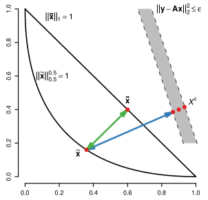
We can see that the solutions in the same 𝒳ϵsuperscript𝒳italic-ϵ\mathcal{X}^{\epsilon} all have the same entropy function value. Combining Proposition 4 and Proposition 2, we have 𝒳ϵ𝒙¨isuperscript𝒳italic-ϵsubscript¨𝒙𝑖\mathcal{X}^{\epsilon}\longleftrightarrow\ddot{{\bm{x}}}_{i}, as illustrated in Fig. 3.

Refer to caption
Figure 3: The one-to-one mapping in the noisy case: 𝒳ϵ𝒙~𝒙¨superscript𝒳italic-ϵ~𝒙¨𝒙\mathcal{X}^{\epsilon}\longleftrightarrow\tilde{{\bm{x}}}\longleftrightarrow\ddot{{\bm{x}}} when p=0.5𝑝0.5p=0.5.

Let 𝒳𝒳\mathcal{X} be the set defined in Proposition 4. Specifically, 𝒳ϵ=𝒳1ϵ𝒳2ϵsuperscript𝒳italic-ϵsubscriptsuperscript𝒳italic-ϵ1subscriptsuperscript𝒳italic-ϵ2\mathcal{X}^{\epsilon}=\mathcal{X}^{\epsilon}_{1}\cup\mathcal{X}^{\epsilon}_{2} and 𝒳1ϵ𝒳2ϵ=subscriptsuperscript𝒳italic-ϵ1subscriptsuperscript𝒳italic-ϵ2\mathcal{X}^{\epsilon}_{1}\cap\mathcal{X}^{\epsilon}_{2}=\emptyset, where 𝒳1ϵsubscriptsuperscript𝒳italic-ϵ1\mathcal{X}^{\epsilon}_{1} contains solutions on the boundary of the orthant 𝕆𝕆\mathbb{O}, and 𝒳2ϵsubscriptsuperscript𝒳italic-ϵ2\mathcal{X}^{\epsilon}_{2} contains the rest solutions that are not on the boundary. The solution 𝒙𝒙{\bm{x}} is then mapped to 𝒙¨¨𝒙\ddot{{\bm{x}}} one by one, producing the corresponding sets 𝒳¨1,𝒳¨2subscript¨𝒳1subscript¨𝒳2\ddot{\mathcal{X}}_{1},\ddot{\mathcal{X}}_{2} on the simplex x¨1=1subscriptnorm¨𝑥11\|\ddot{x}\|_{1}=1. Similarly we have:

Proposition 5.

In the noisy case where 𝐲𝐀𝐱22ϵsuperscriptsubscriptnorm𝐲𝐀𝐱22italic-ϵ\|{\bm{y}}-{\bm{A}}{\bm{x}}\|_{2}^{2}\leq\epsilon, for every solution 𝐱𝒳2ϵ𝐱subscriptsuperscript𝒳italic-ϵ2{\bm{x}}\in\mathcal{X}^{\epsilon}_{2}, there is a solution 𝐱𝒳1ϵsuperscript𝐱subscriptsuperscript𝒳italic-ϵ1{\bm{x}}^{*}\in\mathcal{X}^{\epsilon}_{1} on the boundary of the orthant 𝕆𝕆\mathbb{O} such that hp(𝐱)<hp(𝐱)subscript𝑝superscript𝐱subscript𝑝𝐱h_{p}({\bm{x}}^{*})<h_{p}({\bm{x}}) and hp,α(𝐱)<hp,α(𝐱)subscript𝑝𝛼superscript𝐱subscript𝑝𝛼𝐱h_{p,\alpha}({\bm{x}}^{*})<h_{p,\alpha}({\bm{x}}).

Proof.

From proposition 3, we have that for every 𝒙¨𝒳¨2¨𝒙subscript¨𝒳2\ddot{{\bm{x}}}\in\ddot{\mathcal{X}}_{2}, there is a 𝒙¨𝒳¨1superscript¨𝒙subscript¨𝒳1\ddot{{\bm{x}}}^{*}\in\ddot{\mathcal{X}}_{1} such that g(𝒙¨)<g(𝒙¨)𝑔superscript¨𝒙𝑔¨𝒙g(\ddot{{\bm{x}}}^{*})<g(\ddot{{\bm{x}}}).

Proposition 4 and 2 guarantee a one to one mapping in 𝕆𝕆\mathbb{O} between 𝒳ϵsuperscript𝒳italic-ϵ\mathcal{X}^{\epsilon} and 𝒙¨¨𝒙\ddot{{\bm{x}}}: 𝒳ϵ𝒙¨superscript𝒳italic-ϵ¨𝒙\mathcal{X}^{\epsilon}\longleftrightarrow\ddot{{\bm{x}}}. Since hp(𝒙)=g(𝒙¨)subscript𝑝𝒙𝑔¨𝒙h_{p}({\bm{x}})=g(\ddot{{\bm{x}}}) and hp,α(𝒙)=gα(𝒙¨)subscript𝑝𝛼𝒙subscript𝑔𝛼¨𝒙h_{p,\alpha}({\bm{x}})=g_{\alpha}(\ddot{{\bm{x}}}), for every 𝒙𝒳2ϵ𝒙subscriptsuperscript𝒳italic-ϵ2{\bm{x}}\in\mathcal{X}^{\epsilon}_{2}, there is an 𝒙𝒳1ϵsuperscript𝒙subscriptsuperscript𝒳italic-ϵ1{\bm{x}}^{*}\in\mathcal{X}^{\epsilon}_{1} such that hp(𝒙)<hp(𝒙)subscript𝑝superscript𝒙subscript𝑝𝒙h_{p}({\bm{x}}^{*})<h_{p}({\bm{x}}) and hp,α(𝒙)<hp,α(𝒙)subscript𝑝𝛼superscript𝒙subscript𝑝𝛼𝒙h_{p,\alpha}({\bm{x}}^{*})<h_{p,\alpha}({\bm{x}}). ∎

We can see that minimizing hp(𝒙)subscript𝑝𝒙h_{p}({\bm{x}}) or hp,α(𝒙)subscript𝑝𝛼𝒙h_{p,\alpha}({\bm{x}}) in the orthant 𝕆𝕆\mathbb{O} also leads to sparser solutions in 𝒳1ϵsubscriptsuperscript𝒳italic-ϵ1\mathcal{X}^{\epsilon}_{1} in the noisy case.

  • ❑ Local minimums:

    Here we formally introduce the following Proposition 6 on the local minimums of the generalized entropy functions:
    Refer to caption
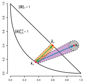
    Figure 4: The one-to-one mapping: ρ(𝒙o)ρ(𝒙~o)ρ(𝒙¨o)𝜌subscript𝒙𝑜𝜌subscript~𝒙𝑜𝜌subscript¨𝒙𝑜\rho({\bm{x}}_{o})\longleftrightarrow\rho(\tilde{{\bm{x}}}_{o})\longleftrightarrow\rho(\ddot{{\bm{x}}}_{o}) when p=0.5𝑝0.5p=0.5.
Proposition 6.

The local minimums of the generalized entropy functions hp(𝐱)subscript𝑝𝐱h_{p}({\bm{x}}) and hp,α(𝐱)subscript𝑝𝛼𝐱h_{p,\alpha}({\bm{x}}) only occur at the boundaries of each orthant in Nsuperscript𝑁\mathbb{R}^{N}.

Proof.

Without loss of generality, suppose 𝒙oNsubscript𝒙𝑜superscript𝑁{\bm{x}}_{o}\in\mathbb{R}^{N} is a local minimum of the generalized entropy function inside some orthant 𝕆𝕆\mathbb{O}, as illustrated in Fig. 4. There exists a small neighborhood ρ(𝒙o)𝜌subscript𝒙𝑜\rho({\bm{x}}_{o}) surrounding 𝒙osubscript𝒙𝑜{\bm{x}}_{o} such that 𝒙ρ(𝒙o)for-all𝒙𝜌subscript𝒙𝑜\forall{\bm{x}}\in\rho({\bm{x}}_{o}), hp(𝒙)hp(𝒙o)subscript𝑝𝒙subscript𝑝subscript𝒙𝑜h_{p}({\bm{x}})\geq h_{p}({\bm{x}}_{o}) or hp,α(𝒙)hp,α(𝒙o)subscript𝑝𝛼𝒙subscript𝑝𝛼subscript𝒙𝑜h_{p,\alpha}({\bm{x}})\geq h_{p,\alpha}({\bm{x}}_{o}).

As done in Proposition 1 and 4, we project 𝒙osubscript𝒙𝑜{\bm{x}}_{o} along with its neighborhood ρ(𝒙o)𝜌subscript𝒙𝑜\rho({\bm{x}}_{o}) respectively to 𝒙~osubscript~𝒙𝑜\tilde{{\bm{x}}}_{o} and ρ(𝒙~o)𝜌subscript~𝒙𝑜\rho(\tilde{{\bm{x}}}_{o}) on the sphere 𝒙~pp=1superscriptsubscriptnorm~𝒙𝑝𝑝1\|\tilde{{\bm{x}}}\|_{p}^{p}=1 inside the same orthant 𝕆𝕆\mathbb{O}:

𝒙o𝒙~oandρ(𝒙o)ρ(𝒙~o).subscript𝒙𝑜subscript~𝒙𝑜and𝜌subscript𝒙𝑜𝜌subscript~𝒙𝑜\displaystyle{\bm{x}}_{o}\longleftrightarrow\tilde{{\bm{x}}}_{o}\quad\textnormal{and}\quad\rho({\bm{x}}_{o})\longleftrightarrow\rho(\tilde{{\bm{x}}}_{o})\,. (22)

𝒙~osubscript~𝒙𝑜\tilde{{\bm{x}}}_{o} and ρ(𝒙~o)𝜌subscript~𝒙𝑜\rho(\tilde{{\bm{x}}}_{o}) are further projected to 𝒙¨osubscript¨𝒙𝑜\ddot{{\bm{x}}}_{o} and ρ(𝒙¨o)𝜌subscript¨𝒙𝑜\rho(\ddot{{\bm{x}}}_{o}) on the simplex 𝒙¨1=1subscriptnorm¨𝒙11\|\ddot{{\bm{x}}}\|_{1}=1 inside the same orthant 𝕆𝕆\mathbb{O}.

𝒙~o𝒙¨oandρ(𝒙~o)ρ(𝒙¨o).subscript~𝒙𝑜subscript¨𝒙𝑜and𝜌subscript~𝒙𝑜𝜌subscript¨𝒙𝑜\displaystyle\tilde{{\bm{x}}}_{o}\longleftrightarrow\ddot{{\bm{x}}}_{o}\quad\textnormal{and}\quad\rho(\tilde{{\bm{x}}}_{o})\longleftrightarrow\rho(\ddot{{\bm{x}}}_{o})\,. (23)

Consequently, 𝒙¨ρ(𝒙¨o)for-all¨𝒙𝜌subscript¨𝒙𝑜\forall\ddot{{\bm{x}}}\in\rho(\ddot{{\bm{x}}}_{o}), we have hp(𝒙¨)hp(𝒙¨o)subscript𝑝¨𝒙subscript𝑝subscript¨𝒙𝑜h_{p}(\ddot{{\bm{x}}})\geq h_{p}(\ddot{{\bm{x}}}_{o}) or hp,α(𝒙¨)hp,α(𝒙¨o)subscript𝑝𝛼¨𝒙subscript𝑝𝛼subscript¨𝒙𝑜h_{p,\alpha}(\ddot{{\bm{x}}})\geq h_{p,\alpha}(\ddot{{\bm{x}}}_{o}). 𝒙¨osubscript¨𝒙𝑜\ddot{{\bm{x}}}_{o} is also a corresponding local minimum 𝒙¨osubscript¨𝒙𝑜\ddot{{\bm{x}}}_{o} on the simplex 𝒙¨1=1subscriptnorm¨𝒙11\|\ddot{{\bm{x}}}\|_{1}=1 inside the orthant 𝕆𝕆\mathbb{O}.

However, we can show that such a local minimum 𝒙¨osubscript¨𝒙𝑜\ddot{{\bm{x}}}_{o} does not exist on the simplex 𝒙¨1=1subscriptnorm¨𝒙11\|\ddot{{\bm{x}}}\|_{1}=1 inside the orthant 𝕆𝕆\mathbb{O}:

  1. 1.

    SEF hp(𝒙¨)subscript𝑝¨𝒙h_{p}(\ddot{{\bm{x}}}) with p>0𝑝0p>0: It is strictly concave with respect to 𝒙¨¨𝒙\ddot{{\bm{x}}}, there are no local minimums on the simplex 𝒙¨1=1subscriptnorm¨𝒙11\|\ddot{{\bm{x}}}\|_{1}=1 inside the orthant 𝕆𝕆\mathbb{O}, i.e. 𝒙¨osubscript¨𝒙𝑜\ddot{{\bm{x}}}_{o} does not exist.

  2. 2.

    REF hp,α(𝒙¨)subscript𝑝𝛼¨𝒙h_{p,\alpha}(\ddot{{\bm{x}}}) with p>0𝑝0p>0, α>0𝛼0\alpha>0 and α1𝛼1\alpha\neq 1: When α(0,1)𝛼01\alpha\in(0,1), hp,α(𝒙¨)subscript𝑝𝛼¨𝒙h_{p,\alpha}(\ddot{{\bm{x}}}) is strictly concave with respect to 𝒙¨¨𝒙\ddot{{\bm{x}}}. When α(1,)𝛼1\alpha\in(1,\infty), hp,α(𝒙¨)subscript𝑝𝛼¨𝒙h_{p,\alpha}(\ddot{{\bm{x}}}) is strictly Schur concave with respect to 𝒙¨¨𝒙\ddot{{\bm{x}}} [56]. Hence 𝒙¨osubscript¨𝒙𝑜\ddot{{\bm{x}}}_{o} does not exist either.

We can see that there are no local minimums inside each orthant 𝕆𝕆\mathbb{O}. Furthermore, the local minimums of hp(𝒙¨)subscript𝑝¨𝒙h_{p}(\ddot{{\bm{x}}}) and hp,α(𝒙¨)subscript𝑝𝛼¨𝒙h_{p,\alpha}(\ddot{{\bm{x}}}) occur at the boundaries of the simplex 𝒙¨1=1subscriptnorm¨𝒙11\|\ddot{{\bm{x}}}\|_{1}=1. Hence the local minimums of hp(𝒙)subscript𝑝𝒙h_{p}({\bm{x}}) and hp,α(𝒙)subscript𝑝𝛼𝒙h_{p,\alpha}({\bm{x}}) also only occur at the boundary of each orthant 𝕆𝕆\mathbb{O}. ∎

II-D Energy-promoting Analysis

The sparsity-promoting property of the various regularizers already encourages the energy of the signal 𝒙22superscriptsubscriptnorm𝒙22\|{\bm{x}}\|_{2}^{2} to be concentrated in a few significant coefficients. Here we can show that minimizing the generalized entropy functions hp(𝒙)subscript𝑝𝒙h_{p}({\bm{x}}) and hp,α(𝒙)subscript𝑝𝛼𝒙h_{p,\alpha}({\bm{x}}) further promotes multiple high-energy coefficients while suppressing the rest low-energy coefficients within the recovered solution.

  • ❑ SEF:

    The energy-promoting property can be best illustrated from an optimization perspective. Take the SEF hp(𝒙)subscript𝑝𝒙h_{p}({\bm{x}}) for example, should we use the subderivative descent to minimize it, the solution 𝒙𝒙{\bm{x}} is updated as follows:

    𝒙=𝒙ηhp(𝒙)=𝒙ηsign(𝒙)hp(|𝒙|),𝒙𝒙𝜂subscript𝑝𝒙𝒙𝜂sign𝒙subscript𝑝𝒙\displaystyle\begin{split}{\bm{x}}&={\bm{x}}-\eta\cdot\partial h_{p}({\bm{x}})\\ &={\bm{x}}-\eta\cdot\textnormal{sign}({\bm{x}})\circ\nabla h_{p}(|{\bm{x}}|)\,,\end{split} (24)

    where η>0𝜂0\eta>0 is some suitable step size, and hp(|𝒙|)subscript𝑝𝒙\nabla h_{p}(|{\bm{x}}|) is the gradient with respect to the magnitude |𝒙|𝒙|{\bm{x}}|:

    hp(𝒙)|xi|=|xi|(i=1N|xi|plog|xi|p𝒙pp+log𝒙pp)=1𝒙pp(p|xi|p1log|xi|p+p|xi|p1)+p|xi|(p1)l=1N|xl|plog|xl|p𝒙p2p+p|xi|p1𝒙pp=p|xi|(p1)log|xi|p𝒙pp+p|xi|(p1)l=1N|xl|plog|xl|p𝒙p2p.subscript𝑝𝒙subscript𝑥𝑖subscript𝑥𝑖superscriptsubscript𝑖1𝑁superscriptsubscript𝑥𝑖𝑝superscriptsubscript𝑥𝑖𝑝superscriptsubscriptnorm𝒙𝑝𝑝superscriptsubscriptdelimited-∥∥𝒙𝑝𝑝1superscriptsubscriptnorm𝒙𝑝𝑝𝑝superscriptsubscript𝑥𝑖𝑝1superscriptsubscript𝑥𝑖𝑝𝑝superscriptsubscript𝑥𝑖𝑝1𝑝superscriptsubscript𝑥𝑖𝑝1superscriptsubscript𝑙1𝑁superscriptsubscript𝑥𝑙𝑝superscriptsubscript𝑥𝑙𝑝superscriptsubscriptnorm𝒙𝑝2𝑝𝑝superscriptsubscript𝑥𝑖𝑝1superscriptsubscriptnorm𝒙𝑝𝑝𝑝superscriptsubscript𝑥𝑖𝑝1superscriptsubscript𝑥𝑖𝑝subscriptsuperscriptnorm𝒙𝑝𝑝𝑝superscriptsubscript𝑥𝑖𝑝1superscriptsubscript𝑙1𝑁superscriptsubscript𝑥𝑙𝑝superscriptsubscript𝑥𝑙𝑝superscriptsubscriptnorm𝒙𝑝2𝑝\displaystyle\begin{split}&\frac{\partial h_{p}({\bm{x}})}{\partial|x_{i}|}=\frac{\partial}{\partial|x_{i}|}\left(-\frac{\sum_{i=1}^{N}|x_{i}|^{p}\log|x_{i}|^{p}}{\|{\bm{x}}\|_{p}^{p}}+\log\|{\bm{x}}\|_{p}^{p}\right)\\ &=-\frac{1}{\|{\bm{x}}\|_{p}^{p}}\left(p|x_{i}|^{p-1}\log|x_{i}|^{p}+p|x_{i}|^{p-1}\right)\\ &\quad+\frac{p|x_{i}|^{(p-1)}\sum_{l=1}^{N}|x_{l}|^{p}\log|x_{l}|^{p}}{\|{\bm{x}}\|_{p}^{2p}}+\frac{p|x_{i}|^{p-1}}{\|{\bm{x}}\|_{p}^{p}}\\ &=-\frac{p|x_{i}|^{(p-1)}\log|x_{i}|^{p}}{\|{\bm{x}}\|^{p}_{p}}+\frac{p|x_{i}|^{(p-1)}\sum_{l=1}^{N}|x_{l}|^{p}\log|x_{l}|^{p}}{\|{\bm{x}}\|_{p}^{2p}}.\end{split} (25)

    It’s easy to verify the following remark:

    Remark.

    Let ν=exp(l|xl|plog|xl|pp𝐱pp),ν>0formulae-sequence𝜈subscript𝑙superscriptsubscript𝑥𝑙𝑝superscriptsubscript𝑥𝑙𝑝𝑝superscriptsubscriptnorm𝐱𝑝𝑝𝜈0\nu=\exp\left(\frac{\sum_{l}|x_{l}|^{p}\log|x_{l}|^{p}}{p\|{\bm{x}}\|_{p}^{p}}\right),\nu>0, we have:

    hp(𝒙)|xi|{<0=0>0if |xi|>νif |xi|=νif |xi|<ν.subscript𝑝𝒙subscript𝑥𝑖casesabsent0absent0absent0if |xi|>νif |xi|=νif |xi|<ν\displaystyle\frac{\partial h_{p}({\bm{x}})}{\partial|x_{i}|}\left\{\begin{array}[]{l}<0\\ =0\\ >0\end{array}\quad\begin{array}[]{l}\textnormal{if $|x_{i}|>\nu$}\\ \textnormal{if $|x_{i}|=\nu$}\\ \textnormal{if $|x_{i}|<\nu$}\,.\end{array}\right. (32)
Refer to caption
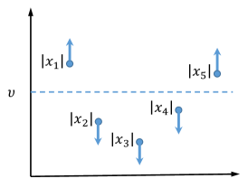
Figure 5: When the magnitude of the i𝑖i-th entry |xi|>νsubscript𝑥𝑖𝜈|x_{i}|>\nu, the update in (24) makes |xi|subscript𝑥𝑖|x_{i}| larger. When |xi|<νsubscript𝑥𝑖𝜈|x_{i}|<\nu, the update in (24) makes |xi|subscript𝑥𝑖|x_{i}| smaller.

As illustrated in Fig. 5, for the entries with relatively large magnitudes |xi|>νsubscript𝑥𝑖𝜈|x_{i}|>\nu, we can see that the update in (24) makes their magnitudes even larger. Conversely, if the entries have relatively small magnitudes |xi|<νsubscript𝑥𝑖𝜈|x_{i}|<\nu, the update makes their magnitudes even smaller. In this way minimizing hp(𝒙)subscript𝑝𝒙h_{p}({\bm{x}}) promotes large-magnitude entries while suppressing small-magnitude entries in the recovered signal.

  • ❑ REF:

    For the REF hp,α(𝒙)subscript𝑝𝛼𝒙h_{p,\alpha}({\bm{x}}), the derivative with respect to the magnitude |𝒙|𝒙|{\bm{x}}| is:

    hp,α(𝒙)|xi|=11α×1l=1N(|xl|𝒙p)pα×pα𝒙pp(α+1)×[|xi|pα1𝒙pp|xi|p1𝒙pαpα].\displaystyle\begin{split}\frac{\partial h_{p,\alpha}({\bm{x}})}{\partial|x_{i}|}&=\frac{1}{1-\alpha}\times\frac{1}{\sum_{l=1}^{N}\left(\frac{|x_{l}|}{\|{\bm{x}}\|_{p}}\right)^{p\alpha}}\times\frac{p\alpha}{\|{\bm{x}}\|_{p}^{p(\alpha+1)}}\\ &\quad\quad\times\left[|x_{i}|^{p\alpha-1}\|{\bm{x}}\|_{p}^{p}-|x_{i}|^{p-1}\|{\bm{x}}\|_{p\alpha}^{p\alpha}\right]\,.\end{split} (33)

    Similarly we have the following remark:

    Remark.

    Let ν=exp(1pαplog𝐱pαpα𝐱pp),ν>0formulae-sequence𝜈1𝑝𝛼𝑝superscriptsubscriptnorm𝐱𝑝𝛼𝑝𝛼superscriptsubscriptnorm𝐱𝑝𝑝𝜈0\nu=\exp\left(\frac{1}{p\alpha-p}\log\frac{\|{\bm{x}}\|_{p\alpha}^{p\alpha}}{\|{\bm{x}}\|_{p}^{p}}\right),\nu>0, we have:

    hp,α(𝒙)|xi|{<0=0>0if |xi|>νif |xi|=νif |xi|<ν.subscript𝑝𝛼𝒙subscript𝑥𝑖casesabsent0absent0absent0if |xi|>νif |xi|=νif |xi|<ν\displaystyle\frac{\partial h_{p,\alpha}({\bm{x}})}{\partial|x_{i}|}\left\{\begin{array}[]{l}<0\\ =0\\ >0\end{array}\quad\begin{array}[]{l}\textnormal{if $|x_{i}|>\nu$}\\ \textnormal{if $|x_{i}|=\nu$}\\ \textnormal{if $|x_{i}|<\nu$}\,.\end{array}\right. (40)

    We can see that minimizing hp,α(𝒙)subscript𝑝𝛼𝒙h_{p,\alpha}({\bm{x}}) also promotes large-magnitude entries while suppressing small-magnitude entries in the recovered signal.

As discussed in Appendix B, we can see that minimizing the other regularizers introduced in section I-A1 do not have such energy-promoting behaviors.

II-D1 Advantage in SRC

This energy-promoting behavior becomes handy in applications such as sparse representation classification (SRC) [58, 59]. Specifically, suppose the subspace of interest is spanned by the columns of 𝑨=[𝑨1𝑨2𝑨C𝑰]𝑨delimited-[]subscript𝑨1subscript𝑨2subscript𝑨𝐶𝑰{\bm{A}}=[{\bm{A}}_{1}\,{\bm{A}}_{2}\cdots{\bm{A}}_{C}\,{\bm{I}}], where 𝑨isubscript𝑨𝑖{\bm{A}}_{i} is a block matrix whose columns are the collected samples belonging to the i𝑖i-th class, and 𝑰𝑰{\bm{I}} is the identity matrix used as the dictionary for the noise. The 𝒙𝒙{\bm{x}} can be written accordingly as 𝒙T=[𝒙1T𝒙2T𝒙CT𝒙𝑰T]superscript𝒙Tdelimited-[]superscriptsubscript𝒙1Tsuperscriptsubscript𝒙2Tsuperscriptsubscript𝒙𝐶Tsuperscriptsubscript𝒙𝑰T{\bm{x}}^{\textnormal{T}}=[{\bm{x}}_{1}^{\textnormal{T}}\,\,{\bm{x}}_{2}^{\textnormal{T}}\,\,\cdots{\bm{x}}_{C}^{\textnormal{T}}\,\,{\bm{x}}_{{\bm{I}}}^{\textnormal{T}}], where 𝒙isubscript𝒙𝑖{\bm{x}}_{i} contains the coefficients corresponding to the i𝑖i-th class, and 𝒙𝑰subscript𝒙𝑰{\bm{x}}_{{\bm{I}}} is the noise. Additionally, we assume the block matrix 𝑨isubscript𝑨𝑖{\bm{A}}_{i} satisfies the following restricted isometry property for some δ(i)(0,1)𝛿𝑖01\delta(i)\in(0,1) [7]:

1δ(i)𝒙i2𝑨i𝒙i21+δ(i)𝒙i2.1𝛿𝑖subscriptnormsubscript𝒙𝑖2subscriptnormsubscript𝑨𝑖subscript𝒙𝑖21𝛿𝑖subscriptnormsubscript𝒙𝑖2\displaystyle\sqrt{1-\delta(i)}\|{\bm{x}}_{i}\|_{2}\leq\|{\bm{A}}_{i}{\bm{x}}_{i}\|_{2}\leq\sqrt{1+\delta(i)}\|{\bm{x}}_{i}\|_{2}\,. (41)

After the solution 𝒙𝒙{\bm{x}} that satisfies the constraint 𝒚𝑨𝒙2ϵsubscriptnorm𝒚𝑨𝒙2italic-ϵ\|{\bm{y}}-{\bm{A}}{\bm{x}}\|_{2}\leq\sqrt{\epsilon} is computed, the following residues are computed for every class:

σi=𝒚𝒙𝑰𝑨i𝒙i2,i[1,,C].formulae-sequencesubscript𝜎𝑖subscriptnorm𝒚subscript𝒙𝑰subscript𝑨𝑖subscript𝒙𝑖2for-all𝑖1𝐶\displaystyle\sigma_{i}=\|{\bm{y}}-{\bm{x}}_{{\bm{I}}}-{\bm{A}}_{i}{\bm{x}}_{i}\|_{2},\quad\forall i\in[1,\cdots,C]\,. (42)

The class label of 𝒚𝒚{\bm{y}} is then:

c=argminiσi.𝑐subscript𝑖subscript𝜎𝑖\displaystyle c=\arg\textstyle\min_{i}\,\,\sigma_{i}\,. (43)

Without loss of generality, suppose 𝒚𝒚{\bm{y}} belongs to the 111st class, and we are comparing σ1subscript𝜎1\sigma_{1} and σ2subscript𝜎2\sigma_{2}. Let 𝑨1,2¯¯subscript𝑨12\overline{{\bm{A}}_{1,2}} denote the matrix obtained after removing 𝑨1subscript𝑨1{\bm{A}}_{1} and 𝑨2subscript𝑨2{\bm{A}}_{2} from 𝑨𝑨{\bm{A}}, while 𝒙1,2¯¯subscript𝒙12\overline{{\bm{x}}_{1,2}} denotes the vector obtained after removing 𝒙1subscript𝒙1{\bm{x}}_{1} and 𝒙2subscript𝒙2{\bm{x}}_{2} from 𝒙𝒙{\bm{x}}. We then have:

𝒚𝒙𝑰𝑨1𝒙1𝑨2𝒙2𝑨1,2¯𝒙1,2¯2ϵ.subscriptnorm𝒚subscript𝒙𝑰subscript𝑨1subscript𝒙1subscript𝑨2subscript𝒙2¯subscript𝑨12¯subscript𝒙122italic-ϵ\displaystyle\|{\bm{y}}-{\bm{x}}_{{\bm{I}}}-{\bm{A}}_{1}{\bm{x}}_{1}-{\bm{A}}_{2}{\bm{x}}_{2}-\overline{{\bm{A}}_{1,2}}\overline{{\bm{x}}_{1,2}}\|_{2}\leq\sqrt{\epsilon}\,. (44)

Using the reverse triangle inequality, we have:

𝒚𝒙𝑰𝑨1𝒙12𝑨2𝒙2+𝑨1,2¯𝒙1,2¯2ϵsubscriptnorm𝒚subscript𝒙𝑰subscript𝑨1subscript𝒙12subscriptnormsubscript𝑨2subscript𝒙2¯subscript𝑨12¯subscript𝒙122italic-ϵ\displaystyle\|{\bm{y}}-{\bm{x}}_{{\bm{I}}}-{\bm{A}}_{1}{\bm{x}}_{1}\|_{2}-\|{\bm{A}}_{2}{\bm{x}}_{2}+\overline{{\bm{A}}_{1,2}}\overline{{\bm{x}}_{1,2}}\|_{2}\leq\sqrt{\epsilon} (45)
σ1=𝒚𝒙𝑰𝑨1𝒙12𝑨2𝒙22+𝑨1,2¯𝒙1,2¯2+ϵ1+δ(2)𝒙22+i{1,2}1+δ(i)𝒙i2+ϵ.subscript𝜎1subscriptdelimited-∥∥𝒚subscript𝒙𝑰subscript𝑨1subscript𝒙12subscriptdelimited-∥∥subscript𝑨2subscript𝒙22subscriptdelimited-∥∥¯subscript𝑨12¯subscript𝒙122italic-ϵ1𝛿2subscriptdelimited-∥∥subscript𝒙22subscript𝑖121𝛿𝑖subscriptdelimited-∥∥subscript𝒙𝑖2italic-ϵ\displaystyle\begin{split}&\sigma_{1}=\|{\bm{y}}-{\bm{x}}_{{\bm{I}}}-{\bm{A}}_{1}{\bm{x}}_{1}\|_{2}\\ &\quad\leq\|{\bm{A}}_{2}{\bm{x}}_{2}\|_{2}+\|\overline{{\bm{A}}_{1,2}}\overline{{\bm{x}}_{1,2}}\|_{2}+\sqrt{\epsilon}\\ &\quad\leq\sqrt{1+\delta(2)}\|{\bm{x}}_{2}\|_{2}+\textstyle\sum_{i\neq\{1,2\}}\sqrt{1+\delta(i)}\|{\bm{x}}_{i}\|_{2}+\sqrt{\epsilon}\,.\end{split} (46)

Using the reverse triangle inequality, we have:

𝒚𝒙𝑰𝑨2𝒙22𝑨1𝒙1+𝑨1,2¯𝒙1,2¯2ϵsubscriptnorm𝒚subscript𝒙𝑰subscript𝑨2subscript𝒙22subscriptnormsubscript𝑨1subscript𝒙1¯subscript𝑨12¯subscript𝒙122italic-ϵ\displaystyle\|{\bm{y}}-{\bm{x}}_{{\bm{I}}}-{\bm{A}}_{2}{\bm{x}}_{2}\|_{2}-\|{\bm{A}}_{1}{\bm{x}}_{1}+\overline{{\bm{A}}_{1,2}}\overline{{\bm{x}}_{1,2}}\|_{2}\geq-\sqrt{\epsilon} (47)
σ2=𝒚𝒙𝑰𝑨2𝒙22𝑨1𝒙1+𝑨1,2¯𝒙1,2¯2ϵ𝑨1𝒙12𝑨1,2¯𝒙1,2¯2ϵ1δ(1)𝒙12i{1,2}1+δ(i)𝒙i2ϵ.subscript𝜎2subscriptdelimited-∥∥𝒚subscript𝒙𝑰subscript𝑨2subscript𝒙22subscriptdelimited-∥∥subscript𝑨1subscript𝒙1¯subscript𝑨12¯subscript𝒙122italic-ϵsubscriptdelimited-∥∥subscript𝑨1subscript𝒙12subscriptdelimited-∥∥¯subscript𝑨12¯subscript𝒙122italic-ϵ1𝛿1subscriptdelimited-∥∥subscript𝒙12subscript𝑖121𝛿𝑖subscriptdelimited-∥∥subscript𝒙𝑖2italic-ϵ\displaystyle\begin{split}&\sigma_{2}=\|{\bm{y}}-{\bm{x}}_{{\bm{I}}}-{\bm{A}}_{2}{\bm{x}}_{2}\|_{2}\\ &\quad\geq\|{\bm{A}}_{1}{\bm{x}}_{1}+\overline{{\bm{A}}_{1,2}}\overline{{\bm{x}}_{1,2}}\|_{2}-\sqrt{\epsilon}\\ &\quad\geq\|{\bm{A}}_{1}{\bm{x}}_{1}\|_{2}-\|\overline{{\bm{A}}_{1,2}}\overline{{\bm{x}}_{1,2}}\|_{2}-\sqrt{\epsilon}\\ &\quad\geq\sqrt{1-\delta(1)}\|{\bm{x}}_{1}\|_{2}-\textstyle\sum_{i\neq\{1,2\}}\sqrt{1+\delta(i)}\|{\bm{x}}_{i}\|_{2}-\sqrt{\epsilon}\,.\end{split} (48)

We can see that (46) gives an upper bound on σ1subscript𝜎1\sigma_{1}, and we would like to keep it small. Hence 𝒙i2subscriptnormsubscript𝒙𝑖2\|{\bm{x}}_{i}\|_{2}, i1for-all𝑖1\forall i\neq 1 should be small. While (48) gives a lower bound on σ2subscript𝜎2\sigma_{2}, and we would like to keep it large. Hence 𝒙12subscriptnormsubscript𝒙12\|{\bm{x}}_{1}\|_{2} should be large, while 𝒙inormsubscript𝒙𝑖\|{\bm{x}}_{i}\|, i{1,2}for-all𝑖12\forall i\neq\{1,2\} should be small. In other words, we would like to promote the energy of 𝒙1subscript𝒙1{\bm{x}}_{1} and suppress the energy of 𝒙isubscript𝒙𝑖{\bm{x}}_{i}, i1for-all𝑖1\forall i\neq 1 at the same time. The energy-promoting property of the generalized entropy functions is well suited for this purpose.

III Entropy Function Minimization

Here we present the algorithm to perform the sparse signal recovery tasks formalized in (13),(14). The data fidelity term f(𝒙)𝑓𝒙f({\bm{x}}) is convex and smooth, the sparsity regularizers hp(𝒙),hp,α(𝒙)subscript𝑝𝒙subscript𝑝𝛼𝒙h_{p}({\bm{x}}),h_{p,\alpha}({\bm{x}}) are nonconvex and nonsmooth. FISTA [43] is adapted as the accelerated inexact proximal gradient method [52] to minimize the nonconvex objective functions.

III-A Inexact Proximal Gradient Method

Using the generalized Shannon entropy function hp(𝒙)subscript𝑝𝒙h_{p}({\bm{x}}) as an example, we first introduce the inexact proximal gradient method to solve the nonconvex problem (13):

  • Step 1:

    Proximal regularization using the data fidelity term f(𝒙)=𝒚𝑨𝒙22𝑓𝒙superscriptsubscriptnorm𝒚𝑨𝒙22f({\bm{x}})=\|{\bm{y}}-{\bm{A}}{\bm{x}}\|_{2}^{2}.

    In the (t+1)𝑡1(t+1)-th iteration, we use the proximal regularization [50] of f(𝒙)𝑓𝒙f({\bm{x}}) at 𝒙(t)superscript𝒙𝑡{\bm{x}}^{(t)}, as done in [43]:

    f(𝒙)=𝒚𝑨𝒙22f(𝒙(t))+𝒙𝒙(t),f(𝒙(t))+κ2𝒙𝒙(t)22=o(𝒙(t))+κ2𝒙(𝒙(t)1κf(𝒙(t)))22,𝑓𝒙superscriptsubscriptdelimited-∥∥𝒚𝑨𝒙22𝑓superscript𝒙𝑡𝒙superscript𝒙𝑡𝑓superscript𝒙𝑡𝜅2superscriptsubscriptdelimited-∥∥𝒙superscript𝒙𝑡22𝑜superscript𝒙𝑡𝜅2superscriptsubscriptdelimited-∥∥𝒙superscript𝒙𝑡1𝜅𝑓superscript𝒙𝑡22\displaystyle\begin{split}f({\bm{x}})&=\|{\bm{y}}-{\bm{A}}{\bm{x}}\|_{2}^{2}\\ &\leq f({\bm{x}}^{(t)})+\left<{\bm{x}}-{\bm{x}}^{(t)},\nabla f({\bm{x}}^{(t)})\right>+\frac{\kappa}{2}\left\|{\bm{x}}-{\bm{x}}^{(t)}\right\|_{2}^{2}\\ &=o({\bm{x}}^{(t)})+\frac{\kappa}{2}\left\|{\bm{x}}-\left({\bm{x}}^{(t)}-\frac{1}{\kappa}\nabla f({\bm{x}}^{(t)})\right)\right\|_{2}^{2}\,,\end{split} (49)

    where o(𝒙(t))𝑜superscript𝒙𝑡o({\bm{x}}^{(t)}) is a relative constant depending on the previous t𝑡t-th iteration’s solution 𝒙(t)superscript𝒙𝑡{\bm{x}}^{(t)} and can thus be ignored; f(𝒙(t))=2(𝑨T𝑨𝒙(t)𝑨T𝒚)𝑓superscript𝒙𝑡2superscript𝑨T𝑨superscript𝒙𝑡superscript𝑨T𝒚\nabla f({\bm{x}}^{(t)})=2({\bm{A}}^{\textrm{T}}{\bm{A}}{\bm{x}}^{(t)}-{\bm{A}}^{\textrm{T}}{\bm{y}}); the κ𝜅\kappa is the Lipschitz constant of the gradient f(𝒙(t))𝑓superscript𝒙𝑡\nabla f({\bm{x}}^{(t)}) [60]. The smallest value κ𝜅\kappa can take is twice the largest eigenvalue of 𝑨T𝑨superscript𝑨T𝑨{\bm{A}}^{\textrm{T}}{\bm{A}}, this is to ensure that f(𝒙)𝑓𝒙f({\bm{x}}) in (49) is upper-bounded by the proximal regularization at the right-hand side. When κ𝜅\kappa is unknown or difficult to compute, we can use the backtracking strategy describe in [43] to find it.

    Plug (49) into (13), we need to solve the following proximal operator of the nonconvex function hp(𝒙)subscript𝑝𝒙h_{p}({\bm{x}}):

    proxλκhp(𝒙(t)1κf(𝒙(t)))=argmin𝒙Rp(𝒙)=argmin𝒙κ2𝒙(𝒙(t)1κf(𝒙(t)))22+λhp(𝒙).subscriptprox𝜆𝜅subscript𝑝superscript𝒙𝑡1𝜅𝑓superscript𝒙𝑡subscript𝒙subscript𝑅𝑝𝒙subscript𝒙𝜅2superscriptsubscriptdelimited-∥∥𝒙superscript𝒙𝑡1𝜅𝑓superscript𝒙𝑡22𝜆subscript𝑝𝒙\displaystyle\begin{split}&\textnormal{prox}_{\frac{\lambda}{\kappa}h_{p}}\left({\bm{x}}^{(t)}-\frac{1}{\kappa}\nabla f({\bm{x}}^{(t)})\right)=\arg\min_{{\bm{x}}}R_{p}({\bm{x}})\\ &=\arg\min_{{\bm{x}}}\frac{\kappa}{2}\left\|{\bm{x}}-\left({\bm{x}}^{(t)}-\frac{1}{\kappa}\nabla f({\bm{x}}^{(t)})\right)\right\|_{2}^{2}+\lambda\,\,h_{p}({\bm{x}})\,.\end{split} (50)
  • Step 2:

    The nonconvex proximal operator (50) is inexactly solved.

    Since (50) is nonconvex, it is still an open-problem to obtain closed-form or exact solution [52, 61, 62]. Our goal here is to approximately solve it so that the solution 𝒓𝒓{\bm{r}}:

    Rp(𝒓)subscript𝑅𝑝𝒓\displaystyle R_{p}({\bm{r}}) Rp(𝒙(t)).absentsubscript𝑅𝑝superscript𝒙𝑡\displaystyle\leq R_{p}({\bm{x}}^{(t)})\,. (51)

    As shown in Appendix A, this would ensure the solution converges to a critical point.

    The nonconvex function hp(𝒙)subscript𝑝𝒙h_{p}({\bm{x}}) is replaced with its first-order approximation:

    hp(𝒙)hp(|𝒙(t)|)+|𝒙||𝒙(t)|,hp(|𝒙(t)|),subscript𝑝𝒙subscript𝑝superscript𝒙𝑡𝒙superscript𝒙𝑡subscript𝑝superscript𝒙𝑡\displaystyle\begin{split}h_{p}({\bm{x}})&\approx h_{p}(|{\bm{x}}^{(t)}|)+\left<|{\bm{x}}|-|{\bm{x}}^{(t)}|,\nabla h_{p}(|{\bm{x}}^{(t)}|)\right>\,,\end{split} (52)

    where hp(|𝒙|)subscript𝑝𝒙\nabla h_{p}(|{\bm{x}}|) is the gradient with respect to the modulus |xi|subscript𝑥𝑖|x_{i}| given in (25). When computing hp(|xi(t)|)subscript𝑝superscriptsubscript𝑥𝑖𝑡\nabla h_{p}(|x_{i}^{(t)}|), we add a small positive value ϵ=1012italic-ϵsuperscript1012\epsilon=10^{-12} to |xi(t)|superscriptsubscript𝑥𝑖𝑡|x_{i}^{(t)}| to avoid log00\log 0. Ignoring the relative constant terms in (52) that depend only on 𝒙(t)superscript𝒙𝑡{\bm{x}}^{(t)}, the proximal operator (50) can be approximated:

    𝒓=argmin𝒙κ2𝒙𝒔(t)22+λ|𝒙|,hp(|𝒙(t)|),𝒓subscript𝒙𝜅2superscriptsubscriptdelimited-∥∥𝒙superscript𝒔𝑡22𝜆𝒙subscript𝑝superscript𝒙𝑡\displaystyle\begin{split}{\bm{r}}=\arg\min_{{\bm{x}}}\,&\frac{\kappa}{2}\left\|{\bm{x}}-{\bm{s}}^{(t)}\right\|_{2}^{2}+\lambda\left<|{\bm{x}}|,\nabla h_{p}(|{\bm{x}}^{(t)}|)\right>\,,\end{split} (53)

    where 𝒔(t)=𝒙(t)1κf(𝒙(t))superscript𝒔𝑡superscript𝒙𝑡1𝜅𝑓superscript𝒙𝑡{\bm{s}}^{(t)}={\bm{x}}^{(t)}-\frac{1}{\kappa}\nabla f({\bm{x}}^{(t)}). This is a simple reweighted l1subscript𝑙1l_{1}-norm minimization problem that consists of a series of independent one-dimensional problems. The solution risubscript𝑟𝑖r_{i} to (53) can be obtained using the soft shrinkage operator:

    risubscript𝑟𝑖\displaystyle r_{i} =Γλκhp(|xi(t)|)(si(t)),absentsubscriptΓ𝜆𝜅subscript𝑝superscriptsubscript𝑥𝑖𝑡superscriptsubscript𝑠𝑖𝑡\displaystyle=\Gamma_{\frac{\lambda}{\kappa}\nabla h_{p}(|x_{i}^{(t)}|)}\left(s_{i}^{(t)}\right)\,, (54)

    where Γτ()subscriptΓ𝜏\Gamma_{\tau}(\cdot) is defined as follows:

    Γτ(x)={0(|x|τ)sign(x)if |x|τif |x|>τ.subscriptΓ𝜏𝑥cases0𝑥𝜏sign𝑥if |x|τif |x|>τ\displaystyle\Gamma_{\tau}(x)=\left\{\begin{array}[]{l}0\\ (|x|-\tau)\cdot\textrm{sign}(x)\end{array}\quad\begin{array}[]{l}\textrm{if $|x|\leq\tau$}\\ \textrm{if $|x|>\tau$}\,.\end{array}\right. (59)

    Conventionally, the soft shrinkage operator solves a convex problem and requires the threshold τ𝜏\tau to be positive. However, the gradient hp(|𝒙(t)|)subscript𝑝superscript𝒙𝑡\nabla h_{p}(|{\bm{x}}^{(t)}|) could be negative, which makes (53) nonconvex. In Appendix C we show that the global optimal solution can still be obtained using the soft thresholding operator in (59), yet with a different derivation process.

    We further update 𝒓𝒓{\bm{r}} as follows to ensure (51) holds:

    𝒓=𝒙(t)if Rp(𝒓)>Rp(𝒙(t)).𝒓superscript𝒙𝑡if Rp(𝒓)>Rp(𝒙(t))\displaystyle{\bm{r}}={\bm{x}}^{(t)}\quad\textrm{if $R_{p}({\bm{r}})>R_{p}({\bm{x}}^{(t)})$}\,. (60)
Refer to caption
Refer to caption
Refer to caption
Refer to caption
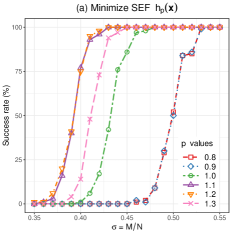
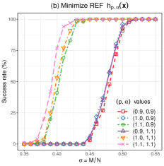
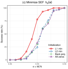
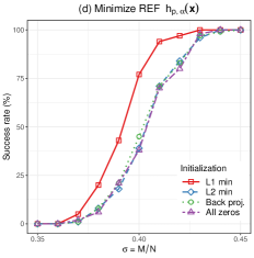
Figure 6: 6 and 6: the success rates of the recovery experiments with different parameter choices; 6 and 6 the success rates of the recovery experiments with different initialization strategies.

III-B Accelerated Inexact Proximal Gradient Method

The proximal gradient method [50, 51] was proposed to solve convex optimization problems, and the error from the optimum objective function is guaranteed to be within O(1t)𝑂1𝑡O(\frac{1}{t}) after t𝑡t iterations. Beck and Teboulle [43, 44] later proposed the accelerated proximal gradient method, a.k.a. FISTA, that has a convergence rate of O(1t2)𝑂1superscript𝑡2O(\frac{1}{t^{2}}). Li and Lin [52] later extended the accelerated proximal gradient (APG) to handle nonconvex and nonsmooth problems. In this case, the APG is guaranteed to converge to a critical point of the objective function [52]. Empirically, the APG could speed up the convergence by a great deal. However, it is still an open problem and a nontrival task to perform convergence rate analysis for general nonconvex objective functions [52, 61, 62].

Here we adapt the nonconvex acceleration approach by [52] to solve (13). Let Fp(𝒙)=f(𝒙)+λhp(𝒙)subscript𝐹𝑝𝒙𝑓𝒙𝜆subscript𝑝𝒙F_{p}({\bm{x}})=f({\bm{x}})+\lambda\,\,h_{p}({\bm{x}}), we have:

𝒖(t)=𝒙(t)+k(t1)k(t)(𝒛(t)𝒙(t))+k(t1)1k(t)(𝒙(t)𝒙(t1))superscript𝒖𝑡superscript𝒙𝑡superscript𝑘𝑡1superscript𝑘𝑡superscript𝒛𝑡superscript𝒙𝑡superscript𝑘𝑡11superscript𝑘𝑡superscript𝒙𝑡superscript𝒙𝑡1\displaystyle{\bm{u}}^{(t)}={\bm{x}}^{(t)}+\frac{k^{(t-1)}}{k^{(t)}}({\bm{z}}^{(t)}-{\bm{x}}^{(t)})+\frac{k^{(t-1)}-1}{k^{(t)}}({\bm{x}}^{(t)}-{\bm{x}}^{(t-1)}) (61)
𝒛(t+1)=proxλκhp(𝒖(t)1κf(𝒖(t)))superscript𝒛𝑡1subscriptprox𝜆𝜅subscript𝑝superscript𝒖𝑡1𝜅𝑓superscript𝒖𝑡\displaystyle{\bm{z}}^{(t+1)}=\textnormal{prox}_{\frac{\lambda}{\kappa}h_{p}}\left({\bm{u}}^{(t)}-\frac{1}{\kappa}\nabla f({\bm{u}}^{(t)})\right) (62)
𝒗(t+1)=proxλκhp(𝒙(t)1κf(𝒙(t)))superscript𝒗𝑡1subscriptprox𝜆𝜅subscript𝑝superscript𝒙𝑡1𝜅𝑓superscript𝒙𝑡\displaystyle{\bm{v}}^{(t+1)}=\textnormal{prox}_{\frac{\lambda}{\kappa}h_{p}}\left({\bm{x}}^{(t)}-\frac{1}{\kappa}\nabla f({\bm{x}}^{(t)})\right) (63)
k(t+1)=1+4(k(t))2+12superscript𝑘𝑡114superscriptsuperscript𝑘𝑡212\displaystyle k^{(t+1)}=\frac{1+\sqrt{4\left(k^{(t)}\right)^{2}+1}}{2} (64)
𝒙(t+1)={𝒛(t+1)𝒗(t+1)if Fp(𝒛(t+1))Fp(𝒗(t+1))otherwise.superscript𝒙𝑡1casessuperscript𝒛𝑡1superscript𝒗𝑡1if Fp(𝒛(t+1))Fp(𝒗(t+1))otherwise\displaystyle{\bm{x}}^{(t+1)}=\left\{\begin{array}[]{l}{\bm{z}}^{(t+1)}\\ {\bm{v}}^{(t+1)}\end{array}\quad\begin{array}[]{l}\textnormal{if $F_{p}({\bm{z}}^{(t+1)})\leq F_{p}({\bm{v}}^{(t+1)})$}\\ \textnormal{otherwise}\,.\end{array}\right. (69)

The iterations are stopped either when the maximum number of iterations is reached or when 𝒙(t+1)superscript𝒙𝑡1{\bm{x}}^{(t+1)} reaches convergence, i.e. 𝒙(t+1)𝒙(t)2𝒙(t+1)2τcsubscriptnormsuperscript𝒙𝑡1superscript𝒙𝑡2subscriptnormsuperscript𝒙𝑡12subscript𝜏𝑐\frac{\|{\bm{x}}^{(t+1)}-{\bm{x}}^{(t)}\|_{2}}{\|{\bm{x}}^{(t+1)}\|_{2}}\leq\tau_{c}. The convergence threshold τcsubscript𝜏𝑐\tau_{c} is usually chosen to be 0<τc1030subscript𝜏𝑐superscript1030<\tau_{c}\leq 10^{-3}.

Finally, the proposed entropy function minimization approach is summarized in Algorithm 1:

Algorithm 1 Sparse signal recovery via generalized entropy function minimization
1:{𝒚,𝑨},λ,κ,p,τc,T,k(1)=1,k(0)=0formulae-sequence𝒚𝑨𝜆𝜅𝑝subscript𝜏𝑐𝑇superscript𝑘11superscript𝑘00\{{\bm{y}},{\bm{A}}\},\lambda,\kappa,p,\tau_{c},T,k^{(1)}=1,k^{(0)}=0
2:Initialize 𝒙(0)superscript𝒙0{\bm{x}}^{(0)} with the solution from l1subscript𝑙1l_{1}-minimization;
3:Set 𝒛(1)=𝒙(1)=𝒙(0)superscript𝒛1superscript𝒙1superscript𝒙0{\bm{z}}^{(1)}={\bm{x}}^{(1)}={\bm{x}}^{(0)};
4:for t={1,,T}𝑡1𝑇t=\{1,\cdots,T\} do
5:   Update 𝒖𝒖{\bm{u}}, 𝒛𝒛{\bm{z}}, 𝒗𝒗{\bm{v}}, k𝑘k, 𝒙𝒙{\bm{x}} as in (61)-(69);
6:   if 𝒙(t+1)𝒙(t)2𝒙(t+1)2τcsubscriptnormsuperscript𝒙𝑡1superscript𝒙𝑡2subscriptnormsuperscript𝒙𝑡12subscript𝜏𝑐\frac{\left\|{\bm{x}}^{(t+1)}-{\bm{x}}^{(t)}\right\|_{2}}{\|{\bm{x}}^{(t+1)}\|_{2}}\leq\tau_{c} then
7:      Set 𝒙^=𝒙(t+1)^𝒙superscript𝒙𝑡1\hat{{\bm{x}}}={\bm{x}}^{(t+1)} and break.
8:   end if
9:end for
10:Return Output 𝒙^^𝒙\hat{{\bm{x}}};

III-C Regularization Parameter

Naturally, choosing a proper regularization parameter λ𝜆\lambda is the key to the success of sparse signal recovery.

III-C1 Noiseless recovery

The solution can be obtained by solving a series of minimization problems characterized by a decreasing λ𝜆\lambda sequence: λ0𝜆0\lambda\rightarrow 0 [49]. Take the Shannon entropy function hp(𝒙)subscript𝑝𝒙h_{p}({\bm{x}}) for example, we have the following:

1:Start with a relatively large λ0subscript𝜆0\lambda_{0}, and set 𝒙λ0superscript𝒙subscript𝜆0{\bm{x}}^{\lambda_{0}} to the l1subscript𝑙1l_{1}-minimization solution.
2:for l={1,,T}𝑙1𝑇l=\{1,\cdots,T\} do
3:   Use 𝒙λl1superscript𝒙subscript𝜆𝑙1{\bm{x}}^{\lambda_{l-1}} as the initializer, solve the minimization problem characterized by λlsubscript𝜆𝑙\lambda_{l}:
𝒙λl=argmin𝒙𝒚𝑨𝒙22+λlhp(𝒙).superscript𝒙subscript𝜆𝑙subscript𝒙superscriptsubscriptnorm𝒚𝑨𝒙22subscript𝜆𝑙subscript𝑝𝒙\displaystyle{\bm{x}}^{\lambda_{l}}=\arg\min_{{\bm{x}}}\,\|{\bm{y}}-{\bm{A}}{\bm{x}}\|_{2}^{2}+\lambda_{l}\,\,h_{p}({\bm{x}})\,. (70)
4:   Update λl+1=ρλlsubscript𝜆𝑙1𝜌subscript𝜆𝑙\lambda_{l+1}=\rho\cdot\lambda_{l}.
5:   if 𝒙λl+1𝒙λl2𝒙λl+12τcsubscriptnormsuperscript𝒙subscript𝜆𝑙1superscript𝒙subscript𝜆𝑙2subscriptnormsuperscript𝒙subscript𝜆𝑙12subscript𝜏𝑐\frac{\left\|{\bm{x}}^{\lambda_{l+1}}-{\bm{x}}^{\lambda_{l}}\right\|_{2}}{\|{\bm{x}}^{\lambda_{l+1}}\|_{2}}\leq\tau_{c} then break.
6:end for

To ensure the best performance, ρ𝜌\rho is chosen in [0.9,1)0.91[0.9,1).

III-C2 Noisy recovery

The optimal λ𝜆\lambda depends on the noise level and is usually unknown. An optimal fixed λ𝜆\lambda can be pre-tuned on some development set and later used in practice.

III-D Constructing Suitable Entropy Functions

The choice of different p𝑝p and α𝛼\alpha values also greatly affects the recovery performance.

  • For the SEF hp(𝒙)subscript𝑝𝒙h_{p}({\bm{x}}), where p>0𝑝0p>0. The optimal p𝑝p value is usually around 111. In practice, we can focus on tuning p𝑝p in the range [0.8, 1.3]0.81.3[0.8,\,1.3].

  • For the REF hp,α(𝒙)subscript𝑝𝛼𝒙h_{p,\alpha}({\bm{x}}), where p>0𝑝0p>0 and 0<α10𝛼10<\alpha\neq 1. Both optimal p𝑝p and α𝛼\alpha values are usually around 111. Empirically, we can focus on tuning p𝑝p in the range [0.8, 1.3]0.81.3[0.8,\,1.3], and α𝛼\alpha in the range [0.9, 1)(1, 1.1]0.9111.1[0.9,\,1)\cup(1,\,1.1].

As an example, here we compare the noiseless recovery performances of different entropy functions. For the experiments, 100100100 random sparse signals 𝒙𝒙{\bm{x}} of length N=1000𝑁1000N=1000 and sparsity level S=200𝑆200S=200 are generated: the nonzero entries are independently and identically drawn from 𝒩(0,1)𝒩01\mathcal{N}(0,1). The sensing matrices 𝑨𝑨{\bm{A}}s are random Gaussian matrices with i.i.d entries following 𝒩(0,1)𝒩01\mathcal{N}(0,1), with the columns normalized and centralized. The number of measurements M𝑀M is varied in [350, 550]350550[350,\,550], and Algorithm 1 is used to obtain the recovered signal 𝒙^^𝒙\hat{{\bm{x}}}. The recovery is considered to be a success if 𝒙^𝒙2𝒙2<103subscriptnorm^𝒙𝒙2subscriptnorm𝒙2superscript103\frac{\|\hat{{\bm{x}}}-{\bm{x}}\|_{2}}{\|{\bm{x}}\|_{2}}<10^{-3}. The success rates out of the 100100100 recoveries for different choices of M,p,α𝑀𝑝𝛼M,p,\alpha are shown in Fig. 6.

III-E Initialization Strategy

A proper initialization is needed to ensure good performances for the nonconvex problems. Following the same experimental setup as section III-D, we choose p=1.1𝑝1.1p=1.1 for the SEF hp(𝒙)subscript𝑝𝒙h_{p}({\bm{x}}), and (p=1.1,α=1.1)formulae-sequence𝑝1.1𝛼1.1(p=1.1,\,\alpha=1.1) for the REF hp,α(𝒙)subscript𝑝𝛼𝒙h_{p,\alpha}({\bm{x}}). We compare the following initialization strategies:

  1. 1.

    The l1subscript𝑙1l_{1}-minimization solution.

  2. 2.

    The l2subscript𝑙2l_{2}-minimization solution, i.e. the Moore-Penrose pseudo-inverse of 𝒚𝒚{\bm{y}}: 𝑨T(𝑨𝑨T)1𝒚superscript𝑨Tsuperscript𝑨superscript𝑨T1𝒚{\bm{A}}^{\textnormal{T}}({\bm{A}}{\bm{A}}^{\textnormal{T}})^{-1}{\bm{y}}.

  3. 3.

    Back projection: 𝑨T𝒚superscript𝑨T𝒚{\bm{A}}^{\textnormal{T}}{\bm{y}}.

  4. 4.

    All zeros: [0,,0]Tsuperscript00T[0,\cdots,0]^{\textnormal{T}}.

The success rates using the above initializers are shown in Fig. 6. We can see that the solution from l1subscript𝑙1l_{1}-norm minimization usually leads to the best performances. It is thus used as the initializer in the proposed Algorithm 1.
Refer to caption
Refer to caption
Refer to caption
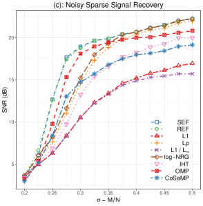
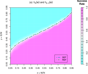
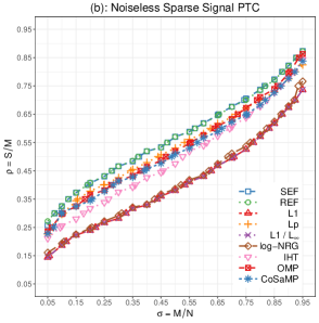
Figure 7: 7 The phase transition curves of hp(𝒙)subscript𝑝𝒙h_{p}({\bm{x}}) and hp,α(𝒙)subscript𝑝𝛼𝒙h_{p,\alpha}({\bm{x}}) divide the (ρ,σ)𝜌𝜎(\rho,\sigma) plane into the success phase and the failure phase; 7 The phase transition curves of different sparsity regularization approaches in the noiseless case; 7 The signal-to-noise-ratio (SNR) of the recovered signal 𝒙𝒙{\bm{x}} using different sparsity regularization approaches in the noisy case.

IV Experimental Results

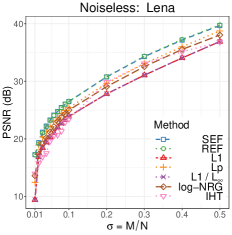
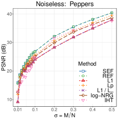
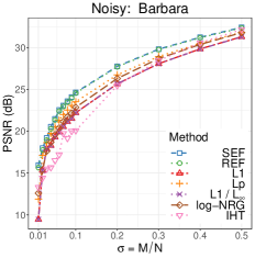
We compare the proposed Shannon entropy function (SEF) and Rényi entropy function (REF) regularizers with the relaxed sparsity-promoting regularizers introduced in section I-A1, OMP [12], CoSaMP [14] and the iterative hard thresholding (IHT) approach [10, 16, 17] that directly uses the 𝒙0subscriptnorm𝒙0\|{\bm{x}}\|_{0} as a regularizer on both simulated and real datasets.

The accelerated inexact proximal gradient method in Section III-B can be adapted to solve (6) when g(𝒙)𝑔𝒙g({\bm{x}}) is some other lower semi-continuous nonconvex/nonsmooth regularizers. The first-order approximation (52) needs to be updated accordingly. For best performances and a fair comparison, the l1subscript𝑙1l_{1}-minimization solution obtained via FISTA is used as the initializer for all the other approaches.

Take the regularizers introduced in section I-A1 for example, the function g3(𝒙)subscript𝑔3𝒙g_{3}({\bm{x}}) is a special case of g4(𝒙)subscript𝑔4𝒙g_{4}({\bm{x}}) for signals with fixed l1subscript𝑙1l_{1} norm; the functions g6(𝒙)subscript𝑔6𝒙g_{6}({\bm{x}}), \cdots, g9(𝒙)subscript𝑔9𝒙g_{9}({\bm{x}}) are special cases of the proposed entropy functions; the function g10(𝒙)subscript𝑔10𝒙g_{10}({\bm{x}}) is not a sparsity-promoting regularizer. For the experiments, we thus compare the proposed entropy functions with the rest regularizers.

Specifically, The l1subscript𝑙1l_{1} norm g1(𝒙)=𝒙1subscript𝑔1𝒙subscriptnorm𝒙1g_{1}({\bm{x}})=\|{\bm{x}}\|_{1} is minimized using FISTA. The lpsubscript𝑙𝑝l_{p} norm g2(𝒙)subscript𝑔2𝒙g_{2}({\bm{x}}) and the “L1/LsubscriptL1subscriptL\textnormal{L}_{1}/\textnormal{L}_{\infty}” function g4(𝒙)subscript𝑔4𝒙g_{4}({\bm{x}}) are minimized using Algorithm 1, i.e. adapted FISTA. We show that g2(𝒙)subscript𝑔2𝒙g_{2}({\bm{x}}), g4(𝒙)subscript𝑔4𝒙g_{4}({\bm{x}}) are both lower semi-continuous and give their first-order approximations in Appendix D. The “logarithm of energy” g5(𝒙)subscript𝑔5𝒙g_{5}({\bm{x}}) is not lower semi-continuous, its corresponding optimization problem is solved using the regularized FOCUSS algorithm [63, 64]: a reweighted l2subscript𝑙2l_{2} norm minimization algorithm.

The detailed experimental settings and code files can be found at https://github.com/shuai-huang/GEFM.
Refer to caption
Refer to caption
Refer to caption
Refer to caption
Refer to caption
Refer to caption
Refer to caption
Refer to caption
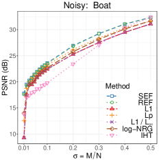
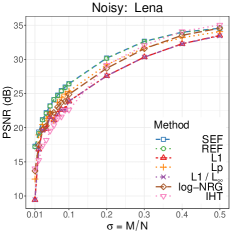
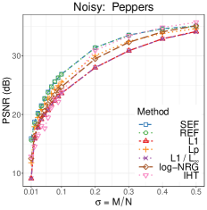
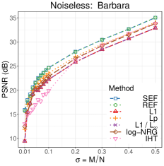
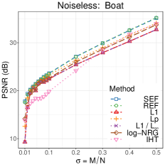
Figure 8: The PSNR of the recovered images using different sparsity regularization approaches.

IV-A Simulated Sparse Signal Recovery

IV-A1 Noiseless recovery

For the noiseless sparse signal recovery experiments, we fix N=1000𝑁1000N=1000 and vary the sampling ratio σ=MN[0.05,0.1,,0.95]𝜎𝑀𝑁0.050.10.95\sigma=\frac{M}{N}\in[0.05,0.1,\cdots,0.95] and the sparsity ratio ρ=SM[0.05,0.1,,0.95]𝜌𝑆𝑀0.050.10.95\rho=\frac{S}{M}\in[0.05,0.1,\cdots,0.95], where S𝑆S is the sparsity level of the signal, i.e. the number of nonzero coefficients. As mentioned in section I-A3, generally the sensing matrix 𝑨𝑨{\bm{A}} needs to satisfy the RIP to guarantee the uniqueness of the recovered solution 𝒙^^𝒙\hat{{\bm{x}}}. For each combination of σ𝜎\sigma and ρ𝜌\rho, we randomly generate 100100100 pairs of {𝒙,𝑨}𝒙𝑨\{{\bm{x}},{\bm{A}}\}: 𝑨𝑨{\bm{A}} is a M×N𝑀𝑁M\times N random Gaussian matrix with normalized and centralized columns. The nonzero entries of the sparse signal 𝒙N𝒙superscript𝑁{\bm{x}}\in\mathbb{R}^{N} are i.i.d. generated according to the Gaussian distribution 𝒩(0,1)𝒩01\mathcal{N}(0,1).

Given the measurement vector 𝒚=𝑨𝒙𝒚𝑨𝒙{\bm{y}}={\bm{A}}{\bm{x}} and the sensing matrix 𝑨𝑨{\bm{A}}, we try to recover the signal 𝒙𝒙{\bm{x}}. If ϵ=𝒙^𝒙2/𝒙2<103italic-ϵsubscriptnorm^𝒙𝒙2subscriptnorm𝒙2superscript103\epsilon=\|\hat{{\bm{x}}}-{\bm{x}}\|_{2}/\|{\bm{x}}\|_{2}<10^{-3}, the recovered 𝒙^^𝒙\hat{{\bm{x}}} is considered to be a success. A decreasing λ𝜆\lambda sequence was used to approach the optimal λ=0𝜆0\lambda=0 as explained in section III-C. The parameters were tuned to obtain best performance for each method: for the SEF minimization approach, p=1.1𝑝1.1p=1.1; for the REF minimization approach, p=1.1,α=1.1formulae-sequence𝑝1.1𝛼1.1p=1.1,\,\alpha=1.1; for the Lp minimization approach, p=0.5𝑝0.5p=0.5. The L1/LsubscriptL1subscriptL\textnormal{L}_{1}/\textnormal{L}_{\infty} function has a rigid energy-promoting behavior. When it is minimized, only the highest-energy coefficient(s) is/are promoted while the rest coefficients are suppressed. In our experiments, we found that the recovered 𝒙^^𝒙\hat{{\bm{x}}} generally converged to its initializer, i.e. the L1subscriptL1\textnormal{L}_{1}-min solution. For the log\log-energy minimization approach, as the lambda sequence went to 00, the regularized FOCUSS algorithm was equivalent to the original FOCUSS algorithm [64]. For the IHT approach, we scaled the sensing matrix 𝑨𝑨{\bm{A}} by its operator norm to make 𝑨2<1subscriptnorm𝑨21\|{\bm{A}}\|_{2}<1 as suggested by [10] to make the algorithm converge. For the OMP and CoSaMP, the sparsity level S𝑆S is tuned to obtain best performances. The measurement 𝒚𝒚{\bm{y}} was also scaled accordingly. Based on the 100100100 trials, we computed the success recovery rate for each combination of {σ,ρ}𝜎𝜌\{\sigma,\,\rho\}, and plotted the phase transition curves (PTC) in Fig. 7.

As shown in Fig. 7, the PTC is the contour that corresponds to the 0.5 success rate in the domain {σ,ρ}{0,1}2𝜎𝜌superscript012\{\sigma,\rho\}\in\{0,1\}^{2}, it divides the domain into a “success” phase (lower right) and a “failure” phase (upper left). We can see that the proposed SEF minimization and REF minimization approaches generally perform equally well, and they both perform better than the other approaches.

IV-A2 Noisy recovery

We next try to recover the sparse signal 𝒙𝒙{\bm{x}} from a noisy measurement vector 𝒚𝒚{\bm{y}}. Specifically, we fix S=100,N=1000formulae-sequence𝑆100𝑁1000S=100,N=1000 and increase M𝑀M gradually. The measurement 𝒚M𝒚superscript𝑀{\bm{y}}\in\mathbb{R}^{M} is generated as follows:

Noisy measurements:𝒚=𝑨𝒙+ν𝒘,Noisy measurements:𝒚𝑨𝒙𝜈𝒘\displaystyle\textrm{Noisy measurements:}\quad{\bm{y}}={\bm{A}}{\bm{x}}+\nu\cdot{\bm{w}}\,, (71)

where ν>0𝜈0\nu>0 controls the amount of noise added to 𝒚𝒚{\bm{y}}, the entries of 𝒘𝒘{\bm{w}} are i.i.d Gaussian 𝒩(0,1)𝒩01\mathcal{N}(0,1). We choose ν=0.05𝜈0.05\nu=0.05, this creates a measurement 𝒚𝒚{\bm{y}} with signal to noise ratio (SNR) around 252525 dB. We randomly generate 100100100 triples of {𝒙,𝑨,𝒘}𝒙𝑨𝒘\{{\bm{x}},{\bm{A}},{\bm{w}}\}. The average SNRs of the recovered signals 𝒙^^𝒙\hat{{\bm{x}}} are shown in Fig. 7. We can see that when σ<0.4𝜎0.4\sigma<0.4, the SEF and REF minimization approaches outperform the other approaches.

IV-B Real Image Recovery

Real images are considered to be approximately sparse under some proper basis, such as the DCT basis, wavelet basis, etc. Here we compare the recovery performances of the aforementioned sparsity regularization approaches based on varying noiseless and noisy measurements of the 444 real images shown in Fig. 9: Barbara, Boat, Lena, Peppers. Specifically, in order to reveal the sparse coefficients 𝒙𝒙{\bm{x}} of the real images 𝒔𝒔{\bm{s}}, we use the sparsity averaging method by [65] to construct an over-complete wavelet basis by concatenating Db1-Db4 [66]:

𝒔=Ψ(𝒙)=12i=14ΨDbi(𝒙),𝒔Ψ𝒙12superscriptsubscript𝑖14subscriptΨDb𝑖𝒙\displaystyle{\bm{s}}=\Psi({\bm{x}})=\frac{1}{2}\sum_{i=1}^{4}\Psi_{\textnormal{Db}i}({\bm{x}})\,, (72)

where ΨDbisubscriptΨDb𝑖\Psi_{\textnormal{Db}i} is the corresponding operator of the Dbi𝑖i wavelet. There is little performance improvement when adding more than 444 wavelet operators. The 1212\frac{1}{2} is introduced in (72) to ensure 𝒔=Ψ(𝒙)𝒔Ψ𝒙{\bm{s}}=\Psi({\bm{x}}), and 𝒙=Ψ(𝒔)𝒙superscriptΨ𝒔{\bm{x}}=\Psi^{\dagger}({\bm{s}}).

The sampling matrix 𝑼𝑼{\bm{U}} is constructed using the structurally random matrix approach by [67]: 𝑼=𝑫𝑭𝑹𝑼𝑫𝑭𝑹{\bm{U}}={\bm{D}}{\bm{F}}{\bm{R}}, where 𝑹𝑹{\bm{R}} is a uniform random permutation matrix that scrambles the signal’s sample locations globally while a diagonal matrix of Bernoulli random variables flips the signal’s sample signs locally, 𝑭𝑭{\bm{F}} is an orthonormal DCT matrix that computes fast transforms, 𝑫𝑫{\bm{D}} is a sub-sampling matrix that randomly selects a subset of the rows of the matrix 𝑭𝑹𝑭𝑹{\bm{F}}{\bm{R}}.

Refer to caption
Refer to caption
Refer to caption
Refer to caption
Figure 9: The real images used in the recovery experiments (from left to right): Barbara, Boat, Lena, Peppers.

The noiseless measurements 𝒚𝒚{\bm{y}} of the image 𝒔𝒔{\bm{s}} are obtained:

𝒚=𝑼𝒔.𝒚𝑼𝒔\displaystyle{\bm{y}}={\bm{U}}{\bm{s}}\,. (73)

The noisy measurements 𝒚𝒚{\bm{y}} are obtained:

𝒚=𝑼𝒔+ν𝒘.𝒚𝑼𝒔𝜈𝒘\displaystyle{\bm{y}}={\bm{U}}{\bm{s}}+\nu\cdot{\bm{w}}\,. (74)

The entries of the noise 𝒘𝒘{\bm{w}} are generated using i.i.d. Gaussian distribution 𝒩(0,1)𝒩01\mathcal{N}(0,1), ν𝜈\nu is chosen to be 0.020.020.02 so that the SNR of the measurement vector 𝒚𝒚{\bm{y}} is around 303030 dB444When ν𝜈\nu is set to other values, the relative performances of the four methods are similar..

Take the SEF minimization for example, the corresponding recovery problem is a cosparse problem [68] with respect to the image 𝒔𝒔{\bm{s}}:

min𝒔𝒚𝑼𝒔22+λhp(Ψ(𝒔)).subscript𝒔superscriptsubscriptnorm𝒚𝑼𝒔22𝜆subscript𝑝superscriptΨ𝒔\displaystyle\min_{{\bm{s}}}\,\|{\bm{y}}-{\bm{U}}{\bm{s}}\|_{2}^{2}+\lambda\,h_{p}\left(\Psi^{\dagger}({\bm{s}})\right)\,. (75)

The inexact proximal operator in the (t+1)𝑡1(t+1)-th iteration is:

proxλκhp(𝒔(t)2κ𝑼T(𝑼𝒔(t)𝒚))=argmin𝒔κ2𝒔(𝒔(t)2κ𝑼T(𝑼𝒔(t)𝒚))22+λhp(Ψ(𝒔)),subscriptprox𝜆𝜅subscript𝑝superscript𝒔𝑡2𝜅superscript𝑼T𝑼superscript𝒔𝑡𝒚subscript𝒔𝜅2superscriptsubscriptdelimited-∥∥𝒔superscript𝒔𝑡2𝜅superscript𝑼T𝑼superscript𝒔𝑡𝒚22𝜆subscript𝑝superscriptΨ𝒔\displaystyle\begin{split}&\textnormal{prox}_{\frac{\lambda}{\kappa}h_{p}}\left({\bm{s}}^{(t)}-\frac{2}{\kappa}\cdot{\bm{U}}^{\textrm{T}}({\bm{U}}{\bm{s}}^{(t)}-{\bm{y}})\right)\\ &=\arg\min_{{\bm{s}}}\,\frac{\kappa}{2}\left\|{\bm{s}}-\left({\bm{s}}^{(t)}-\frac{2}{\kappa}\cdot{\bm{U}}^{\textrm{T}}({\bm{U}}{\bm{s}}^{(t)}-{\bm{y}})\right)\right\|_{2}^{2}\\ &\quad\quad\quad\quad\quad+\lambda\,h_{p}\left(\Psi^{\dagger}({\bm{s}})\right),\end{split} (76)

where κ=2𝜅2\kappa=2 for the chosen sampling matrix 𝑼𝑼{\bm{U}}. The inexact proximal operator (76) can be efficiently solved using the alternating split bregman shrinkage algorithm by [69].

Since the real images are only approximately sparse, both the noiseless and noisy recovery experiments are performed using a fixed λ𝜆\lambda. The parameters were tuned to obtain best performance for each approach555Since no direct matrix-vector product form is available for 72, OMP and CoSaMP are not compared in the image recovery experiments.. For the SEF minimization approach, p=1𝑝1p=1, λ=5000𝜆5000\lambda=5000; for the REF minimization approach, p=0.9𝑝0.9p=0.9, α=1.1𝛼1.1\alpha=1.1, λ=104𝜆superscript104\lambda=10^{4}; for the L1subscriptL1\textnormal{L}_{1} minimization approach, λ=0.1𝜆0.1\lambda=0.1; for the Lp minimization approach, p=0.8𝑝0.8p=0.8, λ=102𝜆superscript102\lambda=10^{-2}; for the L1/LsubscriptL1subscriptL\textnormal{L}_{1}/\textnormal{L}_{\infty} minimization approach, λ=110N𝜆110𝑁\lambda=\frac{1}{10}N; for the log\log-energy minimization approach, λ=1𝜆1\lambda=1; for the IHT approach, λ=5𝜆5\lambda=5. The peak signal to noise ratios (PSNR) of the noiseless and noisy recovery experiments are shown in Fig. 8. We can see that the proposed SEF and REF minimization approaches perform equally well, and they generally have the best performances in terms of PSNR (dB). In the noisy recovery of “Lena” and “Peppers”, IHT performs slightly better than the entropy functions minimizations when σ0.4𝜎0.4\sigma\geq 0.4.

IV-C Face Recognition via Sparse Representation Classification

As introduced earlier in Section II-D1, SRC was proposed in [58, 59] as an effective approach to perform the classification task based on the sparse representation of a test sample 𝒚𝒚{\bm{y}} in the linear subspace spanned by the labeled training samples 𝑨𝑨{\bm{A}}. The sparse representation 𝒙𝒙{\bm{x}} is computed by solving the following problem [58]:

argmin𝒙𝒚𝑨𝒙22+λg(𝒙),subscript𝒙superscriptsubscriptnorm𝒚𝑨𝒙22𝜆𝑔𝒙\displaystyle\arg\min_{{\bm{x}}}\quad\quad\|{\bm{y}}-{\bm{A}}{\bm{x}}\|_{2}^{2}+\lambda\,g({\bm{x}})\,, (6 revisited)

where g(𝒙)𝑔𝒙g({\bm{x}}) is some sparsity-promoting regularizer. [58] used the l1subscript𝑙1l_{1}-norm 𝒙1subscriptnorm𝒙1\|{\bm{x}}\|_{1} as the regularizer and tested the SRC model on the face recognition task. Significant and robust improvements over other popular approaches were observed across multiple benchmark datasets .

Following the same experimental setup as [58], we choose the challenging task of face recognition under random pixel corruption and compare the performances of the aforementioned sparsity regularization approaches. Specifically, each image in the Extended Yale B Face Database [70] is resized to 96×84968496\times 84 pixels and then converted to a vector via column-concatenation. Each test image is randomly corrupted by replacing the pixel value with a number uniformly chosen from [0, 255], as show in Fig. 10.
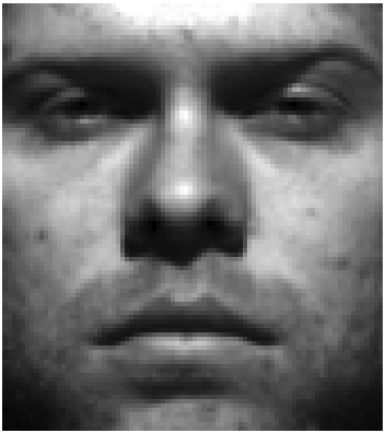
Refer to caption
Refer to caption
Refer to caption
Figure 10: Random pixel corruption of the face image [58] (from left to right): The noiseless image; The i.i.d random noise; The image with 90%percent9090\% of the pixels corrupted.
Refer to caption
Figure 11: Face recognition based on SRC under random pixel corruption using different sparsity regularization approaches.

In this case, the dictionary 𝑨𝑨{\bm{A}} is composed of two sub-dictionaries: 𝑨=[𝑨tr𝑰]𝑨subscript𝑨𝑡𝑟𝑰{\bm{A}}=[{\bm{A}}_{tr}\quad{\bm{I}}]. 𝑨trsubscript𝑨𝑡𝑟{\bm{A}}_{tr} is the collection of noiseless training samples that contributes to the “uncorrupted” test image, while 𝑰𝑰{\bm{I}} is the identity matrix that contributes to the random noise. 𝒙𝒙{\bm{x}} can then be separated into two parts accordingly: 𝒙T=[𝒙trT𝒙𝑰T]superscript𝒙𝑇superscriptsubscript𝒙𝑡𝑟𝑇superscriptsubscript𝒙𝑰𝑇{\bm{x}}^{T}=[{\bm{x}}_{tr}^{T}\quad{\bm{x}}_{{\bm{I}}}^{T}]. Based on the observation that the respective distributions of the entries in 𝒙trsubscript𝒙𝑡𝑟{\bm{x}}_{tr} and 𝒙𝑰Tsuperscriptsubscript𝒙𝑰𝑇{\bm{x}}_{{\bm{I}}}^{T} are quite different, we propose to regularize them using different regularization parameters as follows:

argmin𝒙𝒚𝑨𝒙22+λg(𝒙tr)+λμg(𝒙𝑰).subscript𝒙superscriptsubscriptnorm𝒚𝑨𝒙22𝜆𝑔subscript𝒙𝑡𝑟𝜆𝜇𝑔subscript𝒙𝑰\displaystyle\arg\min_{{\bm{x}}}\quad\quad\|{\bm{y}}-{\bm{A}}{\bm{x}}\|_{2}^{2}+\lambda\cdot g({\bm{x}}_{tr})+\lambda\mu\cdot g({\bm{x}}_{{\bm{I}}})\,. (77)

As done before, the parameters were tuned for each approach separately to obtain best performances. For the SEF minimization approach, p=1.2𝑝1.2p=1.2, λ=103𝜆superscript103\lambda=10^{-3}, μ=75𝜇75\mu=75; for the REF minimization approach, p=1.15𝑝1.15p=1.15, α=1.1𝛼1.1\alpha=1.1, λ=103𝜆superscript103\lambda=10^{-3}, μ=75𝜇75\mu=75; for the L1subscriptL1\textnormal{L}_{1} minimization approach, λ=103𝜆superscript103\lambda=10^{-3}, μ=2.5𝜇2.5\mu=2.5; for the Lp minimization approach, p=0.5𝑝0.5p=0.5, λ=104𝜆superscript104\lambda=10^{-4}, μ=5𝜇5\mu=5; for the L1/LsubscriptL1subscriptL\textnormal{L}_{1}/\textnormal{L}_{\infty} minimization approach, λ=106𝜆superscript106\lambda=10^{-6}, λ=2.5𝜆2.5\lambda=2.5; for the log\log-energy minimization approach, λ=106𝜆superscript106\lambda=10^{-6}, μ=5𝜇5\mu=5; for the IHT approach, λ=103𝜆superscript103\lambda=10^{-3}, μ=6𝜇6\mu=6. For the OMP and CoSaMP, the sparsity constraint on the training samples is set to Str20subscript𝑆𝑡𝑟20S_{tr}\leq 20, corresponding to the average number of samples per class in the experiments; the sparsity constraint on the noise is set to S𝑰7000subscript𝑆𝑰7000S_{{\bm{I}}}\leq 7000. The recognition rates of various approaches under increasing percentages of random pixel corruptions are shown in Fig. 11. We can see that the sparse representations obtained by minimizing the proposed SEF and REF lead to the highest recognition rates. The performance only starts to drop significantly when more than 90%percent9090\% of the pixels are corrupted.

V Conclusion and Future Work

In this paper we proposed the generalized Shannon entropy function hp(𝒙)subscript𝑝𝒙h_{p}({\bm{x}}) and Rényi entropy function hp,α(𝒙)subscript𝑝𝛼𝒙h_{p,\alpha}({\bm{x}}) as the sparsity regularizers for the sparse signal recovery task. Regardless of the values of p(0,]𝑝0p\in(0,\infty] and α(0,1)(1,]𝛼011\alpha\in(0,1)\cup(1,\infty], the local minimums of the generalized entropy functions occur on the boundaries of the orthants in Nsuperscript𝑁\mathbb{R}^{N}, and minimizing them produces sparse solutions. Both hp(𝒙)subscript𝑝𝒙h_{p}({\bm{x}}) and hp,α(𝒙)subscript𝑝𝛼𝒙h_{p,\alpha}({\bm{x}}) are nonconvex functions, the corresponding minimization problems (13),(14) can be solved via the adapted FISTA until convergence. Compared to other sparsity regularizers, minimizing the generalized entropy functions adaptively promotes multiple high-energy coefficients while suppressing the rest low-energy coefficients of the recovered solution.

Sparse signal recovery experiments on both the simulated and real data show the proposed entropy function regularizations perform better than OMP, CoSaMP and other popular sparsity regularizers, and achieve state-of-the-art performances. This motivates us to explore sufficient conditions for the uniqueness of the solution, seek matrices that satisfy such uniqueness conditions, and establish error bounds on the recovered signal 𝒙^^𝒙\hat{{\bm{x}}} in our future work. Additionally, we would like to apply the generalized entropy functions minimization approaches to other Compressive Sensing applications such as RPCA [71, 72, 73, 74], dictionary learning[75, 76, 77], etc.

Appendix A Monotonic Objective Function Minimization

Take the Shannon entropy function minimization (SEF) problem Php(𝒙)subscript𝑃subscript𝑝𝒙P_{h_{p}}({\bm{x}}) in (13) for example, we have the following:

F(𝒓)=f(𝒓)+λhp(𝒓)(a)f(𝒙(t))+𝒓𝒙(t),f(𝒙(t))+κ2𝒓𝒙(t)22+λhp(𝒓)=f(𝒙(t))12κf(𝒙(t))22+κ2𝒓(𝒙(t)1κf(𝒙(t)))22+λhp(𝒓)(b)f(𝒙(t))12κf(𝒙(t))22+κ2𝒙(t)(𝒙(t)1κf(𝒙(t)))22+λhp(𝒙(t))=f(𝒙(t))+λhp(𝒙(t))=F(𝒙(t)).𝐹𝒓𝑓𝒓𝜆subscript𝑝𝒓superscript(a)𝑓superscript𝒙𝑡𝒓superscript𝒙𝑡𝑓superscript𝒙𝑡𝜅2superscriptsubscriptdelimited-∥∥𝒓superscript𝒙𝑡22𝜆subscript𝑝𝒓𝑓superscript𝒙𝑡12𝜅superscriptsubscriptdelimited-∥∥𝑓superscript𝒙𝑡22𝜅2superscriptsubscriptdelimited-∥∥𝒓superscript𝒙𝑡1𝜅𝑓superscript𝒙𝑡22𝜆subscript𝑝𝒓superscript(b)𝑓superscript𝒙𝑡12𝜅superscriptsubscriptdelimited-∥∥𝑓superscript𝒙𝑡22𝜅2superscriptsubscriptdelimited-∥∥superscript𝒙𝑡superscript𝒙𝑡1𝜅𝑓superscript𝒙𝑡22𝜆subscript𝑝superscript𝒙𝑡𝑓superscript𝒙𝑡𝜆subscript𝑝superscript𝒙𝑡𝐹superscript𝒙𝑡\displaystyle\begin{split}F({\bm{r}})&=f({\bm{r}})+\lambda h_{p}({\bm{r}})\\ &\stackrel{{\scriptstyle\textnormal{(a)}}}{{\leq}}f({\bm{x}}^{(t)})+\left<{\bm{r}}-{\bm{x}}^{(t)},\nabla f({\bm{x}}^{(t)})\right>\\ &\quad+\frac{\kappa}{2}\left\|{\bm{r}}-{\bm{x}}^{(t)}\right\|_{2}^{2}+\lambda h_{p}({\bm{r}})\\ &=f({\bm{x}}^{(t)})-\frac{1}{2\kappa}\|\nabla f({\bm{x}}^{(t)})\|_{2}^{2}\\ &\quad+\frac{\kappa}{2}\left\|{\bm{r}}-\left({\bm{x}}^{(t)}-\frac{1}{\kappa}\nabla f({\bm{x}}^{(t)})\right)\right\|_{2}^{2}+\lambda h_{p}({\bm{r}})\\ &\stackrel{{\scriptstyle\textnormal{(b)}}}{{\leq}}f({\bm{x}}^{(t)})-\frac{1}{2\kappa}\|\nabla f({\bm{x}}^{(t)})\|_{2}^{2}\\ &\quad+\frac{\kappa}{2}\left\|{\bm{x}}^{(t)}-\left({\bm{x}}^{(t)}-\frac{1}{\kappa}\nabla f({\bm{x}}^{(t)})\right)\right\|_{2}^{2}+\lambda h_{p}({\bm{x}}^{(t)})\\ &=f({\bm{x}}^{(t)})+\lambda h_{p}({\bm{x}}^{(t)})\\ &=F({\bm{x}}^{(t)})\,.\end{split} (78)

The first inequality “(a)” is obtained using (49). The second inequality “(b)” holds because we enforce (51) when the nonconvex proximal operator (50) is inexactly solved. Combined with (69), the proposed Algorithm 1 is monotonic.

Additionally, we have:

  • hp(𝒙)subscript𝑝𝒙h_{p}({\bm{x}}) is continuous in Nsuperscript𝑁\mathbb{R}^{N}, hence it is also lower semi-continuous.

  • The data fidelity term f(𝒙)=𝒚𝑨𝒙220𝑓𝒙superscriptsubscriptnorm𝒚𝑨𝒙220f({\bm{x}})=\|{\bm{y}}-{\bm{A}}{\bm{x}}\|_{2}^{2}\geq 0 is bounded from below. f(𝒙)𝑓𝒙f({\bm{x}})\rightarrow\infty when 𝒙2subscriptnorm𝒙2\|{\bm{x}}\|_{2}\rightarrow\infty, hence f(𝒙)𝑓𝒙f({\bm{x}}) is coercive. hp(𝒙)0subscript𝑝𝒙0h_{p}({\bm{x}})\geq 0 is also bounded from below. Hence F(𝒙)=f(𝒙)+λhp(𝒙)𝐹𝒙𝑓𝒙𝜆subscript𝑝𝒙F({\bm{x}})=f({\bm{x}})+\lambda h_{p}({\bm{x}}) is coercive.

  • f(𝒙)𝑓𝒙f({\bm{x}}) has Lipschitz-continuous gradients [43].

Using Theorem 111 of [52], we can get that the proposed Algorithm 1 converges to a critical point.

Refer to caption
Refer to caption
Refer to caption
Refer to caption
Figure A12: Nonconvex soft shrinkage threshoding when the threshold τ(t)<0superscript𝜏𝑡0\tau^{(t)}<0.

Appendix B Energy-promoting Analysis of other regularization functions

Here we discuss the energy-promoting behaviors of the other sparsity regularizers666g10(𝒙)subscript𝑔10𝒙g_{10}({\bm{x}}) is not a sparsity regularizer. introduced in section I-A1 from an optimization perspective. Specifically, the regularizers are minimized via subderivative descent:

𝒙𝒙\displaystyle{\bm{x}} =𝒙ηhp(𝒙).absent𝒙𝜂subscript𝑝𝒙\displaystyle={\bm{x}}-\eta\cdot\partial h_{p}({\bm{x}})\,. (24 revisited)
  • The subderivatives of g1(𝒙)subscript𝑔1𝒙g_{1}({\bm{x}}), g2(𝒙)subscript𝑔2𝒙g_{2}({\bm{x}}), g5(𝒙)subscript𝑔5𝒙g_{5}({\bm{x}}) are as follows:

    xi𝒙1subscript𝑥𝑖subscriptnorm𝒙1\displaystyle\frac{\partial}{\partial x_{i}}\|{\bm{x}}\|_{1} =sign(xi)absentsignsubscript𝑥𝑖\displaystyle=\textnormal{sign}(x_{i}) (79)
    xi𝒙ppsubscript𝑥𝑖superscriptsubscriptnorm𝒙𝑝𝑝\displaystyle\frac{\partial}{\partial x_{i}}\|{\bm{x}}\|_{p}^{p} =sign(xi)p|xi|p1absentsignsubscript𝑥𝑖𝑝superscriptsubscript𝑥𝑖𝑝1\displaystyle=\textnormal{sign}(x_{i})\cdot p|x_{i}|^{p-1} (80)
    xii:|xi|0log|xi|2subscript𝑥𝑖subscript:𝑖subscript𝑥𝑖0superscriptsubscript𝑥𝑖2\displaystyle\frac{\partial}{\partial x_{i}}\sum_{i:|x_{i}|\neq 0}\log|x_{i}|^{2} =sign(xi)2|xi|.absentsignsubscript𝑥𝑖2subscript𝑥𝑖\displaystyle=\textnormal{sign}(x_{i})\cdot\frac{2}{|x_{i}|}\,. (81)

    The update (24) would decrease the magnitude of every coefficient.

  • The subderivatives of g3(𝒙)subscript𝑔3𝒙g_{3}({\bm{x}}), g4(𝒙)subscript𝑔4𝒙g_{4}({\bm{x}}) are:

    xi1𝒙subscript𝑥𝑖1subscriptnorm𝒙\displaystyle\frac{\partial}{\partial x_{i}}\frac{1}{\|{\bm{x}}\|_{\infty}} =sign(xi)δ(i)𝒙2absentsignsubscript𝑥𝑖subscript𝛿𝑖superscriptsubscriptnorm𝒙2\displaystyle=\textnormal{sign}(x_{i})\cdot\frac{-\delta_{\infty}(i)}{\|{\bm{x}}\|_{\infty}^{2}} (82)
    xi𝒙1N𝒙subscript𝑥𝑖subscriptnorm𝒙1𝑁subscriptnorm𝒙\displaystyle\frac{\partial}{\partial x_{i}}\frac{\|{\bm{x}}\|_{1}}{N\|{\bm{x}}\|_{\infty}} =sign(xi)N(1𝒙δ(i)𝒙1𝒙2),absentsignsubscript𝑥𝑖𝑁1subscriptnorm𝒙subscript𝛿𝑖subscriptnorm𝒙1superscriptsubscriptnorm𝒙2\displaystyle=\frac{\textnormal{sign}(x_{i})}{N}\cdot\left(\frac{1}{\|{\bm{x}}\|_{\infty}}-\delta_{\infty}(i)\frac{\|{\bm{x}}\|_{1}}{\|{\bm{x}}\|_{\infty}^{2}}\right)\,, (83)

    where δ(i)subscript𝛿𝑖\delta_{\infty}(i) is defined as follows:

    δ(i)={01if |xi|maxj|xj|if |xi|=maxj|xj|.subscript𝛿𝑖cases01if |xi|maxj|xj|if |xi|=maxj|xj|\displaystyle\delta_{\infty}(i)=\left\{\begin{array}[]{l}0\\ 1\end{array}\quad\begin{array}[]{l}\textnormal{if $|x_{i}|\neq\max_{j}|x_{j}|$}\\ \textnormal{if $|x_{i}|=\max_{j}|x_{j}|$}\,.\end{array}\right. (88)

    The update (24) would only increase the magnitude(s) of the highest-energy coefficient(s) for g3(𝒙)subscript𝑔3𝒙g_{3}({\bm{x}}) and g4(𝒙)subscript𝑔4𝒙g_{4}({\bm{x}}), while decreasing the magnitudes of the rest coefficients for g4(𝒙)subscript𝑔4𝒙g_{4}({\bm{x}}).

    We should note that the energy-promoting behaviors of g3(𝒙)subscript𝑔3𝒙g_{3}({\bm{x}}) and g4(𝒙)subscript𝑔4𝒙g_{4}({\bm{x}}) are different from those of the proposed entropy functions. For the entropy functions, the thresholds ν𝜈\nu in (32), (40) are adaptive in that they are updated every iteration along with the solution, as opposed to the rigid criterion induced by g3(𝒙)subscript𝑔3𝒙g_{3}({\bm{x}}) and g4(𝒙)subscript𝑔4𝒙g_{4}({\bm{x}}).

Appendix C Nonconvex Soft Shrinkage Thresholding

Take the optimization problem in (53) for example, let τi(t)=λκhp(|xi(t)|)superscriptsubscript𝜏𝑖𝑡𝜆𝜅subscript𝑝superscriptsubscript𝑥𝑖𝑡\tau_{i}^{(t)}=\frac{\lambda}{\kappa}\nabla h_{p}(|x_{i}^{(t)}|), si(t)=xi(t)1κf(xi(t))superscriptsubscript𝑠𝑖𝑡superscriptsubscript𝑥𝑖𝑡1𝜅𝑓superscriptsubscript𝑥𝑖𝑡s_{i}^{(t)}=x_{i}^{(t)}-\frac{1}{\kappa}\nabla f(x_{i}^{(t)}), we have the following problem for the i𝑖i-th entry xisubscript𝑥𝑖x_{i}:

minxi12xisi(t)22+τi(t)|xi|.subscriptsubscript𝑥𝑖12superscriptsubscriptnormsubscript𝑥𝑖superscriptsubscript𝑠𝑖𝑡22superscriptsubscript𝜏𝑖𝑡subscript𝑥𝑖\displaystyle\min_{x_{i}}\quad\frac{1}{2}\|x_{i}-s_{i}^{(t)}\|_{2}^{2}+\tau_{i}^{(t)}|x_{i}|\,. (89)
  • ❑ Positive threshold:

    When τi(t)0superscriptsubscript𝜏𝑖𝑡0\tau_{i}^{(t)}\geq 0, (89) is a convex problem. Its solution is given by applying the shrinkage operator given in (59) on si(t)superscriptsubscript𝑠𝑖𝑡s_{i}^{(t)} with the threshold τi(t)superscriptsubscript𝜏𝑖𝑡\tau_{i}^{(t)}.

  • ❑ Negative threshold:

    When τi(t)<0superscriptsubscript𝜏𝑖𝑡0\tau_{i}^{(t)}<0, (89) is a not necessarily a convex problem. Luckily this is a simple one dimensional problem, its global optimal solution can be still found as follows:

    1. 1.

      When si(t)<τi(t)superscriptsubscript𝑠𝑖𝑡superscriptsubscript𝜏𝑖𝑡s_{i}^{(t)}<\tau_{i}^{(t)}, as shown in Fig. A12:

      • For xi0subscript𝑥𝑖0x_{i}\geq 0, we have:

        minxi(xi+τi(t)si(t))2(τi(t)si(t))2+(si(t))2.\displaystyle\begin{split}\min_{x_{i}}\quad&\left(x_{i}+\tau_{i}^{(t)}-s_{i}^{(t)}\right)^{2}\\ &-\left(\tau_{i}^{(t)}-s_{i}^{(t)}\right)^{2}+\left(s_{i}^{(t)}\right)^{2}\,.\end{split} (90)

        Since τi(t)si(t)>0superscriptsubscript𝜏𝑖𝑡superscriptsubscript𝑠𝑖𝑡0\tau_{i}^{(t)}-s_{i}^{(t)}>0, the xisubscript𝑥𝑖x_{i} that minimizes (90) is 00.

      • For xi<0subscript𝑥𝑖0x_{i}<0, we have:

        minxi(xiτi(t)si(t))2(τi(t)+si(t))2+(si(t))2.\displaystyle\begin{split}\min_{x_{i}}\quad&\left(x_{i}-\tau_{i}^{(t)}-s_{i}^{(t)}\right)^{2}\\ &-\left(\tau_{i}^{(t)}+s_{i}^{(t)}\right)^{2}+\left(s_{i}^{(t)}\right)^{2}\,.\end{split} (91)

        Since τi(t)si(t)>0superscriptsubscript𝜏𝑖𝑡superscriptsubscript𝑠𝑖𝑡0-\tau_{i}^{(t)}-s_{i}^{(t)}>0, the xisubscript𝑥𝑖x_{i} that minimizes (91) is τi(t)+si(t)superscriptsubscript𝜏𝑖𝑡superscriptsubscript𝑠𝑖𝑡\tau_{i}^{(t)}+s_{i}^{(t)}.

      (89) is continuous at the point xi=0subscript𝑥𝑖0x_{i}=0. Hence the global minimum of (89) is obtained by xi=τi(t)+si(t)subscript𝑥𝑖superscriptsubscript𝜏𝑖𝑡superscriptsubscript𝑠𝑖𝑡x_{i}=\tau_{i}^{(t)}+s_{i}^{(t)}.

    2. 2.

      When τi(t)si(t)<0superscriptsubscript𝜏𝑖𝑡superscriptsubscript𝑠𝑖𝑡0\tau_{i}^{(t)}\leq s_{i}^{(t)}<0, as shown in Fig. A12:

      • For xi0subscript𝑥𝑖0x_{i}\geq 0, we have (90). Since τi(t)si(t)<0superscriptsubscript𝜏𝑖𝑡superscriptsubscript𝑠𝑖𝑡0\tau_{i}^{(t)}-s_{i}^{(t)}<0, the xisubscript𝑥𝑖x_{i} that minimizes (90) is τi(t)+si(t)superscriptsubscript𝜏𝑖𝑡superscriptsubscript𝑠𝑖𝑡-\tau_{i}^{(t)}+s_{i}^{(t)}.

      • For xi<0subscript𝑥𝑖0x_{i}<0, we have (91). Since τi(t)si(t)>0superscriptsubscript𝜏𝑖𝑡superscriptsubscript𝑠𝑖𝑡0-\tau_{i}^{(t)}-s_{i}^{(t)}>0, the xisubscript𝑥𝑖x_{i} that minimizes (91) is τi(t)+si(t)superscriptsubscript𝜏𝑖𝑡superscriptsubscript𝑠𝑖𝑡\tau_{i}^{(t)}+s_{i}^{(t)}.

      It’s easy to verify that the minimum of (91) is smaller than the minimum of (90). Hence the global minimum of (89) is obtained by τi(t)+si(t)superscriptsubscript𝜏𝑖𝑡superscriptsubscript𝑠𝑖𝑡\tau_{i}^{(t)}+s_{i}^{(t)}.

    3. 3.

      When 0si(t)<τi(t)0superscriptsubscript𝑠𝑖𝑡superscriptsubscript𝜏𝑖𝑡0\leq s_{i}^{(t)}<-\tau_{i}^{(t)}, as shown in Fig. A12:

      • For xi0subscript𝑥𝑖0x_{i}\geq 0, we have (90). Since τi(t)si(t)<0superscriptsubscript𝜏𝑖𝑡superscriptsubscript𝑠𝑖𝑡0\tau_{i}^{(t)}-s_{i}^{(t)}<0, the xisubscript𝑥𝑖x_{i} that minimizes (90) is τi(t)+si(t)superscriptsubscript𝜏𝑖𝑡superscriptsubscript𝑠𝑖𝑡-\tau_{i}^{(t)}+s_{i}^{(t)}.

      • For xi<0subscript𝑥𝑖0x_{i}<0, we have (91). Since τi(t)si(t)>0superscriptsubscript𝜏𝑖𝑡superscriptsubscript𝑠𝑖𝑡0-\tau_{i}^{(t)}-s_{i}^{(t)}>0, the xisubscript𝑥𝑖x_{i} that minimizes (91) is τi(t)+si(t)superscriptsubscript𝜏𝑖𝑡superscriptsubscript𝑠𝑖𝑡\tau_{i}^{(t)}+s_{i}^{(t)}.

      It’s easy to verify that the minimum of (91) is larger than the minimum of (90). Hence the global minimum of (89) is obtained by τi(t)+si(t)superscriptsubscript𝜏𝑖𝑡superscriptsubscript𝑠𝑖𝑡-\tau_{i}^{(t)}+s_{i}^{(t)}.

    4. 4.

      When si(t)τi(t)superscriptsubscript𝑠𝑖𝑡superscriptsubscript𝜏𝑖𝑡s_{i}^{(t)}\geq-\tau_{i}^{(t)}, as shown in Fig. A12:

      • For xi0subscript𝑥𝑖0x_{i}\geq 0, we have (90). Since τi(t)si(t)<0superscriptsubscript𝜏𝑖𝑡superscriptsubscript𝑠𝑖𝑡0\tau_{i}^{(t)}-s_{i}^{(t)}<0, the xisubscript𝑥𝑖x_{i} that minimizes (90) is τi(t)+si(t)superscriptsubscript𝜏𝑖𝑡superscriptsubscript𝑠𝑖𝑡-\tau_{i}^{(t)}+s_{i}^{(t)}.

      • For xi<0subscript𝑥𝑖0x_{i}<0, we have (91). Since τi(t)si(t)<0superscriptsubscript𝜏𝑖𝑡superscriptsubscript𝑠𝑖𝑡0-\tau_{i}^{(t)}-s_{i}^{(t)}<0, the xisubscript𝑥𝑖x_{i} that minimizes (91) is 00.

      (89) is continuous at the point xi=0subscript𝑥𝑖0x_{i}=0. Hence the global minimum of (89) is obtained by xi=τi(t)+si(t)subscript𝑥𝑖superscriptsubscript𝜏𝑖𝑡superscriptsubscript𝑠𝑖𝑡x_{i}=-\tau_{i}^{(t)}+s_{i}^{(t)}.

    Combining the above 444 different scenarios, we have the following results:

    1. 1.

      When si(t)0superscriptsubscript𝑠𝑖𝑡0s_{i}^{(t)}\geq 0, the solution to (89) is si(t)τi(t)superscriptsubscript𝑠𝑖𝑡superscriptsubscript𝜏𝑖𝑡s_{i}^{(t)}-\tau_{i}^{(t)}.

    2. 2.

      When si(t)<0superscriptsubscript𝑠𝑖𝑡0s_{i}^{(t)}<0, the solution to (89) is si(t)+τi(t)superscriptsubscript𝑠𝑖𝑡superscriptsubscript𝜏𝑖𝑡s_{i}^{(t)}+\tau_{i}^{(t)}.

    This is exactly the soft shrinkage operator given in (59) on si(t)superscriptsubscript𝑠𝑖𝑡s_{i}^{(t)} with the threshold τi(t)superscriptsubscript𝜏𝑖𝑡\tau_{i}^{(t)}.

Appendix D First-Order Approximations of Other Regularization Functions

  • g2(𝒙)=i=1N|xi|psubscript𝑔2𝒙superscriptsubscript𝑖1𝑁superscriptsubscript𝑥𝑖𝑝g_{2}({\bm{x}})=\sum_{i=1}^{N}|x_{i}|^{p}, where 𝒙N𝒙superscript𝑁{\bm{x}}\in\mathbb{R}^{N}. The function g2(𝒙)subscript𝑔2𝒙g_{2}({\bm{x}}) is continuous in its domain, hence it is also lower semi-continuous. The first-order approximation in (52) is updated accordingly:

    g2(𝒙)𝒙(t)pp+|𝒙||𝒙(t)|,g2(|𝒙(t)|),subscript𝑔2𝒙superscriptsubscriptdelimited-∥∥superscript𝒙𝑡𝑝𝑝𝒙superscript𝒙𝑡subscript𝑔2superscript𝒙𝑡\displaystyle\begin{split}g_{2}({\bm{x}})&\approx\|{\bm{x}}^{(t)}\|_{p}^{p}+\left<|{\bm{x}}|-|{\bm{x}}^{(t)}|,\nabla g_{2}(|{\bm{x}}^{(t)}|)\right>\,,\end{split} (92)

    where 0<p<10𝑝10<p<1. The gradient with respect to |xi|subscript𝑥𝑖|x_{i}| is:

    g2(𝒙)|xi|=p|xi|p1.subscript𝑔2𝒙subscript𝑥𝑖𝑝superscriptsubscript𝑥𝑖𝑝1\displaystyle\frac{\partial g_{2}({\bm{x}})}{\partial|x_{i}|}=p|x_{i}|^{p-1}\,. (93)
  • g4(𝒙)=𝒙1Nmaxj|xj|1subscript𝑔4𝒙subscriptnorm𝒙1𝑁subscript𝑗subscript𝑥𝑗1g_{4}({\bm{x}})=\frac{\|{\bm{x}}\|_{1}}{N\cdot\max_{j}|x_{j}|}-1, where 𝒙N𝒙superscript𝑁{\bm{x}}\in\mathbb{R}^{N} and 𝒙𝟎𝒙0{\bm{x}}\neq\bm{0}. The function g4(𝒙)subscript𝑔4𝒙g_{4}({\bm{x}}) is continuous in its domain. Hence it is also lower semi-continuous.

    Since g4(𝒙)subscript𝑔4𝒙g_{4}({\bm{x}}) is not differentiable with respect to the modulus |𝒙|𝒙|{\bm{x}}|, we use its subderivative to get the first order approximation:

    g4(𝒙)g4(|𝒙(t)|)+|𝒙||𝒙(t)|,g4(|𝒙(t)|).subscript𝑔4𝒙subscript𝑔4superscript𝒙𝑡𝒙superscript𝒙𝑡subscript𝑔4superscript𝒙𝑡\displaystyle\begin{split}g_{4}({\bm{x}})&\approx g_{4}(|{\bm{x}}^{(t)}|)+\left<|{\bm{x}}|-|{\bm{x}}^{(t)}|,\partial g_{4}(|{\bm{x}}^{(t)}|)\right>\,.\end{split} (94)

    The subderivative with respect to |xi|subscript𝑥𝑖|x_{i}| is:

    g4(𝒙)|xi|=1N(1𝒙δ(i)𝒙1𝒙2),subscript𝑔4𝒙subscript𝑥𝑖1𝑁1subscriptnorm𝒙subscript𝛿𝑖subscriptnorm𝒙1superscriptsubscriptnorm𝒙2\displaystyle\frac{\partial g_{4}({\bm{x}})}{\partial|x_{i}|}=\frac{1}{N}\left(\frac{1}{\|{\bm{x}}\|_{\infty}}-\delta_{\infty}(i)\frac{\|{\bm{x}}\|_{1}}{\|{\bm{x}}\|_{\infty}^{2}}\right)\,, (95)

    where δ(i)subscript𝛿𝑖\delta_{\infty}(i) is given in (88).

References

  • [1] D. L. Donoho, “Compressed sensing,” IEEE Trans. on Information Theory, vol. 52, no. 4, pp. 1289–1306, 2006.
  • [2] E. J. Candès, “Compressive sampling,” IEEE Proceedings of the International Congress of Mathematicians, 2006.
  • [3] E. J. Candès and M. B. Wakin, “An introduction to compressive sampling,” IEEE Signal Processing Magazine, vol. 25, no. 2, pp. 21–30, March 2008.
  • [4] E. Candès and T. Tao, “Decoding by linear programming,” IEEE Trans. on Information Theory, vol. 51(12), pp. 4203–4215, 2005.
  • [5] E. J. Candès, J. Romberg, and T. Tao, “Robust uncertainty principles: Exact signal reconstruction from highly incomplete frequency information,” IEEE Trans. on Information Theory, vol. 52, no. 2, pp. 489–509, 2006.
  • [6] E. J. Candès and T. Tao, “Near-optimal signal recovery from random projections: Universal encoding strategies?,” IEEE Trans. on Information Theory, vol. 52, no. 12, pp. 5406–5425, 2006.
  • [7] E. J. Candès, “The restricted isometry property and its implications for compressed sensing,” Comptes Rendus Mathematique, vol. 346, no. 9–10, pp. 589–592, 2008.
  • [8] B. K. Natarajan, “Sparse approximate aolutions to linear systems,” SIAM Journal on Computing, vol. 24, no. 2, pp. 227–234, 1995.
  • [9] G. Davis, Adaptive Nonlinear Approximations, PhD dissertation, New York University, 1994.
  • [10] T. Blumensath and M. E. Davies, “Iterative thresholding for sparse approximations,” Journal of Fourier Analysis and Applications, vol. 14, no. 5, pp. 629–654, Dec 2008.
  • [11] S. G. Mallat and Z. Zhang, “Matching pursuits with time-frequency dictionaries,” IEEE Transactions on Signal Processing, vol. 41, no. 12, pp. 3397–3415, 1993.
  • [12] J. A. Tropp and A. C. Gilbert, “Signal recovery from random measurements via orthogonal matching pursuit,” IEEE Transactions on Information Theory, vol. 53, no. 12, pp. 4655–4666, 2007.
  • [13] T. T. Cai and L. Wang, “Orthogonal matching pursuit for sparse signal recovery with noise,” IEEE Transactions on Information Theory, vol. 57, no. 7, pp. 4680–4688, July 2011.
  • [14] D. Needella and J. A. Tropp, “Cosamp: iterative signal recovery from incomplete and inaccurate samples,” Applied and Computational Harmonic Analysis, vol. 26, no. 3, pp. 301 – 321, 2009.
  • [15] W. Dai and O. Milenkovic, “Subspace pursuit for compressive sensing signal reconstruction,” IEEE Transactions on Information Theory, vol. 55, no. 5, pp. 2230–2249, 2009.
  • [16] T. Blumensath and M. E. Davies, “Iterative hard thresholding for compressed sensing,” Applied and Computational Harmonic Analysis, vol. 27, no. 3, pp. 265 – 274, 2009.
  • [17] T. Blumensath and M. E. Davies, “Normalized iterative hard thresholding: Guaranteed stability and performance,” IEEE Journal of Selected Topics in Signal Processing, vol. 4, no. 2, pp. 298–309, April 2010.
  • [18] S. Foucart, “Recovering jointly sparse vectors via hard thresholding pursuit,” in Proceedings of SampTA, Singapore, March 2011.
  • [19] K. Lee, Y. Bresler, and M. Junge, “Oblique pursuits for compressed sensing,” IEEE Transactions on Information Theory, vol. 59, no. 9, pp. 6111–6141, Sept 2013.
  • [20] N. Hurley and S. Rickard, “Comparing measures of sparsity,” IEEE Transactions on Information Theory, vol. 55, no. 10, pp. 4723–4741, Oct 2009.
  • [21] S. Huang, D. N. Tran, and T. D. Tran, “Sparse signal recovery based on nonconvex entropy minimization,” in 2016 IEEE International Conference on Image Processing (ICIP), Sept 2016, pp. 3867–3871.
  • [22] K. Kreutz-Delgado and B. D. Rao, “A general approach to sparse basis selection: majorization, concavity, and affine scaling,” Technical report, July 1997.
  • [23] R. R. Coifman and M. V. Wickerhauser, “Entropy-based algorithms for best basis selection,” IEEE Transactions on Information Theory, vol. 38, no. 2, pp. 713–718, March 1992.
  • [24] M. V. Wickerhauser, Adapted Wavelet Analysis from Theory to Software, A. K. Peters, Ltd., Natick, MA, USA, 1994.
  • [25] B. D. Rao and K. Kreutz-Delgado, “An affine scaling methodology for best basis selection,” IEEE Transactions on Signal Processing, vol. 47, no. 1, pp. 187–200, Jan 1999.
  • [26] D. L. Donoho, “On minimum entropy segmentation,” in Wavelets: theory, algorithms, and applications. 1994, pp. 233–269, Academic Press.
  • [27] E. J. Candès, J. K. Romberg, and T. Tao, “Stable signal recovery from incomplete and inaccurate measurements,” Communications on Pure and Applied Mathematics, vol. 59, no. 8, pp. 1207–1223, 2006.
  • [28] R. Chartrand, “Exact reconstructions of sparse signals via nonconvex minimization,” IEEE Signal Processing Letters, vol. 14, pp. 707–710, 2007.
  • [29] S. Foucart and M.-J. Lai, “Sparsest solutions of underdetermined linear systems via psubscript𝑝\ell_{p}-minimization for 0<p10𝑝10<p\leq 1,” Applied and Computational Harmonic Analysis, vol. 26, no. 3, pp. 395 – 407, 2009.
  • [30] D. Wipf and S. Nagarajan, “Iterative reweighted 1subscript1\ell_{1} and 2subscript2\ell_{2} methods for finding sparse solutions,” IEEE Journal of Selected Topics in Signal Processing, vol. 4, no. 2, pp. 317–329, April 2010.
  • [31] R. Chartrand and V. Staneva, “Restricted isometry properties and nonconvex compressive sensing,” Inverse Problems, vol. 24, no. 4, 2008.
  • [32] M. Pilanci, L. E. Ghaoui, and V. Chandrasekaran, “Recovery of sparse probability measures via convex programming,” in Advances in Neural Information Processing Systems 25, 2012, pp. 2420–2428.
  • [33] G. Pastor, I. Mora-Jimenez, R. Jantti, and A. J. Caamano, “Sparsity-based criteria for entropy measures,” in ISWCS 2013; The Tenth International Symposium on Wireless Communication Systems, Aug 2013, pp. 1–5.
  • [34] M. A. T. Figueiredo, “Adaptive sparseness for supervised learning,” IEEE Transactions on Pattern Analysis and Machine Intelligence, vol. 25, no. 9, pp. 1150–1159, Sept 2003.
  • [35] B. D. Rao, K. Engan, S. F. Cotter, J. Palmer, and K. Kreutz-Delgado, “Subset selection in noise based on diversity measure minimization,” IEEE Transactions on Signal Processing, vol. 51, no. 3, pp. 760–770, March 2003.
  • [36] E. J. Candès, M. B. Wakin, and S. P. Boyd, “Enhancing sparsity by reweighted 1subscript1\ell_{1}- minimization,” Journal of Fourier Analysis and Applications, vol. 14, no. 5, pp. 877–905, 2008.
  • [37] K. Kose, O. Gunay, and A. E. Ceti, “Compressive sensing using the modified entropy functional,” Digital Signal Processing, vol. 24, pp. 63–70, 2014.
  • [38] M. A. T. Figueiredo, R. D. Nowak, and S. J. Wright, “Gradient projection for sparse reconstruction: Application to compressed sensing and other inverse problems,” IEEE Journal of Selected Topics in Signal Processing, vol. 1, no. 4, pp. 586–597, Dec 2007.
  • [39] A. Chambolle, R. A. D. Vore, N.-Y. Lee, and B. J. Lucier, “Nonlinear wavelet image processing: variational problems, compression, and noise removal through wavelet shrinkage,” IEEE Transactions on Image Processing, vol. 7, no. 3, pp. 319–335, March 1998.
  • [40] M. A. T. Figueiredo and R. D. Nowak, “An em algorithm for wavelet-based image restoration,” IEEE Transactions on Image Processing, vol. 12, no. 8, pp. 906–916, Aug 2003.
  • [41] I. Daubechies, M. Defrise, and C. De Mol, “An iterative thresholding algorithm for linear inverse problems with a sparsity constraint,” Communications on Pure and Applied Mathematics, vol. 57, no. 11, pp. 1413–1457, 2004.
  • [42] J. M. Bioucas-Dias and M. A. T. Figueiredo, “A new twist: Two-step iterative shrinkage/thresholding algorithms for image restoration,” IEEE Transactions on Image Processing, vol. 16, no. 12, pp. 2992–3004, Dec 2007.
  • [43] A. Beck and M. Teboulle, “A fast iterative shrinkage-thresholding algorithm for linear inverse problems,” SIAM Journal on Imaging Sciences, vol. 2, no. 1, pp. 183–202, 2009.
  • [44] A. Beck and M. Teboulle, “Fast gradient-based algorithms for constrained total variation image denoising and deblurring problems,” IEEE Transactions on Image Processing, vol. 18, pp. 2419–2434, 2009.
  • [45] Y. Nesterov, “A method of solving a convex programming problem with convergence rate o(1/k2)𝑜1superscript𝑘2o(1/k^{2}),” Soviet Mathematics Doklady, vol. 27, no. 2, pp. 372–376, 1983.
  • [46] S. Becker, J. Bobin, and E. J. Candès, “Nesta: A fast and accurate first-order method for sparse recovery,” SIAM Journal on Imaging Sciences, vol. 4, no. 1, pp. 1–39, 2011.
  • [47] J. Yang and Y. Zhang, “Alternating direction algorithms for _1_1\ell\_1-problems in compressive sensing,” SIAM Journal on Scientific Computing, vol. 33, no. 1, pp. 250–278, 2011.
  • [48] A. Y. Yang, A. Ganesh, Z. Zhou, S. S. Sastry, and Y. Ma, “A review of fast l1-minimization algorithms for robust face recognition,” CoRR, vol. abs/1007.3753, 2010.
  • [49] A. Y. Yang, Z. Zhou, A. G. Balasubramanian, S. S. Sastry, and Y. Ma, “Fast 1subscript1\ell_{1}-minimization algorithms for robust face recognition.,” IEEE Transactions on Image Processing, vol. 22, no. 8, pp. 3234–3246, May 2013.
  • [50] B. Martinet, “Brève communication. régularisation d’inéquations variationnelles par approximations successives,” ESAIM: Mathematical Modelling and Numerical Analysis - Modélisation Mathématique et Analyse Numérique, vol. 4, no. R3, pp. 154–158, 1970.
  • [51] N. Parikh and S. Boyd, “Proximal algorithms,” Foundations and Trends in Optimization, vol. 1, no. 3, pp. 123–231, 2013.
  • [52] H. Li and Z. Lin, “Accelerated proximal gradient methods for nonconvex programming,” in Advances in Neural Information Processing Systems 28, 2015, pp. 379–387.
  • [53] T. M. Cover and J. A. Thomas, Elements of information theory, Wiley-Interscience, 2006.
  • [54] A. Rényi, “On measures of information and entropy,” in Proceedings of the 4th Berkeley symposium on mathematics, statistics and probability, 1960, vol. 1, pp. 547–561.
  • [55] M. Ben-Bassat and J. Raviv, “Rényi’s entropy and the probability of error,” IEEE Transactions on Information Theory, vol. 24, no. 3, pp. 324–331, May 1978.
  • [56] G. M. Bosyk, S. Zozor, F. Holik, M. Portesi, and P. W. Lamberti, “A family of generalized quantum entropies: definition and properties,” Quantum Information Processing, vol. 15, no. 8, pp. 3393–3420, 2016.
  • [57] P. A. Bromiley, N. A. Thacker, and E. Bouhova-Thacker, “Shannon entropy, rényi entropy, and information,” Tech. Rep., Tina Memo No. 2004-004, 2004.
  • [58] J. Wright, A. Y. Yang, A. Ganesh, S. S. Sastry, and Y. Ma, “Robust face recognition via sparse representation,” IEEE Transactions on Pattern Analysis and Machine Intelligence, vol. 31, no. 2, pp. 210–227, Feb 2009.
  • [59] J. Wright, Y. Ma, J. Mairal, G. Sapiro, T. S. Huang, and S. Yan, “Sparse sepresentation for computer vision and pattern recognition,” Proceedings of the IEEE, vol. 98, no. 6, pp. 1031–1044, June 2010.
  • [60] K. Eriksson, D. Estep, and C. Johnson, “Applied mathematics body and soul: Vol i: derivatives and geometry in ir3,” Springer-Verlag Publishing, pp. 149–164, 2004.
  • [61] S. J. Reddi, S. Sra, B. Poczos, and A. J. Smola, “Proximal stochastic methods for nonsmooth nonconvex finite-sum optimization,” in Advances in Neural Information Processing Systems 29, D. D. Lee, M. Sugiyama, U. V. Luxburg, I. Guyon, and R. Garnett, Eds., 2016, pp. 1145–1153.
  • [62] Q. Yao, J. T. Kwok, F. Gao, W. Chen, and T.-Y. Liu, “Efficient inexact proximal gradient algorithm for nonconvex problems,” in Proceedings of the Twenty-Sixth International Joint Conference on Artificial Intelligence, IJCAI-17, 2017, pp. 3308–3314.
  • [63] B. D. Rao, K. Engan, S. F. Cotter, J. Palmer, and K. Kreutz-Delgado, “Subset selection in noise based on diversity measure minimization,” IEEE Transactions on Signal Processing, vol. 51, no. 3, pp. 760–770, March 2003.
  • [64] I. F. Gorodnitsky and B. D. Rao, “Sparse signal reconstruction from limited data using focuss: a re-weighted minimum norm algorithm,” IEEE Transactions on Signal Processing, vol. 45, no. 3, pp. 600–616, Mar 1997.
  • [65] R. E. Carrillo, J. D. McEwen, D. V. D. Ville, J. P. Thiran, and Y. Wiaux, “Sparsity averaging for compressive imaging,” IEEE Signal Processing Letters, vol. 20, no. 6, pp. 591–594, June 2013.
  • [66] I. Daubechies, Ten lectures on wavelets, Society for Industrial and Applied Mathematics, Philadelphia, PA, USA, 1992.
  • [67] T. T. Do, L. Gan, N. H. Nguyen, and T. D. Tran, “Fast and efficient compressive sensing using structurally random matrices,” IEEE Transactions on Signal Processing, vol. 60, no. 1, pp. 139–154, Jan 2012.
  • [68] S. Nam, M. Davies, M. Elad, and R. Gribonval, “The cosparse analysis model and algorithms,” Applied and Computational Harmonic Analysis, vol. 34, no. 1, pp. 30 – 56, 2013.
  • [69] S. Setzer, Split Bregman algorithm, Douglas-Rachford splitting and frame shrinkage, pp. 464–476, Springer Berlin Heidelberg, Berlin, Heidelberg, June 2009.
  • [70] A. S. Georghiades, P. N. Belhumeur, and D. J. Kriegman, “From few to many: illumination cone models for face recognition under variable lighting and pose,” IEEE Transactions on Pattern Analysis and Machine Intelligence, vol. 23, no. 6, pp. 643–660, June 2001.
  • [71] J. Wright, A. Ganesh, S. Rao, Y. Peng, and Y. Ma, “Robust principal component analysis: exact recovery of corrupted low-rank matrices via convex optimization,” in Advances in Neural Information Processing Systems, pp. 2080–2088. Curran Associates, Inc., 2009.
  • [72] Z. Lin, M. Chen, and Y. Ma, “The augmented lagrange multiplier method for exact recovery of corrupted low-rank matrices,” UIUC Technical Report, , no. UILU-ENG-09-2215, 2009.
  • [73] Z. Lin, A. Ganesh, J. Wright, L. Wu, M. Chen, and Y. Ma, “Fast convex optimization algorithms for exact recovery of a corrupted low-rank matrix,” UIUC Technical Report, , no. UILU-ENG-09-2214, 2009.
  • [74] E. J. Candès, X. Li, Y. Ma, and J. Wright, “Robust principal component analysis?,” Journal of the ACM, vol. 58, no. 3, pp. 11:1–11:37, May 2011.
  • [75] M. Aharon, M. Elad, and A. Bruckstein, “k -svd: An algorithm for designing overcomplete dictionaries for sparse representation,” IEEE Transactions on Signal Processing, vol. 54, no. 11, pp. 4311–4322, Nov 2006.
  • [76] M. Elad and M. Aharon, “Image denoising via sparse and redundant representations over learned dictionaries,” IEEE Transactions on Image Processing, vol. 15, no. 12, pp. 3736–3745, Dec 2006.
  • [77] J. Mairal, F. Bach, J. Ponce, and G. Sapiro, “Online dictionary learning for sparse coding,” in Proceedings of the 26th Annual International Conference on Machine Learning, 2009, pp. 689–696.