Technical Report on Two-Step Knowledge-Aided Iterative ESPRIT Algorithm

Abstract

In this work, we propose a subspace-based algorithm for direction-of-arrival (DOA) estimation, referred to as two-step knowledge-aided iterative estimation of signal parameters via rotational invariance techniques (ESPRIT) method (Two-Step KAI-ESPRIT), which achieves more accurate estimates than those of prior art. The proposed Two-Step KAI-ESPRIT improves the estimation of the covariance matrix of the input data by incorporating prior knowledge of signals and by exploiting knowledge of the structure of the covariance matrix and its perturbation terms. Simulation results illustrate the improvement achieved by the proposed method.

I Introduction

In array signal processing, direction-of-arrival (DOA) estimation is a key task in a broad range of important applications including radar and sonar systems, wireless communications and seismology [1, 2, 3, 4, 5, 6, 7, 8, 9, 10, 11, 12, 13, 14, 28, 17, 16, 19, 18, 20, 22, 21, 24, 25, 26, 31, 32, 29, 30, 23, 56, 35, 33, 34, 39, 37, 38, 39, 40, 41, 42, 43, 44, 46, 48, 49, 53, 54, 55, 56, 58, 59, 60]. Classical high-resolution methods for DOA estimation such as the multiple signal classification (MUSIC) method [61], the root-MUSIC algorithm [62], the estimation of signal parameters via rotational invariance techniques (ESPRIT) [63] and other recent subspace techniques [64, 65, 66] are based on estimating the signal and noise subspaces from the sample covariance matrix. The accuracy of the estimates of the covariance matrix is of fundamental importance in parameter estimation. In practical scenarios, only a limited number of samples is available and when the number of samples is comparable to the number of sensor array elements, the estimated and the true subspaces can significantly diverge. This problem has been dealt with using random matrix theory in [67, 68, 69], and the development of G-MUSIC, which considers the asymptotic situation when both the sample size and the number of array elements tend to infinity at the same rate. It is then deduced that the introduced method more accurately describes the case in which these two quantities are finite and similar in magnitude [69].

In this work, we take into account a different approach to improve the quality of the sample covariance matrix estimate in the finite sample size region. Inspired by the structural approach of [72, 73] and the use of prior knowledge about signals [70, 71], we develop an ESPRIT-based technique that exploits both prior knowledge about signals and the structure of the covariance matrix to improve the estimation accuracy. Our approach determines the value of a scaling factor that reduces the undesirable terms causing perturbations in the estimation of the signal and noise subspaces in an iterative manner, resulting in better estimates. This is done by choosing the set of DOA estimates that have higher likelihood of being the set of true DOAs. Furthermore, whereas in [72, 73], the undesirable terms are calculated based on steering vectors of estimates, in the proposed method this computation makes use not only of those estimates but also of the available prior knowledge of DOAs. Considering a practical scenario, this task can be achieved using signals coming from base stations or from static users in the system.

The remainder of this paper is organized as follows. Section II describes the system model and its parameters. Section III presents the proposed Two-Step KAI-ESPRIT algorithm. In section IV, we deal with the computational complexity analysis by means of counting the multiplications and additions involved in the processing. Section V illustrates and discusses the simulation results and finally, the concluding remarks are drawn in Section VI.

II System Model and Background

Let us assume that P uncorrelated narrowband signals from far-field sources impinge on a uniform linear array (ULA) of $M\ (M>\textit{P})$ sensor elements from directions ${\bm{\theta}}=[\theta_{1},\theta_{2},\ldots,\theta_{P}]^{T}$. We also consider that the sensors are spaced from each other by a distance $d\leq\frac{\lambda_{c}}{2}$, where $\lambda_{c}$ is the signal wavelength, and that without loss of generality, we have ${\frac{-\pi}{2}\leq\theta_{1}\leq\theta_{2}\ldots\leq\theta_{P}\leq\frac{-\pi}{2}}$.

The $i$th data snapshot of the $M$-dimensional array output vector can be modeled as

$$\bm{x}(i)=\bm{A}\,s(i)+\bm{n}(i),\qquad i=1,2,\ldots,N,$$ (1)

where $\bm{s}(i)=[s_{1}(i),\ldots,s_{P}(i)]^{T}\in\mathbb{C}^{\mathit{P\times 1}}$ represents the zero-mean source data vector, $\bm{n}(i)\in\mathbb{C}^{\mathit{M\times 1}}$ is the vector of white circular complex Gaussian noise with zero mean and variance $\sigma_{n}^{2}$, and $N$ denotes the number of available snapshots. The Vandermonde matrix $\bm{A}(\bm{\Theta})=[\bm{a}(\theta_{1}),\ldots,\bm{a}(\theta_{P})]\in\mathbb{C}^{\mathit{M\times P}}$, known as the array manifold, contains the array steering vectors $\bm{a}(\theta_{j})$ corresponding to the $n$th source, which can be expressed as

$$\bm{a}(\theta_{n})=[1,e^{j2\pi\frac{d}{\lambda_{c}}\sin\theta_{n}},\ldots,e^{j2\pi(M-1)\frac{d}{\lambda_{c}}\sin\theta_{n}}]^{T},$$ (2)

where $n=1,\ldots,P$. Using the fact that $\bm{s}(i)$ and $\bm{n}(i)$ are modeled as uncorrelated linearly independent variables, the $M\times M$ signal covariance matrix is calculated by

$$\bm{R}=\mathbb{E}\left[\bm{x}(i)\bm{x}^{H}(i)\right]=\bm{A}\,\bm{R}_{ss}\bm{A}^{H}+\sigma_{n}^{2}\bm{I}_{M},$$ (3)

where the superscript H and $\mathbb{E}[\cdot]$ in $\bm{R}_{ss}=\mathbb{E}[\bm{s}(i)\bm{s}^{H}(i)]$ and in $\mathbb{E}[\bm{n}(i)\bm{n}^{H}(i)]=\sigma_{n}^{2}\bm{I}_{M}$ denote the Hermitian transposition and the expectation operator and $\bm{I}_{M}$ stands for the $M\times M$ identity matrix. Since the true signal covariance matrix is unknown, it must be estimated and a widely-adopted approach is the sample average formula given by

$$\bm{\hat{R}}=\frac{1}{N}\sum\limits^{N}_{i=1}\bm{x}(i)\bm{x}^{H}(i),$$ (4)

whose estimation accuracy is dependent on the number of snapshots.

III Proposed Two-Step KAI-ESPRIT Algorithm

In this section, we present the proposed two-step KAI-ESPRIT algorithm and detail its main features.

We can start by expanding (4) using (1) as follows:

$$\bm{\hat{R}}=\frac{1}{N}\sum\limits^{N}_{i=1}(\bm{A}\,s(i)+\bm{n}(i))\>(\bm{A}\,s(i)+\bm{n}(i))^{H}$$

$$=\bm{A}\left\{\frac{1}{N}\sum\limits^{N}_{i=1}\bm{s}(i)\bm{s}^{H}(i)\right\}\bm{A}^{H}+\>\frac{1}{N}\sum\limits^{N}_{i=1}\bm{n}(i)\bm{n}^{H}(i)\;+$$

$$\bm{A}\left\{\frac{1}{N}\sum\limits^{N}_{i=1}\bm{s}(i)\bm{n}^{H}(i)\right\}\>+\>\left\{\frac{1}{N}\sum\limits^{N}_{i=1}\bm{n}(i)\bm{s}^{H}(i)\right\}\bm{A}^{H}$$ (5)

The first two terms of $\bm{\hat{R}}$ in (5) can be considered as estimates of the two summands of $\bm{R}$ given in (3), which represent the signal and the noise components, respectively. The last two terms in (5) are undesirable by-products, which can be seen as estimates for the correlation between the signal and the noise vectors. The system model under study is based on noise vectors which are zero-mean and also independent of the signal vectors. Thus, the signal and noise components are uncorrelated to each other. As a consequence, for a large enough number of samples N, the last two terms of (5) tend to zero. Nevertheless, in practice the number of available samples can be limited. In such situations, the last two terms in (5) may have significant values, which causes the deviation of the estimates of the signal and the noise subspaces from the true signal and noise ones. The key point of the proposed Two-Step KAI-ESPRIT algorithm is to modify the sample data covariance matrix in the second step based on the estimates obtained at the first step and the available known DOAs. The modified covariance matrix is computed by deriving a scaled version of the undesirable terms from $\bm{\hat{R}}$.

The steps of the proposed algorithm are listed in Table I. The algorithm starts by computing the sample data covariance matrix (4). Next, the DOAs are estimated using the ESPRIT algorithm. The superscript $(\cdot)^{(1)}$ refers to the estimation task performed in the first step. In the second step, the Vandermonde matrix is formed using the DOA estimates. Then, the amplitudes of the sources are estimated such that the square norm of the differences between the observation vector and the vector containing estimates and the available known DOAs is minimized. This problem can be formulated as

$$\hat{\bm{s}}(i)=\arg\min_{\begin{subarray}{c}\bm{s}\end{subarray}}\parallel\bm{x}(i)-\hat{\bm{A}}\mathbf{s}\parallel^{2}_{2}.$$ (6)

The minimization of (6) is achieved using the least squares technique and the solution is described by

$$\hat{\bm{s}}(i)=(\mathbf{\hat{A}}^{H}\>\mathbf{\hat{A}})^{-1}\>\mathbf{\hat{A}}\>\bm{x}(i)$$ (7)

The noise component is then estimated as the difference between the estimated signal and the observations made by the array, as given by

$$\hat{\bm{n}}(i)=\bm{x}(i)\>-\>\hat{\bm{A}}\>\hat{\bm{s}}(i).$$ (8)

After estimating the signal and noise vectors, the third term in (5) can be computed as

$$\bm{V} \triangleq\hat{\bm{A}}\left\{\frac{1}{N}\sum\limits^{N}_{i=1}\bm{\hat{}}{\mathbf{s}}(i)\bm{\hat{}}{\mathbf{n}}^{H}(i)\right\}$$

$$=\hat{\bm{A}}\left\{\frac{1}{N}\sum\limits^{N}_{i=1}(\mathbf{\hat{A}}^{H}\>\mathbf{\hat{A}})^{-1}\mathbf{\hat{A}}^{H}\bm{x}(i)\right.$$

$$\left.\times(\bm{x}^{H}(i)-\bm{x}^{H}(i)\hat{\mathbf{A}}(\hat{\mathbf{A}}^{H}\hat{\mathbf{A}})^{-1}\>\hat{\mathbf{A}}^{H})\right\}$$

$$=\mathbf{\hat{Q}}_{A}\left\{\frac{1}{N}\sum\limits^{N}_{i=1}\bm{x}(i)\bm{x}^{H}(i)\>\left(\mathbf{I}_{M}\>-\>\hat{\mathbf{Q}}_{A}\right)\right\}$$

$$=\mathbf{\hat{Q}}_{A}\>\mathbf{\hat{R}}\>\mathbf{\hat{Q}}_{A}^{\perp},$$ (9)

where

$$\mathbf{\hat{Q}}_{A}\triangleq\mathbf{\hat{A}}\>(\mathbf{\hat{A}}^{H}\>\mathbf{\hat{A}})^{-1}\>\mathbf{\hat{A}}^{H}$$ (10)

is an estimate of the projection matrix of the signal subspace, and

$$\mathbf{\hat{Q}}_{A}^{\perp}\triangleq\mathbf{I}_{M}\>-\>\mathbf{\hat{Q}}_{A}$$ (11)

is an estimate of the projection matrix of the noise subspace.

Lastly, the modified data covariance matrix is calculated by computing a scaled version of the estimated terms from the initial sample data covariance matrix as given

$$\mathbf{\hat{R}}^{(n+1)}=\mathbf{\hat{R}}\>-\>\mathrm{\mu}\>(\mathbf{V}^{(n)}\>+\>\mathbf{V}^{(n)H}),\hskip 8.53581pt\textit{n}\hskip 2.84526pt=\hskip 2.84526pt\text{1}$$ (12)

The scaling or reliability factor $\mu$ increases from 0 to 1 incrementally, resulting in modified data covariance matrices. Each of them gives origin to new estimated DOAs denoted by the superscript $(\cdot)^{(2)}$ by using the ESPRIT algorithm, as briefly described ahead. Assuming the rank P is known, the eigenvalue decomposition (EVD) of the modified data covariance matrix (12) yields

$$\begin{array}[]{ccc}\mathbf{\hat{R}}^{(n+1)}\end{array}=\left[\begin{array}[]{ccc}\mathbf{\hat{U}}_{s}&\mathbf{\hat{U}}_{n}\\ \end{array}\right]\left[\begin{array}[]{ccc}\mathbf{\hat{\Lambda}}_{s}&0\\ 0&\mathbf{\hat{\Lambda}}_{n}\end{array}\right]\left[\begin{array}[]{ccc}\mathbf{\hat{U}}_{s}^{H}\\ \mathbf{\hat{U}}_{n}^{H}\end{array}\right]$$ (13)

where the matrix $\mathbf{\hat{U}}_{s}$ $\in$ $\mathbb{C}^{\mathit{M\times P}}$ represents the signal subspace and the matrix $\mathbf{\hat{U}}_{n}$ $\in$ $\mathbb{C}^{\mathit{M\times(M-P)}}$ represents the the noise subspace respectively. The diagonal matrices $\mathbf{\hat{\Lambda}_{s}}$ and $\mathbf{\hat{\Lambda}_{n}}$ contain the P largest and the M-P smallest eigenvalues, respectively. We can form a twofold subarray configuration, as each row of the (Vandermonde) array steering matrix $\bm{A}(\bm{\Theta})$ corresponds to one particular sensor element of the antenna array. The subarrays are specified by two $\mathit{(s\times M)}$-dimensional selection matrices $\mathbf{J_{1}}$ and $\mathbf{J_{2}}$ which choose $\mathit{s}$ elements of the $\mathit{M}$ existing sensors respectively, where $\mathit{s}$ is in the range $\mathit{P\leq s<M}$. For maximum overlap, the matrix $\mathbf{J_{1}}$ selects the first $\mathit{s=M-1}$ elements and the matrix $\mathbf{J_{2}}$ selects the last $\mathit{s=M-1}$ rows of $\bm{A}(\bm{\Theta})$.

Since the matrices $\mathbf{J_{1}}$ and $\mathbf{J_{2}}$ have now been computed, we can estimate the operator $\mathbf{\Psi}$ by solving the approximation of the shift invariance equation (14) given by

$$\mathbf{J}_{1}\>\mathbf{\hat{U}}_{s}\>\mathbf{\Psi}\>\approx\>\mathbf{J}_{2}\>\mathbf{\hat{U}}_{s}$$ (14)

Using the least square (LS) method, which yields

$$\hat{\mathbf{\Psi}}=\arg\min_{\begin{subarray}{c}\mathbf{\Psi}\end{subarray}}\parallel\mathbf{J}_{2}\>\mathbf{\hat{U}}_{s}\>-\>\mathbf{J}_{1}\>\mathbf{\hat{U}}_{s}\>\mathbf{\Psi}\parallel_{F}\>=\>\left(\mathbf{J}_{1}\>\hat{\mathbf{U}}_{s}\right)^{\dagger}\>\mathbf{J}_{2}\>\hat{\mathbf{U}}_{s},$$ (15)

where $\parallel\cdot\parallel_{F}$ denotes the Frobenius norm and $\left(\cdot\right)^{\dagger}$ stands for the pseudo-inverse.

Lastly, the eigenvalues $\lambda_{n}$ of $\hat{\mathbf{\Psi}}$ contain the estimates of the spatial frequencies $\gamma_{n}$ computed as

$$\gamma_{n}\>=\>\arg\left(\lambda_{n}\right)$$ (16)

so that the DOAs can be calculated as

$$\hat{\theta}_{n}\>=\>\arcsin\left(\frac{\gamma_{n}\>\lambda_{c}}{2\pi\>\mathit{d}}\right)$$ (17)

where for (16) and (17) $\mathrm{n=1,\cdots,P}$.

Then, a new Vandermonde matrix is formed by the steering vectors of those newly estimated DOAs and the available known DOAs. By using the new matrix, it is possible to compute the new estimates of the projection matrices of the signal $\mathbf{\hat{Q}}_{A}^{(n)}$ and the noise $\mathbf{\hat{Q}}_{A}^{(n)\perp}$ subspaces, both for n=2.

Next, employing the new estimates of the projection matrices, the initial sample data matrix, $\bm{\hat{R}}$, and the number of sensors and sources, the stochastic maximum likelihood objective function [74] is computed for each value of $\mu$, as follows:

$$\mathit{U(\mu)}\,=\,\mathrm{ln\>det}\>\left(\mathbf{\hat{Q}}_{A}^{(2)}\>\mathbf{\hat{R}}\>\mathbf{\hat{Q}}_{A}^{(2)}\>+\>\dfrac{{\rm Trace}\{\mathbf{\hat{Q}}_{A}^{\perp\>(2)}\>\mathbf{\hat{R}}\}}{\mathrm{M-P}}\>\mathbf{\hat{Q}}_{A}^{\perp\>(2)}\right)$$ (18)

The previous computation selects the set of unavailable DOA estimates that have a higher likelihood. Then, the set of estimated DOAs corresponding to the optimum value of $\mu$ that minimizes (18) is determined. Finally, the output of the proposed Two-Step KAI-ESPRIT algorithm is formed by the set of available known DOAs and the estimates of the unavailable DOAs, as described in Table I.

TABLE I: Proposed Two-Step KAI-ESPRIT Algorithm

Inputs:

$\mathit{M}$,  $\mathit{d}$,  $\lambda$,  $\mathit{N}$,  $\mathit{P}$

Received vectors $\bm{x}(1)$,  $\bm{x}(2)$,$\cdots$, $\bm{x}(N)$

Prior knowledge $\rightarrow$ known DOAs:  $\mathit{\theta}_{1}$,  $\mathit{\theta}_{2}$, $\cdots$,  $\mathit{\theta}_{q}$   $\mathit{1\leq q<P}$

Outputs:

Estimates $\mathit{\hat{\theta}_{q+1}^{(2)}}$,  $\mathit{\hat{\theta}_{q+2}^{(2)}}$,$\cdots$,  $\mathit{\hat{\theta}_{P}^{(2)}}$

First step:

$\mathbf{\hat{R}}=\frac{1}{N}\sum\limits^{N}_{i=1}\bm{x}(i)\bm{x}^{H}(i)$

$\{\mathit{\hat{\theta}_{1}}^{(1)},\>\mathit{\hat{\theta}_{2}}^{(1)},\cdots,\mathit{\hat{\theta}_{P}}^{(1)}\}\;\;\underleftarrow{ESPRIT}$ $\>(\mathbf{\hat{R}},P,d,\lambda)$

Second step:

$\mathbf{\hat{A}}^{(1)}=\left[\mathbf{a}(\mathit{\hat{\theta}}_{1}^{(1)}),\mathbf{a}({\mathit{\hat{\theta}}_{2}^{(1)}}),\>\cdots,\mathbf{a}(\mathit{\hat{\theta}_{P}^{(1)}})\right]$

compute for n = 1

$\mathbf{\hat{Q}}_{A}^{(n)}=\mathbf{\hat{A}}^{(n)}\>(\mathbf{\hat{A}}^{(n)H}\>\mathbf{\hat{A}}^{(n)})^{-1}\>\mathbf{\hat{A}}^{(n)H}$       (1)

$\mathbf{\hat{Q}}_{A}^{(n)\perp}=\mathbf{I}_{M}\>-\>\mathbf{\hat{Q}}_{A}^{(n)}$                           (2)

$\mathbf{V}^{(n)}=\mathbf{\hat{Q}}_{A}^{(n)}\>\mathbf{\hat{R}}\>\mathbf{\hat{Q}}_{A}^{(n)\perp}$

for $\mathbf{\mu=}\hskip 2.84526pt\text{0}:\text{increment\hskip 2.84526pt:\hskip 2.84526pt1}$

compute   $\mathbf{\hat{R}}^{(n+1)}=\mathbf{\hat{R}}\>-\>\mathrm{\mu}\>(\mathbf{V}^{(n)}\>+\>\mathbf{V}^{(n)H})$,   n = 1

$\{\mathit{\hat{\theta}_{q+1}}^{(2)},\>\mathit{\hat{\theta}_{q+2}}^{(2)},\cdots,\mathit{\hat{\theta}_{P}}^{(2)}\}\;\;\underleftarrow{ESPRIT}$ $\>(\mathbf{\hat{R}}^{(2)},\>P,d,\lambda)$

$\mathbf{\hat{A}}^{(2)}=\left[\mathbf{a}(\mathit{\theta}_{1}),\ldots,\mathbf{a}(\mathit{\theta}_{q}),\mathbf{a}(\mathit{\hat{\theta}}_{q+1}^{(2)}),\ldots,\mathbf{a}(\mathit{\hat{\theta}_{P}^{(2)}})\right]$

repeat (1) and (2),  n = 2

$\mathit{U(\mu)}\,=\,\mathrm{ln\>det}\>\left(\mathbf{\hat{Q}}_{A}^{(2)}\>\mathbf{\hat{R}}\>\mathbf{\hat{Q}}_{A}^{(2)}\>+\>\dfrac{{\rm Trace}\{\mathbf{\hat{Q}}_{A}^{\perp\>(2)}\>\mathbf{\hat{R}}\}}{\mathrm{M-P}}\>\mathbf{\hat{Q}}_{A}^{\perp\>(2)}\right),$

end for

$\mathit{\mu}_{\rm opt}=\arg\min\hskip 2.84526pt\mathit{U(\mu)}$

$\mathrm{DOAs}=\{\mathit{\theta}_{1},\cdots,\>\mathit{\theta}_{q},\mathit{\hat{\theta}_{q+1}({\mu}_{opt})},\cdots,\mathit{\hat{\theta}_{P}({\mu}_{opt})}\}$

IV Computational Complexity Analysis

In this section, we evaluate the computational cost of the proposed Two-Step KAI-ESPRIT algorithm which is compared to the following subspace methods: MUSIC, Root-MUSIC, Conjugate Gradient (CG) and Auxiliary Vector Filtering (AVF). All of them made use of Singular Value Decomposition (SVD) of the sample covariance matrix (4). The computational cost in terms of number of multiplications and additions is depicted in Tables II and III, where $\mathrm{\Delta}$ is the search step and $\mathrm{\tau}=\frac{1}{increment}+1$, and this increment is defined in Table I.

As can be seen, the proposed algorithm shows a relatively high computational burden with $\mathit{O(\tau(3M^{3}))}$, where $\tau$ is typically an integer inside [1 20]. This is motivated by two reasons. The first is that the modified data covariance matrix (12) needs to be computed $\tau$ times. The second is the need for three matrix multiplications of order $\left[M\times M\right]$ that define the undesirable by-products(5), (9) to be subtracted from the sample covariance matrix (12). A brief comparison between the computational cost of the proposed algorithm and the others listed in Table II can be done considering the dominant terms in the required multiplications. For this purpose we suppose typical values of the increment $\tau=20$ and of the search step $\Delta=0.1$ degrees. For MUSIC, CG and AVF, which require peak searches, the comparisons yield

$$\frac{\mathcal{O}\mathrm{\left(Two-Step\>KAI\>ESPRIT\right)}}{\mathcal{O}\mathrm{\left(MUSIC\right)}}\approx\frac{60\>M^{3}\Delta}{180\>M^{2}}\>\approx\>\frac{M}{30}$$ (19)

$$\frac{\mathcal{O}\mathrm{\left(Two-Step\>KAI\>ESPRIT\right)}}{\mathcal{O}\mathrm{\left(CG\right)}}\approx\frac{60\>M^{3}\Delta}{180\>M^{2}\>P}\approx\>\frac{M}{30\>P}$$ (20)

$$\frac{\mathcal{O}\mathrm{\left(Two-Step\>KAI\>ESPRIT\right)}}{\mathcal{O}\mathrm{\left(AVF\right)}}\approx\frac{60\>M^{3}\Delta}{180\>M^{2}\>3P}\approx\>\frac{M}{90\>P}$$ (21)

For root-MUSIC and the original ESPRIT, which do not involve peak searches, we have

$$\frac{\mathcal{O}\mathrm{\left(Two-Step\>KAI\>ESPRIT\right)}}{\mathcal{O}\mathrm{\left(root-MUSIC\right)}}\approx\frac{60\>M^{3}}{2\>M^{3}}\approx\>30$$ (22)

$$\frac{\mathcal{O}\mathrm{\left(Two-Step\>KAI\>ESPRIT\right)}}{\mathcal{O}\mathrm{\left(original\>ESPRIT\right)}}\approx\frac{60\>M^{3}}{2\>M^{2}\>P}\approx\>\frac{30M}{P}$$ (23)

As can be noticed in (19),(20),(21),(22) and (23), the order of multiplications of the proposed algorithm applied to P=4 supposed signals impinging a ULA formed with M=40 sensors is approximately $1.3\times$ the order of multiplications of the MUSIC, $0.3\times$ the order of multiplications of the CG and $0.1\times$ the order of multiplications of the AVF algorithms, respectively. Therefore, in this particular scenario, the number of multiplications of Two-Step KAI ESPRIT can be considered to be approximately equal or less the number of multiplications of the algorithms that require peak search which are considered in this work. It can also be seen that the number of multiplications of the proposed algorithm is roughly $30\frac{M}{P}\times$ the number of the multiplications of the original ESPRIT and $(30\frac{M}{P}\times$ the number of multiplications of root-MUSIC, which do not require extensive peak searches. To sum up, the comparison with the algorithms that require peak search allow us to consider that the relatively high computational burden, which is associated with extra matrix multiplications and the increment $\tau$ applied to cancel the undesirable by-products, is not a too high cost to be paid for the improved performance achieved. Similar results can be obtained for the order of additions, except for the comparison with the AVF algorithm, which yields

$$\frac{\mathcal{O}\mathrm{\left(Two-Step\>KAI\>ESPRIT\right)}}{\mathcal{O}\mathrm{\left(AVF\right)}}\approx\frac{60\>M^{3}\Delta}{180\>M^{2}\>4P}\approx\>\frac{M}{90\>P}$$ (24)

what means that in the same scenario described before the order of multiplications of our proposed algorithm is approximately $(0.08\times)$ the order of multiplications of the AVF algorithm.

TABLE II: Computational complexity applying the SVD

Algorithm	Multiplications
MUSIC [61]	$\mathrm{\frac{180}{\Delta}[M^{2}+M(2-P)-P]+8MN^{2}}$
root-MUSIC[62]	$\mathrm{2M^{3}-M^{2}P+8MN^{2}}$
AVF [78]	$\mathrm{\frac{180}{\Delta}[M^{2}(3P+1)+M(4P-2)+P+2]}$
	$\mathrm{+M^{2}N}$
CG [79]	$\mathrm{\frac{180}{\Delta}[M^{2}(P+1)+M(6P+2)+P+1]+M^{2}N}$
ESPRIT[63]	$\mathrm{2M^{2}P+M(P^{2}-2P+8N^{2})+8P^{3}-P^{2}}$
Two-Step	$\mathrm{\tau[3M^{3}+M^{2}(3P+2)+M(\frac{5}{2}P^{2}-\frac{3}{2}P+8N^{2})}$
KAI-ESPRIT	$\mathrm{+P^{2}(\frac{17}{2}P+\frac{1}{2})+1]}$
(Proposed)	$\mathrm{+[2M^{3}+M^{2}(3P)+M(\frac{5}{2}P^{2}-\frac{3}{2}P+8N^{2})}$
	$\mathrm{+P^{2}(\frac{17}{2}P+\frac{1}{2})]}$

TABLE III: Computational complexity applying the SVD

Algorithm	Additions
MUSIC [61]	$\mathrm{\frac{180}{\Delta}[M^{2}+M(1-P)-2]+8MN^{2}}$
root-MUSIC[62]	$\mathrm{2M^{3}-M^{2}P+M(8N^{2}-2)+1}$
AVF [78]	$\mathrm{\frac{180}{\Delta}[4PM^{2}+M(2P-3)-3P+2]}$
	$\mathrm{+M^{2}(N-1)}$
CG [79]	$\mathrm{\frac{180}{\Delta}[M^{2}(P+1)+M(5P+1)-3P-2]}$
	$\mathrm{+M^{2}(N-1)}$
ESPRIT[63]	$\mathrm{2M^{2}P+M(P^{2}-4P+8N^{2})+8P^{3}}$
	$\mathrm{-P^{2}+2P}$
Two-Step	$\mathrm{\tau[3M^{3}+M^{2}(3P-1)}$
	$\mathrm{+M(\frac{5}{2}P^{2}-\frac{9}{2}P+8N^{2}+2)}$
KAI-ESPRIT	$\mathrm{+P(8P^{2}-2P-\frac{5}{2})]}$
(Proposed)	$\mathrm{+[2M^{3}+M^{2}(3P-3)}$
	$\mathrm{+M(\frac{5}{2}P^{2}-\frac{9}{2}P+8N^{2}+1)}$
	$\mathrm{+P(8P^{2}-2P-\frac{5}{2})]}$

V Simulations

In this section, we examine the performance of the proposed Two-Step KAI-ESPRIT algorithm in terms of probability of resolution and RMSE and compare them to the conventional ESPRIT [63], the Iterative ESPRIT (IESPRIT), which is also developed here by combining the approach in [73] that exploits knowledge of the structure of the covariance matrix and its perturbation terms and the standard ESPRIT, and the Knowledge-Aided ESPRIT (KA-ESPRIT) [70] using general linear combination [75]. We employ a ULA with M=40 sensors, inter-element spacing $\Delta=\frac{\lambda_{c}}{2}$ and assume there are four uncorrelated complex Gaussian signals with equal power impinging on the array. The closely-spaced sources are separated by $2^{o}$, at $\mathrm{(}13^{o},15^{o},17^{o},19^{o})$, and the number of available snapshots is N=10. Furthermore, we presume a priori knowledge of the two last true DOAs at $\mathrm{(}17^{o},19^{o})$ only in the proposed Two-Step KAI-ESPRIT and in the KA-ESPRIT. In Fig. 1, we show the probability of resolution versus SNR. We take into account the criterion [76], in which two sources with DOA $\theta_{1}$ and $\theta_{2}$ are said to be resolved if their respective estimates $\hat{\theta}_{1}$ and $\hat{\theta}_{2}$ are such that both $\left|\hat{\theta}_{1}-\theta_{1}\right|$ and $\left|\hat{\theta}_{2}-\theta_{2}\right|$ are less than $\left|\theta_{1}-\theta_{2}\right|/2$. The proposed Two-Step KAI-ESPRIT algorithm outperforms KA-ESPRIT [63, 70], IESPRIT and the standard ESPRIT.

In Fig. 2, it is shown the RMSE of the two supposedly unknown DOAs versus SNR. For the computations we adopted the expression

$$\centering\mathrm{RMSE}=\sqrt{\frac{1}{L\>P}\sum\limits^{L}_{l=1}\sum\limits^{P}_{p=1}\bm{(}\theta_{p}-\bm{\hat{}}{\theta}_{p}(l))},\@add@centering$$ (25)

where L=number of trials. Alternatively, Fig. 2 can be expressed in terms of dB as shown in Fig. 3, where the term CRB refers to the square root of the deterministic Cramér-Rao bound [77]. The results show the superior performance of the proposed Two-Step KAI-ESPRIT algorithm in terms of RMSE and also of probability of resolution. In particular, the proposed technique can obtain a higher probability of resolution and a lower RMSE than existing techniques for lower values of SNR. According to Figs. 1 and 2, Two-Step KAI-ESPRIT can obtain for the same performance in RMSE or probability of resolution gains in SNR that range from $0.5$ to $3.0$ dB.

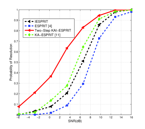
Figure 1: Probability of resolution versus SNR with $P=4$, $M=40$, $N=10$, $L=100$ runs

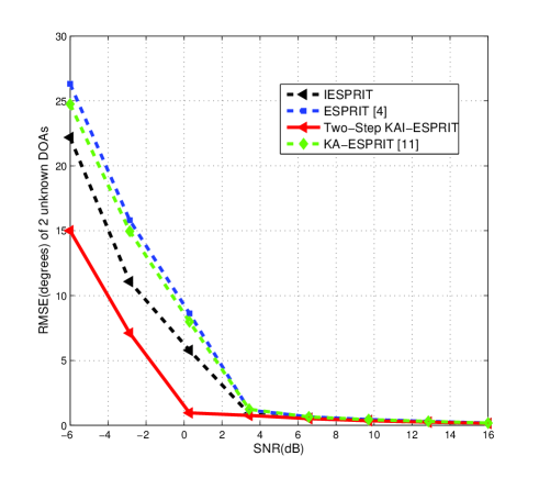
Figure 2: RMSE versus SNR with $P=4$, $M=40$, $N=10$, $L=100$ runs

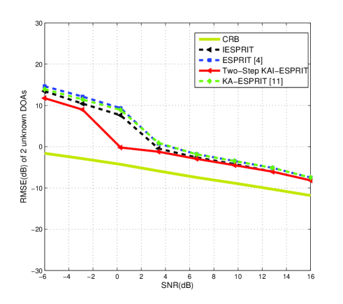
Figure 3: RMSE and the square root of CRB versus SNR with $P=4$, $M=40$, $N=10$, $L=100$ runs

VI Conclusions

We have proposed in this work the Two-Step KAI-ESPRIT algorithm which exploits prior knowledge of source signals and the structure of the covariance matrix and its perturbations. The proposed Two-Step KAI-ESPRIT algorithm can obtain significant gains in RMSE or probability of resolution performance over previously reported techniques, and has excellent potential for applications with short data records in large-scale antenna systems for wireless communications, radar and other large sensor arrays. The relatively high computational burden required, which is associated with extra matrix multiplications and the increment applied to reduce the undesirable by-products can be justified for the superior performance achieved. Future work will consider approaches to reducing computational cost.

References

- [1] H. L. Van Trees, Detection, Estimation, and Modulation, Part IV, Optimum Array Processing, John Wiley &Sons, 2002.
- [2] H. Ruan and R. C. de Lamare, “Robust Adaptive Beamforming Using a Low-Complexity Shrinkage-Based Mismatch Estimation Algorithm,” IEEE Sig. Proc. Letters., Vol. 21, No. 1, pp 60-64, 2013.
- [3] A. Elnashar, “Efficient implementation of robust adaptive beamforming based on worst-case performance optimization,” IET Signal Process., Vol. 2, No. 4, pp. 381-393, Dec 2008.
- [4] J. Zhuang and A. Manikas, “Interference cancellation beamforming robust to pointing errors,” IET Signal Process., Vol. 7, No. 2, pp. 120-127, April 2013.
- [5] L. Wang and R. C. de Lamare, “Constrained adaptive filtering algorithms based on conjugate gradient techniques for beamforming,” IET Signal Process., Vol. 4, No. 6, pp. 686-697, Feb 2010.
- [6] H. Ruan and R. C. de Lamare, “Low-Complexity Robust Adaptive Beamforming Based on Shrinkage and Cross-Correlation,” 19th International ITG Workshop on Smart Antennas, pp 1-5, March 2015.
- [7] L. L. Scharf and D. W. Tufts, “Rank reduction for modeling stationary signals,” IEEE Transactions on Acoustics, Speech and Signal Processing, vol. ASSP-35, pp. 350-355, March 1987.
- [8] A. M. Haimovich and Y. Bar-Ness, “An eigenanalysis interference canceler,” IEEE Trans. on Signal Processing, vol. 39, pp. 76-84, Jan. 1991.
- [9] D. A. Pados and S. N. Batalama ”Joint space-time auxiliary vector filtering for DS/CDMA systems with antenna arrays” IEEE Transactions on Communications, vol. 47, no. 9, pp. 1406 - 1415, 1999.
- [10] J. S. Goldstein, I. S. Reed and L. L. Scharf ”A multistage representation of the Wiener filter based on orthogonal projections” IEEE Transactions on Information Theory, vol. 44, no. 7, 1998.
- [11] Y. Hua, M. Nikpour and P. Stoica, ”Optimal reduced rank estimation and filtering,” IEEE Transactions on Signal Processing, pp. 457-469, Vol. 49, No. 3, March 2001.
- [12] M. L. Honig and J. S. Goldstein, “Adaptive reduced-rank interference suppression based on the multistage Wiener filter,” IEEE Transactions on Communications, vol. 50, no. 6, June 2002.
- [13] E. L. Santos and M. D. Zoltowski, “On Low Rank MVDR Beamforming using the Conjugate Gradient Algorithm”, Proc. IEEE International Conference on Acoustics, Speech and Signal Processing, 2004.
- [14] Q. Haoli and S.N. Batalama, “Data record-based criteria for the selection of an auxiliary vector estimator of the MMSE/MVDR filter”, IEEE Transactions on Communications, vol. 51, no. 10, Oct. 2003, pp. 1700 - 1708.
- [15] R. C. de Lamare and R. Sampaio-Neto, “Reduced-Rank Adaptive Filtering Based on Joint Iterative Optimization of Adaptive Filters”, IEEE Signal Processing Letters, Vol. 14, no. 12, December 2007.
- [16] Z. Xu and M.K. Tsatsanis, “Blind adaptive algorithms for minimum variance CDMA receivers,” IEEE Trans. Communications, vol. 49, No. 1, January 2001.
- [17] R. C. de Lamare and R. Sampaio-Neto, “Low-Complexity Variable Step-Size Mechanisms for Stochastic Gradient Algorithms in Minimum Variance CDMA Receivers”, IEEE Trans. Signal Processing, vol. 54, pp. 2302 - 2317, June 2006.
- [18] C. Xu, G. Feng and K. S. Kwak, “A Modified Constrained Constant Modulus Approach to Blind Adaptive Multiuser Detection,” IEEE Trans. Communications, vol. 49, No. 9, 2001.
- [19] Z. Xu and P. Liu, “Code-Constrained Blind Detection of CDMA Signals in Multipath Channels,” IEEE Sig. Proc. Letters, vol. 9, No. 12, December 2002.
- [20] R. C. de Lamare and R. Sampaio Neto, ”Blind Adaptive Code-Constrained Constant Modulus Algorithms for CDMA Interference Suppression in Multipath Channels”, IEEE Communications Letters, vol 9. no. 4, April, 2005.
- [21] L. Landau, R. C. de Lamare and M. Haardt, “Robust adaptive beamforming algorithms using the constrained constant modulus criterion,” IET Signal Processing, vol.8, no.5, pp.447-457, July 2014.
- [22] R. C. de Lamare, “Adaptive Reduced-Rank LCMV Beamforming Algorithms Based on Joint Iterative Optimisation of Filters”, Electronics Letters, vol. 44, no. 9, 2008.
- [23] R. C. de Lamare and R. Sampaio-Neto, “Adaptive Reduced-Rank Processing Based on Joint and Iterative Interpolation, Decimation and Filtering”, IEEE Transactions on Signal Processing, vol. 57, no. 7, July 2009, pp. 2503 - 2514.
- [24] R. C. de Lamare and Raimundo Sampaio-Neto, “Reduced-rank Interference Suppression for DS-CDMA based on Interpolated FIR Filters”, IEEE Communications Letters, vol. 9, no. 3, March 2005.
- [25] R. C. de Lamare and R. Sampaio-Neto, “Adaptive Reduced-Rank MMSE Filtering with Interpolated FIR Filters and Adaptive Interpolators”, IEEE Signal Processing Letters, vol. 12, no. 3, March, 2005.
- [26] R. C. de Lamare and R. Sampaio-Neto, “Adaptive Interference Suppression for DS-CDMA Systems based on Interpolated FIR Filters with Adaptive Interpolators in Multipath Channels”, IEEE Trans. Vehicular Technology, Vol. 56, no. 6, September 2007.
- [27] R. C. de Lamare, “Adaptive Reduced-Rank LCMV Beamforming Algorithms Based on Joint Iterative Optimisation of Filters,” Electronics Letters, 2008.
- [28] R. C. de Lamare and R. Sampaio-Neto, “Reduced-rank adaptive filtering based on joint iterative optimization of adaptive filters”, IEEE Signal Process. Lett., vol. 14, no. 12, pp. 980-983, Dec. 2007.
- [29] R. C. de Lamare, M. Haardt, and R. Sampaio-Neto, “Blind Adaptive Constrained Reduced-Rank Parameter Estimation based on Constant Modulus Design for CDMA Interference Suppression”, IEEE Transactions on Signal Processing, June 2008.
- [30] M. Yukawa, R. C. de Lamare and R. Sampaio-Neto, “Efficient Acoustic Echo Cancellation With Reduced-Rank Adaptive Filtering Based on Selective Decimation and Adaptive Interpolation,” IEEE Transactions on Audio, Speech, and Language Processing, vol.16, no. 4, pp. 696-710, May 2008.
- [31] R. C. de Lamare and R. Sampaio-Neto, “Reduced-rank space-time adaptive interference suppression with joint iterative least squares algorithms for spread-spectrum systems,” IEEE Trans. Vehi. Technol., vol. 59, no. 3, pp. 1217-1228, Mar. 2010.
- [32] R. C. de Lamare and R. Sampaio-Neto, “Adaptive reduced-rank equalization algorithms based on alternating optimization design techniques for MIMO systems,” IEEE Trans. Vehi. Technol., vol. 60, no. 6, pp. 2482-2494, Jul. 2011.
- [33] R. C. de Lamare, L. Wang, and R. Fa, “Adaptive reduced-rank LCMV beamforming algorithms based on joint iterative optimization of filters: Design and analysis,” Signal Processing, vol. 90, no. 2, pp. 640-652, Feb. 2010.
- [34] R. Fa, R. C. de Lamare, and L. Wang, “Reduced-Rank STAP Schemes for Airborne Radar Based on Switched Joint Interpolation, Decimation and Filtering Algorithm,” IEEE Transactions on Signal Processing, vol.58, no.8, Aug. 2010, pp.4182-4194.
- [35] L. Wang and R. C. de Lamare, ”Low-Complexity Adaptive Step Size Constrained Constant Modulus SG Algorithms for Blind Adaptive Beamforming”, Signal Processing, vol. 89, no. 12, December 2009, pp. 2503-2513.
- [36] L. Wang and R. C. de Lamare, “Adaptive Constrained Constant Modulus Algorithm Based on Auxiliary Vector Filtering for Beamforming,” IEEE Transactions on Signal Processing, vol. 58, no. 10, pp. 5408-5413, Oct. 2010.
- [37] L. Wang, R. C. de Lamare, M. Yukawa, ”Adaptive Reduced-Rank Constrained Constant Modulus Algorithms Based on Joint Iterative Optimization of Filters for Beamforming,” IEEE Transactions on Signal Processing, vol.58, no.6, June 2010, pp.2983-2997.
- [38] L. Wang, R. C. de Lamare and M. Yukawa, “Adaptive reduced-rank constrained constant modulus algorithms based on joint iterative optimization of filters for beamforming”, IEEE Transactions on Signal Processing, vol.58, no. 6, pp. 2983-2997, June 2010.
- [39] L. Wang and R. C. de Lamare, “Adaptive constrained constant modulus algorithm based on auxiliary vector filtering for beamforming”, IEEE Transactions on Signal Processing, vol. 58, no. 10, pp. 5408-5413, October 2010.
- [40] R. Fa and R. C. de Lamare, “Reduced-Rank STAP Algorithms using Joint Iterative Optimization of Filters,” IEEE Transactions on Aerospace and Electronic Systems, vol.47, no.3, pp.1668-1684, July 2011.
- [41] Z. Yang, R. C. de Lamare and X. Li, “L1-Regularized STAP Algorithms With a Generalized Sidelobe Canceler Architecture for Airborne Radar,” IEEE Transactions on Signal Processing, vol.60, no.2, pp.674-686, Feb. 2012.
- [42] Z. Yang, R. C. de Lamare and X. Li, “Sparsity-aware space–time adaptive processing algorithms with L1-norm regularisation for airborne radar”, IET signal processing, vol. 6, no. 5, pp. 413-423, 2012.
- [43] Neto, F.G.A.; Nascimento, V.H.; Zakharov, Y.V.; de Lamare, R.C., ”Adaptive re-weighting homotopy for sparse beamforming,” in Signal Processing Conference (EUSIPCO), 2014 Proceedings of the 22nd European , vol., no., pp.1287-1291, 1-5 Sept. 2014
- [44] Almeida Neto, F.G.; de Lamare, R.C.; Nascimento, V.H.; Zakharov, Y.V.,“Adaptive reweighting homotopy algorithms applied to beamforming,” IEEE Transactions on Aerospace and Electronic Systems, vol.51, no.3, pp.1902-1915, July 2015.
- [45] L. Wang, R. C. de Lamare and M. Haardt, “Direction finding algorithms based on joint iterative subspace optimization,” IEEE Transactions on Aerospace and Electronic Systems, vol.50, no.4, pp.2541-2553, October 2014.
- [46] S. D. Somasundaram, N. H. Parsons, P. Li and R. C. de Lamare, “Reduced-dimension robust capon beamforming using Krylov-subspace techniques,” IEEE Transactions on Aerospace and Electronic Systems, vol.51, no.1, pp.270-289, January 2015.
- [47] S. Xu and R.C de Lamare, , Distributed conjugate gradient strategies for distributed estimation over sensor networks, Sensor Signal Processing for Defense SSPD, September 2012.
- [48] S. Xu, R. C. de Lamare, H. V. Poor, “Distributed Estimation Over Sensor Networks Based on Distributed Conjugate Gradient Strategies”, IET Signal Processing, 2016 (to appear).
- [49] S. Xu, R. C. de Lamare and H. V. Poor, Distributed Compressed Estimation Based on Compressive Sensing, IEEE Signal Processing letters, vol. 22, no. 9, September 2014.
- [50] S. Xu, R. C. de Lamare and H. V. Poor, “Distributed reduced-rank estimation based on joint iterative optimization in sensor networks,” in Proceedings of the 22nd European Signal Processing Conference (EUSIPCO), pp.2360-2364, 1-5, Sept. 2014
- [51] S. Xu, R. C. de Lamare and H. V. Poor, “Adaptive link selection strategies for distributed estimation in diffusion wireless networks,” in Proc. IEEE International Conference onAcoustics, Speech and Signal Processing (ICASSP), , vol., no., pp.5402-5405, 26-31 May 2013.
- [52] S. Xu, R. C. de Lamare and H. V. Poor, “Dynamic topology adaptation for distributed estimation in smart grids,” in Computational Advances in Multi-Sensor Adaptive Processing (CAMSAP), 2013 IEEE 5th International Workshop on , vol., no., pp.420-423, 15-18 Dec. 2013.
- [53] S. Xu, R. C. de Lamare and H. V. Poor, “Adaptive Link Selection Algorithms for Distributed Estimation”, EURASIP Journal on Advances in Signal Processing, 2015.
- [54] N. Song, R. C. de Lamare, M. Haardt, and M. Wolf, “Adaptive Widely Linear Reduced-Rank Interference Suppression based on the Multi-Stage Wiener Filter,” IEEE Transactions on Signal Processing, vol. 60, no. 8, 2012.
- [55] N. Song, W. U. Alokozai, R. C. de Lamare and M. Haardt, “Adaptive Widely Linear Reduced-Rank Beamforming Based on Joint Iterative Optimization,” IEEE Signal Processing Letters, vol.21, no.3, pp. 265-269, March 2014.
- [56] R.C. de Lamare, R. Sampaio-Neto and M. Haardt, ”Blind Adaptive Constrained Constant-Modulus Reduced-Rank Interference Suppression Algorithms Based on Interpolation and Switched Decimation,” IEEE Trans. on Signal Processing, vol.59, no.2, pp.681-695, Feb. 2011.
- [57] Y. Cai, R. C. de Lamare, “Adaptive Linear Minimum BER Reduced-Rank Interference Suppression Algorithms Based on Joint and Iterative Optimization of Filters,” IEEE Communications Letters, vol.17, no.4, pp.633-636, April 2013.
- [58] R. C. de Lamare and R. Sampaio-Neto, “Sparsity-Aware Adaptive Algorithms Based on Alternating Optimization and Shrinkage,” IEEE Signal Processing Letters, vol.21, no.2, pp.225,229, Feb. 2014.
- [59] R. C. de Lamare, “Massive MIMO Systems: Signal Processing Challenges and Future Trends”, Radio Science Bulletin, December 2013.
- [60] W. Zhang, H. Ren, C. Pan, M. Chen, R. C. de Lamare, B. Du and J. Dai, “Large-Scale Antenna Systems With UL/DL Hardware Mismatch: Achievable Rates Analysis and Calibration”, IEEE Trans. Commun., vol.63, no.4, pp. 1216-1229, April 2015.
- [61] R. Schmidt, ”Multiple emitter location and signal parameter estimation” IEEE Trans on Antennas and Propagation, vol.34, No.3, Mar 1986, pp 276-280.
- [62] A. J. Barabell, “Improving the resolution performance of eigenstructure-based direction-finding algorithms,” in Proc. ICASSP, Boston, MA, Apr. 1983, pp. 336–339.
- [63] R. Roy and T. Kailath, ”Estimation of signal parameters via rotational invariance techniques”, IEEE Trans. Acoust., Speech., Signal Processing, vol. 37, July 1989, pp 984-995.
- [64] J. Steinwandt, R. C. de Lamare and M. Haardt, ”Beamspace direction finding based on the conjugate gradient and the auxiliary vector filtering algorithms”, Signal Processing, vol. 93, no. 4, April 2013, pp. 641-651.
- [65] L. Wang, R. C. de Lamare and M. Haardt, ”Direction finding algorithms based on joint iterative subspace optimization,” IEEE Transactions on Aerospace and Electronic Systems, vol. 50, no. 4, pp. 2541-2553, October 2014.
- [66] L. Qiu, Y. Cai, R. C. de Lamare and M. Zhao, “Reduced-Rank DOA Estimation Algorithms Based on Alternating Low-Rank Decomposition,” IEEE Signal Processing Letters, vol. 23, no. 5, pp. 565-569, May 2016.
- [67] X. Mestre, “Improved estimation of eigenvalues and eigenvectors of covariance matrices using their sample estimates,” IEEE Trans. Inf. Theory, vol. 54, no. 11, pp. 5113–5129, Nov. 2008.
- [68] X. Mestre and M. A. Lagunas, “Modified subspace algorithms for DOA estimation with large arrays,” IEEE Trans. Signal Process., vol. 56, no. 2, pp. 598–614, Feb. 2008.
- [69] P. Vallet, P. Loubaton, and X. Mestre, “Improved subspace estimation for multivariate observations of high dimension: the deterministic signal case”, IEEE Trans. Inf. Theory, vol. 58, no. 2, pp. 1043–1068, Feb. 2012.
- [70] J. Steinwandt, R. C. de Lamare and M. Haardt, “Knowledge-aided direction finding based on Unitary ESPRIT,” 2011 Conference Record of the Forty Fifth Asilomar Conference on Signals, Systems and Computers (ASILOMAR), Pacific Grove, CA, 2011, pp. 613-617.
- [71] G. Bouleux, P. Stoica, and R. Boyer, ”An optimal prior knowledge-based DOA estimation method,” in 17th European Signal Processing Conference (EUSIPCO), Aug. 2009, pp. 869-873.
- [72] M. Shaghaghi and S. A. Vorobyov, ”Iterative root-MUSIC algorithm for DOA estimation”, 5th IEEE international Workshop on Computational Advances in Multisensor Adaptive Processing (CAMSAP), 2013.
- [73] M. Shaghaghi and S. A. Vorobyov, ”Subspace leakage analysis and improved DOA estimation with small sample size”, IEEE Trans. Signal Process., vol. 63, no.12, pp 3251-3265, Jun.2015.
- [74] P. Stoica and A. Nehorai, “Performance study of conditional and unconditional direction-of-arrival estimation,” IEEE Trans. Acoust., Speech, Signal Process., vol. 38, no. 10, pp. 1783–1795, Oct. 1990.
- [75] P. Stoica, J. Li, X. Zhu, and J. R. Guerci, ”On using a priori knowledge in space-time adaptive processing,” IEEE Transactions on Signal Processing, vol. 56, no. 6, pp. 2598-2602, June 2008.
- [76] P.Stoica and A.B.Gershman, ”Maximum-likelihood doa estimation by data-supported grid search”, IEEE Signal Processing Letters, vol. 6, no. 10, pp. 273- 275, Oct 1999.
- [77] P.Stoica and Arye Nehorai, ”MUSIC, maximum Likelihood, and Cramer-Rao Bound”, IEEE Transactions on Acoustics, Speech and Signal Processing, vol. 37, no. 5, pp. 720- 741, May 1989.
- [78] R.Grover, D.A.Pados, M.J. Medley,Subspace direction finding with an auxiliary-vector basis,IEEE Transactions on Signal Processing, 55 (2) (2007) pp.758–763.
- [79] H.Semira, H.Belkacemi, S.Marcos, High-resolution source localiza- tion algorithm based on the conjugate gradient, EURASIP Journa lon Advances in Signal Processing, 2007(2)(2007)1–9.