On the Viability of the Intermediate Inflation Scenario with $F(T)$ Gravity

Abstract

We study the intermediate inflation scenario in the context of $F(T)$ gravity, and we examine it’s viability by calculating the power spectrum of the primordial curvature perturbations and the corresponding spectral index. As we demonstrate, it is possible for the resulting spectral index to be compatible with the observational data and we investigate the parameter space in order to see when the compatibility with data is possible.

I Introduction

An alternative theory to Einstein-Hilbert gravity is $F(T)$ gravity, where the fundamental quantity that is used is the torsion $T$ corresponding to the Weitzenböck connection  Hehl:1976kj ; Hayashi:1979qx ; Cai:2015emx ; Flanagan:2007dc ; Maluf:2013gaa ; Ferraro:2008ey , instead of the Ricci scalar corresponding to the Levi-Civita connection. In general, modified gravity models of teleparallelism, in which case the theory is built by using a appropriately chosen function of the torsion $T$, can explain various cosmological eras of our Universe, for example the late-time acceleration issue in the context of $F(T)$ gravity was studied in Refs. Bamba:2013jqa ; Bengochea:2008gz ; Linder:2010py ; Geng:2011aj ; Otalora:2013tba ; Chattopadhyay:2012eu ; Dent:2011zz ; Yang:2010hw ; Bamba:2010wb ; Capozziello:2011hj ; Geng:2011ka ; Farajollahi:2011af ; Cardone:2012xq ; Bahamonde:2015zma , while inflationary and bouncing scenarios in relation with cosmological perturbation scenarios were studied in Refs. Cai:2011tc ; Chen:2010va ; Izumi:2012qj ; Nashed:2014lva ; Hanafy:2014bsa ; Hanafy:2014ica ; Ferraro:2006jd . Moreover, special cosmological solutions where found in Refs. Rodrigues:2012qua ; Li:2013xea and special metric solutions or astrophysical objects studies where performed in Refs. Capozziello:2012zj ; Paliathanasis:2014iva ; Gonzalez:2011dr ; Bohmer:2011si ; Nashed:2013bfa ; Ruggiero:2015oka , and in addition thermodynamical issues were addressed in Bamba:2012vg ; Bamba:2010wb ; Karami:2012fu . This research stream renders $F(T)$ gravity an important alternative to Einstein-Hilbert gravity. To this end, the purpose of this paper is to investigate if a quite popular inflation scenario, and specifically the intermediate inflation scenario Barrow:1990td ; Barrow:1993zq ; Rezazadeh:2014fwa ; Barrow:2006dh ; Barrow:2014fsa ; Herrera:2014mca ; Jamil:2013nca ; Herrera:2010vv ; Rendall:2005if , can produce a nearly scale invariant power spectrum, compatible with the observational data in the context of $F(T)$ gravity. For a relevant work on intermediate inflation in the context of $F(T)$ gravity, see Jamil:2013nca . We shall investigate which $F(T)$ gravity can approximately realize the intermediate inflation scenario, emphasizing at early cosmic times, and we shall calculate the evolution of scalar perturbations and the corresponding spectral index. As we shall demonstrate, the intermediate inflation scenario in the context of $F(T)$ gravity, produces a nearly scale invariant power spectrum, with a spectral index compatible with the latest (2015) observational data, coming from the Planck collaboration Ade:2015lrj . In addition, we perform an analysis of the free parameters space and we investigate for which values of the parameters, compatibility with the Planck data can be achieved.

This paper is organized as follows: In section II we present in brief some essential features of the $F(T)$ gravity and also the necessary formalism for the sections to follow. In section III we investigate which $F(T)$ gravity can approximately generate the intermediate inflation scenario, emphasizing at early times, and we calculate the power spectrum of primordial perturbations. In addition we calculate the spectral index and we discuss its compatibility with the observational data. In section IV we perform an analysis of the free parameters space and we discuss how the compatibility with the observational data can be achieved for various values of the parameters. Finally, the conclusions follow at the end of the paper.

II Essential Features of $F(T)$ Gravity

For the $F(T)$ gravity formalism, the orthonormal tetrad components $e_{A}(x^{\mu})$ are used, which are very common in teleparallelism theories, where the index $A$ is $A=0,1,2,3$, on the tangent space of each spacetime point $x^{\mu}$ of the spacetime manifold. Effectively, the tetrads $e_{A}^{\mu}$ form the tangent vector of the spacetime manifold. The tetrad components are related to the spacetime metric $g^{\mu\nu}$ as follows $g_{\mu\nu}=\eta_{AB}e^{A}_{\mu}e^{B}_{\nu}$. The torsion $T^{\rho}_{\verb| |\mu\nu}$ and the contorsion $K^{\mu\nu}_{\verb||\rho}$ tensors, are defined as follows,

$$T^{\rho}_{\ \mu\nu}\equiv e^{\rho}_{A}\left(\partial_{\mu}e^{A}_{\nu}-\partial_{\nu}e^{A}_{\mu}\right)\,,$$ (1)

$$K^{\mu\nu}_{\ \ \rho}\equiv-\frac{1}{2}\left(T^{\mu\nu}_{\ \ \rho}-T^{\nu\mu}_{\ \ \rho}-T_{\rho}^{\ \ \mu\nu}\right)\,.$$

In addition, the torsion scalar $T$ is defined as follows, Hayashi:1979qx

$$T\equiv S_{\rho}^{\ \mu\nu}T^{\rho}_{\ \mu\nu}\,,\quad S_{\rho}^{\ \mu\nu}\equiv\frac{1}{2}\left(K^{\mu\nu}_{\ \ \rho}+\delta^{\mu}_{\rho}T^{\alpha\nu}_{\ \ \alpha}-\delta^{\nu}_{\rho}T^{\alpha\mu}_{\ \ \alpha}\right)\,.$$ (2)

In effect, the $F(T)$ modified teleparallel gravity action is equal to,

$$S=\int d^{4}x|e|\left[\frac{F(T)}{2{\kappa}^{2}}+{\mathcal{L}}_{\mathrm{matter}}\right]\,,$$ (3)

where $|e|=\det\left(e^{A}_{\mu}\right)=\sqrt{-g}$. By varying the gravitational action of Eq. (3), with respect to the vierbein $e_{A}^{\mu}$, we get,

$$\frac{1}{e}\partial_{\mu}\left(eS_{A}^{\ \mu\nu}\right)F^{\prime}-e_{A}^{\lambda}T^{\rho}_{\ \mu\lambda}S_{\rho}^{\ \nu\mu}F^{\prime}$$ (4)

$$+S_{A}^{\ \mu\nu}\partial_{\mu}Tf^{\prime\prime}+\frac{1}{4}e_{A}^{\nu}F=\frac{{\kappa}^{2}}{2}e_{A}^{\rho}T_{(\mathrm{matter}\,\rho}^{\ \ \ \ \ \nu}\,.$$

By considering a flat FRW metric with line element,

$$ds^{2}=-dt^{2}+a(t)^{2}\sum_{i=1,2,3}\left(dx^{i}\right)^{2}\,,$$ (5)

then we find that the tetrad components are equal to, $e^{A}_{\mu}=\mathrm{diag}\left(1,a,a,a\right)$, which implies that $g_{\mu\nu}=\mathrm{diag}\left(1,-a^{2},-a^{2},-a^{2}\right)$. In effect, the torsion scalar $T$ is equal to, $T=-6H^{2}$, and in addition, for the flat FRW metric, Eq. (4) becomes,

$$\frac{3}{\kappa^{2}}H^{2}=\rho_{\mathrm{matter}}+\rho_{\mathrm{DE}}\,,\quad\frac{1}{\kappa^{2}}\left(H^{2}+\dot{H}\right)=p_{\mathrm{matter}}+p_{\mathrm{DE}}\,,$$ (6)

where,

$$\rho_{\mathrm{DE}}=\frac{1}{2{\kappa}^{2}}\left(-T-f+2Tf^{\prime}\right)\,,$$ (7)

$$p_{\mathrm{DE}}=-\frac{1}{2{\kappa}^{2}}\left(\left(4-4f^{\prime}-8TF^{\prime\prime}\right)\dot{H}-T-f+2Tf^{\prime}\right)\,,$$

and the prime denotes differentiation with respect to $T$. The energy density $\rho_{\mathrm{DE}}$ and the pressure $p_{\mathrm{DE}}$ appearing in Eq. (7), satisfy the usual continuity equation

$$0=\dot{\rho}_{\mathrm{DE}}+3H\left(\rho_{\mathrm{DE}}+p_{\mathrm{DE}}\right)\,,$$ (8)

and the same applies for the energy density $\rho_{\mathrm{matter}}$ and for the pressure $p_{\mathrm{matter}}$, which correspond to the perfect matter fluids which are present. In the purely vacuum case we have $\rho_{\mathrm{matter}}=p_{\mathrm{matter}}=0$, and the first equation in Eq. (6) becomes,

$$0=-F+2TF^{\prime}\,,\quad 0=F^{\prime}+2TF^{\prime\prime}\,,$$ (9)

where we used the fact that $T=-6H^{2}$. In the following sections we shall use the above formalism and we shall apply the above reconstruction technique in order to find the $F(T)$ gravity which realizes the intermediate inflation scenario.

III Intermediate Inflation and Evolution of Perturbations in $F(T)=T+f(T)$ Gravity

As we already mentioned, in this paper we shall be interested in the intermediate inflation scenario, which is quite popular in the literature, see for example Barrow:1990td ; Barrow:1993zq ; Rezazadeh:2014fwa ; Barrow:2006dh ; Barrow:2014fsa ; Herrera:2014mca ; Jamil:2013nca ; Herrera:2010vv ; Rendall:2005if . In the standard approach of intermediate inflation, it was worked out in the context of scalar-tensor gravity Barrow:1993zq ; Rezazadeh:2014fwa ; Barrow:2006dh ; Barrow:2014fsa , and its viability as a cosmological theory of the early Universe was examined in Refs. Barrow:2006dh ; Barrow:2014fsa ; Herrera:2014mca . We shall investigate whether this model of inflation is viable in the context of $F(T)$ gravity. The intermediate inflation scale factor and the Hubble rate are Barrow:1990td ,

$$a(t)=e^{A\,t^{n}},\,\,\,H(t)=Ant^{n-1}\,,$$ (10)

where $0<n<1$ and also $A>0$. The calculation of the evolution of primordial perturbations in the context of $F(T)$ gravity, can be found in various texts in the literature Cai:2011tc ; Chen:2010va ; Izumi:2012qj ; Nashed:2014lva ; Hanafy:2014bsa ; Hanafy:2014ica , and we adopt the formalism and notation of Ref. Cai:2011tc . For a general approach applicable to various cosmological contexts, see for example Brandenberger:2016vhg . We shall be interested in the longitudinal gauge, and therefore we consider only scalar-type metric fluctuations. In effect, the perturbed metric has the following form,

$$\mathrm{d}s^{2}=(1+2\Phi)\mathrm{d}t^{2}-a(t)^{2}(1-2\Psi)\sum_{i}\mathrm{d}x^{2}_{i}\,.$$ (11)

It is conceivable that the scalar fluctuations of the metric are quantified by the scalar functions $\Phi$ and $\Psi$. The leading order perturbation of the torsion scalar can be expressed in terms of the functions $\Phi$ and $\Psi$ as follows,

$$\delta T=12H(\dot{\Phi}+H\Psi)\,,$$ (12)

where $H$ stands for the Hubble rate. In effect, by using the formalism and the equations of motion of the previous section, we find the following perturbation equations of the $F(T)$ gravity Cai:2011tc , which correspond to the perturbed metric (11),

$$(1+f_{,T})\frac{\nabla^{2}}{a^{2}}\Psi-3(1+f_{,T})H\dot{\Psi}-3(1+f_{,T})H^{2}\Phi$$ (13)

$$+36f_{,TT}H^{3}(\dot{\Psi}+H\Phi)=4\pi G\delta\rho\,,$$

$$(1+f_{,T}-12H^{2}f_{,TT})(\dot{\Psi}+H\Phi)=4\pi G\delta q\,,$$

$$(1+f_{,T})(\Psi-\Phi)=8\pi G\delta s\,,$$

$$(1+f_{,T}-12H^{2}f_{,TT})\ddot{\Psi}+3H(1+f_{,T}$$

$$-12H^{2}f_{,TT}-12\dot{H}f_{,TT}+48H^{2}\dot{H}f_{,TTT})\dot{\Psi}$$

$$+\Big{[}3H^{2}(1+f_{,T}-12H^{2}f_{,TT})+2\dot{H}(1+f_{,T}-30H^{2}f_{,TT}$$

$$+72H^{4}f_{,TTT})\Big{]}\Phi+\frac{1+f_{,T}}{2a^{2}}\nabla^{2}(\Psi-\Phi)=4\pi G\delta p\,,$$

with $f_{,T}$, standing for $\partial_{T}f(T)$, and the derivatives $f_{,TT}$ and $f_{,TTT}$ can be found accordingly. Moreover, the functions $\delta p$, $\delta\rho$, $\delta q$, $\delta s$, denote the fluctuations of the total pressure, of the total energy density and of the fluid velocity and of the anisotropic stress respectively. Assuming that a canonical scalar field represents the matter fluid present, which has a potential $V(\phi)$, we get the following equations,

$$\delta\rho=\dot{\phi}(\delta\dot{\phi}-\dot{\phi}\Phi)+V_{,\phi}\delta\phi\,,$$ (14)

$$\delta q=\dot{\phi}\delta\phi\,,$$

$$\delta s=0\,,$$

$$\delta p=\dot{\phi}(\delta\dot{\phi}-\dot{\phi}\Phi)-V_{,\phi}\delta\phi\,.$$

In view of the above equations, it was shown in Ref. Cai:2011tc , that the relation $\Psi=\Phi$ holds true, and in addition, the scalar fluctuation $\delta\phi$, uniquely determines the gravitational potential $\Phi$. In effect, the $f(T)$ gravity minimally coupled to a scalar field has one degree of freedom. With regard to the evolution of the scalar perturbations, the following equation determine how these evolve in time Cai:2011tc ,

$$\ddot{\Phi}_{k}+\alpha\dot{\Phi}_{k}+\mu^{2}\Phi_{k}+c_{s}^{2}\frac{k^{2}}{a^{2}}\Phi_{k}=0\,,$$ (15)

with $\Phi_{k}$ being the scalar Fourier mode of the potential $\Phi$, and in addition, the functions $c_{s}^{2}$, $\alpha$ and $\mu^{2}$ are the the speed of sound parameter, the frictional term and the effective mass respectively, corresponding to the scalar potential $\Phi$. In detail, the latter functions are equal to,

$$\alpha=7H+\frac{2V_{,\phi}}{\dot{\phi}}-\frac{36H\dot{H}(f_{,TT}-4H^{2}f_{,TTT})}{1+f_{,T}-12H^{2}f_{,TT}}\,,$$ (16)

$$\mu^{2}=6H^{2}+2\dot{H}+\frac{2HV_{,\phi}}{\dot{\phi}}-\frac{36H^{2}\dot{H}(f_{,TT}-4H^{2}f_{,TTT})}{1+f_{,T}-12H^{2}f_{,TT}}\,,$$

$$c_{s}^{2}=\frac{1+f_{,T}}{1+f_{,T}-12H^{2}f_{,TT}}\,.$$

The equation of motion for the canonical scalar field is,

$$\ddot{\phi}+3H\dot{\phi}+V_{,\phi}=0\,,$$ (17)

and thus by rewriting the $f(T)$ gravity equation of motion as follows,

$$(a+f_{,T}-12H^{2}f_{,TT})\dot{H}=-4\pi G\dot{\phi}^{2}\,,$$ (18)

the master equation that determines the evolution of scalar perturbations is,

$$\ddot{\Phi}_{k}+\left(H-\frac{\ddot{H}}{\dot{H}}\right)\dot{\Phi}_{k}+\left(2\dot{H}-\frac{H\ddot{H}}{\dot{H}}\right)\Phi_{k}+\frac{c_{s}^{2}k^{2}}{a^{2}}\Phi_{k}=0\,.$$ (19)

As it can be seen from the structure of Eq. (19), it is identical to the Einstein-Hilbert master equation, apart from the appearance of the speed of sound parameter.

A physical quantity that can adequately quantify any cosmological inhomogeneities, is the comoving curvature fluctuation, which we denote as $\zeta$, which in the case at hand is equal to,

$$\zeta=\Phi-\frac{H}{\dot{H}}\left(\dot{\Phi}+H\Phi\right)\,.$$ (20)

The comoving curvature fluctuation is gauge invariant and it simplifies significantly the calculation of the spectral index. We also introduce the quantity $v$ which is defined as follows,

$$v=z\zeta\,,$$ (21)

where $z$ stands for,

$$z=a\sqrt{2\epsilon}\,,$$ (22)

and also $\epsilon$ is the first slow-roll index $\epsilon=-\frac{\dot{H}}{H^{2}}$. In terms of the new variables $v$ and $z$, the master equation that determines the evolution of primordial curvature perturbations becomes Cai:2011tc ,

$$v_{k}^{\prime\prime}+\left(c_{s}^{2}k^{2}-\frac{z^{\prime\prime}}{z}\right)v_{k}=0\,,$$ (23)

where the sound speed parameter appears in Eq. (16). Note here that the “prime” in Eq. (23) denotes differentiation with respect to the conformal time $\tau$, which in terms of the cosmic time $t$ is defined as follows,

$$\tau=\int\mathrm{d}t\frac{1}{a}\,.$$ (24)

We need to note that the $f(T)$ gravity affects the evolution of the primordial curvature perturbations (23) via the speed of sound parameter $c_{s}$, and for the flat FRW background of Eq. (5), the $f(T)$ gravity first Friedmann equation becomes,

$$H^{2}=-\frac{f(T)}{6}-2f_{,T}H^{2}\,,$$ (25)

and since $T=-6H^{2}$, for the intermediate inflation case (10) we obtain,

$$T=-6A^{2}n^{2}t^{2n-2}\,.$$ (26)

By solving the above equation with respect to the cosmic time $t$, we obtain the function $t(T)$, which is,

$$t(T)=6^{-\frac{1}{2n-2}}\left(-\frac{T}{A^{2}n^{2}}\right)^{\frac{1}{2n-2}}\,.$$ (27)

By combining Eqs. (25) and (27), we obtain the approximate form of the $f(T)$ gravity which realizes the intermediate inflation scenario, which is,

$$f(T)=c_{1}T^{\frac{An}{2}}-\frac{T}{2\left(1-\frac{An}{2}\right)}\,,$$ (28)

with $c_{1}$ being an arbitrary integration constant, and hence the total $F(T)$ gravity is $F(T)=T+f(T)$. At this point we shall express all the quantities as function of the conformal time $\tau$, however in the case at hand, certain simplifications can be made. Particularly, since we are interested for the inflationary era, this means that we are interested in the early-time era, so the cosmic time variable takes small values. In effect, the exponential $e^{At^{n}}$ for small values of $t$ can be approximated as $e^{At^{n}}\sim 1$, and therefore we may identify the cosmic time $t$ with the conformal time $\tau$ (see relation (24)), that is $\tau\sim t$. In effect, the function $z(t)$ for the intermediate $f(T)$ inflation reads,

$$z(t)=\sqrt{\frac{2(1-n)t^{-n}}{An}}\,,$$ (29)

and moreover, by using Eq. (28) the sound speed parameter is equal to,

$$c_{s}^{2}(t)=\frac{A\,c_{1}\,n6^{\frac{An}{2}}(An-2)\left(-A^{2}n^{2}t^{2n-2}\right)^{\frac{An}{2}}}{2(An-1)S(t)}$$ (30)

$$-\frac{12A^{2}n^{2}(An-1)t^{2n-2}}{2(An-1)S(t)}\,,$$

where $S(t)$ is,

$$S(t)=\Big{(}c_{1}6^{\frac{An}{2}}(An-2)\left(-A^{2}n^{2}t^{2n-2}\right)^{\frac{An}{2}}$$ (31)

$$-6A^{2}n^{2}t^{2n-2}\Big{)}\,.$$

Due to the fact that the dominant term in the expression of Eq. (30) is $\sim t^{2n-2}$, we may approximate the sound speed parameter as $c_{s}^{2}\simeq 1$. In effect, the master equation describing the evolution of the perturbations can be written as follows,

$$v^{\prime\prime}_{k}(t)+\left(k^{2}-\frac{\left(\frac{n}{2}+1\right)n}{2t^{2}}\right)v_{k}(t)=0\,,$$ (32)

which has the following solution,

$$v_{k}(t)=C_{1}\sqrt{t}J_{\frac{n+1}{2}}(kt)+C_{2}\sqrt{t}Y_{\frac{n+1}{2}}(kt)\,,$$ (33)

with $J_{n}(z)$ and $Y_{n}(z)$ being the Bessel functions of first and second kind respectively, and in addition $C_{1}$ and $C_{2}$ are arbitrary integration constants. The expression of Eq. (33) can be simplified for small values of the Bessel functions arguments, so we get the simplified result for $v_{k}(t)$, which is,

$$v_{k}(t)=\frac{\text{C1}\sqrt{t}(kt)^{n/2}\left(2^{\frac{1}{2}(-n-1)}\sqrt{kt}\right)}{\Gamma\left(\frac{n+1}{2}+1\right)}$$ (34)

$$+\text{C2}\sqrt{t}\Big{(}-\frac{2^{\frac{n}{2}+\frac{1}{2}}\Gamma\left(\frac{n+1}{2}\right)(kt)^{-\frac{n}{2}-\frac{1}{2}}}{\pi}$$

$$-\frac{2^{-\frac{n}{2}-\frac{1}{2}}\cos\left(\frac{1}{2}\pi(n+1)\right)\Gamma\left(\frac{1}{2}(-n-1)\right)(kt)^{\frac{n}{2}+\frac{1}{2}}}{\pi}\Big{)}\,,$$

and by keeping only leading order terms we acquire,

$$v_{k}(t)=\frac{C_{2}\sqrt{t}\left(2^{\frac{n}{2}+\frac{1}{2}}\Gamma\left(\frac{n+1}{2}\right)(kt)^{-\frac{n}{2}-\frac{1}{2}}\right)}{\pi}\,.$$ (35)

At this point we proceed in calculating the power spectrum of the primordial curvature perturbations, which in terms of the functions $v_{k}$ and $z$ is defined as follows,

$$\mathcal{P}_{\zeta}=\frac{k^{3}}{2\pi^{2}}|\frac{v_{k}}{z}|_{k=aH}^{2}\,,$$ (36)

and note that it must be evaluated at the horizon crossing, which occurs when $k=aH$, where $k$ is the wavenumber of each primordial mode. In order to find an analytical expression for the power spectrum, we need to express the quantity $|\frac{v_{k}}{z}|^{2}$ as a function of the wavenumber $k$. Note that, firstly, we already have the function $v_{k}(t)$, which we calculated the resulting expression in Eq. (35), however, the parameter $C_{2}$ is also $k$-dependent. This $k$-dependence of $C_{2}$ can be determined by assuming some initial conditions for the function $v_{k}(t_{0})$. Particularly we assume that it originates from a Bunch-Davies vacuum, and hence we have $v_{k}\simeq\frac{e^{-ikt}}{\sqrt{2k}}$. In effect the constant $C_{2}$ as a function of the wavenumber is,

$$C_{4}\simeq\frac{\pi 2^{-\frac{n}{2}-\frac{1}{2}}k^{n/2}t^{n/2}}{\Gamma\left(\frac{n+1}{2}\right)}\,.$$ (37)

We need to note that the assumption of the Bunch-Davies vacuum is an assumption based on the fact that the intermediate inflation scenario is an inflationary scenario. The Bunch-Davies vacuum assumption is based on the fact that the initial state corresponds to an era that the curvature does not affect the fluctuations. It is possible though that before the inflationary era, another scenario might occur, like for example a bouncing phase ref1 , so in effect the Bunch-Davies assumption would be inapplicable. Therefore, one should adopt the approach of Refs. ref12 ; ref2 in order to find the correct approximation for the initial state. In fact, as it shown in ref3 , in some cases the intermediate inflation scenario is identical with the expanding phase of a singular bounce. Then, the considerations of Refs. ref12 ; ref2 might be compelling. However, for the purposes of this paper we assume that the initial state remains a Bunch-Davies vacuum state and we defer this non-trivial task to a future work.

Another quantity that has an implicit $k$-dependence is the cosmic time in both Eqs. (35) and (37). In order to find the $k$-dependence, recall that the power spectrum is evaluated at the horizon crossing, where the equation $k=aH$, and since $a\sim 1$ at early times, we have,

$$t\simeq\frac{k^{\frac{1}{n-1}}}{(An)^{\frac{1}{n-1}}}\,.$$ (38)

Hence, by combining Eqs. (29), (35), (37) and (38), the resulting power spectrum of Eq. (36) is equal to,

$$\mathcal{P}_{\zeta}\simeq\frac{\left(n^{1-\frac{n}{n-1}}A^{1-\frac{n}{n-1}}\right)k^{\frac{1}{n-1}+3}}{4\pi^{2}(1-n)}\,.$$ (39)

Obviously, the power spectrum is not scale invariant, however, as we show in the next section, it can be compatible with the Planck data, since a nearly scale invariant spectrum is produced for specifically chosen values of the parameter $n$.

III.1 Comparison with Planck 2015 Data and Analysis of the Parameter Space

Having the expression for the power spectrum of primordial curvature perturbations at hand, namely Eq. (39), we can calculate the spectral index straightforwardly, by using the following relation,

$$n_{s}-1=\frac{\mathrm{d}\ln\mathcal{P}_{\zeta}}{\mathrm{d}\ln k}\,.$$ (40)

Therefore, for the power spectrum of Eq. (39), the spectral index reads,

$$n_{s}=\frac{1}{n-1}+4\,,$$ (41)

and now we investigate whether this spectral index can be compatible with the 2015 observational data of the Planck collaboration Ade:2015lrj , in which case the spectral index is constrained as follows,

$$n_{s}=0.9644\pm 0.0049\,.$$ (42)

In effect, a spectral index $n_{s}$ that takes values in the interval $n_{s}=[0.9595,0.9693]$ can be considered compatible with the Planck constraints (42).

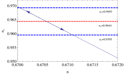
Figure 1: The spectral index $n_{s}=\frac{1}{n-1}+4$ as a function of the parameter $n$. The curve with arrows indicates the values of $n$ for which the spectral index is compatible with the Planck 2015 constraints on the spectral index.

In Fig. 1, we have plotted the spectral index $n_{s}=\frac{1}{n-1}+4$, as a function of $n$, and as it can be seen, the allowed range of $n$ is indicated by the arrows. The upper dashed line (red in online version) indicates the highest value of the spectral index that it is allowed, namely $n_{s}=0.9693$, while the lower dashed line (red in online version) indicates the lowest allowed value of the spectral index, namely $n_{s}=0.9595$. The middle dashed (red in online version) line corresponds to $n_{s}=0.9644$. Hence if $n$ is chosen to take values in the range $n=[0.67,0.6711]$, then the spectral index $n_{s}$ takes values in the interval $n_{s}=[0.9595,0.9693]$, and hence it is compatible with the Planck data. In conclusion, for the $F(T)$ gravity description of the intermediate inflation scenario, the resulting spectral index depends only on one parameter $n$, that appears in the scale factor of the intermediate inflation scenario, and it can be compatible with the Planck 2015 observational data, if $n$ takes values in the interval $n=[0.67,0.6711]$.

III.2 Discussion on the Scalar-to-tensor Ratio

We now discuss the calculation of the scalar-to-tensor ratio, which in the case at hand it will prove a non-trivial task. Consider the perturbation of the flat FRW metric,

$$\mathrm{d}s^{2}=a(\tau)^{2}\left(-\mathrm{d}\tau^{2}+(\delta_{ij}+h_{ij}\mathrm{d}x^{i}\mathrm{d}x^{j})\right)\,,$$ (43)

where the tensor perturbation $h_{ij}$ is real, transverse and traceless, that is, $h_{ij}=h_{ji}$, $h_{ii}=0$ and $h_{ij,j}=0$. The calculation of the amplitude of the tensor modes can be done by using standard approaches, see for example Chen:2010va ; ref4 , so the resulting master differential equation that governs the evolution of the tensor perturbations is,

$$\left(\ddot{h}_{ij}+3H\dot{h}_{ij}-\frac{\nabla^{2}}{a^{2}}h_{ij}\right)-\frac{12H\dot{H}f_{,TT}}{1+f_{,T}}\dot{h}_{ij}=0\,.$$ (44)

By expanding the tensor perturbation $h_{ij}$ in Fourier modes, one can calculate the evolution of each tensor Fourier mode. However, for the case at hand this is a highly non-trivial task, and it is very difficult to obtain analytic results even by taking the small $t$ limit. This is due to the presence of the last term in Eq. (44), which contains the derivatives of the function $f(T)$, which in our case, by using Eq. (28), the last term reads,

$$-\frac{12H\dot{H}f_{,TT}}{1+f_{,T}}\dot{h}_{ij}=$$ (45)

$$\left(\frac{6A^{3}C_{1}(n-1)n^{3}(An-2)^{2}t^{2n-3}T^{\frac{An}{2}-1}}{AC_{1}n(An-2)T^{\frac{An}{2}}+2T(An-1)}\right)\dot{h}_{ij}\,,$$

and by using Eq. (26), we can express it in terms of the cosmic time (recall that the cosmic and the conformal time are equivalent in the small $t$ limit in our case, see Eq. (24), with $a\sim 1$),

$$-\frac{12H\dot{H}f_{,TT}}{1+f_{,T}}\dot{h}_{ij}=$$ (46)

$$\left(\frac{(n-1)t(An-2)^{2}}{\frac{An2^{2-\frac{An}{2}}3^{1-\frac{An}{2}}(An-1)t^{2n}\left(A^{2}n^{2}t^{2n-2}\right)^{-\frac{1}{2}(An)}}{C_{1}}+t^{2}(2-An)}\right)\dot{h}_{ij}\,.$$

Hence the study of the tensor modes is highly non-trivial and we hope that we address this is issue in a future work focused solely on the calculation of the evolution of the tensor modes.

IV Conclusions

In this paper we investigated how the intermediate inflation scenario can be realized by an $F(T)$ gravity, and we calculated the power spectrum of the primordial curvature perturbations. The original question was whether the spectral index of the intermediate inflation scenario realized by $F(T)$ gravity, can be compatible with the 2015 Planck constraints, and as we showed, it is possible and for a quite large range of the values of the free parameters. Actually, as we showed, the power spectrum depends on the parameter $n$, which appears in the scale factor $a\sim e^{A\,t^{n}}$ of the intermediate inflation scenario, and when $n$ takes its values in the interval $n=[0.67,0.6711]$, the resulting spectral index is compatible with the Planck data.

Before we close, we need to highlight an observation with regard to the intermediate inflation scenario. By looking at functional form of the scale factor and of the Hubble rate of the intermediate inflation scenario, it is easy to realize that the intermediate inflation scenario has a finite time singularity at $t=0$, and since $0<n<1$, by following the classification of Refs. Nojiri:2005sx ; Oikonomou:2015qfh ; Kleidis:2016vmd , it is easy to see that the singularity is a Type II singularity. In effect, it is softer than the Big Bang singularity, since it is simply a pressure singularity. Also we need to stress that the intermediate inflation scenario could be identified with the expanding phase of the so-called singular bounce Odintsov:2015ynk ; Oikonomou:2015qha , but with the singularity occurring at the origin being a Type II, instead of a Type IV which was the case in Refs. Odintsov:2015ynk ; Oikonomou:2015qha . An interesting scenario could be that before the intermediate inflation scenario occurs, a contracting bouncing phase occurs, like in bounce inflation scenarios Piao:2003zm ; Piao:2005ag ; Saidov:2010wx . This scenario could be realized in the context of modified gravity, but we defer this project to a future work.

References

- (1) F. W. Hehl, P. Von Der Heyde, G. D. Kerlick and J. M. Nester, Rev. Mod. Phys. 48 (1976) 393.
- (2) K. Hayashi and T. Shirafuji, Phys. Rev. D 19 (1979) 3524 Addendum: [Phys. Rev. D 24 (1982) 3312].
- (3) Y. F. Cai, S. Capozziello, M. De Laurentis and E. N. Saridakis, Rept. Prog. Phys. 79 (2016) no.10, 106901 [arXiv:1511.07586 [gr-qc]].
- (4) E. E. Flanagan and E. Rosenthal, Phys. Rev. D 75 (2007) 124016 [arXiv:0704.1447 [gr-qc]].
- (5) J. W. Maluf, Annalen Phys. 525 (2013) 339 [arXiv:1303.3897 [gr-qc]].
- (6) R. Ferraro and F. Fiorini, Phys. Rev. D 78 (2008) 124019 doi:10.1103/PhysRevD.78.124019 [arXiv:0812.1981 [gr-qc]].
- (7) K. Bamba, S. D. Odintsov and D. S ez-G mez, Phys. Rev. D 88 (2013) 084042 doi:10.1103/PhysRevD.88.084042 [arXiv:1308.5789 [gr-qc]].
- (8) G. R. Bengochea and R. Ferraro, Phys. Rev. D 79 (2009) 124019 [arXiv:0812.1205 [astro-ph]].
- (9) E. V. Linder, Phys. Rev. D 81 (2010) 127301 Erratum: [Phys. Rev. D 82 (2010) 109902] [arXiv:1005.3039 [astro-ph.CO]].
- (10) C. Q. Geng, C. C. Lee, E. N. Saridakis and Y. P. Wu, Phys. Lett. B 704 (2011) 384 [arXiv:1109.1092 [hep-th]].
- (11) G. Otalora, JCAP 1307 (2013) 044 doi:10.1088/1475-7516/2013/07/044 [arXiv:1305.0474 [gr-qc]].
- (12) S. Chattopadhyay and A. Pasqua, Astrophys. Space Sci. 344 (2013) 269 [arXiv:1211.2707 [physics.gen-ph]].
- (13) J. B. Dent, S. Dutta and E. N. Saridakis, JCAP 1101 (2011) 009 [arXiv:1010.2215 [astro-ph.CO]].
- (14) R. J. Yang, Eur. Phys. J. C 71 (2011) 1797 [arXiv:1007.3571 [gr-qc]].
- (15) K. Bamba, C. Q. Geng, C. C. Lee and L. W. Luo, JCAP 1101 (2011) 021 [arXiv:1011.0508 [astro-ph.CO]].
- (16) S. Capozziello, V. F. Cardone, H. Farajollahi and A. Ravanpak, Phys. Rev. D 84 (2011) 043527 [arXiv:1108.2789 [astro-ph.CO]].
- (17) C. Q. Geng, C. C. Lee and E. N. Saridakis, JCAP 1201 (2012) 002 [arXiv:1110.0913 [astro-ph.CO]].
- (18) H. Farajollahi, A. Ravanpak and P. Wu, Astrophys. Space Sci. 338 (2012) 23 [arXiv:1112.4700 [physics.gen-ph]].
- (19) V. F. Cardone, N. Radicella and S. Camera, Phys. Rev. D 85 (2012) 124007 [arXiv:1204.5294 [astro-ph.CO]].
- (20) S. Bahamonde, C. G. Bohmer and M. Wright, Phys. Rev. D 92 (2015) no.10, 104042 [arXiv:1508.05120 [gr-qc]].
- (21) Y. F. Cai, S. H. Chen, J. B. Dent, S. Dutta and E. N. Saridakis, Class. Quant. Grav. 28 (2011) 215011 [arXiv:1104.4349 [astro-ph.CO]].
- (22) S. H. Chen, J. B. Dent, S. Dutta and E. N. Saridakis, Phys. Rev. D 83 (2011) 023508 [arXiv:1008.1250 [astro-ph.CO]].
- (23) K. Izumi and Y. C. Ong, JCAP 1306 (2013) 029 [arXiv:1212.5774 [gr-qc]].
- (24) G. G. L. Nashed and W. El Hanafy, Eur. Phys. J. C 74 (2014) 3099 [arXiv:1403.0913 [gr-qc]].
- (25) W. El Hanafy and G. L. Nashed, Astrophys. Space Sci. 361 (2016) no.6, 197 [arXiv:1410.2467 [hep-th]].
- (26) W. El Hanafy and G. G. L. Nashed, Eur. Phys. J. C 75 (2015) 279 [arXiv:1409.7199 [hep-th]].
- (27) R. Ferraro and F. Fiorini, Phys. Rev. D 75 (2007) 084031 doi:10.1103/PhysRevD.75.084031 [gr-qc/0610067].
- (28) M. E. Rodrigues, M. J. S. Houndjo, D. Saez-Gomez and F. Rahaman, Phys. Rev. D 86 (2012) 104059 [arXiv:1209.4859 [gr-qc]].
- (29) J. T. Li, C. C. Lee and C. Q. Geng, Eur. Phys. J. C 73 (2013) no.2, 2315 [arXiv:1302.2688 [gr-qc]].
- (30) S. Capozziello, P. A. Gonzalez, E. N. Saridakis and Y. Vasquez, JHEP 1302 (2013) 039 [arXiv:1210.1098 [hep-th]].
- (31) A. Paliathanasis, S. Basilakos, E. N. Saridakis, S. Capozziello, K. Atazadeh, F. Darabi and M. Tsamparlis, Phys. Rev. D 89 (2014) 104042 [arXiv:1402.5935 [gr-qc]].
- (32) P. A. Gonzalez, E. N. Saridakis and Y. Vasquez, JHEP 1207 (2012) 053 [arXiv:1110.4024 [gr-qc]].
- (33) C. G. Boehmer, T. Harko and F. S. N. Lobo, Phys. Rev. D 85 (2012) 044033 [arXiv:1110.5756 [gr-qc]].
- (34) S. Capozziello, P. A. Gonzalez, E. N. Saridakis and Y. Vasquez, JHEP 1302 (2013) 039 [arXiv:1210.1098 [hep-th]].
- (35) G. G. L. Nashed, Phys. Rev. D 88 (2013) 104034 [arXiv:1311.3131 [gr-qc]].
- (36) M. L. Ruggiero and N. Radicella, Phys. Rev. D 91 (2015) 104014 [arXiv:1501.02198 [gr-qc]].
- (37) K. Bamba, R. Myrzakulov, S. Nojiri and S. D. Odintsov, Phys. Rev. D 85 (2012) 104036 [arXiv:1202.4057 [gr-qc]].
- (38) K. Bamba, C. Q. Geng, C. C. Lee and L. W. Luo, JCAP 1101 (2011) 021 [arXiv:1011.0508 [astro-ph.CO]].
- (39) K. Karami and A. Abdolmaleki, JCAP 1204 (2012) 007 [arXiv:1201.2511 [gr-qc]].
- (40) J. D. Barrow and P. Saich, Phys. Lett. B 249 (1990) 406.
- (41) J. D. Barrow and A. R. Liddle, Phys. Rev. D 47 (1993) no.12, R5219 [astro-ph/9303011].
- (42) K. Rezazadeh, K. Karami and P. Karimi, JCAP 1509 (2015) no.09, 053 [arXiv:1411.7302 [gr-qc]].
- (43) J. D. Barrow, A. R. Liddle and C. Pahud, Phys. Rev. D 74 (2006) 127305 [astro-ph/0610807].
- (44) J. D. Barrow, M. Lagos and J. Magueijo, Phys. Rev. D 89 (2014) no.8, 083525 [arXiv:1401.7491 [astro-ph.CO]].
- (45) R. Herrera, M. Olivares and N. Videla, Int. J. Mod. Phys. D 23 (2014) no.10, 1450080 [arXiv:1404.2803 [gr-qc]].
- (46) M. Jamil, D. Momeni and R. Myrzakulov, Int. J. Theor. Phys. 54 (2015) no.4, 1098 [arXiv:1309.3269 [gr-qc]].
- (47) R. Herrera and N. Videla, Eur. Phys. J. C 67 (2010) 499 [arXiv:1003.5645 [astro-ph.CO]].
- (48) A. D. Rendall, Class. Quant. Grav. 22 (2005) 1655 [gr-qc/0501072].
- (49) R. Brandenberger and P. Peter, arXiv:1603.05834 [hep-th].
- (50) Y. F. Cai, J. Quintin, E. N. Saridakis and E. Wilson-Ewing, JCAP 1407 (2014) 033 [arXiv:1404.4364 [astro-ph.CO]].
- (51) Y. F. Cai, Sci. China Phys. Mech. Astron. 57 (2014) 1414 doi:10.1007/s11433-014-5512-3 [arXiv:1405.1369 [hep-th]].
- (52) Y. F. Cai, T. t. Qiu, J. Q. Xia and X. Zhang, Phys. Rev. D 79 (2009) 021303 doi:10.1103/PhysRevD.79.021303 [arXiv:0808.0819 [astro-ph]].
- (53) V. K. Oikonomou, Mod. Phys. Lett. A 32 (2017) 1750067 [arXiv:1703.06713 [gr-qc]].
- (54) Y. F. Cai, T. t. Qiu, R. Brandenberger and X. m. Zhang, Phys. Rev. D 80 (2009) 023511 doi:10.1103/PhysRevD.80.023511 [arXiv:0810.4677 [hep-th]].
- (55) P. A. R. Ade et al. [Planck Collaboration], Astron. Astrophys. 594 (2016) A20 [arXiv:1502.02114 [astro-ph.CO]].
- (56) S. Nojiri, S. D. Odintsov and S. Tsujikawa, Phys. Rev. D 71 (2005) 063004 doi:10.1103/PhysRevD.71.063004 [hep-th/0501025].
- (57) V. K. Oikonomou, Int. J. Geom. Meth. Mod. Phys. 13 (2016) no.03, 1650033 doi:10.1142/S021988781650033X [arXiv:1512.04095 [gr-qc]].
- (58) K. Kleidis and V. K. Oikonomou, Astrophys. Space Sci. 361 (2016) no.10, 326 [arXiv:1609.00848 [gr-qc]].
- (59) S. D. Odintsov and V. K. Oikonomou, arXiv:1512.04787 [gr-qc].
- (60) V. K. Oikonomou, Phys. Rev. D 92 (2015) no.12, 124027 [arXiv:1509.05827 [gr-qc]].
- (61) Y. S. Piao, B. Feng and X. m. Zhang, Phys. Rev. D 69 (2004) 103520 [hep-th/0310206].
- (62) Y. S. Piao, Phys. Rev. D 71 (2005) 087301 [astro-ph/0502343].
- (63) T. Saidov and A. Zhuk, Phys. Rev. D 81 (2010) 124002 [arXiv:1002.4138 [hep-th]].