Negative response to an excessive bias by a mixed population of voters††thanks: This paper is dedicated to Yu. Holovatch on the occasion of his 60th anniversary.
Abstract
We study an outcome of a vote in a population of voters exposed to an externally applied bias in favour of one of two potential candidates. The population consists of ordinary individuals, that are in majority and tend to align their opinion with the external bias, and some number of contrarians — individuals who are always hostile to the bias but are not in a conflict with ordinary voters. The voters interact among themselves, all with all, trying to find an opinion reached by the community as a whole. We demonstrate that for a sufficiently weak external bias, the opinion of ordinary individuals is always decisive and the outcome of the vote is in favour of the preferential candidate. On the contrary, for an excessively strong bias, the contrarians dominate in the population’s opinion, producing overall a negative response to the imposed bias. We also show that for sufficiently strong interactions within the community, either of two subgroups can abruptly change an opinion of the other group.
Key words: non-linear and negative response, external bias, population of voters
PACS: 89.65.Ef, 89.75.-k
Abstract
Ми вивчаємо результат голосування в популяцiї виборцiв, якi перебувають пiд дiєю зовнiшнього змiщення на користь одного з потенцiйних кандидатiв. Популяцiя складається зi звичайних iндивiдуумiв, якi становлять бiльшiсть i чия думка має тенденцiю до вирiвнювання пiд дiєю зовнiшнього змiщення, i з деякого числа протилежно настроєних iндивiдуумiв, якi завжди є противниками змiщення, але не знаходяться в конфлiктi з простими виборцями. Виборцi взаємодiють мiж собою як всi зi всiма, намагаючись прийти до спiльної думки спiльноти як цiлого. Ми показуємо, що для достатньо слабого зовнiшнього змiщення, думка звичайних iндивiдуумiв є завжди вирiшальною, i результат голосування є в користь преференцiйного кандидата. Навпаки, для надто сильного змiщення протилежно настроєнi iндивiдууми домiнують, приводячи вцiлому до негативного вiдгуку на прикладене змiщення. Ми також показуємо, що для достатньо сильних взаємодiй в межах спiльноти, будь-яка з двох пiдгруп може несподiвано змiнити думку iншої групи.
Ключовi слова: нелiнiйний i негативний вiдгук, зовнiшнє змiщення, популяцiя виборцiв
1 Introduction
One often encounters situations in which trying harder, pushing stronger or, in general, making any excessive effort appears to be counterproductive and leads to a smaller (or even a negative) effect, as compared to the outcome achieved with a more modest investment. This is so, in particular, for long-lasting human relationships and, on a larger scale, for a cohabitation of different countries. In condensed matter physics, such an effect takes place in many instances. To name but a few, we mention electron transfer in semiconductors at low temperatures [1, 2, 3, 4], hopping processes in disordered media [5, 6], transport of electrons in mixtures of atomic gases [7], some models of Brownian motors [8, 9, 10, 11], transport in kinetically constrained models of glass formers [12] and in lattice gases [13, 14, 15, 16, 17, 18, 19, 20, 21], which also exhibits other spectacular anomalies beyond the linear-response regime [22, 23, 24, 25]. In all these physical examples, exerting more force on an object dragged through a system yields a disproportionally strong response of the medium, so that the resulting velocity of the object appears to be less for strong forces than for the moderate ones. Similar phenomena also occur, due to other physical reasons, in far-from-equilibrium quantum spin chains [26], systems which exhibit a ‘‘freezing-by-heating’’ behavior (see, e.g., [27]) and different types of non-equilibrium systems [28].
In the present paper we discuss a toy model of opinion formation in a mixed society in which applying an excessive external bias appears to be counterproductive. We consider here a big society which consists of many small communities, each comprising individuals. These individuals have to vote for and eventually to elect either of two candidates — candidate and candidate . The individuals within each community interact between themselves, all with all, trying to achieve a consensus — an opinion reached by the group as a whole. The society lives at some effective temperature , which permits for fluctuations in opinions within a given community.
The voters are exposed to an external bias, e.g., due to mass media, prompting them to choose a preferential candidate. With respect to the external bias, each community is divided into two subgroups, of sizes and with , respectively. The individuals that belong to the first subgroup — we call them ‘‘ordinary voters’’ — tend to adjust their opinion to the external bias. The voters that form the second subgroup — a sort of ‘‘contrarians’’ in a model of Galam [29, 30] — are opposed to the external bias and tend to have an opinion different from the externally imposed one.111We emphasize that in [29, 30] the contrarians are at odds with ordinary voters, which represent the majority. In our settings, they rather contradict the external bias but are not in a conflict with ordinary voters.. The opinions of the ordinary voters and of the contrarians may have a different strength. Indeed, as it usually happens, the contrarians may be more persuasive, may mobilize themselves more readily and also may have more influence on the community than the ordinary voters. We are interested to know the eventual outcome of the elections in the whole society and, more specifically, to get a qualitative, conceptual understanding of how an intensity of the external bias affects this outcome. We proceed to show that upon exposing the system to a bias and gradually increasing its magnitude, a series of interesting phenomena may take place, including, e.g., an abrupt change of the opinion of each of the subgroups when the ‘‘ties’’ within a given community are sufficiently strong. We will also demonstrate that one first achieves an opinion aligned with the bias. Increasing the bias further up to some critical value, gives a maximal effect with a saturation of the bias-induced opinion, and then, upon exceeding this critical value, one observes a decrease of the latter and eventually, a formation of an opinion which is antagonistic to the bias.
2 The model
To put our toy model into formal terms, we assign to each of the individuals a ‘‘spin’’ variable characterising the strength of his or her opinion in favour of one of the candidates. For ordinary individuals, this ‘‘spin’’ variable is defined as (with index labelling these individuals, ) and is rigid assuming only two values: corresponding to the opinion in favor of the candidate , and corresponding to the preference for the candidate . To describe next the strength of the opinion of each of the contrarians and to take into account their persuasive ability, we introduce a soft ‘‘spin’’ variable (), and suppose that it can, in principle, attain any real positive or negative value, but its distribution is sharply peaked at and . As an example, we will consider Gaussian distribution of the form
| (2.1) |
where characterises the effective stiffness of the distribution. When , the distribution of in (2.1) becomes the sum of two delta-functions, just like the one for .
Further on, we suppose that our system comprising rigid and soft spins experiences an action of an external bias of intensity , which favours the rigid spins to be aligned in the direction of the bias, while the soft spins tend to be aligned in the opposite to the bias direction. Then, the probability of finding a particular configuration of the spin variables is given by
| (2.2) |
where is the Hamiltonian in the absence of an external bias. We will distinguish between two cases with respect to the coupling constants of the spins: in the case A, we suppose that the interactions between the soft and the rigid spins, as well as between the rigid-rigid and the soft-soft spins are the same, and are described by a positive coupling constant , so that
| (2.3) |
In the case B, we consider a bit more complicated situation when the interactions between the soft and the rigid spins are different from the interactions between the soft-soft and the rigid-rigid ones. In the latter case, we suppose that the interactions between the soft-rigid spins are described by a coupling constant , while the interactions between the rigid-rigid and the soft-soft spins are still described by the coupling constant . We will concentrate here on situations when . In the case B, the Hamiltonian of a mixture of coupled rigid and soft spins in the absence of an external bias is defined by
| (2.4) |
Both and are the Hamiltonians of some ferromagnets so that for and for sufficiently strong couplings, the spins will tend to have the same sign.
Lastly, in (2.2) are the partition functions
| (2.5) |
Note that depend on , , and only in the combination , and , so that we may safely set supposing that the dependence on the temperature is adsorbed in , and (or, in other words, that , and are measured in units of ).
In what follows we will be interested in the -dependence of two ‘‘order’’ parameters:
| (2.6) |
where the angle brackets denote averaging over the whole society, and also of their linear combination
| (2.7) |
While and define the average ‘‘opinion’’ of the ordinary voters and of the contrarians, respectively, the parameter determines the overall outcome of the vote.
3 General results for the cases A and B
We proceed with the calculation of the partition function in (2.5) focusing first on the case A.
3.1 The case A
Since our eventual goal is the calculation of the order parameters, it is expedient to study a little bit more general object rather than itself, letting the biases acting on and be different. To this end, we consider an auxiliary partition function
| (3.1) |
which reduces to the expression in (2.5) for . Once is known, the order parameters can be simply obtained by differentiation of as
| (3.2) |
Now, we formally rewrite the Hamiltonian in (2.3) as
| (3.3) |
where we used the condition that . Taking advantage of the integral identity
| (3.4) |
we cast the auxiliary partition function in (3.1) into a factorised, with respect to and , form, and perform straightforwardly averaging over the spin variables. In doing so, we get
| (3.5) |
in which the ‘‘free energy density’’ is defined explicitly by
| (3.6) |
and in the right-hand-side of (3.5) is the desired free energy of an auxiliary system with fields and acting on the spin variables and , respectively.
One notices next that for , the dominant contribution to comes from the first term in the right-hand-side of (3.6), which diverges in proportion to . This signifies that has at least one minimum. More thorough analysis shows that has a single minimum for sufficiently small values of the coupling constant . On the other hand, for larger values of , attains a double-well shape. For a particular example of the distribution of the soft spin variables in (2.1), the integral over in the right-hand-side of (3.6) can be performed exactly, which permits us to illustrate the typical behavior of as a function of in different regimes (see figure 1).
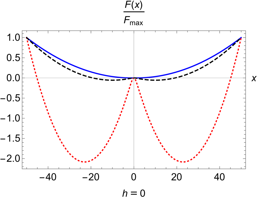
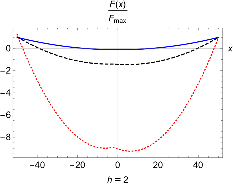
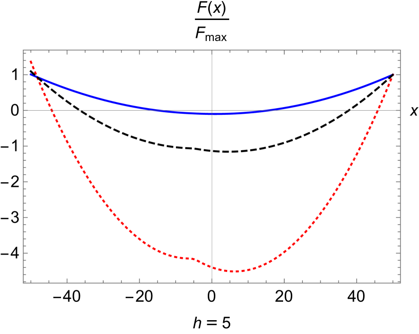
We focus on the limit of large , , when the integrals in (3.5) become concentrated in the small vicinity of the minimum [or two minima, when has a double-well form] of , defined by
| (3.9) |
Differentiating (3.6), we find the following transcendental equation, which defines implicitly,
| (3.10) |
Further on, performing the integrals in (3.5) we find that and obey
| (3.11) |
Lastly, comparing (3.10) with and defined in (3.11) and the definition of the order parameter in (2.7), we conclude that has quite a lucid physical meaning: indeed, and hence, defines the outcome of the vote multiplied by .
3.2 The case B
The derivation of transcendental equations, which implicitly define the order parameters and is only slightly more involved. Since it follows essentially the same line of thought, we present these equations here without a derivation. We have that in the case B:
| (3.12) |
where
| (3.13) |
The expressions in (3.12) reduce to the ones in (3.11) for . Below we will discuss the behavior of the order parameters in the cases A and B for the distribution in (2.1).
4 Results for the distribution in (2.1). Case A
In the particular case when the distribution is given by (2.1), in the right-hand-side of (3.8) can be calculated exactly. In the leading in the limit order, we have
| (4.1) |
so that (3.10) becomes
| (4.2) |
Two latter coupled transcendental equations, together with (3.11), implicitly define the order parameters in the case A.
These equations, which have multivalued solutions for sufficiently large values of , are quite difficult to study analytically in the whole parameter range (numerical solution is possible, of course). Nonetheless, they permit us to get some general understanding of the behavior of the order parameters in the limiting cases of small and large . We consider first the limit , which corresponds to the limit of a linear response of a system to an external bias. In this limit, for sufficiently small , we have that in the leading in order the order parameter obeys
| (4.3) |
Since the prefactor in this dependence is positive definite for sufficiently small and , the order parameter is an increasing function of for small . Further on, we find that in this limit, the order parameter of the soft and of the spins obey
| (4.4) |
We notice that for sufficiently small , the order parameter is a decreasing function of , while increases with an increase of .
Within the opposite limit , we find from (4.2) that in the leading in order
| (4.5) |
implying that as . This means, in turn, that is a non-monotonous function of and that for a strong (excessive) bias, the outcome of the vote is always against the preferential candidate.
Regarding the behavior of two other order parameters, we notice that since is always positive definite (for ), the order parameter of the rigid spins as , which means that the whole subgroup of ordinary voters is in favor of the preferential candidate. On the contrary, the order parameter of the contrarians behaves, in the leading in order, as
| (4.6) |
i.e., is negative and is growing indefinitely by an absolute value with so that the order parameter for sufficiently small is always a monotonously decreasing function of . In conclusion, we have that in the case A, an excessive bias breaks the ties within the community, letting the ordinary voters to have an opinion in favor of the preferential candidate, and the contrarians to have an opinion against this candidate. However, overall at large , the contrarians dominate by increasing the strength of their opinion.
We proceed with the numerical analysis, which permits us to have a broader look at the behavior of such a mixture of mutually-interacting rigid and soft spins. In particular, it permits us to determine the order parameters at arbitrary, not necessarily small or big values of , to consider the situations with arbitrary values of the coupling and also to analyse the effect of the initial configuration. In our numerical Monte Carlo simulations, we first fix an initial configuration of the spin variables, (e.g., stipulating that initially all spins are pointing downwards, or upwards, or are in some mixed configuration), fix and , and then let the system equilibrate via standard Metropolis algorithm for a sufficiently long time (typically, for time steps) until it reaches an equilibrium configuration, which may, in general, be different from the initial one. The purpose of doing so is as follows: for sufficiently large and for , the ferromagnetic system under study acquires a spontaneous ‘‘magnetization’’ so that the order parameters and are no longer equal to zero, unlike the case of small when both . The order parameter , for example, attains two values , where positive and negative values are chosen by the system with equal probability. In other words, for , it is equally probable that the whole system will have a negative or a positive magnetization. By choosing the initial state, i.e., by forcing the spins to point in some direction, we break the symmetry between the negative and positive value ‘‘helping’’ the system to arrive into the state with a prescribed sign of magnetization.
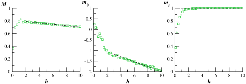
In figures 2, we first depict the order parameters as functions of for a small value of , and for an initial configuration in which all the spins are pointing upwards and which is let to equilibrate at a fixed and for time steps. We observe that for such a value of , upon an increase of , the order parameter of the rigid spins grows monotonously with and quite rapidly, already for , attains the limiting value . The order parameter of the soft spins, on the contrary, is a monotonously decreasing function of . This property also quite rapidly, already for , converges to the asymptotic form in (4.6). The combined effect of and is such that the order parameter first increases, being dominated by the rigid spins, passes through a maximal value, attained at , and then gradually decreases with , becoming dominated by the soft spins. Overall, we observe a very good agreement between the numerical results and our predictions for the asymptotic large- behavior.
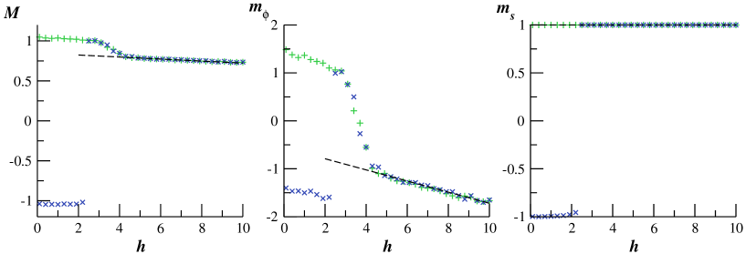
In figures 3 we plot the order parameters as functions of for a sufficiently big value of , , (such that the system may acquire a spontaneous magnetization at ), and also for two different initial configurations of spins. We start our discussion with the case when the initial configuration is most favorable for the preferential candidate — when all the rigid and the soft spins point upwards (curves depicted by pluses in figures 3) and then are let to equilibrate within time steps. In this situation, the order parameter of the rigid spins does not show any appreciable variation with and stays constant and equal to for any . The order parameter appears to be a monotonously decreasing function of and quite rapidly, already at , starts to converge to the asymptotic form in (4.6). Overall, the order parameter is also a monotonously decreasing function of , which means that prompting such a community to vote for a preferential candidate appears to be counter-productive even at very small values of .
For the initial configuration when all the spins — the rigid and the soft ones — point downwards and are let to equilibrate afterwards, the behavior of the order parameters appears to be more interesting and rich, and exhibits a seemingly discontinuous variation with the value of the external bias resembling true phase transitions in physical systems. We observe that here the order parameter stays equal to its value at , , up to a certain threshold value of , (which only slightly exceeds ), and then rather abruptly jumps to , when the bias becomes strong enough to pay the penalty set by the interaction energy with the soft spins. The order parameter first slightly decreases with an increase of and then abruptly jumps upwards, being turned over by the interactions with the rigid spins. In a way, one may claim that here the opinion of the contrarians gets inverted by the opinion of the ordinary voters. Further, monotonously decreases from the peak value and ultimately, for , converges to the asymptotic form in (4.6). The global order parameter , which represents the combined effect of the rigid and the soft spins, follows mostly the behavior of the order parameter of the soft spins and exhibits a discontinuous jump from to at , and then gradually decreases upon an increase of the external bias. Here, as well, we observe a very good agreement between the numerical data and our predictions for the asymptotic large- behavior.
5 Results for the distribution in (2.1). Case B
In this case, we have that the order parameter obeys a transcendental (3.12), which couples it to the order parameter . For the latter, performing the integrals in (3.13) with the distribution in (2.1), we find the following equation
| (5.1) |
As in the previous section, we start here with the solution of the coupled transcendental equations (3.12) and (5.1) in the limits and . In the limit of a linear response, we have
| (5.2) |
| (5.3) |
and
| (5.4) |
These expressions simplify to the ones given by (4.3) and (4.4) in which we set and, in principle, show a very similar behavior. On the contrary, the behavior in the limit appears to be quite different. At the same time, the order parameters and have the same linear dependence on [compare with (4.5) and (4.6)]; that being
| (5.5) |
and hence, both tend to when , the order parameter exhibits some novel and interesting features. The point is that, unlike the case A, here the argument in the hyperbolic tangent in (3.12) can be positive or negative depending on the value of the coupling parameter . More specifically, we have that for , where
| (5.6) |
the order parameter as , while for the order parameter . This means that in the case B, these are the soft spins which may turn over the rigid ones, present in majority. This is an opposite effect, as compared to the phenomenon which we observed for the case A.
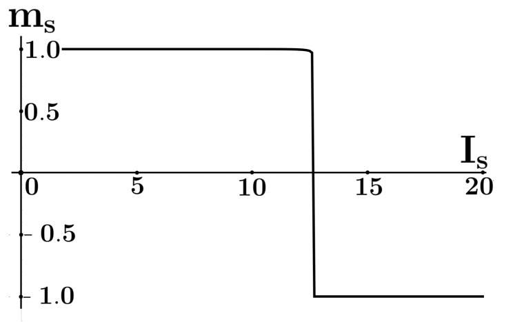
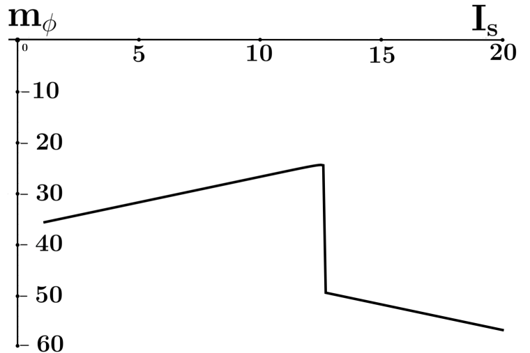
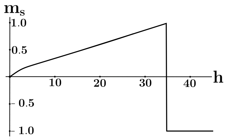
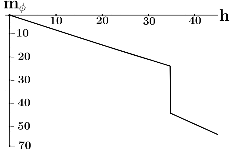
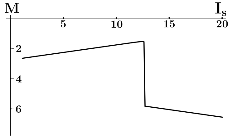
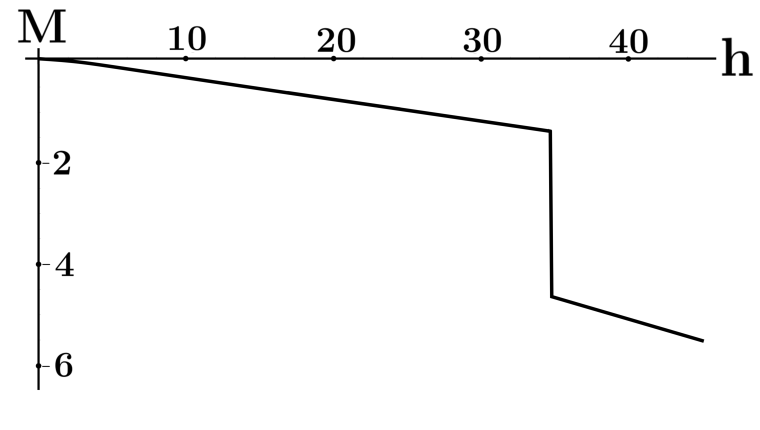
We illustrate the inversion of the rigid spins by the soft ones by solving the coupled transcendental equations (3.12) and (5.1) numerically, which also permits us to highlight some interesting features of the behavior at the intermediate values of and . In figures 4 we depict and as functions of for fixed and . We observe that is a growing function of for . At , the order parameter abruptly jumps downwards and starts to decrease with a further increase of . The downward jump of provokes all the rigid spins to turn over their direction, so that discontinuously changes from to . Further, in figures 5 we plot and as functions of for fixed and . We notice that is a decreasing function of with a discontinuous downward jump at . The order parameter first is an increasing function of , up to the value of at which jumps down: here, as well, exhibits a discontinuous jump to and stays constant further. Lastly, in figure 6, we depict the global order parameter as a function of (left-hand panel) and as a function of (right-hand panel). We observe that its behavior is entirely dominated by the behavior of the order parameter of the soft spins.
Conclusions
To recap, we have studied here a toy model of opinion formation in a mixed society consisting of two groups of individuals, interacting all with all across both groups, and that differ in their response to an external bias favoring one of two potential candidates in elections. While one group of individuals, present in majority, is characterized by their eagerness to accept the externally favored candidate, the minority group — the contrarians — are antagonistic to the bias and tend to have an opinion different from the externally imposed one. Modelling such a society as a system of appropriately defined interacting, effective spin variables, we arrive at a general conclusion that pushing too strongly for the preferential candidate appears to be counter-productive and leads to a smaller effect than the one achieved with a modest bias. We show, as well, that depending on how the interactions between the two groups and within each of the groups are defined, interesting phenomena of an opinion turn-over can take place, when either of two groups can abruptly change its opinion in favor of the opinion of another group.
Acknowledgements
We express our warmest thanks to Dr. Olesya Mryglod for her interest in this work and stimulating communications. C.M.-M. acknowledges a partial support from the Spanish MICINN grant MTM2015-63914-P.
References
- [1] Conwell E., Phys. Today, 1970, 23, 35; doi:10.1063/1.3022161.
-
[2]
Nava F., Canali C., Catellani F., Gavioli G., Ottaviani G., J. Phys. C: Solid State Phys., 1976, 9, 1685;
doi:10.1088/0022-3719/9/9/010. - [3] Stanton C.J., Baranger H.U., Wilkins J.W., Appl. Phys. Lett., 1986, 49, 176; doi:10.1063/1.97216.
- [4] Lei X.L., Horing N.J.M., Cui H.L., Phys. Rev. Lett., 1991, 66, 3277; doi:10.1103/PhysRevLett.66.3277.
- [5] Böttger H., Bryksin V.V., Phys. Status Solidi B, 1982, 113, 9; doi:10.1002/pssb.2221130102.
- [6] Barma M., Dhar D., J. Phys. C: Solid State Phys., 1983, 16, 1451; doi:10.1088/0022-3719/16/8/014.
- [7] Vrhovac S.B., Petrović Z.Lj., Phys. Rev. E, 1996, 53, 4012; doi:10.1103/PhysRevE.53.4012.
- [8] Slater G.W., Guo H.L., Nixon G.I., Phys. Rev. Lett., 1997, 78, 1170; doi:10.1103/PhysRevLett.78.1170.
- [9] Kostur M., Machura L., Hänggi P., Łuczka J., Talkner P., Physica A, 2006, 371, 20; doi:10.1016/j.physa.2006.04.086.
- [10] Oshanin G., Klafter J., Urbakh M., Europhys. Lett., 2004, 68, 26; doi:10.1209/epl/i2003-10311-0.
- [11] Oshanin G., Klafter J., Urbakh M., J. Phys.: Condens. Matter, 2005, 17, S3697; doi:10.1088/0953-8984/17/47/004.
- [12] Jack R.L., Kelsey D., Garrahan J.P., Chandler D., Phys. Rev. E, 2008, 78, 011506; doi:10.1103/PhysRevE.78.011506.
- [13] Baiesi M., Maes C., Wynants B., Phys. Rev. Lett., 2009, 103, 010602; doi:10.1103/PhysRevLett.103.010602.
- [14] Leitmann S., Franosch T., Phys. Rev. Lett., 2013, 111, 190603; doi:10.1103/PhysRevLett.111.190603.
- [15] Baerts P., Basu U., Maes C., Safaverdi S., Phys. Rev. E, 2013, 88, 052109; doi:10.1103/PhysRevE.88.052109.
- [16] Baiesi M., Maes C., New J. Phys., 2013, 15, 013004; doi:10.1088/1367-2630/15/1/013004.
-
[17]
Bénichou O., Illien P., Oshanin G., Sarracino A., Voituriez R., Phys. Rev. Lett., 2014, 113, 268002;
doi:10.1103/PhysRevLett.113.268002. - [18] Baiesi M., Falasco G., Phys. Rev. E, 2015, 92, 042162; doi:10.1103/PhysRevE.92.042162.
-
[19]
Bénichou O., Illien P., Oshanin G., Sarracino A., Voituriez R., Phys. Rev. E, 2016, 93, 032128;
doi:10.1103/PhysRevE.93.032128. - [20] Cividini J., Mukamel D., Posch H.A., Phys. Rev. E, 2017, 95, 012110; doi:10.1103/PhysRevE.95.012110.
-
[21]
Sarracino A., Cecconi F., Puglisi A., Vulpiani A., Phys. Rev. Lett., 2016, 117, 174501;
doi:10.1103/PhysRevLett.117.174501. -
[22]
Bénichou O., Illien P., Mejía-Monasterio C., Oshanin G., J. Stat. Mech.: Theory Exp., 2013, 2013, P05008;
doi:10.1088/1742-5468/2013/05/P05008. - [23] Bénichou O., Bodrova A., Chakraborty D., Illien P., Law A., Mejía-Monasterio C., Oshanin G., Voituriez R., Phys. Rev. Lett., 2013, 111, 260601; doi:10.1103/PhysRevLett.111.260601.
-
[24]
Illien P., Bénichou O., Oshanin G., Voituriez R., Phys. Rev. Lett., 2014, 113, 030603;
doi:10.1103/PhysRevLett.113.030603. - [25] Leitmann S., Franosch T., Phys. Rev. Lett., 2017, 118, 018001; doi:10.1103/PhysRevLett.118.018001.
- [26] Benenti G., Casati G., Prosen T., Rossini D., EPL, 2009, 85, 37001; doi:10.1209/0295-5075/85/37001.
- [27] Wald S., Henkel M., J. Phys. A: Math. Theor., 2016, 49, 125001; doi:10.1088/1751-8113/49/12/125001.
- [28] Zia R.K.P., Praestgaard E.L., Mouritsen O.G., Am. J. Phys., 2002, 70, 384; doi:10.1119/1.1427088.
- [29] Galam S., Physica A, 2004, 333, 453; doi:10.1016/j.physa.2003.10.041.
- [30] Sen P., Chakrabarty B.K., Sociophysics: an Introduction, Oxford University Press, New York, 2014.
Ukrainian \adddialect\l@ukrainian0 \l@ukrainian
Негативний вiдгук на надлишкове вiдхилення, спричинене змiшаною популяцiєю виборцiв []В.С. Доценко, К. Мехiя-Монастерiо, Г. Ошанiн
Лабораторiя теоретичної фiзики конденсованої матерiї, UPMC,
CNRS UMR 7600, унiверситет Сорбонна, 75252 Париж, Францiя
Лабораторiя фiзичних властивостей, Мадридський технiчний унiверситет, 28040 Мадрид, Iспанiя