Mobility tensor of a sphere moving on a super-hydrophobic wall: application to particle separation

Abstract

The paper addresses the hydrodynamic behavior of a sphere close to a micro-patterned superhydrophobic surface described in terms of alternated no-slip and perfect-slip stripes. Physically, the perfect-slip stripes model the parallel grooves where a large gas cushion forms between fluid and solid wall, giving rise to slippage at the gas-liquid interface. The potential of the boundary element method (BEM) in dealing with mixed no-slip/perfect-slip boundary conditions is exploited to systematically calculate the mobility tensor for different particle-to-wall relative positions and for different particle radii. The particle hydrodynamics is characterized by a non trivial mobility field which presents a distinct near wall behavior where the wall patterning directly affects the particle motion. In the far field, the effects of the wall pattern can be accurately represented via an effective description in terms of a homogeneous wall with a suitably defined apparent slippage. The trajectory of the sphere under the action of an external force is also described in some detail. A “resonant” regime is found when the frequency of the transversal component of the force matches a characteristic crossing frequency imposed by the wall pattern. It is found that, under resonance, the particle undergoes a mean transversal drift. Since the resonance condition depends on the particle radius the effect can in principle be used to conceive devices for particle sorting based on superhydrophobic surfaces.

1 Introduction

Super-hydrophobic (SH) surfaces have raised a large interest in the last decades for their self-cleaning [1, 2] and drag reducing [3, 4, 5, 6] properties. These features are associated with gas or vapor bubbles trapped into the asperities of the solid surface. Commonly SH surfaces are fabricated by patterning the solid substrate with regular micro-structures (holes, grooves, pillars). In presence of a hydrophobic substrate, the liquid, usually water, hardly penetrates the hollows. This state is called the Cassie-Baxter state (also known as fakir-state). In the Cassie-Baxter state the liquid is in contact with a patterned boundary consisting of alternated regions of liquid-solid and liquid-air/vapor interfaces.

Since the trapped air or vapor acts as an almost perfect-slip cushion a simple model of a SH surface is given as a smooth wall with patterned boundary conditions. The standard no-slip condition applies to the liquid-solid interface and the perfect-slip condition at the liquid-air/vapor interface [4, 7].

Purpose of the present paper is analyzing the hydrodynamics of a micrometer bead moving close to a SH surface. The patterned wall is modeled with alternating perfect-slip/no-slip parallel stripes (Fig. 1). All the typical length scales (particle radius, wall pattern length, and particle-wall gap) considered here are on the order of micrometers, sufficiently large to describe the fluid as a continuum obeying the Navier-Stokes equations [8, 9, 10, 11, 12] with no slippage at the solid wall [13, 14, 15, 16, 17, 18, 19]. Our model corresponds to the real case of sufficiently deep grooves where it can be safely assumed perfect-slip at the liquid-gas interface, see e.g. the discussion reported in [20, 21]. At the same time the particle is sufficiently small to neglect fluid inertia in the limit of vanishing Reynolds number. Following standard dimensional analysis, the fluid acceleration in the Navier Stokes equations can be neglected altogether leading to the linearized time independent Stokes equations [22]. In these conditions, the coupling between the particle and the fluid is entirely described by the mobility tensor field ${\vec{M}}({\vec{x}})$. In fact, for any particle position $\vec{x}$ the solution of the Stokes problem is achieved by using the so-called Boundary Element Method (BEM) where the system of partial differential equations is rewritten in terms of a vector boundary integral equation. The unknown reduces to the complementary data at the boundary, the stress vector where velocity (no-slip) is enforced or the velocity where the stress is prescribed (perfect-slip). From the Stokes solution the mobility tensor can be calculated, see e.g. [23] for details. The $\vec{x}$ dependence of the mobility field is then recovered by placing the particle at different positions with respect to the patterned wall. The mobility tensor summarizes all the relevant hydrodynamic information needed to solve for the particle trajectory, once external forces are applied. All the complexity due to the patterned wall is lumped together in the mobility tensor field allowing for a simple parametric study of the particle response.

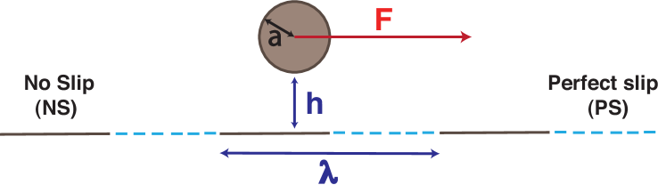
Figure 1: System geometry. A sphere of radius $a$ moves at a distance $h$ from a planar wall. The wall is a superhydrophobic surface in Cassie state with a flat meniscus. The pattern period is indicated with $\lambda$. The perfect-slip condition is used at the air/liquid interface (PS, dashed line) and the no-slip condition is used at the solid-liquid interface (NS, solid line).

2 Mathematical model

The linear Stokes system,

$$\nabla\cdot\vec{u}=0$$ (1)

$$\nabla^{2}{\vec{u}}-\vec{\nabla}{p}=0 \;,$$ (2)

for the velocity ${\bf u}$ and the pressure $p$, here written in dimensionless form with half the perfect-slip stripe width $w$ as reference length and $\mu/(w\rho)$ and $\mu^{2}/(\rho w^{2})$ as velocity and pressure scale respectively, is recast in terms of a boundary integral formulation

$$E(\mbox{\boldmath$\xi$})u_{j}(\mbox{\boldmath$\xi$}) = \frac{1}{8\pi}\oint_{\partial\Omega}t_{i}({\bf x})G_{ij}({\bf x},\mbox{\boldmath$\xi$})\,dS_{{\bf x}}-$$ (3)

$$\frac{1}{8\pi}\oint_{\partial\Omega}u_{i}({\bf x}){\cal T}_{ijk}({\bf x},\mbox{\boldmath$\xi$})n_{k}({\bf x})\,dS_{{\bf x}}.$$

Here $\partial\Omega$ is the boundary of the flow domain $\Omega$, which consists of the particle surface and the patterned wall. $G_{ij}$ is the fundamental solution (free-space Green’s function or Stokeslet), ${\cal T}_{ijk}$ the associated stress tensor, $u_{i}$ the i-th velocity component and $t_{i}$ the traction vector, $t_{i}=-p\delta_{ij}+\partial u_{i}/\partial x_{j}+\partial u_{j}/\partial x_{i}$ with $\delta_{ij}$ the Kronecker delta. The velocity at $\xi$ is expressed as the convolution of the densities (velocity and stress vector) with the appropriate convolution kernels (Green’s function tensor and associated stress). The coefficient $E$ equals $1$ inside the fluid domain and $1/2$ at regular boundary points, respectively. Collocating the representation at boundary points provides a boundary integral equation where the unknowns are the complementary data to those prescribed at the boundaries (i.e. the unknown is the velocity where the traction vector is prescribed and the traction vector where the velocity is given). In the present case the data are the velocity where no-slip holds and a combination of vanishing wall-normal velocity and tangential traction at the impermeable perfect slip regions. The integral equation can be solved numerically by the so-called boundary element method [24, 23], a standard approach for linear systems of partial differential equation with constant coefficients (see the Appendix for a few more details). After the traction at the particle surface is evaluated, the hydrodynamic forces and torques are obtained by integration thus determining the resistance matrix and, by inversion, the mobility tensor.

In all the cases considered below, the solid fraction $0\leq\phi_{s}\leq 1$ of the patterned wall, ratio of no-slip to total surface area, is $\phi_{s}=0.5$ (equal width for the perfect-slip and the no-slip stripes), such that the dimensionless pattern periodicity is $\lambda=4$ (see sketch in Fig. 1). No difficulty is found to extend the numerical model to other solid fractions, provide resolution issues are treated with adequate care for the extreme cases (very small or very large $\phi_{s}$). In the following, unless otherwise explicitly stated, only the case of a no-slip particle will be addressed. Again, given the flexibility of the approach, no substantial difficulty is encountered for different boundary conditions (perfect-slip or partial slip boundary conditions at the particle boundary). The SH wall coincides with the $Oxy$ plane of the reference system with the alternating perfect-slip (PS) and no-slip (NS) stripes parallel to the $y$ axis (see Fig. 1) being $z$ the wall-normal coordinate. Where convenient, the different components of vectors and tensors will be denoted by indices, e.g. $x\equiv x_{1}$, $y\equiv x_{2}$, and $z\equiv x_{3}$. The dimensionless sphere radius is $a$ with $h$ the normalized gap between sphere and wall.

In the context of Stokes flows, the response is linear with respect to the external force applied to the particle. It follows that the problem of determining the linear and angular velocity of the sphere, given forces and torques, can be conveniently formulated in terms of the mobility tensor $M_{\alpha\,\beta}$, $\alpha,\,\beta=1,\ldots 6$, see e.g. the classical textbook [23]. Indeed the mobility tensor relates the generalized (linear and angular) velocities to the generalized forces (forces and torques), namely

$$\left[\begin{array}[]{c}U_{1}\\ U_{2}\\ U_{3}\\ \omega_{1}\\ \omega_{2}\\ \omega_{3}\\ \end{array}\right]=\left[\begin{array}[]{cccccc}M_{11}&M_{12}&M_{13}&M_{14}&M_{15}&M_{16}\\ M_{21}&M_{22}&M_{23}&M_{24}&M_{25}&M_{26}\\ M_{31}&M_{32}&M_{33}&M_{34}&M_{35}&M_{36}\\ M_{41}&M_{42}&M_{43}&M_{44}&M_{45}&M_{46}\\ M_{51}&M_{52}&M_{53}&M_{54}&M_{55}&M_{56}\\ M_{61}&M_{62}&M_{63}&M_{64}&M_{65}&M_{66}\end{array}\right]\left[\begin{array}[]{c}F_{1}\\ F_{2}\\ F_{3}\\ T_{1}\\ T_{2}\\ T_{3}\\ \end{array}\right]$$ (4)

where $U_{i}$, $i=1,\ldots 3$, are the components of the particle center velocity $\vec{U}$, $\omega_{i}$ the components of the angular velocity $\omega$, and $F_{i}$ and $T_{i}$ are the components of force $\vec{F}$ and torque $\vec{T}$, respectively. With this notation $M_{i,\,j+3}$ gives the coupling between the j-th component of the torque and i-th component of the linear velocity of the sphere. The reciprocity theorem guarantees the symmetry of the mobility tensor, $M_{\alpha\beta}=M_{\beta\alpha}$. In more compact notation eq. (4) is rewritten as

$$\vec{\tilde{U}}=\vec{M}\cdot\vec{\tilde{F}}$$ (5)

where $\vec{\tilde{U}}$ and $\vec{\tilde{F}}$ are the generalized velocities and forces and $\vec{M}$ is the mobility tensor. In the general case the mobility is a tensor field $\vec{M}(\vec{x})$ depending on the position of the sphere center. The symmetry of the problem induces a corresponding symmetry on the tensor field. For instance, in free space the mobility tensor reduces to a diagonal matrix for a spherical body, consistently with the absence of any coupling among the different degrees of freedom. A homogeneous wall breaks the translation symmetry of the sphere in the wall-normal direction and induces the coupling between wall-parallel translations in direction ${\vec{\hat{e}}}$ and wall parallel rotations with axis parallel to ${\vec{\hat{z}}}\times{\vec{\hat{e}}}$ where ${\vec{\hat{e}}}$ is any wall parallel unit vector and ${\vec{\hat{z}}}$ is the wall-normal unit vector pointing towards the fluid, respectively, see e.g. the review [25] and the textbook [23].

3 Sphere moving along a homogeneous wall

The solution of the Stokes equations (2) in the geometry described in Fig. 1 is obtained by an in-house boundary element code based on the BEMLIB library released by Pozrikidis [26]. This approach allows to tackle complex boundaries where the complexity relies both on the geometrical configuration and on the assigned boundary conditions, the alternation of PS/NS regions in the present case, Appendix A. When dealing with wall bounded Stokes flows, the effect of a single planar wall can in principle be included in the Green’s function (wall Green function) thus avoiding the discretization of the wall itself, see e.g. [27]. However the use of a specialized Green’s function becomes too cumbersome to deal with alternated PS/NS boundary conditions at the wall as required to model the present SH surface. It is more convenient to work with the free-space Green’s function and use a boundary integral equation extending to particle and wall surfaces. Clearly, the infinite planar wall is truncated in numerics where it is modeled as a finite square of size $L\gg\lambda$. The appropriate truncation length $L$, in the range of sphere-to-wall clearance $h$ considered here, is selected by comparison with the results of the wall Green function formulation (corresponding to an actually infinite wall) for the simple case of a no-slip wall.

3.1 No-slip wall

A first validation of the numerics concerns the sphere in free space. As for the homogeneous wall, the reference length $w$ introduced in the previous section is, strictly speaking, undefined. It is fixed in this case by requiring the dimensionless sphere radius to be $a=1$. The numerically estimated resistance of the no-slip sphere in free space was checked to recover the well known Stokes results for rigid body translation in direction ${\vec{\hat{e}}}$ and rigid body rotation ${\vec{\omega}}$, ${\vec{D}}=-6\pi a{\vec{\hat{e}}}$ and ${\vec{Q}}=-8\pi a{\vec{\omega}}$, respectively. It may be worthwhile calling the reader’s attention on the fact that ${\vec{F}}$ and ${\vec{T}}$ as defined in eq. (4) are external forces applied to the sphere while ${\vec{D}}$ and ${\vec{Q}}$ denote the drag force and torque experienced by the sphere in the relative motion with respect to the fluid. In other words, for constant translation and rotation velocities, ${\vec{D}}+{\vec{F}}=0$ and ${\vec{Q}}+{\vec{T}}=0$. As a second check the drag law for the perfect-slip sphere moving in direction ${\vec{\hat{e}}}$, ${\vec{D}}=-4\pi a{\vec{\hat{e}}}$ and ${\vec{Q}}=0$, was also reproduced, see [28].

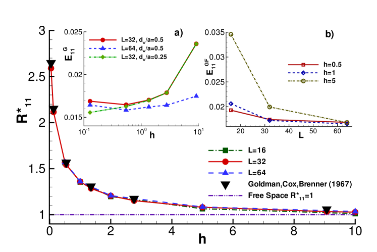
Figure 2: Main panel: The $R_{11}^{*}$ resistance coefficient of a sphere of radius $a=1$ over a truncated no-slip wall plotted against the gap $h$ for three different truncation lengths: $L=16$ (squares, dash-dotted line), $L=32$ (circles, solid line), $L=64$ (triangles, dashed line). Black inverted triangles refer to the analytical solution by Goldman, Cox and Brenner [29]. Inset $a)$: relative error between the present data and [29], $E^{G}_{11}=(R^{G}_{11}-R_{11})/R^{G}_{11}$ where the superscript $G$ refers to Goldman et al., for $L=32$ and $L=64$. Inset b): relative error $E^{GF}_{11}=(R^{GF}_{11}-R_{11})/R^{GF}_{11}$, where $GF$ refers to numerical results obtained by using the Green Function for an infinite no-slip wall [27], plotted against $L$ for three different gaps: $h=0.5$ (squares, solid line), $h=1$ (diamonds, dashed line), $h=5$ (circles, dash-dotted line).

More interesting are the tests in presence of the wall. In Stokes flows the velocity disturbance decays in space as the inverse distance from the momentum source, i.e. the sphere in the present case, as easily shown from the far field asymptotic of representation (3) where $G_{ij}\sim 1/r$. For this reason domain truncation effects must be carefully addressed. In presence of a homogeneous wall, the hydrodynamic force ${\vec{D}}$ due to a wall-parallel translation of the sphere in direction ${\vec{\hat{e}}}$ has, by symmetry, a vanishing wall normal component $D_{3}$. Indeed, $D_{3}$ depends linearly on the particle velocity and should change sign under velocity inversion. Clearly $D_{3}$ should instead be independent of the direction of the wall parallel velocity. The only possible conclusion is that $D_{3}\equiv 0$. Hence the only non vanishing component of the hydrodynamic force is the one opposed to the velocity,

$$R_{11}=R_{22}=-{\vec{D}}\cdot{\vec{\hat{e}}}={\vec{\hat{e}}}\cdot\int_{\partial B}{\vec{t}}dS>0\,,$$

where $\vec{t}$ is the stress exerted by the body on the fluid. Figure 2 shows the normalized resistance coefficient $R_{11}^{*}=R_{11}/(6\pi a)$ for a no-slip sphere of radius $a=1$ moving in the wall parallel direction ${\vec{\hat{e}}}_{1}$ close to a no-slip wall. Data are reported as a function of the gap $h$ for different domain truncation lengths $L$. As $L$ is increased the results show apparent convergence toward the infinite wall result, compare data at $L=32$ and $L=64$. For further comparison the analytic results obtained in [29] are also reported. The resistance coefficient $R^{GF}_{11}$ for the actual infinite planar wall was also obtained by using a companion numerical solution that employed the wall Green function. The inset a) concerns the relative error, $E^{G}_{11}=(R^{G}_{11}-R_{11})/R^{G}_{11}$ where the superscript $G$ refers to Goldman et al., between the present numerics and the analytical solution of [29]. The three curves correspond to a reference solution with $L=32$ and a characteristic wall panel dimension $d_{w}/a=0.5$, to a second solution with the same truncation length and a finer discretization $d_{w}/a=0.25$, and to a third case with the same grid of the reference numerical solution and increased truncation length $L=64$. From the comparison it is apparent that the typical panel dimension controls the error when the particle is close to the wall. Instead, when the wall-normal distance increases the effect of truncation becomes dominant, requiring a larger portion of the wall to be retained in the numerical configuration. The inset b) reports the relative error $E^{GF}_{11}=(R_{11}-R^{GF}_{11})/R^{GF}_{11}$ with respect to the wall-Green Function approach vs the truncation length $L$ for different gaps $h$. As already commented on, $E^{GF}_{11}$ increases with $h$ at fixed wall truncation and decreases with $L$ at fixed wall distance, confirming that a finite portion of the planar wall is seen to better approximate the infinite wall case when the distance of the object from the wall gets smaller and smaller. For the typical gaps to be further considered in this paper, namely $h\in(0.125,2)$, no significant improvements are achieved by increasing $L$ from $32$ to $64$ with the relative error in both cases below $\sim 2\%$. Hence, where not explicitly stated, the value $L=32$ is used throughout the paper. Similar convergence is observed for all other non-zero resistance tensor coefficients (data not shown). For this range of parameters the particle surface was discretized by means of a hierarchical triangular mesh of $512$ elements whose typical size is $d_{p}/a=0.1567$. A non-uniform discretization consisting of about $1500$ elements is adopted for the wall. In fact, the tessellation of the wall is locally refined below the sphere and is progressively coarsened away from it.

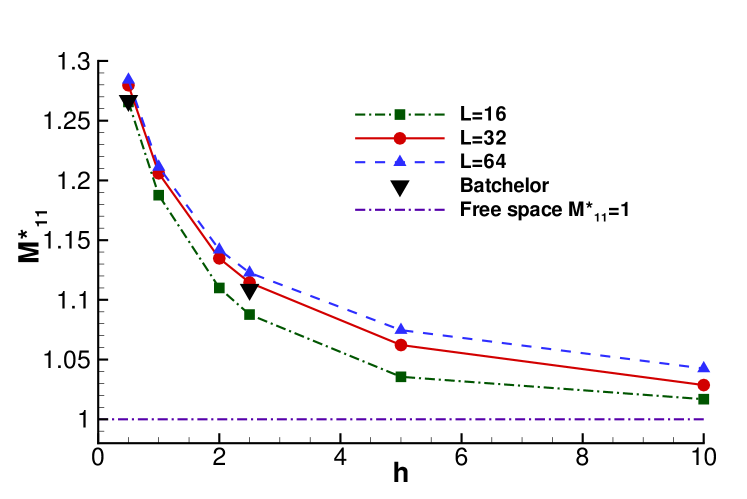
Figure 3: Mobility coefficient $M_{11}^{*}$ of a no-slip solid sphere of radius $a=1$ in presence of a perfect-slip wall as a function of the sphere-to-wall gap $h$ for different wall truncations $L=16$ (squares, dashed line), $L=32$ (circles, dash-dotted line), $L=64$ (triangles, solid line). Black inverted triangles refer to the analytical solution by Batchelor [30].

3.2 Perfect-slip wall

After the preliminary validation provided in the previous subsection, numerical results worth being discussed concern the motion of a no-slip sphere close to a perfect-slip homogeneous wall. In this case symmetry considerations can be exploited to provide a reference solution to compare the present result with. Indeed considering the image of the sphere with respect to the perfect slip wall one ends up with a two-sphere system translating parallel to the wall in otherwise infinite space. By symmetry it is clear that taking the two-sphere solution restricted to the half-space above the wall provides the required solution for the present perfect-slip wall problem. The solution of two-sphere problem was discussed by Batchelor [30] where reference data for the mobility are provided. Alternatively, one can exploit the equivalent two sphere problem to derive a boundary integral equation only involving the unknown traction on the physical sphere that accounts for its image below the wall in such a way that the solution provides the desired results for the perfect slip wall case.

The main results are summarized in Fig. 3 where the mobility coefficient $M_{11}^{*}$ for the sphere is reported as a function of the dimensionless gap $h$. Even in this case a few wall truncation lengths are considered, namely $L=16,\,32,\,64$. As expected $M_{11}^{*}$ decreases (resistance increases) approaching the free-space value for increasing gap. On the contrary the mobility coefficient increases (resistance lowers) when the gap is progressively reduced. This is a consequence of the perfect-slip boundary condition that allows a finite fluid velocity at the wall. It follows that strong velocity gradients can not occur in the gap between sphere and wall in contrast to the case of a no-slip surface. Also in this case the numerical solution shows good agreement with respect to the equivalent Batchelor two-sphere problem (black inverted triangles in Fig. 3). Even for the perfect-slip wall the results are only negligibly affected by the wall truncation for sufficiently large $L$ , as shown by comparing $M_{11}^{*}$ at $L=32$ and $L=64$ for the present values of the gap $h\in(0.125,2)$.

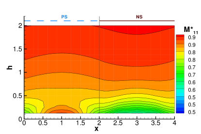
(a) a=0.25

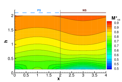
(b) a=0.5

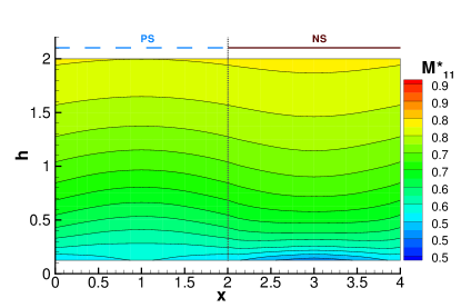
(c) a=1

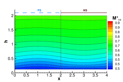
(d) a=2

Figure 4: $M^{*}_{11}$ fields for different sphere radii. Near the wall the mobility strongly depends on the $x-$ position of the sphere center. The $x-$dependence is weakened as the gap $h$ is increased.

4 Mobility tensor for a superhydrophobic wall

By symmetry, the matrix representing the mobility tensor of a sphere close to the superhydrophobic surface sketched in Fig.1, takes on a checkerboard structure. The (symmetric) matrix can easily be recast into block-diagonal form by a simple reordering of generalized velocity and forces, namely

$$\left[\begin{array}[]{c}U_{1}\\ \omega_{2}\\ U_{3}\\ \omega_{1}\\ U_{2}\\ \omega_{3}\\ \end{array}\right]=\left[\begin{array}[]{cccccc}M_{11}&M_{15}&M_{13}&0&0&0\\ M_{15}&M_{55}&M_{35}&0&0&0\\ M_{13}&M_{35}&M_{33}&0&0&0\\ 0&0&0&M_{44}&M_{24}&M_{46}\\ 0&0&0&M_{24}&M_{22}&M_{26}\\ 0&0&0&M_{46}&M_{26}&M_{66}\\ \end{array}\right]\left[\begin{array}[]{c}F_{1}\\ M_{2}\\ F_{3}\\ M_{1}\\ F_{2}\\ M_{3}\\ \end{array}\right].$$ (6)

In this form the cross-coupling between the different degrees of freedom becomes apparent showing, e.g., that the rotation around the axis parallel to the stripes ($x_{2}$) couples with a force in the wall-normal direction $x_{3}$ through the mobility coefficient $M_{53}=M_{35}$. The mobility tensor depends on the wall-normal distance expressed by the gap clearance $h$ and on the wall-parallel coordinate normal to the stripes $x_{1}=x$, $M_{\alpha\beta}(x,h)$.

In the following the (dimensionless) mobility tensor is normalized by the free stream value $M_{11}^{\infty}=1/(6\pi a)$, $\vec{M}^{*}=\vec{M}/M_{11}^{\infty}$. Figure 4 reports $M^{*}_{11}$ as a function of $h$ and $x$ for different particle radii $a=0.25,0.5,1,2$. Apparently $M^{*}_{11}$ is symmetric with respect to the center of both the perfect-slip ($x=1$) and the no slip ($x=3$) stripe. Two features of the plots are noteworthy. $i)$ Far from the wall $M^{*}_{11}$ is unexpectedly larger for $x\in(2,4)$ (i.e. when the center of the sphere is above the no-slip stripe) than for $x\in(0,2)$ (sphere above the perfect-slip stripe). $ii)$ This behavior is reversed close to the wall where, as expected, $M^{*}_{11}$ is larger above the perfect slip stripe, see cases $a=0.25$ and $a=0.5$ in particular.

In Fig. 5 $M^{*}_{11}$ is reported as a function of $h$ for different particle positions $x$ for $a=0.5$. Two distinct regions can be identified: a near-wall and a far field region. In the near wall region the mobility coefficient is larger for $x$ corresponding to the perfect slip stripe and strongly depends on the position along the wall pattern. In the far field the mobility is larger for $x$ corresponding to the no slip portion of the wall, with a less pronounced $x$-dependence and a monotonic approach to the free space value (recovered up to 90% at $h=2$). In order to define the two regions, their boundary is set at the gap $h_{inv}$ where $M^{*}_{11}(1,h_{inv})=M^{*}_{11}(3,h_{inv})$ (i.e. the gap where the mobility for a particle above the PS stripe equals the mobility above the NS stripe). From the inset of Fig. 5 it is apparent that $h_{inv}$ decreases with the particle radius.

Figure 6 shows the dimensionless averaged mobility coefficient $\langle M^{*}_{11}\rangle$ as a function of the gap-to-particle-radius ratio, $h/a$, for spheres of different radii. The angular brackets denotes the spatial average of the complete field $M^{*}_{11}(x,h)$ in the periodic direction $x$. In the plot the present data (symbols) are compared against the mobility over a homogeneous wall with a suitably defined partial slip boundary condition (solid lines),

$${u_{x/y}}|_{w}=\ell_{x/y}\frac{\partial u_{x/y}}{\partial z}\Big{|}_{w}\ .$$ (7)

Philip formula [7, 4] expresses the effective slip lengths, $\ell_{x}$ and $\ell_{y}$, in the longitudinal and transversal directions to the stripes, in terms of the pattern solid fraction $\phi_{s}$ and length $\lambda$,

$$\ell_{y}=2\ell_{x}=\frac{1}{\pi}\ln\left\{\sec\left[\frac{\pi\left(1-\phi_{s}\right)}{2}\right]\right\}\ .$$ (8)

In the original papers these expressions were derived for a flow over a patterned wall dragged by a constant shear stress in the far field. The same expressions are used here to reconstruct an effective wall boundary condition to model the fluid-wall interaction in the case of the moving sphere over the patterned surface. In other words eqs. (7,8) are used as boundary conditions at the patterned wall in the BEM solver. Figure 6 shows that, as $h/a$ is increased, the mobility approaches the free-space value independently of the detailed boundary condition used at the patterned wall. For further comparison also the data pertaining to a homogeneous no-slip wall are reported (dashed lines). The mobility profiles calculated with the partial-slip boundary condition closely follows those computed for the actually patterned wall for nearly all the considered gaps. Clearly the accuracy in reconstructing the correct mobility is better in the far field region, even though the discrepancy is always below 5% in the worst cases when the sphere gets closest to the wall. These results indicate that the spatially average mobility experienced by the particle is weakly dependent on the geometrical details of the wall pattern and can be described by a suitably defined effective slippage at the wall. The mobility profiles $M^{*}_{11}(x=1,h)$ extracted at the center of the perfect-slip region are plotted in the inset of Fig. 6.

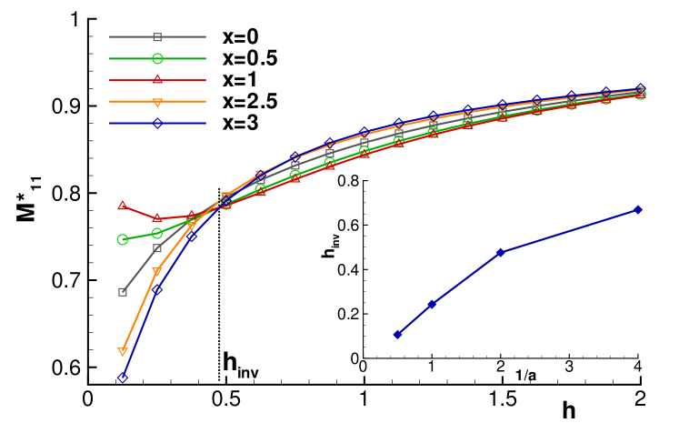
Figure 5: $M^{*}_{11}$ as a function of the gap $h$ for different $x$ ($a=0.5$). Different behaviors are observed in the near wall region $h<h_{inv}$ and in the far field $h>h_{inv}$. Near the wall strong changes occur when moving the particle from a perfect-slip stripe (e.g. $x=1$) to a no-slip stripe (e.g. $x=3$) and the mobility is larger above a perfect-slip than above a no-slip stripe. In the far field $M^{*}_{11}$ is more uniform in $x$ and the mobility of the particle is larger just above a no-slip stripe. In the inset, inversion gap $h_{inv}$ for different particle radii.

In the near wall region ($h<h_{inv}$) the mobility is strongly affected by the perfect-slip stripe and, at least for the spheres of radius $a=0.25,0.5$ (i.e. for a sphere diameter smaller than one stripe width), a mobility minimum is achieved at a certain (small) distance from the wall. The location of the minimum approaches the wall as the sphere radius is increased. In the far field ($h>h_{inv}$, dashed vertical lines), the mobility approaches the free-space value closely following the curves obtained from the effective slip model of the wall.

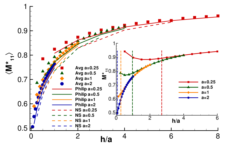
Figure 6: Mobility profiles as a function of $h/a$ for particles of different radii $a\in[0.25;2]$. Spatially averaged mobility $\langle M^{*}_{11}\rangle$ for the patterned wall (symbols). Mobility of an homogeneous wall with a partial slip boundary condition (solid lines). Non-slip homogeneous wall (dashed lines). Inset: $M^{*}_{11}$ profiles at the center of PS zone ($x=1$). The dashed vertical lines denote the critical distance $h_{inv}$.

The discussion of the mobility is completed in Fig. 7 which provides coefficients $M^{*}_{22}$ and $M^{*}_{13}$ for $a=0.5$. As expected $M^{*}_{13}$ is anti-symmetric with respect to the mid-point of the two stripes. For comparison, in free space the mobility matrix is purely diagonal and isotropic meaning that there is no coupling among the degrees of freedom, $M_{11}=M_{22}=M_{33}$, and $M_{44}=M_{55}=M_{66}$. A homogeneous wall in the $x-y$ plane breaks the homogeneity in the $z$-direction, i.e. $\vec{M}=\vec{M}(h)$ and introduces the coupling between translations in wall parallel directions and rotations along the orthogonal wall-parallel axis, see the discussion at the end of § 2. The coupling is provided by the mobility coefficients $M_{15}(h)=M_{24}(h)=M_{51}(h)=M_{42}(h)$. For the homogeneous wall the non vanishing terms are $M_{33}(h)$, $M_{11}(h)=M_{22}(h)$, $M_{15}(h)=M_{24}(h)=M_{51}(h)=M_{42}(h)$, $M_{66}(h)$, and $M_{44}(h)=M_{55}(h)$.

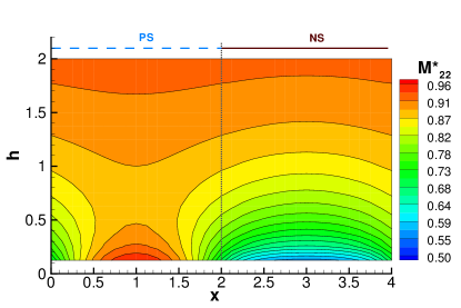
(a) $M^{*}_{22}$ field (a=0.5)

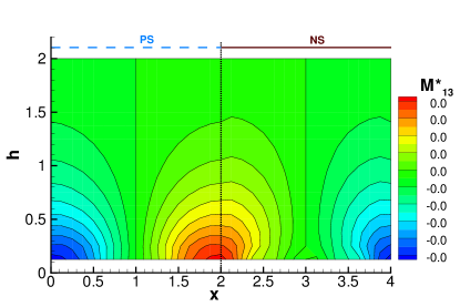
(b) $M^{*}_{13}$ field (a=0.5)

Figure 7: $M^{*}_{22}$ (a) and $M^{*}_{13}$ (b) vs $(x,h)$. The maximum of $M^{*}_{22}$ above the PS region ($x=1$) and the minimum above NS ($x=3$) are apparent. $M^{*}_{13}$ is antisymmetric with respect to the center of both the PS ($x=1$) and the NS ($x=3$) region.

Indeed, the non-vanishing coefficient $M_{13}(x,h)$ shown in Fig.7(b) is a feature induced by the breaking of the $x$-invariance introduced by the pattern. More generally, as already discussed in connection with eq. (6), in presence of the stripes the mobility matrix splits into two $3\times 3$ blocks. One describes the coupling among $x$-translations, $y$-rotations axis and $z$-translations. The other block couples $y$-translations, $x$, and $z$-rotations. The existence of the non-vanishing coefficient $M_{31}=M_{13}$ in the first block implies that a force parallel to the wall and normal to the stripes generates a wall normal velocity such that the issuing motion is no more contained in a wall parallel plane.

5 Application to particle separation

The mobility field evaluated in the previous section can be exploited to compute the sphere trajectory under the action of an external force $\vec{F}$ parallel to the wall. The equation of motion reads

$$\vec{\dot{x}}=\vec{M_{UF}}(x,h)\cdot\vec{F}\,,$$ (9)

where $\vec{x}=(x,y,h)$ defines the sphere position and $\vec{M_{UF}}(x,h)$ is the upper $3\times 3$ block of the mobility tensor $\vec{M}$ defined in eqs. (4) and (5) where the subscripts $\vec{U}$ and $\vec{F}$ denote the linear velocity - force coupling. Rotations and torques are not explicitly addressed since they are irrelevant to the trajectory of the sphere center. The purpose is investigating the potential of SH surfaces in combination with suitable forms of external forcing to achieve particle separation, i.e. focusing particles with different characteristics in different regions of the flow domain. Although calculated for a single particle, the present results can be used also for dilute suspensions. The limit concentration above which the results loose validity can be estimated by considering that the hydrodynamic interactions between neighboring spheres vanish as $1/r$, with $r$ the distance between the their centers. The results in [30, 31] indicate that the interaction terms are negligible for $r>r_{d}\propto\hat{a}$, where $\hat{a}$ is the average radius in the particle suspension and the proportionality constant is order of a few tens. It follows a rough estimate for the particles concentration threshold above which hydrodynamic interaction matter, $c\propto 1/(r_{d})^{3}$. Hence the present results can be consistently used also for dilute suspensions with a concentration $c\leq c_{d}\propto r_{d}^{-3}$.

In the following subsections no wall normal force is applied, $F_{3}=0$, while the wall parallel force normal to the stripes is taken to be constant, $F_{1}=1$. Different cases are considered as concerning the transversal force component, namely $F_{2}=const$ in § 5.1, $F_{2}=F_{2}(x)$ in § 5.2, and $F_{2}=F_{2}(t)$ in § 5.3.

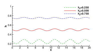
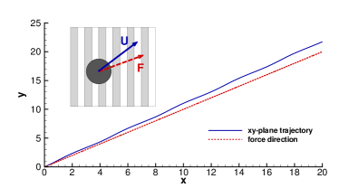
Figure 8: Trajectory in the $xh$ plane (top panel) for a particle of radius $a=2$ released at $x_{0}=0$, $y_{0}=0$ for three different initial gaps: $h_{0}=0.25$ (dashed line), $h_{0}=0.5$ (solid line) and $h_{0}=0.75$ (dash-dotted line). The trajectory in the $xy$ for the case $h_{0}=0.25$ is reported in the bottom panel.

5.1 Constant forcing along the stripes

In the case of a constant force with vanishing wall normal component, system (9) reduces to

$$\frac{dx}{dt} = M_{11}(x,h)F_{1}$$ (10)

$$\frac{dy}{dt} = M_{22}(x,h)F_{2}\$$ (11)

$$\frac{dh}{dt} = M_{31}(x,h)F_{1}\,.$$ (12)

In Fig. 8 the $xh-$ and $xy-$projection of a typical trajectory are reported, top and bottom panel, respectively. The finite mobility coefficient $M_{31}$ couples a wall-normal motion to the wall-parallel force component $F_{1}$ acting along the stripe normal. The wall normal motion occurs in periodic fashion with no mean drift. Typically, the oscillation amplitude is quite small, as expected given the small values of $M_{31}$. The motion in the wall-parallel plane $xy$ occurs at an average angle to the force direction, here oriented $45^{\circ}$ from the stripe normal (x-direction). Both mean deflection and wall-normal oscillations are clearly induced by the alternating pattern of perfect- and no-slip stripes at the solid wall.

The mean deflection observed in Fig. 8 is worth being investigated in more detail, given its potential interest for particle separation. The deflection is measured by the average trajectory slope $m=\langle dy/dx\rangle$, where angular brackets denote averaging over the spatial period $\lambda$ of the stripes. The slope $m$ is reported in Fig. 9 (top panel) for different particle radii $a$ and initial positions $(0,0,h_{0})$ for a $45^{\circ}$ inclination of the force, $F_{2}/F_{1}=1$. The behavior illustrated in the figure is generic and does not depend on the force inclination nor on the particle initial position along the stripe pattern. By inspection of the data the deflection increases as the gap $h$ is reduced and as the particle radius $a$ is augmented. This not trivial behavior is induce by the elliptic nature of the Stokes equations. However, its physical interpretation can be at least sketched for particles with radius much smaller the the stripe width, $a\ll\lambda$. Far from the border between perfect- and no-slip regions, the small particle experiences a locally isotropic wall (i.e. $M_{11}=M_{22}$), implying no deflection. However, in a region of characteristic size $\epsilon\propto a$ straddling the border, $M_{11}$ and $M_{22}$ differ significantly inducing a local deflection of the particle path. The overall deflection is somehow a weighted average between the non deflecting portions of the trajectory and the deflection regions located at the stripe borders. By increasing the particle radius $a$, the size of the non deflecting portions decreases. At the same time the deflecting effect of the border gets stronger, since it scales only with the ratio $a/h$ under the assumption $a\ll\lambda$. It follows that the overall deflection increases with $a$. This argument, even though strictly valid only in the limit $a\ll\lambda$, can provide a guideline in interpreting the general behavior.

Clearly the amount of deflection does indeed depend on the forcing directions and vanishes for forces perfectly normal or parallel to the stripes. In any case, the maximum deflection turns out to be small, at most a few percent with respect to the forcing angle. This finding is consistent with similar results discussed in [32] where molecular dynamics is used to compute the trajectory of a particle dragged by the underlying flow and in [33] where a Poiseuille flow over a patterned wall is considered.

Given the slope of the particle trajectory in the xy plane,

$$\frac{dy}{dx}=\frac{M_{22}(x,h)}{M_{11}(x,h)}\frac{F_{2}}{F_{1}}\,,$$ (13)

a rough approximation for the average slope based on the small oscillations of $h(x)$ is

$$m=\left\langle\frac{dy}{dx}\right\rangle\simeq\left\langle\frac{M_{22}(x,h_{0})}{M_{11}(x,h_{0})}\right\rangle\frac{F_{2}}{F_{1}}\,.$$ (14)

The above estimate corresponds quite well to the actual data, as shown in Fig. 9 (top panel) by the comparison of symbols and dashed lines. Significant discrepancies become apparent for small gaps $h_{0}$, where $M_{31}(x,h)$ becomes significant (see Fig. 7) and the wall-normal oscillation is no more negligible, see the top panel of Fig. 8.

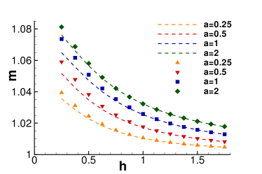
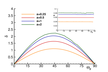
Figure 9: Top panel: Observed (symbols) and predicted (dashed lines) average slopes $m$ for particles driven by a $45^{\circ}$ constant forcing $F_{2}/F_{1}=1$ as function of the initial gap $h_{0}$. Bottom panel: Absolute deflection $\delta$ (degrees) with respect to the forcing angle $\Theta_{F}$ for $h_{0}=0.25$. The $45^{\circ}$ forcing achieves the maximum absolute deflection for a given radius. In the inset, measured relative difference between the actual trajectory slope $m$ and tangent of the forcing angle slope $m_{F}=F_{2}/F_{1}$, $s=(m-m_{F})/m_{F}$.

The bottom panel of Fig. 9 shows the absolute angular deflection $\delta=\Theta-\Theta_{F}$ with $\Theta=\tan^{-1}(m)$ and $\Theta_{F}=\tan^{-1}(m_{F})$, where $m_{F}=F_{2}/F_{1}$. A maximum angular deflection is apparent for $\Theta_{F}=45^{\circ}$ while, as expected by symmetry consideration, $\delta=0$ for $\Theta_{F}=0^{\circ}$ (perpendicular to the stripes) and $\Theta_{F}=90^{\circ}$ (parallel). Interestingly, defined the relative slope difference

$$s=\frac{m-m_{F}}{m_{F}}\,,$$ (15)

eq. (14) implies that $s\simeq\langle M_{22}(x,h_{0})/M_{22}(x,h_{0}\rangle-1$, i.e. $s$ does not depend on the direction of the applied force. This is consistent with the data reported in the inset of the bottom panel of Fig. 9.

5.2 Spatially periodic forcing along the stripes

When the transverse force component $F_{2}$ is an oscillating function of the coordinate $x$ normal to the stripes, certain resonance effects may emerge. To address the problem, one may exploit system (10-12) by noticing that the equations for $x(t)$ and $h(t)$ are $y$-independent. Hence the system can be first solved for the unknowns $x(t)$ and $h(t)$ for a constant force $F_{1}=1$, $F_{3}=0$, as in § 5.1. The solution of eq. (11) then provides $y(t)=y[t;x,h,F_{2}]$ as a functional of $x(t),h(t)$ and $F_{2}(x)$. This functional is linear in $F_{2}(x)$. The average deflection of the particle along the stripes per wavelength of wall pattern will then depend on amplitude and shape of $F_{2}(x)$. The force distribution can be optimized to maximize the particle drift for given physical constraints, e.g. periodic, zero average force $\langle F_{2}\rangle=0$ and prescribed effective amplitude $A=\sqrt{\langle F_{2}^{2}\rangle}$. It is not difficult to show that the solution of the optimization problem is

$$F_{2}^{opt}(x)=A\frac{\frac{\displaystyle M_{22}\left[x,h(x)\right]}{\displaystyle M_{11}\left[x,h(x)\right]F_{1}}-\frac{\displaystyle 1}{\displaystyle\lambda}\left\langle\frac{\displaystyle M_{22}}{\displaystyle(M_{11}F_{1})}\right\rangle}{\sqrt{\left\langle\left(\frac{\displaystyle M_{22}}{\displaystyle M_{11}F_{1}}\right)^{2}\right\rangle-\frac{\displaystyle 1}{\displaystyle\lambda}\left\langle\frac{\displaystyle M_{22}}{\displaystyle M_{11}F_{1}}\right\rangle^{2}}}\,,$$ (16)

where $h(x)=h\left[t(x)\right]$ with $t(x)$ the inverse of $x(t)$. From eq. (13) the optimized slope follows as

$$m^{opt}=\frac{A}{\lambda F_{1}}\sqrt{\left\langle\frac{M_{22}}{M_{11}F_{1}}^{2}\right\rangle-\frac{1}{F_{1}\lambda}\left\langle\frac{M_{22}}{M_{11}F_{1}}\right\rangle^{2}}\ .$$ (17)

Instead of using the solution of the optimization problem, in the following $F_{2}(x)$ is taken to be a sinusoid,

$$\frac{dy}{dt}=M_{22}(x,h)\frac{A}{\sqrt{2}}\sin\left(\frac{2\pi x}{\lambda}\right)\,,$$ (18)

a simple shape that is, in many cases, not too far from the optimal. Indeed, at least for trajectories not too close to the surface, the two mobility coefficients are reasonably well approximated by the expressions $M_{22/11}\simeq M_{22/11}^{0}+M_{22/11}^{1}\sin\left(2\pi x/\lambda\right)$, implying from eq. (16) $F_{2}^{opt}\sim\sin\left(\frac{2\pi x}{\lambda}\right)$. Figure 10 (top panel) shows the measured values of $m$ as a function of the initial gap $h_{0}$ for several sphere radii. The slope $m$ is calculated as an average along an actual trajectory, $m=\langle dy/dx\rangle$. For relatively small values of $a$ the behavior of $m$ vs $h_{0}$ is monotonic. As the sphere reaches the size $a=2$ (i.e. its diameter equals the pattern period) a new behavior emerges. This is presumably associated with the strong oscillations in $h(t)$ that occur in these conditions, related to the increased $M_{13}$. $m$ scales linearly with the amplitude of the forcing such that $m/A$ depends only on the initial gap $h_{0}$ and on the particle radius.

A rough estimate of the deflection coefficient $m$, at least for small oscillations in $h$, is

$$m=\left\langle\frac{dy}{dx}\right\rangle\simeq\left\langle\frac{M_{22}(x,h_{0})\sin({2\pi x}/{\lambda})}{M_{11}(x,h_{0})}\right\rangle\frac{A}{F_{1}}\,.$$ (19)

The results of this approximation (dashed lines) compare well with the data shown by symbols in Fig. 10 for $a<2$. At $a=2$, the accuracy is lost due to the strong oscillations in $h$ which spoil the approximation.

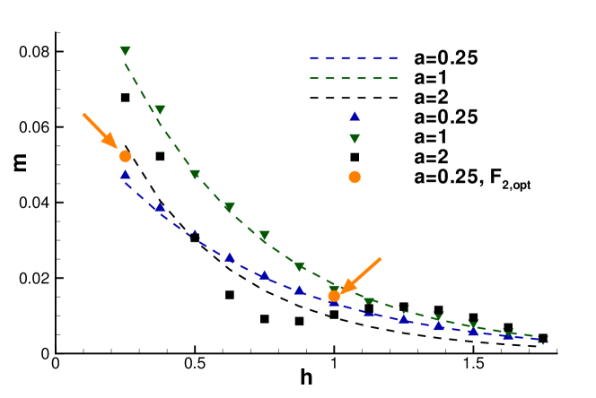
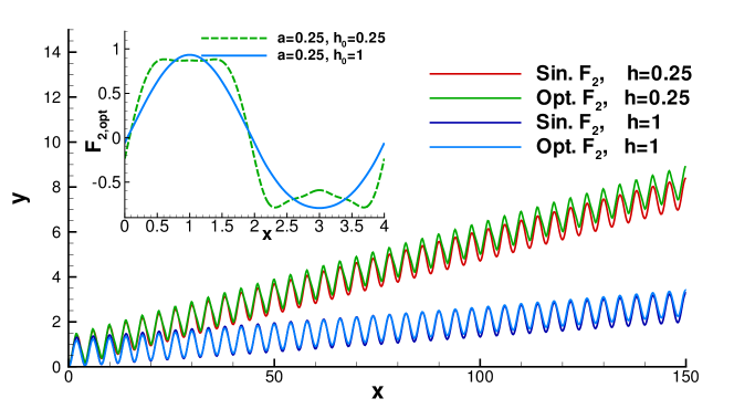
Figure 10: Top panel: observed (symbols) and predicted (dashed lines) average slopes $m$ for particles driven by a constant force in the $x$ direction ($F_{1}=1$) and $x-$dependent force in the $y-$direction (eq. 18) with $A=\sqrt{2}$ as function of the initial gap $h_{0}$. Circles are referred to average slopes $m$ obtained using the optimal forcing in the $y-$direction (eq. 16). Bottom panel: comparison of trajectories obtained by sinusoidal and optimal forcing in the $y-$direction. The top curve pair compares the trajectories at $h=0.25$. The bottom pair provides the comparison at $h=1$, where the two curves are almost superimposed. The inset shows $F_{2}^{opt}(x)$ (eq. 16) for two values $h_{0}=0.25,1$.

As a last remark, the trajectory under the optimal force $F_{2}^{opt}(x)$, eq. (16), is compared to the results with the sinusoidal force, bottom panel of figure 10 for $a=0.25$. Two cases are considered, namely $h_{0}=0.25$ and $h_{0}=1$. As expected, far from the wall, i.e. at $h_{0}=1$, the two forces are almost equivalent. In the near wall region the optimal force is indeed slightly more effective in maximizing the drift. The shape of the optimal force is compared for the wall-distances $h_{0}=0.25$ and $1$ in the inset of Fig. 10. At large distance the optimal force approaches a sinusoid, while substantial differences are found closer to the wall where the optimal shape resembles a square-wave consistently with the discontinuous boundary conditions enforced at surface. Even in this case the comparison of the trajectories confirms that the sinusoid is nearly optimal in maximizing the drift. The drift coefficients $m$ under optimal forcing are reported in the top panel of figure 10 as filled circles highlighted by arrows.

It might be interesting to specialize the traction force $F_{1}$ for the very common case where the force is proportional to the particle volume, $F_{1}\propto\frac{4}{3}\pi a^{3}$, like it happens, e.g., for the vertical settling of a particle under gravity. The cubic dependence on the particle radius results in a strong reduction of the velocity normal to the horizontal stripes (crossing velocity) for smaller particles. The increased crossing time $T_{c}$ leads to a larger transversal impulse $\int_{0}^{T_{c}}F_{2}dt$, thus amplifying the oscillations and the mean deflection of the particle. Indeed, the differences between small and large particle radii apparent in Fig. 11 may inspire simple particle sorting devices based on the coupling of the radius-dependent traction force with the transversal oscillating field.

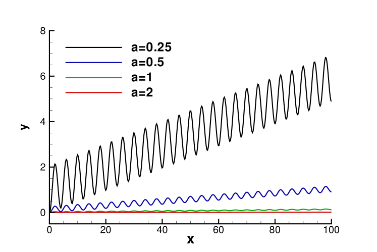
Figure 11: Trajectories obtained for a sinusoidal forcing (eq. 18) for different particle radii, when the external force $F_{1}$ in the stripe-normal direction is proportional to the particle volume like, e.g. in the case of the gravity force. The smaller the particle, the slower its stripe-normal motion (curves from top to bottom correspond to particles with increasing radii): the transversal force $F_{2}$ acts for a longer time on the smaller spheres producing larger oscillations amplitudes and mean deflection in the trajectory.

5.3 Time dependent forcing along the stripes

The previous section showed that significant mean particle drifts can be achieved by an oscillating spatial distribution of the transverse force. This finding suggests to look at the effect of a time-oscillating space-homogeneous transverse force $F_{2}(t)$. As in the previous section the particle is pulled along the $x$ direction by a constant force $F_{1}=1$ with a superimposed transverse oscillating forcing with zero mean. The resulting equation for the transverse motion of the particle is

$$\frac{dy}{dt}=M_{22}(x,h)B\sin\left(\frac{2\pi t}{T}\right)\,,$$ (20)

to be solved together with equations (10) and (12).

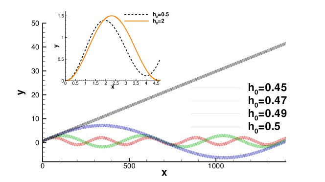
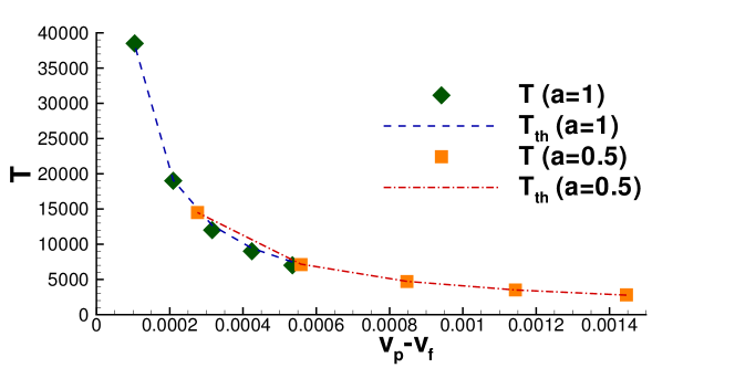
Figure 12: Top panel: trajectory in the $x-y$ for the sphere of radius $a=1$ released at several wall normal initial positions $h_{0}$ which ranges from $0.5$ (straight line) to $0.45$ (higher frequency curve). Inset: close up view of the trajectory at the initial stages. Bottom panel: the fast oscillation period of $y[x(t)]$ (symbols) is compared with the model estimate (dashed line, eq.22) as a function of the velocity difference $(v_{p}-v_{f})$.

In the top panel of Fig. 12 different $xy$ trajectories are reported for $a=1$, $B=1$, different initial positions $(0,0,h_{0})$ and $T=114$. The trajectory is characterized by two different wave-lengths. The shortest one is not appreciated on the scale of the plot, see the close-up in the inset. The long wavelength behavior strongly depends on the initial gap $h_{0}$ and dominates the large scale motion. Its spatial period progressively increases as $h_{0}$ approaches the critical value $h_{c}=0.5$ where the periodicity is lost (infinite oscillation period) and the particle drifts steadily. In this limiting conditions the trajectory degenerates in a rectilinear motion with superimposed the aforementioned small scale oscillations. The observed behavior can be understood in terms of a simplified model amenable of analytical solution. The model adopts a few assumptions that are reasonably well justified by the results described in the previous sections. A first simplification consists in freezing the $h$ dependence of the mobility coefficient $M_{22}(x,h)\simeq M_{22}(x,h_{0})$. Successively, the $x$ dependence is approximated by its dominating Fourier modes $M_{22}(x,h_{0})\simeq\overline{M}_{22}+b_{1}\sin\left(\frac{2\pi}{\lambda}x\right)$, where $\overline{M}_{22}$ and $b_{1}$ are mean value and first harmonic amplitude, respectively. Finally the motion along the $x$ direction under the action of the constant force $F_{1}$ is roughly approximated as $x(t)=v_{p}t+x_{0}$, where $v_{p}$ is the mean cross-stripe particle velocity. Equation  (20) than becomes

$$\frac{dy}{dt}=\left\{\overline{M}_{22}+b_{1}\sin\left[\frac{2\pi}{\lambda}\left(v_{p}t+x_{0}\right)\right]\right\}B\sin\left(\frac{2\pi t}{T}\right)\ .$$ (21)

The solution follows as

$$y(t) = \frac{B\lambda b_{1}}{2\pi(v_{p}-v_{f})}\sin\left(\frac{2\pi}{\lambda}(v_{p}-v_{f})t+\phi\right)$$ (22)

$$- \frac{B\lambda b_{1}}{2\pi(v_{p}+v_{f})}\sin\left(\frac{2\pi}{\lambda}(v_{p}+v_{f})t+\phi\right)$$ (23)

$$- \frac{B\overline{M}_{22}\lambda}{2\pi v_{f}}\cos\left(\frac{2\pi}{\lambda}v_{f}t\right)+y_{0}$$ (24)

where $\phi=2\pi x_{0}/\lambda$ is the initial phase. In the above expression $v_{f}=\lambda/T$ is a characteristic velocity of the system fixed by the wall pattern spacing $\lambda$ and the forcing period $T$. The time dependence of $y(t)$ results from the superimposition of three signals with different frequencies. The fundamental frequency is determined by the forcing period, term (24), and the corresponding amplitude is proportional to the transverse mean mobility $\overline{M}_{22}$. This fundamental contribution remains the only relevant one far from the wall, where the $x$-dependence of $M_{22}$ becomes negligible (vanishing $b_{1}$), i.e. the surface effectively behaves as a homogeneous wall. The two sideband contributions, (22) and (23), follow from the interaction between the forcing frequency and the surface pattern, as shown by their proportionality to the transverse forcing amplitude $B$ and to the first Fourier coefficient of the pattern $b_{1}$. For particles advancing in the positive $x$-direction ($v_{p}>0$), the first side-band term (22) is the more interesting one, since by proper tuning the relative velocity $v_{p}-v_{f}$ can be made to vanish. The other side-band term, (23), is typically irrelevant since its amplitude is too small to be detected in comparison with the fundamental contribution given that, in general, $\overline{M}_{22}\gg b_{1}$. For this reason such small oscillations can not be observed in Fig. 12. Concerning the first side-band term, in the limit $v_{p}-v_{f}\to 0$ its amplitude diverges while at the same time the frequency $2\pi(v_{p}-v_{f})/\lambda$ vanishes, yielding the limiting behavior

$$\lim_{v_{p}-v_{f}\to 0}y(t)=\frac{1}{2}Bb_{1}t\,.$$ (25)

This term, combined with $x(t)=v_{p}t+x_{0}$, gives reason of the (average) rectilinear trajectory of Fig. 12 that occurs when the initial condition $h_{0}$, $x_{0}$ selects a mean particle velocity $v_{p}(h_{0},x_{0})$ matching the system characteristic velocity $v_{f}$. Such case corresponds to resonance, since the particle exactly travels one wall pattern wave-length $\lambda$ in one oscillation period $T$ of the transversal force. In these conditions a strong amplification of the particle transversal motion occurs. To complete the discussion, the bottom panel of Fig. 12 shows the period of the fast oscillations of the in-plane trajectory $y[x(t)]$ as a function of the velocity difference $(v_{p}-v_{f})$. Also reported are the corresponding values from the model system, term (22). The comparison confirms the overall effectiveness of the simplified model.

6 Conclusion

The paper exploited the potential of the Boundary Element Method (BEM) in the context of creeping flows in the Stokes regime. In a number of applications at the micro-scales the fluid boundary condition at solid walls is best described by a perfect-slip or partial slip boundary condition. The BEM proved successful in dealing with such complex surfaces characterized by a combination of perfect-slip (PS) and no-slip (NS) regions. In the geometry addressed in the present paper, the PS regions on the wall form a parallel-striped pattern able to effectively model an actual superhydrophobic surface where gas bubbles are trapped in parallel grooves.

In this context the hydrodynamics of a spherical particle moving close to the patterned surface has been characterized in terms of the mobility tensor. The wall pattern induces a characteristic spatial behavior of the mobility. Different regions have been identified. As expected, near the wall the mobility is larger in correspondence of the PS regions than in correspondence of the NS regions. In contrast, in the far field this behavior is reversed, i.e. the mobility becomes (slightly) larger when the sphere is just above a NS region. The modulation effects induced by the patterning become progressively weaker increasing the distance from the wall. In the far field the oscillation in $M_{11}$ is less than $5\%$ of the average value $\overline{M}_{11}$. The wall normal distance $h_{inv}$ that separates the two regimes decreases with the sphere radius. Interestingly, irrespectively of the particle radius, the average mobility $\overline{M}_{11}$ for a given gap $h$ is well described by an effective model consisting of a homogeneous wall equipped with a partial slip boundary condition accounting for an effective slip-length, see e.g [7, 4]. The present results provide solid physical ground for the safe application of analytical models based on homogenization techniques [34]. This behavior is particularly evident for large particles (diameter larger than the stripe dimension) where the far field regime sets in very close to the wall. It follows that, with the exception of a very thin area ($h<h_{inv}$), the mobility field is well approximated by the effective wall model.

The characteristic spatial dependence of the mobility matrix can be potentially exploited for selective particle separation, as confirmed by simple numerical experiments. For instance, towing the sphere with a constant force in a wall parallel plane leads to a deviation of the trajectory. The resulting drift angle is in agreement with results discussed in [32] in the context of molecular dynamics simulations. Larger drift angles can be achieved by other kind of forcing, as in the case of a spatially or temporally oscillating force parallel to the stripes. In the second case in particular, a strong resonant effect occurs when the stripe-crossing frequency matches the external forcing frequency. This effect allows in principle to separate given particles from their neighbors.

As a final comment it is worth stressing that the model here described for the superhydrophobic surfaces relies on the assumption of a flat liquid-gas meniscus (PS region). A number of studies show that this is hardly strictly true also in simple systems [35, 36, 37, 38]. However, the present results show that a detailed description of the surface pattern is not required unless the particle is very close to the wall. Indeed it was shown that it is actually often sufficient to model the surface as a homogeneous flat wall with a suitable apparent slip length tensor. In this effective description the curvatures of the menisci enters the problem by affecting the apparent slip-length, see e.g.[39, 40, 12]. Still it should not be overlooked that the near wall behavior is dominated by the local effects emphasizing the role of the actual shape of the liquid/gas interface. The BEM approach here used can easily be extended to tackle such conditions to deal with composite boundaries on which perfect-slip, no-slip and partial slip boundary conditions are imposed. This opens the way to the characterization of more complex systems such as slipping Janus particles motion [41] and micro-swimmers [42, 43].

Appendix A Boundary integral formulation

In this section the application of the Boundary Element Method (BEM) to the present geometrical configuration is shortly described, see e.g. [24, 23] for further details.

Due to linearity, the constant coefficient Stokes problem, eq. (2), can be recast into a boundary integral representation formula

$$E(\mbox{\boldmath$\xi$})u_{j}(\mbox{\boldmath$\xi$}) = \frac{1}{8\pi}\int_{\partial B}t_{i}({\bf x})G_{ij}({\bf x},\mbox{\boldmath$\xi$})\,dS_{B}$$ (26)

$$- \frac{1}{8\pi}\int_{W_{NS}}t_{i}({\bf x})G_{ij}({\bf x},\mbox{\boldmath$\xi$})\,dS_{NS}$$

$$- \frac{1}{8\pi}\int_{W_{PS}}t_{i}({\bf x})G_{ij}({\bf x},\mbox{\boldmath$\xi$})\,dS_{PS}$$

$$- \frac{1}{8\pi}\int_{\partial B}u_{i}({\bf x}){\cal T}_{ijk}({\bf x},\mbox{\boldmath$\xi$})n_{k}({\bf x})\,dS_{B}$$

$$- \frac{1}{8\pi}\int_{W_{NS}}u_{i}({\bf x}){\cal T}_{ijk}({\bf x},\mbox{\boldmath$\xi$})n_{k}({\bf x})\,dS_{NS}$$

$$- \frac{1}{8\pi}\int_{W_{PS}}u_{i}({\bf x}){\cal T}_{ijk}({\bf x},\mbox{\boldmath$\xi$})n_{k}({\bf x})\,dS_{PS}.$$

In equation (3) the boundary $\partial\Omega$ of the fluid domain is explicitly decomposed in three parts: the particle surface $\partial B$, the no-slip stripes on the patterned wall, collectively denoted $W_{NS}$, and the complementary part of the wall with the perfect slip stripes $W_{PS}$. The contributions arising from the portion of the boundary at infinity (not included in the present formulation where the fluid is assumed to be at rest) can be easily incorporated under suitable assumption on the asymptotic behavior of the field. The effects of body forces like gravity or electric fields can be accounted for by a convolution integral extended to the fluid domain between the force and the free space Green’s tensor (see below). In representation (26), $t_{i}$ and $u_{i}$, $i=1,\ldots,3$, are the Cartesian components of the surface stress and velocity, respectively. The free space Green’s function (the so-called steady Stokeslet) is defined as

$$G_{ij}({\bf r})=\left(\frac{\delta_{ij}}{r}+\frac{r_{i}r_{j}}{r^{3}}\right)\,,$$ (27)

and the associated stress tensor is

$${\cal T}_{ijk}({\bf r})=-6\frac{r_{i}r_{j}r_{k}}{r^{5}}.$$ (28)

In the above expression, $G_{ij}({\bf r})$ provides the contribution to the j-th velocity component at $\xi$ due to a concentrated force acting in the i-th direction at ${\bf x}$. The associated Green’s stress tensor, as always, should be contracted with the outward unit normal $n_{k}({\bf x})$ to the boundary $\partial\Omega$ in order to provide the effect on the j-th velocity component at $\xi$ of the i-th boundary velocity at ${\bf x}$. The vector ${\bf r}$ is defined as ${\bf r}={\bf x}-\mbox{\boldmath$\xi$}$ with $r=\sqrt{r_{k}r_{k}}$ its modulus. In eq. (3) $E(\mbox{\boldmath$\xi$})=1$ when $\mbox{\boldmath$\xi$}\in\Omega$ and $E(\mbox{\boldmath$\xi$})=1/2$ for $\mbox{\boldmath$\xi$}\in\partial\Omega$ (the existence of a regular tangent plane is assumed throughout). When $\mbox{\boldmath$\xi$}\in\partial\Omega$, representation (3) becomes a boundary integral equation where the unknowns can either be the three stress vector components $t_{i}$, the three velocity components $u_{i}$, or a combination thereof, depending on the boundary conditions assigned on the specific portion of boundary. This approach allows to discretize only the boundary surfaces of the flow domain instead of considering the entire volume. This results in: 1) a substantial reduction of the number of unknowns; 2) the possibility to easily specify different kinds of boundary condition on different surface patches; 3) the simple update of the geometry when dealing with time dependent configurations. Once the boundary $\partial\Omega$ is discretized into panels, eq. (3) is recast into an algebraic linear system whose solution can be achieved by standard linear algebra packages. In simple cases, part of the boundary can be accounted for by symmetry, like it happens for a flat homogeneous wall.

In this paper, given the generality of the boundary condition to be used at the wall (either patterned perfect/no-slip stripes or effective slip Navier-like boundary conditions) the complete formulation of the boundary integral problem based on the free-space Green’s function has been retained, with the use of the wall Green’s function demanded of providing reference results for accuracy tests.

Finally, a few more words may be useful as concerning the specific boundary conditions used in the paper. On the perfect-slip boundary patches, $W_{PS}$, the normal velocity vanishes $u_{\perp}=0$ due to impermeability while the tangential velocity ${\bf u}_{\parallel}$ (two Cartesian components) is unknown. Moreover, the tangential stress ${\bf t}_{\parallel}$ vanishes by perfect slip such that the stress is aligned to the normal, $t_{i}=-\Phi({\bf x})n_{i}$, with $\Phi$ representing a further scalar unknown. On the no-slip surfaces, $W_{NS}$ and $\partial B$, velocities are completely assigned while stresses are unknown. Concerning the partial slip condition used as an effective model of the stripe pattern, zero normal velocity $u_{\perp}=0$ at the wall are implied, while tangential velocities and stresses are coupled by the Navier condition [44],

$${\bf u}_{\parallel}=\vec{\ell_{s}}\vec{n}\cdot(\vec{\nabla}{{\bf u}}+(\vec{\nabla}{{\bf u}})^{T})\cdot(\vec{1}-\vec{n}\otimes\vec{n})\ .$$ (29)

Here $\vec{\ell_{s}}$ is a $2\times 2$ symmetric [45] tensor describing the directionally dependent slip-length. In the present case this tensor is diagonalized when expressed in stripe-parallel and stripe-normal Cartesian coordinates. In this case the two diagonal entries are different as a consequence of the orientation of the stripe pattern. For a flat wall eq. (29) is rewritten as

$$\vec{u}_{\parallel}=\vec{\ell_{s}}\cdot\vec{t_{\parallel}}\,,$$ (30)

that is the vectorial form of eq. (7), the two non-zero components of $\vec{\ell_{s}}$ being reported in eq. 8 [7, 4]. The boundary integral equation (3) supplemented with eq. (30) provides a closed system that after inversion determines all the unknowns involved in the problem.

References

- [1] M. Nosonovsky, B. Bhushan, Current Opinion in Colloid & Interface Science 14(4), 270 (2009)
- [2] F. Bottiglione, G. Carbone, Langmuir 29(2), 599 (2012)
- [3] C. Ybert, C. Barentin, C. Cottin-Bizonne, P. Joseph, L. Bocquet, Physics of fluids 19, 123601 (2007)
- [4] C. Ng, C. Wang, Microfluidics and Nanofluidics 8(3), 361 (2010)
- [5] C. Lee, C. Kim, Langmuir: the ACS journal of surfaces and colloids 27(7), 4243 (2011)
- [6] O.I. Vinogradova, A.V. Belyaev, Journal of Physics: Condensed Matter 23(18), 184104 (2011)
- [7] J. Philip, Zeitschrift für Angewandte Mathematik und Physik (ZAMP) 23(3), 353 (1972)
- [8] Z. Li, Physical Review E 80(6), 061204 (2009)
- [9] M. Chinappi, S. Melchionna, C.M. Casciola, S. Succi, The Journal of Chemical Physics 129, 124717 (2008)
- [10] R. Benzi, L. Biferale, M. Sbragaglia, S. Succi, F. Toschi, EPL (Europhysics Letters) 74, 651 (2006)
- [11] C. Cottin-Bizonne, C. Barentin, É. Charlaix, L. Bocquet, J. Barrat, The European Physical Journal E: Soft Matter and Biological Physics 15(4), 427 (2004)
- [12] D. Gentili, M. Chinappi, G. Bolognesi, A. Giacomello, C. Casciola, Meccanica pp. 1–9 (2013)
- [13] M. Chinappi, F. Gala, G. Zollo, C.M. Casciola, Philosophical Transactions of the Royal Society A: Mathematical, Physical and Engineering Sciences 369(1945), 2537 (2011)
- [14] M. Chinappi, C.M. Casciola, Physics of Fluids 22, 042003 (2010)
- [15] D. Huang, C. Sendner, D. Horinek, R. Netz, L. Bocquet, Physical review letters 101(22), 226101 (2008)
- [16] H. Zhang, Z. Zhang, H. Ye, Microfluidics and Nanofluidics pp. 1–9 (2012)
- [17] L. Zhu, C. Neto, P. Attard, Langmuir 28(20), 7768 (2012)
- [18] C. Cottin-Bizonne, A. Steinberger, B. Cross, O. Raccurt, E. Charlaix, Langmuir 24(4), 1165 (2008)
- [19] Y. Pan, B. Bhushan, Journal of Colloid and Interface Science (2012)
- [20] O.I. Vinogradova, Langmuir 11(6), 2213 (1995)
- [21] A.V. Belyaev, O.I. Vinogradova, Journal of Fluid Mechanics 652, 489 (2010)
- [22] J.R. Happel, H. Brenner, Low Reynolds number hydrodynamics: with special applications to particulate media, vol. 1 (Springer, 1965)
- [23] S. Kim, S. Karrila, Microhydrodynamics: principles and selected applications (Dover Publications, 2005)
- [24] C. Pozrikidis, Boundary integral and singularity methods for linearized viscous flow. 8 (Cambridge University Press, 1992)
- [25] J.F. Brady, G. Bossis, Annual review of fluid mechanics 20, 111 (1988)
- [26] C. Pozrikidis, A practical guide to boundary element methods with the software library BEMLIB (CRC, 2002)
- [27] J. Blake, in Proc. Camb. Phil. Soc, vol. 70 (Cambridge Univ Press, 1971), vol. 70, pp. 303–310
- [28] L. Landau, Fluid Mechanics: Volume 6 (Course Of Theoretical Physics) Author: LD Landau, EM Lifshitz, Publisher: Bu (Butterworth-Heinemann, 1987)
- [29] A. Goldman, R.G. Cox, H. Brenner, Chemical Engineering Science 22(4), 637 (1967)
- [30] G. Batchelor, Journal of Fluid Mechanics 74(01), 1 (1976)
- [31] D. Jeffrey, Y. Onishi, Journal of Fluid Mechanics 139(1), 261 (1984)
- [32] R. Zhang, J. Koplik, Physical Review E 85(2), 026314 (2012)
- [33] J. Zhou, A.V. Belyaev, F. Schmid, O.I. Vinogradova, The Journal of Chemical Physics 136(19), 194706 (2012). DOI 10.1063/1.4718834. URL http://link.aip.org/link/?JCP/136/194706/1
- [34] E.S. Asmolov, A.V. Belyaev, O.I. Vinogradova, Physical Review E 84(2), 026330 (2011)
- [35] A. Steinberger, C. Cottin-Bizonne, P. Kleimann, E. Charlaix, Nature materials 6(9), 665 (2007)
- [36] A. Giacomello, S. Meloni, M. Chinappi, C.M. Casciola, Langmuir 28(29), 10764 (2012)
- [37] A. Giacomello, M. Chinappi, S. Meloni, C.M. Casciola, Physical Review Letters 109(22), 226102 (2012)
- [38] G. Bolognesi, C. Pirat, E. Cottin-Bizonne, M. Guene, J. Teisseire, Soft Matter (Under Review)
- [39] C. Teo, B. Khoo, Microfluidics and Nanofluidics 9(2), 499 (2010)
- [40] M. Sbragaglia, A. Prosperetti, Physics of Fluids 19, 043603 (2007)
- [41] A.M. Boymelgreen, T. Miloh, Physics of Fluids 23, 072007 (2011)
- [42] H. Shum, E. Gaffney, Physics of Fluids 24, 061901 (2012)
- [43] L. Zhu, E. Lauga, L. Brandt, Journal of Fluid Mechanics 726 (2013)
- [44] E. Lauga, M. Brenner, H. Stone. Handbook of experimental fluid mechanics (2007)
- [45] K. Kamrin, M.Z. Bazant, H.A. Stone, Journal of Fluid Mechanics 658, 409 (2010)