Collapse of superhydrophobicity on nanopillared surfaces

Abstract

The mechanism of the collapse of the superhydrophobic state is elucidated for submerged nanoscale textures forming a three-dimensional interconnected vapor domain. This key issue for the design of nanotextures poses significant simulation challenges as it is characterized by diverse time and length scales. State-of-the-art atomistic rare events simulations are applied for overcoming the long timescales connected with the large free energy barriers. In such interconnected surface cavities wetting starts with the formation of a liquid finger between two pillars. This break of symmetry induces a more gentle bend in the rest of the liquid-vapor interface, which triggers the wetting of the neighboring pillars. This collective mechanism, involving the wetting of several pillars at the same time, could not be captured by previous atomistic simulations using surface models comprising a small number of pillars (often just one). Atomistic results are interpreted in terms of a sharp-interface continuum model which suggests that line tension, condensation, and other nanoscale phenomena play a minor role in conditions close to coexistence.

I Introduction

Superhydrophobicity stems from the presence of a gaseous layer between a body of liquid and a surface. This suspended “Cassie” state is fostered by surface roughness and hydrophobic coatings Lafuma and Quéré (2003); the composite liquid-gas-solid interface results in important properties for submerged and “dry” technological applications, such as self-cleaning, enhanced liquid repellency, and drag reduction Quéré (2008); Rothstein (2010). The superhydrophobic Cassie state is sustained by capillary forces, which can be overcome by variations in the liquid pressure, temperature, or other external forces which trigger the transition to the fully wet Wenzel state. Thus, the design of textured surfaces and coatings has the aim of realizing a robust Cassie state.

The stability of the Cassie state depends not only on the thermodynamic conditions but also on the surface geometry and chemistry, which can be engineered in order to achieve robust superhydrophobicity. Hydrophobic textures of nanometric size Martines et al. (2005); Verho et al. (2012) proved efficient in stabilizing the gaseous layer over a broad range of pressures and temperatures Checco et al. (2014). However, the engineering of surface nanotextures is still in its infancy: understanding the collapse mechanism – i.e., the path followed by the liquid front during the breakdown of the Cassie state – is the key to improve the performance and robustness of such textures. For instance, it is possible to modify surfaces in order to destabilize the Wenzel state Prakash et al. (2016) or to achieve robust superhydrophobicity via complex nanotextures Amabili et al. (2015). Nucleation of gas and vapor bubbles, which is enhanced by surface textures Giacomello et al. (2013), can also bring to the breakdown of the Cassie state and superhydrophobic surfaces must be engineered to prevent it. However, to date the collapse mechanism on experimentally and technologically relevant textures remains largely unknown, with the theoretical approaches making a priori assumptions or being often affected by simulation artifacts as discussed in details below.

Due to their simplicity, surfaces decorated with pillars are a paradigm in the study of superhydrophobicity, both via experiments and simulations. In addition, thanks to the reduced liquid-solid contact these kind of textures favor the emergence of large slip at the walls Ybert et al. (2007), making them attractive, e.g., for drag-reduction Rothstein (2010). The focus of this work is the wetting of 3D submerged nanopillars (Fig. 1): the three distinctive attributes of the textured studied in this work are submerged, three-dimensional, and nanoscale. Indeed, most simulations to date have restricted their attention to drops of sizes comparable to that of the texture at the top of which they are sitting Dupuis and Yeomans (2005); Kusumaatmaja and Yeomans (2007); Koishi et al. (2009); Savoy and Escobedo (2012a); Ren (2014); Zhang and Ren (2014); Pashos et al. (2015); in this setup the collapse mechanism is significantly influenced by the drop shape and size. At variance with drops, the main issue for submerged surfaces is the resistance of the superhydrophobic state against pressure variations Giacomello et al. (2012a); Savoy and Escobedo (2012b); Amabili et al. (2015, 2016); Prakash et al. (2016). Present superhydrophobic surfaces generally exhibit complex 3D morphologies with isolated (pores) or connected (pillars, cones) cavities. Two-dimensional or quasi-2D (limited thickness) models have been often used in simulations with the aim of reducing their computational cost Savoy and Escobedo (2012a, b); Giacomello et al. (2012a); Amabili et al. (2015); Pashos et al. (2015). However, systems such as pillared surfaces cannot be reduced to 2D without overlooking important phenomena, e.g., the simultaneous wetting of several interpillar spacings. Concerning the methods, mainly due to the significant computational cost, most approaches dealing with 3D structures to date considered a continuum description of the liquid (and solid) Ren (2014); Zhang and Ren (2014); Pashos et al. (2015, 2016); Tretyakov et al. (2016); Panter and Kusumaatmaja (2017), which necessarily introduces some assumptions concerning the structure of the interfaces, the interaction with the wall, and other nanoscale effects such as fluctuations, line tension, etc. Such effects are in principle relevant on the nanoscale. In order to avoid these limitations and explore the fundamentals of wetting of experimentally relevant, 3D nanotextures, here the collapse mechanism of a large sample containing a $3$-by-$3$ array of pillars is identified via molecular dynamics (MD) combined with the string method in collective variables. Other atomistic approaches have been recently employed which, however, lead to a discontinuous dynamics for the collapse of the meniscus Prakash et al. (2016) (a detailed analysis of this problem is reported elsewhere Giacomello et al. (2015)).

In brief, the objective of this work is addressing two open questions: i) finding the most probable collapse mechanism for submerged nanopillars and computing the associated free energy profile; ii) validating simple continuum models for nanoscale wetting, identifying which bulk, interface, and line terms are relevant.

Two challenges are inherent to these problems: i) employ a model which captures the physics at the nanoscale, including fluctuations, evaporation/condensation, and line tension; ii) interpret the results in simple terms, which can be used for developing design criteria. In this work, a Lennard-Jones (LJ) fluid and solid are used to tackle i). This approach is computationally expensive, but includes all the relevant physics with minimal assumptions Evans and Stewart (2015). Concerning ii), a sharp-interface continuum model is used to interpret the atomistic results, which yields a simple and informative picture of the phenomena and allows to shed light on the nanoscale effects. Results show that, differently from previous studies focusing on independent cavities De Coninck et al. (2011); Giacomello et al. (2015), the collapse mechanism for pillars is characterized by the combination of local and collective effects. In particular, the meniscus breaks the symmetry imposed by the confining geometry and the collapse happens via the local formation of a single liquid finger followed by the correlated, collective wetting of the interpillar space of points far apart on the surface.

In interconnected geometries the meniscus is expected to assume complex morphologies during the collapse. In the present study the (atomistic) density field $\rho(\bm{x})$ is used in order to monitor the process: this choice allows one to track any changes in the meniscus shape and, at the same time, is straightforward to compute in atomistic simulations (Fig. 1). The most probable wetting path is identified via the string method by using the density field to characterize the system configuration. The identified path corresponds to a sequence of density fields $\rho(\bm{x})$ at discrete steps along the collapse process. The string method also allows for computing the free energy along the most probable path $\Omega\left(\rho(\bm{x})\right)$ and, thus, the free energy barrier determining the kinetics of the process. Indeed, we show that under ambient pressure and temperature conditions the wetting requires that the system climbs a sizable free energy barrier, which is possible only thanks to thermal fluctuations Bonella et al. (2012); Lelièvre et al. (2010).

The paper is organized in a methodological section, in which the main conceptual aspects of the string method are described, and a second, self-contained section in which the results on the collapse of the superhydrophobic state are discussed in depth. Thus, the reader interested only in the physical results can go directly to this latter section. The final section is left for conclusions.

II Methods

Typically, large free energy barriers separate the Cassie and Wenzel states. This means that, even if thermodynamics might favor the process, i.e., the final is state more stable than the initial one, the system still has to climb the free energy up to a saddle point (barrier) for the wetting transition to take place. This is different from barrierless processes; in presence of a barrier wetting is possible only thanks to thermal fluctuations, which determine the timescale for observing a transition event. This timescale is too long to be accessed by brute force MD: this is the problem of rare events Bonella et al. (2012). To cope with this issue, here the string method in collective variables (CVs) is used Maragliano et al. (2006). This method allows one to follow the infrequent process at fixed thermodynamics conditions (i.e., without increasing pressure and temperature), which implies visiting configurations characterized by high free energies and a corresponding, exponentially low probability.

CVs at the basis of the string method are a (restricted) set of observables $\{\theta_{i}(\bm{r})\}_{i=1,M}$ function of $\bm{r}$, the $3n_{f}$ dimensional vector of the fluid particles positions. CVs should correspond to the degrees of freedom which are able to characterize the system along the transition from the initial to the final state. Here we employ the coarse-grained density field, which has been used in recent works on wetting transitions Giacomello et al. (2012a, 2015) and other hydrophobicity-related phenomena Miller et al. (2007). Moreover, the density field is the cornerstone of most of meso- and macroscopic descriptions of homogeneous and heterogeneous fluids, e.g., the classical Density Functional Theory Evans (1992); Löwen (2002). Thus, the coarse-grained density is a natural CV to study the collapse of the Cassie state.

The coarse-grained density field is defined as

$$\theta_{i}(\bm{r})\equiv\theta(\bm{r},{\bm{x}}_{i})=\frac{1}{\Delta V}\sum_{j=1}^{n_{f}}\tilde{\chi}(\bm{r}_{j},{\bm{x}}_{i})$$ (1)

where $\theta(\bm{r},{\bm{x}}_{i})$ is the density at the point ${\bm{x}}_{i}$ of the discretized (or coarse-grained) ordinary space (Fig. 1b) and $\tilde{\chi}(\bm{r}_{j},{\bm{x}}_{i})$ is a smoothed approximation to the characteristic function of the volume $\Delta V$ around the point ${\bm{x}}_{i}$, with the sum at the RHS running over the $n_{f}$ fluid particles. In practice, these functions count the number of atoms in each cell in Fig. 1b. In the following, whenever possible, $\theta_{i}(\bm{r})=\theta(\bm{r},{\bm{x}}_{i})$ is replaced by the lighter notation $\theta(\bm{r},{\bm{x}})$, which denotes the CV at all points $\bm{x}_{i}$ of the discretized space, and $\rho({\bm{x}})$ a realization of this CV. Although $\theta(\bm{r},{\bm{x}})$, and analogously $\rho(\bm{x})$, is interpreted as a coarse-grained density field, we find sometimes convenient to consider it as an $M$-dimensional vector with components $\theta_{i}(\bm{r})$ ($\rho_{i}$, respectively).

Our aim is to find and characterize the most probable path $\rho({\bm{x}};\tau)$ followed by the system along the Cassie-Wenzel transition. This path represents a curve in the space of the coarse-grained density or, more visually, a series of snapshots taken at successive times $\tau$ along the wetting process. The parametrization of this curve with the time $\tau$ of the transition is unpractical in actual calculations E et al. (2007). A more convenient but equivalent parametrization is the normalized arc-length parametrization, i.e., the parametrization according to the length of the curve $\rho(\bm{x};\tau)$ at a given time $\tau$, divided by the total length of the curve: $\lambda=\int_{\rho_{C}}^{\rho(\tau)}\mathrm{d}\rho/\int_{\rho_{C}}^{\rho_{W}}\mathrm{d}\rho$, where $\rho_{C}$ and $\rho_{W}$ are the density fields corresponding to the Cassie and Wenzel states, respectively, and $\mathrm{d}{\rho}=\sqrt{\sum_{i=1,M}\left(\partial\rho({\bm{x}}_{i},\tau)/\partial\tau\right)^{2}}\mathrm{d}\tau$.

An infinite number of paths exists that bring the system from the Cassie to the Wenzel state. The objective of the string method is to find the most probable one. When the thermal energy $k_{B}T$ is low as compared to the free energy barrier the system has to overcome along the process, this path must satisfy the condition Maragliano et al. (2006) (see also the Appendix)

$$\Big{[}\hat{g}\left(\rho({\bm{x}};\lambda)\right)\nabla_{\rho}\Omega\left(\rho({\bm{x}};\lambda)\right)\Big{]}_{\perp}=0\,,$$ (2)

where $\nabla_{\rho}$ is the vector of derivatives with respect to the different components of the collective variable $\rho$, namely, the vector whose components are $\partial/\partial\rho_{i}$ with $i=1,\ldots,M$. Here, the symbol $\mathbin{\perp}$ denotes “orthogonal to the path $\rho({\bm{x}};\lambda)$”; $\Omega(\rho({\bm{x}};\lambda))$ is the Landau free energy of the coarse-grained density field $\rho({\bm{x}};\lambda)$ along the string. This free energy is in general related to the probability of observing the realization $\rho({\bm{x}})$ of the coarse grained density under the atomistic probability distribution $m({\bm{r}})$:

$$\Omega(\rho({\bm{x}}))\equiv-k_{B}T\ln p\left[\rho({\bm{x}})\right]=-k_{B}T\ln\Big{(}\int\mathrm{d}\bm{r}\;m(\bm{r})\prod_{i=1}^{M}\delta(\theta(\bm{r},{\bm{x}}_{i})-\rho({\bm{x}}_{i}))\Big{)}\;.$$ (3)

The $i$-$j$ components of the metric tensor $\hat{g}(\rho({\bm{x}}))$ in Eq. (2) read

$$g_{ij}(\rho({\bm{x}}))=\frac{\int\mathrm{d}\bm{r}\;\nabla_{\bm{r}}\theta(\bm{r},\bm{x}_{i})\cdot\nabla_{\bm{r}}\theta(\bm{r},\bm{x}_{j})\;m(\bm{r})\prod_{l=1}^{M}\delta(\theta(\bm{r},\bm{x}_{l})-\rho(\bm{x}_{l}))}{\int\mathrm{d}\bm{r}\;m(\bm{r})\prod_{l=1}^{M}\delta(\theta(\bm{r},\bm{x}_{l})-\rho(\bm{x}_{l}))}\,,$$ (4)

where $\nabla_{\bm{r}}$ denotes the $3n_{f}$-dimensional vector of the derivatives with respect to the components of the particle positions, $\partial/\partial r^{l}_{\alpha}$, with $\alpha=1,\ldots,n_{f}$ and $l=x,y,z$.

The intuitive meaning of Eq. (2) is that the component of the force $\hat{g}\left(\rho({\bm{x}};\lambda)\right)\nabla_{\rho}\Omega\left(\rho({\bm{x}};\lambda)\right)$ orthogonal to the path is zero. To give a visual interpretation, $\Omega(\rho(\bm{x}))$ should be imagined as a rough free energy landscape; a path satisfying condition (2) lies at the bottom of a valley connecting the initial and final states (free energy minima) and passes through a mountain pass (free energy saddle point).

In atomistic simulations, $\hat{g}\left(\rho({\bm{x}};\lambda)\right)$ and $\nabla_{\rho}\Omega\left(\rho({\bm{x}};\lambda)\right)$ can be estimated, for each point $\lambda$ constituting the string, by an MD governed by the following equations of motion Maragliano and Vanden-Eijnden (2006):

$$m_{\alpha}\ddot{\bm{r}}_{\alpha}=-\nabla_{\bm{r}_{\alpha}}V(\bm{r})-k\sum_{i=1}^{M}(\theta(\bm{r},{\bm{x}}_{i})-\rho({\bm{x}}_{i};\lambda))\nabla_{\bm{r}_{\alpha}}\theta(\bm{r},{\bm{x}}_{i})+\text{thermo}(T)+\text{baro}(P)\text{ ,}$$ (5)

where $m_{\alpha}$ is the mass of the $\alpha$-th particle, $\alpha=1,\ldots,n_{f}$, $V(\bm{r})$ is the interparticle potential, and $k\sum_{i=1}^{M}(\theta(\bm{r},{\bm{x}}_{i})-\rho({\bm{x}}_{i};\lambda))\nabla_{\bm{r}_{\alpha}}\theta(\bm{r},{\bm{x}}_{i})$ is a biasing force which allows the system to visit regions of the phase space around the condition $\theta(\bm{r},{\bm{x}})=\rho({\bm{x}};\lambda)$. The biasing force makes it possible to estimate the gradient of the free energy and the metric matrix of points having a very low probability (high free energy), such those near the transition state. In practice, $\hat{g}\left(\rho({\bm{x}};\lambda)\right)$ and $\nabla_{\rho}\Omega\left(\rho({\bm{x}};\lambda)\right)$ are computed as time averages along the MD of Eq. (5):

$$g_{ij}(\rho({\bm{x}};\lambda)) = {1\over t_{MD}}\int_{0}^{t_{MD}}\mathrm{d}s\;\nabla_{\bm{r}}\theta(\bm{r}(s),\bm{x}_{i})\cdot\nabla_{\bm{r}}\theta(\bm{r}(s),\bm{x}_{j})\text{ ,}$$

$${\partial\Omega\left(\rho({\bm{x}};\lambda)\right)\over\partial\rho_{i}} = -{1\over t_{MD}}\int_{0}^{t_{MD}}\mathrm{d}s\;k(\theta(\bm{r}(s),{\bm{x}}_{i})-\rho({\bm{x}}_{i};\lambda))\text{ ,}$$

with $t_{MD}$ the duration of the MD simulation and the indices $i$ and $j$ running over the $M$ coarse-graining cells.

The (improved) string method E et al. (2007) is an iterative algorithm that, starting from a first-guess path, produces the most probable path $\rho({\bm{x}};\lambda)$ satisfying Eq. (2). Here we refrain to describe the algorithm in detail summarizing only the main steps of the method. For further details the interested reader is referred to the Appendix, to the original article E et al. (2007), or to reviews Bonella et al. (2012). In the string method, the continuum path $\rho({\bm{x}};\lambda)$, with $0\leq\lambda\leq 1$, is replaced by its discrete counterpart $\{\rho({\bm{x}};\lambda_{n})\}_{n=1,L}$, with $L$ the number of snapshots used to discretize the path. The algorithm starts from a first guess of the wetting path, $\{\rho^{0}({\bm{x}};\lambda_{n})\}_{n=1,L}$, and performs an iterative minimization procedure which yields a path with zero orthogonal component of the force: $\{[\hat{g}\left(\rho({\bm{x}};\lambda_{n})\right)\nabla_{\rho}\Omega\left(\rho({\bm{x}};\lambda_{n})\right)]_{\perp}=0\}_{n=1,L}$. At each iteration, $\{\hat{g}\left(\rho({\bm{x}};\lambda_{n})\right)\}_{n=1,L}$ and $\{\nabla_{\rho}\Omega\left(\rho({\bm{x}};\lambda_{n})\right)\}_{n=1,L}$ are computed by the biased MD in Eq. (5) and are used to generate a new path. The procedure is performed until convergence is reached, i.e., when the difference in the free energy of each image between two string iterations is below a prescribed threshold (see Supplemental Material for convergence plots ).

Along the path of maximum probability one can compute the free energy profile and the associated barrier, which can in turn be related to the wetting and (dewetting) transition time $t_{CW}$ ($t_{WC}$) via the transition state theory: $t_{CW}=t^{0}_{CW}\exp[\Omega^{\dagger}_{CW}/k_{B}T]$ ($t_{WC}=t^{0}_{WC}\exp[\Omega^{\dagger}_{WC}/k_{B}T]$). In the present article, the free energy profile along the most probable wetting path is reported against the filling fraction $\Phi(\lambda_{n})=(N(\lambda_{n})-N_{C})/(N_{W}-N_{C})$, where $N(\lambda_{n})\equiv\Delta V\sum_{i}^{M}\rho(\bm{x}_{i};\lambda_{n})$ is the number of liquid particles in the yellow region of Fig. 1b at the string point $\lambda_{n}$ and $N_{C}$ and $N_{W}$ are the number of particles in the Cassie and Wenzel states, respectively. In the present calculations, $N$ and $\Phi$ are non-decreasing functions of $\lambda$ along the wetting path; thus, the filling fraction can be used as an a posteriori parametrization of the most probable wetting path $\rho({\bm{x}};\Phi)$. It is important to remark that this does not imply that $\Phi$ is a good CV for the wetting transition in interconnected textured surfaces of the type studied in this article. In fact, as shortly discussed in the next section, and more extensively in a forthcoming article, using $\Phi$ or $\theta$ as CVs leads to qualitatively different results, with those of the first CV characterized by an unphysically discontinuous path.

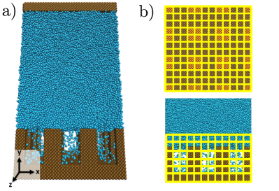
Figure 1: a) Atomistic system, consisting of a LJ fluid (blue) and solid (brown). The upper solid wall serves as a piston to impose constant pressure; the lower one is decorated with $9$ nanopillars. Temperature is controlled via a Nosé-Hoover chain thermostat Martyna et al. (1992). b) Definition of the collective variables used in the string method: coarse-grained density defined on $M=864$ cubic cells (in yellow; top and lateral views).

Summarizing, the aim of the string method in CVs is to compute the most probable path in a complex high dimensional free energy landscape. This is different from the objective and approach of other techniques (e.g., umbrella sampling, restrained MD, boxed MD, etc.), which require to reconstruct the entire landscape within a predefined volume of the CV space. The advantage of the string method is that it scales linearly with the number of CVs, while more standard methods scale exponentially. This allowed us to investigate the collapse mechanism in the high dimensional space (864 degrees of freedom) of the coarse grained density field, which would have been impossible with other approaches.

MD simulations for computing $\{\hat{g}\left(\rho({\bm{x}};\lambda_{n})\right)\}_{n=1,L}$ and $\{\nabla_{\rho}\Omega\left(\rho({\bm{x}};\lambda_{n})\right)\}_{n=1,L}$ are performed at constant pressure, temperature, and number of particles Note (2). The LJ fluid is characterized by a potential well of depth $\varepsilon$ and a length scale $\sigma$. The (modified) attractive term of the LJ potential between the fluid and solid particles is scaled by a constant to yield a Young contact angle on a flat surface $\theta_{Y}=113^{\circ}$. The pressure is close to the liquid-vapor bulk coexistence, $\Delta P\equiv P_{l}-P_{v}\simeq 0$, while the temperature is $T=0.8\,\varepsilon k_{B}^{-1}$. Free energy profiles at different pressures can be obtained by simply adding an analytical bulk term of the form $(P_{l}-P_{v})\,V_{v}$, with $V_{v}$ the volume of the vapor bubble Giacomello et al. (2012b); Prakash et al. (2016); Panter and Kusumaatmaja (2017); Amabili et al. (2016, 2017) which can be obtained form the number of fluid particles in the cavity region (the yellow framework in Fig. 1). The first guess for the string calculation is obtained by running an MD simulation at high pressure. In this condition the wetting barrier is small enough that the transition occurs on the timescale accessible by brute force MD. We remark that the rest of simulations for the iterative string calculations are not run at such high pressure but close to coexistence, as said above. The simulations are run via a modified version of the LAMMPS software Plimpton (1995).

III Results and discussion

III.1 Mechanism of collapse

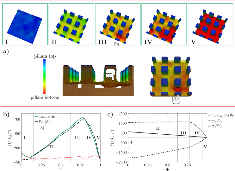
Figure 2: a) Collapse mechanism of the superhydrophobic Cassie state, shown by the density isosurface $\rho^{\ast}=0.5\,\rho_{l}$, where $\rho_{l}$ is the bulk liquid density at the simulated pressure. Images I–V illustrate typical interface shapes corresponding to the different regimes discussed in the text. Black isolines identify the region where the liquid is in contact with the bottom wall (III–IV); color code indicates the meniscus elevation over the pillars bottom; the hand symbol identifies the liquid finger. The bottom images show the meniscus shape at the transition state, where a liquid finger is formed. b) Free energy profile as a function of the filling fraction at $\Delta P=0.011\,\varepsilon\sigma^{-3}$ as computed via the string method in collective variables (green) and via the macroscopic theory in Eq. (6) (black). The absolute value of the deviation between the two estimates is shown in red dotted line. c) Continuum analysis of the atomistic results based on Eq. (6): the solid-vapor, liquid-vapor, and volume contributions to the free energy are shown in dashed, dot-dashed, and solid lines, respectively. The volume of vapor is related to the vapor filling via $V_{v}=\Phi(N_{C}-N_{W})/(\rho_{l}-\rho_{v})$.

The Cassie-Wenzel transition can take place following different wetting paths; here we analyze the one having the highest probability. At the pressures and temperatures of interest for technological applications (e.g., drag reduction), the Cassie and Wenzel states are separated by large free energy barriers that the system has to overcome. Thus, even if thermodynamics might favor the collapse, the system still has to climb the free energy barrier separating the initial and final state. This apparently non spontaneous process can take place only thanks to thermal fluctuations Bonella et al. (2012); Lelièvre et al. (2010). This implies infrequent transition events or, which is equivalent, long transition times, much longer than the typical timescale accessible to brute force (standard) MD. Thus, here the most probable wetting path is computed using a special technique – the string method in collective variables Maragliano et al. (2006), which is described in detail in Sec. II. It is important to remark that in the string method the pressure and temperature are kept constant at the prescribed values; in other words, the path obtained via the string method is representative of the transition at constant pressure and temperature.

The path is constituted by a sequence of atomistic coarse-grained density fields $\rho(\bm{x})$ (Eq. (1)), i.e., the path can be seen as a series of snapshots of the density field taken at different times along the transition from the Cassie to the Wenzel state. It is important to remark that each $\rho(\bm{x})$ is obtained by performing the ensemble average over atomistic configurations consistent with the state of the system along the path; thus, $\rho(\bm{x})$ contains all the nanoscale information. The morphology of the interface between the liquid and the vapor domains, the meniscus, is a simpler and more visual observable to follow the collapse mechanism. Thus, in the following the meniscus, which can be computed from $\rho(\bm{x})$, will be used to describe the change of morphologies of the liquid along the collapse process, and its effect on the free energy. These morphologies will be discussed in detail, with particular attention to clarify the role of nanoscale aspects such as line tension.

Figure 2 shows the collapse mechanism of the superhydrophobic state and the related free energy profile $\Omega(\Phi)$ along the most probable wetting path at a pressure and temperature close to the Cassie-Wenzel coexistence (i.e., where the Cassie and Wenzel states have approximatively the same free energy, $T=0.8\,\varepsilon k_{B}^{-1}$ and $\Delta P=0.011\,\varepsilon\sigma^{-3}$). $\Phi$ denotes the filling fraction defined as $\Phi\equiv(N-N_{C})/(N_{W}-N_{C})$, with $N$ the total number of liquid particles in the yellow regions of Fig. 1b and $N_{C}$ and $N_{W}$ the number of particles in the Cassie and Wenzel states, respectively. Here and in the following, notations of the type $\Omega(\Phi)$ are used as a shorthand for the more complete notation $\Omega\left(\rho({\bm{x}};\Phi)\right)$. The wetting path is divided into five parts (I–V), corresponding to different regimes.

In I, the meniscus is pinned at the top corners of the pillars, with its curvature increasing with $\Phi$. The free energy minimum corresponds to the Cassie state characterized by an almost flat meniscus as expected at low $\Delta P$.

In II, the meniscus depins from the corners and progressively slides along the pillars filling the interpillar space. The liquid-vapor interface has a small curvature which is sufficient to meet the pillars with the Young contact angle. Configurations in II correspond to a linear increase of the free energy. Given the large ratio between the height of the pillars and the spacing among them, the “sag” mechanism Patankar (2010); De Coninck et al. (2011), in which it is assumed that the meniscus remains pinned at the pillars corner along the entire process, cannot be realized.

The transition state (TS, free energy maximum) is found in III and corresponds to the liquid touching the bottom wall. In this part of the transition, the shape of the liquid-vapor interface changes dramatically: starting from an almost flat interface a liquid finger forms between two pillars and then touches the bottom wall (see Fig. 2a and ). The free energy barrier for collapse is very high for the considered pressure $\Delta P=0.011\,\varepsilon\sigma^{-3}$, $\Delta\Omega^{\dagger}_{CW}=670\;k_{B}T$. From this contact point, the liquid progressively fills the surrounding interpillar spaces. In the regions in which the liquid touches the bottom, the double liquid-vapor/vapor-solid interface is replaced by the liquid-solid interface, causing the free energy to decrease. It is clear that identifying correctly the most probable TS is especially important because this configuration determines the free energy barrier and, with exponential sensitivity, the collapse kinetics. In Sec. III.3 a comparison with other mechanisms proposed in the literature Patankar (2010); Prakash et al. (2016) shows how seemingly small morphological changes are reflected in radically different estimates of these quantities.

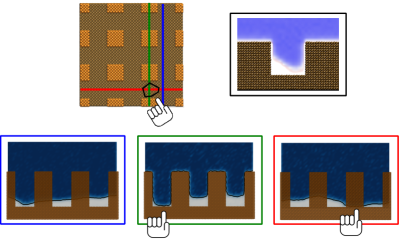
Figure 3: Two-dimensional cuts of the number density at the transition state: the liquid finger (identified by the hand symbol) forms at the intersection of the red and green planes. Bulk liquid density is represented in blue and vapor in white; black isolines identify the liquid-vapor interface. The density field at the top right is taken from the string simulations of Ref. Giacomello et al. (2015), where a quasi-2D groove is considered.

A closer look to the configurations around the TS shows that the finger formation involves both quasi-2D and collective wetting of the pillars (Fig. 3). In one direction (green line in Fig. 3), the liquid finger is strongly confined between pillars. Confinement renders the wetting mechanism effectively 2D close to the pillars centers, as demonstrated by comparing the second cut of the density field in Fig. 3 with the 2D mechanisms of previous works Giacomello et al. (2015): the wetting of the bottom wall happens via the formation of two asymmetric bubbles at the pillars lower corners with the smaller bubble disappearing faster. In the orthogonal direction (red line in Fig. 3) and far from the confined finger (blue line) the liquid-vapor interface must bend in order to recover the flat shape; the ensuing curvature of the interface is gentle because of surface tension. This collective, large scale mechanism triggers the wetting of the interpillar spaces surrounding the initial finger, causing the final collapse of the vapor domain.

Figures 2a and 3 show that the collapse is asymmetric and involves many interpillars spacings; this fact suggests that assuming a symmetric mechanism Patankar (2010) or simulating a single elementary cell is insufficient to capture correctly the mechanism and the related free energy since it imposes an unphysical symmetry to the problem. Even for the large domain simulated here, the effect of periodic boundary conditions becomes apparent at large filling levels beyond the TS; this however does not affect the estimation of the free energy barriers.

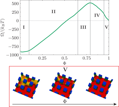
Figure 4: Top) Free energy profile at bulk liquid-vapor coexistence, $\Delta P\approx 0$ computed via the atomistic string. Bottom) Formation of density-depleted regions in between the pillars in part V of the collapse and percolation thereof. Same color code as in Fig. 2.

The present simulations can also help understanding the mechanism of the opposite process, i.e., the dewetting transition from Wenzel to Cassie. Indeed, under the hypothesis of a quasi-static transformation implicit in the string method, the forward and backward processes happen reversibly along the same path . Thus, here we describe the Wenzel-Cassie process associated to the path in Fig. 2 paying particular attention to the aspects relevant to dewetting. In order to do that in Fig. 4 we report the free energy profile at conditions close to bulk liquid vapor coexistence, $\Delta P\approx 0$. Dewetting, corresponding to the nucleation of a vapor domain in the textured surface, starts with the formation of two low-density, flat domains at the bottom of two facing pillars. These domains grow and merge, forming a single depleted region in between the pillars. This domain then percolates to the neighboring pillars, forming a connected network. While the string identifies only one percolating network, the texture geometry suggests that many such networks are possible, all of which involve multiple pillars. It must be stressed that this initial “collective” nucleation process, which corresponds to part V of Fig. 2, cannot be captured by simulating a single pillar or an elementary cell in one or two directions Prakash et al. (2016); Panter and Kusumaatmaja (2017); Savoy and Escobedo (2012a, b). Further moving toward the Cassie state, the percolating, depleted domain starts to form also in the spaces among four pillars, and detaches from the bottom forming a proper bubble. This part of the path corresponds to domain IV, where the free energy shows a descending trend with different slope. This branch of the process is completed when the liquid finger finally detaches from the bottom of the surface in a point in between two pillars, domain III. The free energy barrier for dewetting at $\Delta P\approx 0$ is $480\;k_{B}T$.

III.2 A sharp-interface interpretation of the atomistic mechanism

In order to rationalize the atomistic results in simple energetic terms, a macroscopic, sharp-interface model of capillarity is used in connection with the data summarized in Fig. 2. For this model the free energy reads Kelton and Greer (2010):

$$\Omega_{\mathrm{macro}}\equiv\Omega-\Omega_{\mathrm{ref}}=\Delta PV_{v}+\gamma_{lv}\left(A_{lv}+\cos\theta_{Y}A_{sv}\right)\text{ ,}$$ (6)

where the Wenzel free energy $\Omega_{\mathrm{ref}}=\Delta PV_{\mathrm{tot}}-\gamma_{lv}\cos\theta_{Y}A_{\mathrm{tot}}$ is taken as a reference and $V_{\mathrm{tot}}$ and $A_{\mathrm{tot}}$ are the total volume of the interpillar space and its internal surface area, respectively. It is important to remark that $\Omega_{\mathrm{macro}}$ actually depends on the shape of the liquid-vapor interface $\Sigma_{lv}$, which, in turn, determines the solid-vapor one $\Sigma_{sv}$ and the vapor volume $V_{v}$. Since $\Omega_{\mathrm{macro}}$ defined in Eq. (6) is a functional of the complete $\Sigma_{lv}$, it can be computed for arbitrarily complex configurations of the capillary system, e.g., along wetting paths which may or may not contain collective effects. The first term on the RHS corresponds to the bulk energy of a system containing a vapor bubble of volume $V_{v}$: at $\Delta P>0$ vapor bubbles are energetically hindered while at negative pressures they are favored. This term is the driving force for the liquid-vapor transition. The second terms on the RHS are the energy cost of the liquid-vapor and solid-vapor interfaces, respectively; both are multiplied by the liquid-vapor surface tension $\gamma_{lv}$. The cost of $A_{sv}$ is modulated by the Young contact angle $\cos\theta_{Y}\equiv(\gamma_{sv}-\gamma_{sl})/\gamma_{lv}$. In the hydrophobic case considered here ($\theta_{Y}>\pi/2$), it is energetically favorable to increase $A_{sv}$, e.g., by dewetting the pillars: this is why at the liquid-vapor bulk coexistence ($\Delta P\approx 0$) the Cassie state is thermodynamically stable.

The terms in Eq. (6), which are needed in order to make a connection with the atomistic simulations, are consistent with the properties of the atomistic system and can be computed as follows (see Supplemental Material for details on the calculations of the contact angle, surface tension, and areas Note (2)). $\Delta P=0.011\,\varepsilon\sigma^{-3}$ is controlled by the barostat, while $\gamma_{lv}=0.57\,\varepsilon\sigma^{-2}$ and $\theta_{Y}=113^{\circ}$ are computed via independent MD simulations. The liquid-vapor and solid-liquid areas are computed by applying the marching cube method Lorensen and Cline (1987) on the $1\times 1\times 1\,\sigma^{3}$ coarse-grained density field obtained from the string calculations. The volume of vapor is computed as $V_{v}\equiv(N_{W}-N)/(\rho_{l}-\rho_{v})$, where $N_{W}$ and $N$ are the number of particles within the yellow region of Fig. 1 in the Wenzel and in a generic state, respectively, and $\rho_{l}$ and $\rho_{v}$ are the bulk liquid and vapor densities. It is important to remark that all the physical quantities are computed independently, i.e., they are not fitted to reproduce the atomistic free energy profile of wetting.

Figure 2b shows a fair agreement between the atomistic free energy and Eq. (6). In particular, the model in Eq. (6) does not include line tension, which is often invoked to explain in macroscopic terms nanoscale wetting phenomena Sharma and Debenedetti (2012); Guillemot et al. (2012). One notices that the energetic difference between the atomistic and macroscopic models (dotted red curve of Fig. 2b) is a small fraction of the wetting barrier, $\approx 10~{}\%$. This suggest that nanoscale effects, which include line tension, dependence of the surface tension on the curvature of the meniscus, width of the interfaces, etc., play a minor role in the transition path and kinetics of the wetting. In particular, considering that the contact line changes significantly in the regimes III-V, the present results indicate that line tension does not change dramatically the free energy profile for hydrophobic pillars on the $3$ nm scale, pushing further down the limit where line effects might be relevant (recent experimental work on superhydrophobicity Checco et al. (2014) showed the same for textures down to $10$ nm). More precisely, the combination of atomistic simulations with the continuum analysis entailed in Eq. (6) shows that the contribution of line tension to the intrusion or nucleation free energy barriers is negligible for the present system. It will be interesting to use a similar approach to explore extreme confinement (of the order of a nanometer or less), where a major contribution of line tension is expected Sharma and Debenedetti (2012). The differences observed in the pinning region might be ascribed to the increased thickness of the liquid-vapor interface. In terms of macroscopic theories, the latter are associated to finite temperature effects, such as capillary waves. These effects, neglected in Eq. (6), are sizable at depinning and seem to make the sharp-interface model less reliable there.

Apart from these minor limitations, Eq. (6) provides a simple interpretation of the atomistic collapse mechanism shown in Fig. 2a. In I, the area of the liquid-vapor interface $A_{lv}$ slightly increases, reflecting the increasing curvature due to pinning. At the same time the top surface and corners of the pillars become wet and the area of the solid-vapor interface $A_{sv}$ decreases.

In II, $A_{lv}$ remains constant, while $A_{sv}$ linearly decreases, which corresponds to an increase of the interface area between the liquid and the hydrophobic solid. This surface term more than balances the decreasing bulk term $\Delta PV_{v}$, resulting into a linear increase of the free energy. If the interface were to keep this “flat” configuration until the bottom surface is fully wet, as assumed in classical works Patankar (2003, 2010), the linear trend would continue, determining a much larger free energy barrier $\Delta\Omega_{CW}^{\dagger}=920\;k_{B}T$. This figure would lead, in turn, to estimate a lifetime of superhydrophobicity exponentially longer than for the mechanism shown in Fig. 2 ($10^{108}$ times). Instead, at variance with the classical mechanism, at a distance $h_{TS}\approx 6\,\sigma$ from the bottom surface (part III), it is energetically more convenient to bend the liquid-vapor interface between two pillars. The free energy of formation of this finger is seen to be negligible, while it allows the liquid to wet the bottom surface. Thus, the two liquid-vapor and vapor-solid interfaces are replaced by a single liquid-solid one, which decreases the total free energy by $\Omega_{\mathrm{dry}}-\Omega_{\mathrm{wet}}=\gamma_{lv}(A_{\mathrm{lv,dry}}+\cos\theta_{Y}A_{\mathrm{sv,dry}})>0$ (Fig. 2c).

III.3 Comparison with results in the literature

It is now possible to compare the path in Fig. 2 obtained via the atomistic string with those available in the literature and computed via continuum Ren (2014); Pashos et al. (2016) and atomistic Savoy and Escobedo (2012a); Prakash et al. (2016) simulations. Pashos et al. Pashos et al. (2016) considered a sharp interface model for the liquid-vapor interface with an empirical diffuse liquid-solid potential, which was introduced in order to simplify the numerical treatment of complex textures and topological changes of the meniscus (for a similar approach, see Ref. Giacomello et al. (2015) – see also Supplemental Material for the effective diffuse liquid-solid potential computed via MD for the present solid-liquid interactions Note (2)). The pillar height-to-width ratio is very low, such that the surface is physically reminiscent of a naturally rough one rather than the artificial textures used for superhydrophobicity Checco et al. (2014). In particular, the interaction length of the liquid-solid potential is roughly half the pillar height. The path obtained with this model is still characterized by the formation of a liquid finger touching the bottom wall in a single point with the liquid front then moving to neighboring pillars. However, the free energy profile is very different from the present, with a number of intermediate transition states. This discrepancy is not unexpected, given the different pillars height and the different range of potentials employed.

Ren and coworkers Ren (2014); Zhang and Ren (2014) combined the string method with a mesoscale diffuse interface model in order to study the impalement of a drop on 3D surfaces with (slender) pillars. Although the system is rather different from the present one, the finger mechanism was found to be always energetically favorable. The finite lateral extent of the drop, however, significantly alters the advanced phase of the Cassie-Wenzel transition.

Savoy and Escobedo Savoy and Escobedo (2012a) studied the Cassie-Wenzel transition of a nanodroplet on quasi-2D pillars. In their atomistic trajectories obtained via forward flux sampling (FFS) Allen et al. (2009) the formation of a liquid finger can also be identified in some atomistic configurations. However it is difficult to compare other details of the path and the energetics, because the FFS method only gives access to independent atomistic trajectories and not to the most probable density field as for the string.

Patel and coworkers Prakash et al. (2016) used umbrella sampling to study the collapse of the submerged superhydrophobic state on pillars. This geometry is very close to the present one, the main difference being that there a single elementary cell was studied, which, due to the periodic boundary conditions, corresponds to the wetting of a single pillar. While a sort of finger formation is observed in correspondence of the transition state, the subsequent wetting process substantially differs from that in Fig. 2 in two respects. The first one is that the wetting process is discontinuous, with jumps in the density field between neighboring configurations. This is a known artifact ensuing from the use of a single collective variable Giacomello et al. (2015) that cannot distinguish among bubble shapes enclosing the same volume $V_{v}$; a detailed analysis on the choice of the CVs will be object of an upcoming work. The second difference is the shape of the vapor bubbles during the later stage of the transition: the use of a single elementary cell imposes a symmetry to them which does not necessarily correspond to the most probable one.

Summarizing this analysis of available simulations, the formation of a liquid finger has been reported in a number of previous works dealing with both drops and submerged surfaces, tall and short posts Dupuis and Yeomans (2005); Kusumaatmaja and Yeomans (2007); Savoy and Escobedo (2012a); Ren (2014); Pashos et al. (2016); Prakash et al. (2016); Panter and Kusumaatmaja (2017). There are, however, also relevant differences in the configuration of this transition state. Here, the liquid finger forms between two pillars; in such a way the liquid-vapor interface bends only on two sides of the pillars, while the remaining sides become wet. This is energetically favorable because the cost of replacing a portion of the two liquid-vapor and solid-vapor interfaces with a solid-liquid interface is lower than that of increasing $A_{lv}$, $-\gamma_{lv}\cos\theta_{Y}<\gamma_{lv}$. Therefore it seems that the exact point where the finger forms and, consequently, where the transition state occurs, depends on the details of the confining geometry (in particular on the height/spacing ratio of the pillars) and on the chemistry of the surface.

In general terms, the presence of the bottom surface breaks the translational symmetry of the meniscus sliding along the pillars and thus imposes a change of topology to the vapor bubble. The local formation of a single, relatively narrow liquid finger is the energetically favored way to accomplish this transition. It is still an open question whether the finger should touch the bottom surface symmetrically or not, i.e., if two equivalent vapor bubbles are formed at the bottom of the two pillars confining the finger. For the 2D groove geometry, simulations have suggested that the asymmetric pathway is energetically favored because it allows the formation of a single vapor bubble in a corner Giacomello et al. (2012b, 2015). However, this finding does not exclude that other pathways are possible and might also be favored for other reasons (e.g., kinetic/inertia reasons). Indeed recent experiments Lv et al. (2015) on a similar geometry suggest that both pathways are possible. Moreover, recent string calculations Panter and Kusumaatmaja (2017) underscore that in 2D grooves pathways with both symmetric and asymmetric bubbles are possible, with the latter having a slightly lower free energy barrier.

On pillared surfaces, careful analysis of the collapse of the superhydrophobic state by confocal microscopy Papadopoulos et al. (2013) revealed the (abrupt) formation of vapor bubbles at one of the pillars’ lower corners, after the first contact with the bottom wall. This asymmetry in the last stage of the wetting process possibly indicates that the finger formation, which is too fast to be experimentally observed, was asymmetric too.

IV Conclusions

In summary, rare-event atomistic simulations have provided a detailed description of the collapse of the superhydrophobic Cassie state on a nanopillared surface. This system is often encountered in experiments and serves as a prototype for wetting of interconnected cavities. Results have showed that the collapse proceeds in five stages: depinning of the liquid-vapor interface from the pillars’ corners; progressive wetting of the pillars via an almost flat, horizontal meniscus; formation of a liquid finger between two pillars which touches the bottom wall; progressive filling by a non-flat meniscus; absorption of a percolating network of low-density domains connecting pairs of pillars. This mechanism is very different from 2D grooves Patankar (2003); De Coninck et al. (2011); Giacomello et al. (2015) and also from other 3D simulations Prakash et al. (2016) and could be captured only with state-of-the-art simulation techniques. On one hand, results indicate that the system should be large enough to capture the local formation of a liquid finger and the progressive filling of the surrounding spaces. On the other hand, the number and choice of collective variables should allow one to resolve density changes in between the pillars. These caveats should be born in mind for simulations of wetting: artifacts can conceal the actual collapse mechanism, affect the estimation of the free energy barriers and, with exponential sensitivity, of the collapse kinetics. The continuum analysis of the MD results entailed in Eq. (6) has allowed us to identify the different area and volume contributions to the free energy along the collapse, showing that line tension, evaporation/condensation, and other nanoscale effects are negligible in the present conditions. These results shed new light on the wetting process of interconnected gas reservoirs which can open new perspectives in the design of nanotextures.

Appendix A Appendix: the string method in collective variables

Referring to the specialized literature for a complete derivation Maragliano et al. (2006), a brief summary of the steps needed to obtain Eq. (2) is given below to provide the uninitiated reader with the basic conceptual framework of the string method in collective variables:

• A system of stochastic differential equations in the phase space of the original microscopic system (the $6n_{f}$-dimensional space given by the vector of coordinates $\bm{r}$ and velocities –momenta expressed in mass reduced coordinates– ${\bm{v}}={\dot{\bm{r}}}$) is devised whose statistically steady solution follow the equilibrium probability distribution $m({\bm{r}},{\bm{v}})$ specified by the given ensemble Maragliano et al. (2006). Its configurational part is the distribution $m({\bm{r}})=\int\mathrm{d}{\bm{v}}\;m({\bm{r}},{\bm{v}})$ in Eq.. (3) and (4).

• The backward Kolmogorov equation (BKE) $Lq=0$ associated with the system of stochastic differential equations is identified. BKE is a partial differential equation for the scalar quantity $q$ in the $6n_{f}$-dimensional phase space of the system. $L$ is a linear partial differential operator involving derivatives with respect to both $\bm{r}$ and $\bm{v}$, $L=L_{{\bm{r}},{\bm{v}}}$. When BKE is solved with boundary conditions $q\left({\bm{r}},{\bm{v}}\right)=0$ for $\left({\bm{r}},{\bm{v}}\right)\in A$ and $q\left({\bm{r}},{\bm{v}}\right)=1$ for $\left({\bm{r}},{\bm{v}}\right)\in B$, where $A$ and $B$ are the two sets in phase space corresponding to the two metastable macroscopic states (Cassie and Wenzel, respectively) to be addressed, its solution provides the committor $q\left({\bm{r}},{\bm{v}}\right)$. $q$ gives the probability that the state $\left({\bm{r}},{\bm{v}}\right)$ will reach $B$ (the products, in the chemical nomenclature) before reaching $A$ (the reactants). The solution of the BKE satisfies a minimum principle for the functional $I=\int m\left({\bm{r}},{\bm{v}}\right)|Lq|^{2}d{\bm{r}}d{\bm{v}}$ under the given boundary conditions. The committor is the actual reaction coordinate of the transition from $A$ to $B$, and its level surfaces $q\left({\bm{r}},{\bm{v}}\right)=q_{0}$ are the loci of the micro-states with the same progress of the reaction.

• It is assumed that the selected collective variable, namely the coarse-grained density field $\theta({\bm{r}},{\bm{x}})$, provides a good description of the transition. As a consequence the transition is described as well by minimizing the restriction $\tilde{I}$ of $I$ to the space of functions $f(\rho_{1},\ldots,\rho_{M})$ defined on the coarse grained density field. This is tantamount to assuming $q\simeq f\left[\theta({\bm{r}},{\bm{x}})\right]$. Two aspects are worth being noted: a) the minimum of $\tilde{I}$ is now searched in the space of functions of $M$ variables, $f(\rho_{1},\ldots,\rho_{M})$, rather than in that of functions $q$ defined on the $6n_{f}$-dimensional phase space. b) The CVs are taken to depend only on the configuration of the particles and not on their velocities ${\bm{v}}$. As we shall immediately see, upon minimizing $\tilde{I}$ with respect to $\theta$, certain averages naturally emerge. The functional

  $$\tilde{I}=\int\mathrm{d}{\bm{r}}\mathrm{d}{\bm{v}}\;m\left({\bm{r}},{\bm{v}}\right)Lf\left[\theta\left({\bm{r}},{\bm{x}}\right)\right]L\,f\left[\theta\left({\bm{r}},{\bm{x}}\right)\right]=$$

  $$\int d{\bm{v}}\;m_{\bm{v}}\left({\bm{v}}\right)\int\mathrm{d}{\bm{r}}\;m_{\bm{r}}\left({\bm{r}}\right)L_{{\bm{r}}}f\left[\theta\left({\bm{r}},{\bm{x}}\right)\right]L_{{\bm{r}}}f\left[\theta\left({\bm{r}},{\bm{x}}\right)\right]\,,$$

  where the pdf of the relevant ensemble is typically factorized, $m\left({\bm{r}},{\bm{v}}\right)=m_{\bm{v}}\left({\bm{v}}\right)m_{\bm{r}}\left({\bm{r}}\right)$, and $L_{\bm{r}}$ is the part of $L_{{\bm{r}},{\bm{v}}}$, only involves derivatives with respect to the configuration $\bm{r}$. To proceed further, the explicit expression of $L_{\bm{r}}$ is needed. For the system we are considering it turns out to be $L_{\bm{r}}={\bm{v}}_{i}\cdot\partial/\partial{{\bm{r}}_{i}}$ (sum is implied on repeated indices).

  It follows

  $$\tilde{I}= \int\mathrm{d}{\bm{v}}\;m_{\bm{v}}\left({\bm{v}}\right){\bm{v}}_{p}\otimes{\bm{v}}_{l}:\int\mathrm{d}{\bm{r}}\;m_{\bm{r}}\left({\bm{r}}\right)\frac{\partial f}{\partial\theta_{i}}\frac{\partial\theta_{i}}{\partial{\bm{r}}_{p}}\otimes\frac{\partial\theta_{j}}{\partial{\bm{r}}_{l}}\frac{\partial f}{\partial\theta_{j}}=$$

  $$C\int\mathrm{d}{\bm{r}}\;m_{\bm{r}}\left({\bm{r}}\right)\frac{\partial f}{\partial\theta_{i}}\frac{\partial\theta_{i}}{\partial{\bm{r}}_{p}}\cdot\frac{\partial\theta_{j}}{\partial{\bm{r}}_{p}}\frac{\partial f}{\partial\theta_{j}}=$$

  $$C\int\mathrm{d}{\bm{r}}\;m_{\bm{r}}\left({\bm{r}}\right)\frac{\partial\theta_{i}}{\partial{\bm{r}}_{p}}\cdot\frac{\partial\theta_{j}}{\partial{\bm{r}}_{p}}\int\mathrm{d}\rho_{1}\ldots\mathrm{d}\rho_{M}\;\frac{\partial f}{\partial\rho_{i}}\frac{\partial f}{\partial\rho_{j}}$$

  $$\quad\qquad\qquad\qquad\qquad\delta\left[\rho_{1}-\theta_{1}({\bm{r}}) \right]\ldots\delta\left[\rho_{M}-\theta_{M}({\bm{r}}) \right]=$$

  $$C\int\mathrm{d}\rho_{1}\ldots\mathrm{d}\rho_{M}\;\mathrm{e}^{-\beta\Omega(\rho_{1},\ldots,\rho_{M})}\frac{\partial f}{\partial\rho_{i}}\frac{\partial f}{\partial\rho_{j}}$$

  $$\quad\quad\frac{\displaystyle\int\mathrm{d}{\bm{r}}\;m_{\bm{r}}\left({\bm{r}}\right)\frac{\partial\theta_{i}}{\partial{\bm{r}}_{p}}\cdot\frac{\partial\theta_{j}}{\partial{\bm{r}}_{p}}\delta\left[\rho_{1}-\theta_{1}({\bm{r}}) \right]\ldots\delta\left[\rho_{M}-\theta_{M}({\bm{r}}) \right]}{\displaystyle\int\mathrm{d}{\bm{r}}\;m_{\bm{r}}\left({\bm{r}}\right)\delta\left[\rho_{1}-\theta_{1}({\bm{r}}) \right]\ldots\delta\left[\rho_{M}-\theta_{M}({\bm{r}}) \right]}=$$

  $$C\int\mathrm{d}\rho_{1}\ldots\rho_{m}\;\mathrm{e}^{-\beta\Omega(\rho_{1},\ldots,\rho_{M})}\frac{\partial f}{\partial\rho_{i}}\frac{\partial f}{\partial\rho_{j}}g_{ij}\left(\rho_{1},\ldots,\rho_{M}\right)\,,$$

  where $\Omega\left(\rho_{1},\ldots,\rho_{M}\right)$ and $g_{ij}\left(\rho_{1},\ldots,\rho_{M}\right)$ have been defined in Eq.. (3) and (4), respectively. Note that $\int\mathrm{d}\bm{v}\;m_{\bm{v}}(\bm{v}){\bm{v}}_{p}\otimes{\bm{v}}_{l}=C\delta_{pl}$ since the velocity of particle $p$ is independent from particle $l$.

• The Euler-Lagrange equations for the restricted functional $\tilde{I}$ are easily derived as

  $$\frac{\partial}{\partial\rho_{i}}\left(\mathrm{e}^{-\beta\Omega\left(\rho_{1},\ldots,\rho_{M}\right)}g_{ij}\frac{\partial f}{\partial\rho_{j}}\right)=0\,,$$

  and can be interpreted as the backward Kolmogorov equation of the stochastic differential equation

  $$\frac{\mathrm{d}\rho_{i}}{\mathrm{d}\tau}=-g_{ij}\frac{\partial\Omega}{\partial\rho_{j}}-\frac{1}{\beta}\frac{\partial g_{ij}}{\partial\rho_{j}}+\sqrt{\frac{2}{\beta}}g_{ij}^{1/2}\xi_{j}\,,$$

  where $\xi_{s}$ is a white noise, $\langle\xi_{s}\rangle=0$, $\langle\xi_{s}(\tau)\xi_{r}(\tau^{\prime})\rangle=\delta_{sr}\delta\left(\tau-\tau^{\prime}\right)$.

• When the thermal energy $1/\beta=k_{B}T$ is small with respect to the typical free energy variation along the path (of the order of the free energy barrier the system has to overcome to undergo the transition which, for rare events, is always much larger than $k_{B}T$) the leading term in $k_{B}T$ is negligible and one is left with a stochastic dynamics in which the probability of a discrete path connecting the initial and final state is a product of Gaussian terms. One can, thus, search for the most probable among these paths, i.e., the path that the transition almost certainly follows:

  $$\frac{\mathrm{d}\rho_{i}}{\mathrm{d}\tau}=-g_{ij}\frac{\partial\Omega}{\partial\rho_{j}}\,,$$

  with boundary conditions $\rho_{a}\in a$ and $\rho_{b}\in b$, being $a$ and $b$ the two sets in the space of coarse grained density distributions which corresponds to the Cassie and the Wenzel state, respectively. The problem, as stated in the main text, cannot be easily solved by direct integration. Reparametrization of the curve $\rho({\bm{x}})$ in terms of the arc-length $\lambda$ yields Eq. (2) and the problem can be reinterpreted as the relaxation of a string $\rho\left(\bm{x};\lambda\right)$ joining the two metastable states $\rho({\bm{x}},0)=\rho_{a}\in a$ and $\rho({\bm{x}},1)=\rho_{b}\in b$ towards the most probable path.