Radiative decays $\chi_{cJ}\rightarrow V\gamma$ within the QCD factorisation framework

Abstract

We present a discussion of radiative decays $\chi_{cJ}\rightarrow\gamma\rho(\omega,\phi)$. The decay amplitudes are computed within the QCD factorisation framework. NRQCD has been used in the heavy meson sector as well as a collinear expansion in order to describe the overlap with light mesons in the final state. The colour-singlet contributions to all helicity amplitudes have been computed using the light-cone distribution amplitudes of twist-2 and twist-3. All obtained expressions are well defined at least in the leading-order approximation. The colour-octet contributions have also been studied in the Coulomb limit in order to exhibit their scaling behaviour. In order to understand the relevance of the different contributions we perform numerical estimates using the colour-singlet contributions. For the $\chi_{c1}\rightarrow\gamma V_{\perp}$ decays, to vector mesons with transverse polarisation, we find that the colour-singlet contribution potentially allows for a reliable description. On the other hand, for the $\chi_{c1}\rightarrow\gamma V_{\|}$ decays, to vector mesons with longitudinal polarisation, our findings indicate that the colour-octet mechanism may be important for a good description. We expect that more accurate measurements of the decay $\chi_{c2}\rightarrow\gamma V_{\perp,\|}$ can help to better understand the mechanism of radiative decays.

1 Introduction

The radiative decays of $P$-wave charmonia $\chi_{cJ}$ have been measured by different experimental collaborations: CLEO [1] and BESIII [2]. Theoretical estimates have been given in Refs.[3, 4]. In these papers, the authors use the pQCD formalism in combination with specific models for the light meson wave functions, and the constituent quark masses have been used as infrared regulator in these calculations. The obtained estimates for the $\chi_{c1}\rightarrow\rho(\omega,\phi)\gamma$ decay rates are few times smaller than the measured ones. To resolve this discrepancy the authors of Ref.[5] used a phenomenological model with intermediate $D-$meson interactions.

In Table 1 we collect the current branching fraction measurements for the decays which have been measured. From this table it is seen that the largest branchings for all channels are provided by decay $\chi_{c1}\rightarrow V\gamma$. Moreover, in this case the decay rate is dominated by the longitudinal meson ($V_{\|}$) in the final state.

	$\chi_{c1}\rightarrow V\gamma$	$\chi_{c1}\rightarrow V_{\|}\gamma$	$\chi_{c1}\rightarrow V_{\bot}\gamma$	$\chi_{c0}\rightarrow V\gamma$	$\chi_{c2}\rightarrow V\gamma$
$\gamma\rho$	$220\pm 18$	$184.8\pm 15.7$	$35.2\pm 7.4$	$<9$	$<20$
$\gamma\omega$	$69\pm 8$	$51.8\pm 8.9$	$17.3\pm 6.5$	$<8$	$<6$
$\gamma\phi$	$25\pm 5$	$17.7\pm 4.9$	$7.3\pm 3.6$	$<6$	$<8$

Table 1: The branching fractions $\chi_{cJ}\rightarrow V\gamma$ in units of $10^{-6}$. The total fractions are taken from the Review of Particle Physics [6]. The original experimental results can be found in [1, 2]. In order to obtain the different contributions for the $\chi_{c1}$ decays we used the ratios $f_{\bot}^{V}={\Gamma[\chi_{c1}\rightarrow V_{\bot}\gamma]}/{\Gamma[\chi_{c1}\rightarrow V\gamma]}$ from Ref.[2].

The data presented in Refs.[1, 2] also allow one to study the contributions of the different helicity amplitudes which can provide additional interesting information about the underlying mechanism of quark-gluon interactions. This point has not yet been considered to full extent in the literature. For instance, within the systematic QCD factorisation framework the leading-order contribution with a longitudinal outgoing vector meson is given by the diagram as in Fig.1$(a)$ but for a transversely polarised meson ($V_{\perp}$) one has to consider the matrix element with the three particle wave functions as in Fig.1$(b)$ and Fig.1$(c)$. The first diagram is of order $\alpha_{s}^{2}$, the second is of order $\alpha_{s}$ but suppressed by a factor $\Lambda_{QCD}/m_{c}$ because of subleading twist-3 collinear operators describing the overlap with the light outgoing meson.

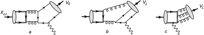
Figure 1: The various contributions to the decay amplitudes: $(a)$ the leading-order contribution for the longitudinal amplitude with $V_{\|}$; $(b)$ and $(c)$ two different contributions for the transverse amplitude with $V_{\perp}$.

A description of the reactions with charmonium states can be challenging because of possible large contributions of the colour-octet operators; see, e.g., review [7] and references therein. This mechanism could be especially important for the description of exclusive $P$-wave hadronic decays and has been studied within a phenomenological framework in Refs.[8, 9] and in the Coulomb limit in Ref.[10]. The contributions with the colour-octet operators can also play an important role in the description of the radiative decays of $\chi_{cJ}$. A hint about this can be seen from the following observation.

The various contributions to the decay amplitudes can be associated with the following two matrix elements: either the photon is emitted from the light quark or from the heavy quark

$$\langle V(p)|J^{\mu}_{em}|\chi_{cJ}\rangle=\langle V(p)|\sum_{u,d,s}e_{q}\ \bar{q}\gamma^{\mu}q|\chi_{cJ}\rangle+\langle V(p)|e_{c}\ \bar{c}\gamma^{\mu}c|\chi_{cJ}\rangle$$ (1)

If the dominant contribution to the decay amplitudes is provided by the light quark component of the electromagnetic current in Eq.(1) then using $SU(2)$ in the light quark sector one can establish the relations between the branching fractions for different vector mesons in the final state. For instance, one easily finds the relation ${Br\left[\chi_{c1}\rightarrow\omega\gamma\right]}/{Br\left[\chi_{c1}\rightarrow\rho\gamma\right]}\simeq\frac{1}{9}$ . This prediction can be easily understood if one assumes that the decay amplitude is dominated by the hard two-gluon intermediate state as in Fig. 1$a$. The same arguments must also be valid for the colour-octet contribution which originates from the light-quark matrix element in Eq.(1). However, as one can see from the data in Table 1, the given ratio is about a factor 3 larger than expected. This allows one to assume that the heavy quark matrix element in Eq.(1) also gives contributions with a sizable numerical impact. However in the factorisation framework the corresponding contribution with longitudinal mesons $V$ can only be associated with the colour-octet mechanism.

In order to better understand the relevance of the various contributions, in this work we compute the helicity amplitudes within the standard QCD factorisation framework and study the possible colour-octet contributions in the Coulomb limit. The factorisation approach is closely related with the effective theories inspired by QCD: NRQCD [11, 12, 13] for the heavy quark sector and the soft-collinear effective theory (SCET) [14, 15, 16, 17, 18, 19] for the collinear sector associated with the light mesons in the final state. The important advantage of this scheme is that it allows one to perform systematic expansions with respect to the small relative velocity $v$ and $\lambda^{2}\sim\Lambda_{QCD}/m_{Q}$. Hence one can classify various operators with respect to these parameters and this can guide us on the relevance of the different contributions.

The outline of this paper is as follows. In Sec. 2 we provide the basic notations and description of the decay amplitudes and decay width. Then we compute the contributions of the colour-singlet operators for different polarisations of the outgoing light meson. We show that the leading-order contributions are factorizable and establish their scaling behaviour. This behaviour can be qualitatively compared with the behaviour of the colour-octet contributions in the Coulomb limit. This allows us to make a qualitative conclusion about the importance of the colour-octet matrix elements. In Sec. 3 we perform numerical estimates of the branching fractions using only the colour-singlet approximations for the decay amplitudes. This analysis allows us to make some more realistic conclusions about possible mechanism of the radiative decays. The summary of our results is presented in Sec. 4. In Appendixes A and B we provide a description of the different vector meson distribution amplitudes and present technical details on the estimates of the colour-octet matrix elements in the Coulomb limit.

2 Colour-singlet contributions in the factorisation framework

2.1 Kinematics and amplitudes.

The amplitude of decay $\chi_{cJ}(P)\rightarrow\gamma(q)+V(p)$ is defined as

$$\left\langle\gamma(q)V(p);\text{out}\right|\left.\text{in};\chi_{cJ}(P)\right\rangle=i(2\pi)^{4}\delta(P-p-q)\ \mathcal{A}_{\chi_{cJ}\rightarrow V\gamma},$$ (2)

where

$$\ \mathcal{A}_{\chi_{cJ}\rightarrow V\gamma}=\left\langle V(p)\right|\epsilon_{\gamma}^{\ast}\cdot J_{em}(0)\left|\chi_{cJ}(P)\right\rangle,$$ (3)

with electromagnetic current

$$J_{em}^{\mu}(0)=\sum_{q=u,d,s,c}ee_{q}\bar{q}(0)\gamma^{\mu}q(0),$$ (4)

here $\epsilon_{\gamma}^{\ast}$ is the photon polarisation vector. In the following we use the frame where the heavy meson is at rest and the $z$-axis is chosen along the momenta of the outgoing particles

$$P=M_{J}(1,\vec{0})=M_{J}\omega,$$ (5)

where $M_{J}$ is the mass of the heavy quarkonia and $\omega$ denotes its four-velocity. The outgoing momenta read

$$q=E_{\gamma}(1,0,0,1)=2E_{\gamma}\frac{\bar{n}}{2},~{}\ p=(\sqrt{m_{V}^{2}+E_{\gamma}^{2}},0,0,-E_{\gamma}),~{}~{}E_{\gamma}=\frac{M_{J}^{2}-m_{V}^{2}}{2M_{J}}.$$ (6)

Using that the heavy quark mass is quite large $m\gg\Lambda_{QCD}$ one finds

$$~{}q\simeq m(1,0,0,1)=2m\frac{\bar{n}}{2},~{}\ \ p\simeq m(1,0,0,-1)=2m\frac{n}{2},$$ (7)

where we introduced auxiliary light-cone vectors $n$ and $\bar{n}$ with $(n\bar{n})=2$.  The four-velocity in Eq.(5) reads

$$\omega=\frac{1}{2}\left(n+\bar{n}\right),~{}\ \omega^{2}=1.$$ (8)

Any four-vector $F^{\mu}$ can be expanded as

$$F^{\mu}=\left(F\cdot n\right)\frac{\bar{n}^{\mu}}{2}+\left(F\cdot\bar{n}\right)\frac{n^{\mu}}{2}+F_{\bot}^{\mu},$$ (9)

where $F_{\bot}$ denotes the components transverse to the lightlike vectors : $\left(F_{\bot}\cdot n\right)=\left(F_{\bot}\cdot\bar{n}\right)=0$. Similarly, one can also write a decomposition

$$F^{\mu}=\left(F\cdot\omega\right)\omega^{\mu}+F_{\top}^{\mu},$$ (10)

where $F_{\top}$ denotes the component which is orthogonal to the velocity $\omega$: $\left(\omega\cdot F_{\top}\right)=0$.

The amplitudes defined in Eq.(3) can be parametrised as

$$\mathcal{A}_{\chi_{c0}\rightarrow V\gamma}=~{}\left(\epsilon_{V}^{\ast}\cdot\epsilon_{\gamma}^{\ast}\right)~{}M_{0}~{}A_{0V}^{\bot},$$ (11)

$$\mathcal{A}_{\chi_{c1}\rightarrow V\gamma}=~{}i\varepsilon[\epsilon_{\chi},\epsilon_{\gamma}^{\ast},p,q]~{}(\epsilon_{V}^{\ast}\cdot\omega)\frac{m_{V}}{M_{1}^{2}}~{}A_{1V}^{\|}+i\varepsilon[\epsilon_{V}^{\ast},\epsilon_{\gamma}^{\ast},p,q]~{}(\epsilon_{\chi}\cdot q)\frac{1}{M_{1}^{2}}~{}A_{1V}^{\bot},$$ (12)

$$\mathcal{A}_{\chi_{c2}\rightarrow V\gamma} =\epsilon_{\chi}^{\alpha\beta}q_{\alpha}\left(\epsilon_{\gamma}^{\ast}\right)_{\beta}(\epsilon_{V}^{\ast}\cdot\omega)~{}\frac{m_{V}}{M_{2}}~{}A_{2V}^{\|}+~{}\epsilon_{\chi}^{\alpha\beta}q_{\alpha}q_{\beta}\left(\epsilon_{V}^{\ast}\cdot\epsilon_{\gamma}^{\ast}\right)\frac{1}{M_{2}}~{}A_{2V}^{\bot}$$

$$+\epsilon_{\chi}^{\alpha\beta}\left\{(\epsilon_{\gamma}^{\ast})^{\alpha}(\epsilon_{V}^{\ast})^{\beta}+(\epsilon_{\gamma}^{\ast})^{\alpha}q^{\beta}(\epsilon_{V}^{\ast}\cdot q)\frac{(pP)}{(pq)^{2}}-q_{\alpha}q_{\beta}\left(\epsilon_{V}^{\ast}\cdot\epsilon_{\gamma}^{\ast}\right)\frac{1}{2E_{\gamma}^{2}}\right\}\frac{E_{\gamma}^{2}}{M_{2}}~{}T_{2V}^{\bot}.$$ (13)

where $\epsilon_{\chi}$ and $\epsilon_{V}^{\ast}$ denote polarisation vectors (or tensors in the case of $\chi_{c2}$) of the initial and final mesons, respectively. Furthermore, the amplitudes $A_{iV}^{\|}$ and $A_{iV}^{\bot}\ (T_{2V}^{\bot})$ correspond to the longitudinal and transverse vector meson $V$, respectively. In Eq.(12) the following notation has been used

$$i\varepsilon[\epsilon_{V}^{\ast},\epsilon_{\gamma}^{\ast},p,q]\equiv i\varepsilon_{\alpha_{1}\alpha_{2}\alpha_{3}\alpha_{4}}(\epsilon_{V}^{\ast})^{\alpha_{1}}(\epsilon_{\gamma}^{\ast})^{\alpha_{2}}p^{\alpha_{3}}q^{\alpha_{4}}.$$ (14)

The definitions of the amplitudes in Eqs.(11)-(13) are chosen in such a way that they are dimensionless and can be associated with the corresponding helicity amplitudes  $\chi_{cJ}(\lambda_{\chi})\rightarrow V(\lambda_{V})\gamma(\lambda_{\gamma})$. The simple analysis allows one to establish the following correspondence

$$A_{0V}^{\bot}:\chi_{c0}\rightarrow V(\lambda_{V}=\pm 1)\gamma(\lambda_{\gamma}=\pm 1),$$ (15)

$$A_{1V}^{\bot} : \chi_{c1}(\lambda_{\chi}=0)\rightarrow V(\lambda_{V}=\pm 1)\gamma(\lambda_{\gamma}=\pm 1),$$ (16)

$$~{}\ A_{1V}^{\|} : \chi_{c1}(\lambda_{\chi}=\pm 1)\rightarrow V(\lambda_{V}=0)\gamma(\lambda_{\gamma}=\pm 1),$$ (17)

$$A_{2V}^{\bot} : \chi_{c2}(\lambda_{\chi}=0)\rightarrow V(\lambda_{V}=\pm 1)\gamma(\lambda_{\gamma}=\pm 1),$$ (18)

$$~{}A_{2V}^{\|} : ~{}\ \chi_{c2}(\lambda_{\chi}=\pm 1)\rightarrow V(\lambda_{V}=0)\gamma(\lambda_{\gamma}=\pm 1),$$ (19)

$$T_{2V}^{\bot} : \ \chi_{c2}(\lambda_{\chi}=\pm 2)\rightarrow V(\lambda_{V}=\mp 1)\gamma(\lambda_{\gamma}=\pm 1).$$ (20)

The expressions for the corresponding decay rates read

$$\Gamma[\chi_{c0}\rightarrow V\gamma]=\frac{E_{\gamma}}{4\pi}\left|A_{0V}^{\bot}\right|^{2}.$$ (21)

$$\Gamma[\chi_{c1}\rightarrow V\gamma]=\frac{1}{12\pi}\frac{E_{\gamma}^{5}}{M_{1}^{4}}\left\{|A_{1V}^{\|}|^{2}+|A_{1V}^{\bot}|^{2}\right\}.$$ (22)

$$\Gamma[\chi_{c2}\rightarrow V\gamma]=\frac{1}{40\pi}\frac{E_{\gamma}^{5}}{M_{2}^{4}}\left(\left|A_{2V}^{\|}\right|^{2}+\frac{4}{3}\left|A_{2V}^{\bot}\right|^{2}+2\left|T_{2V}^{\bot}\right|^{2}\right).$$ (23)

2.2 The decay amplitudes with longitudinal light meson $\lambda_{V}=0$

The QCD factorisation framework implies that the decay amplitude can be computed by expanding with respect to the following small parameters: $v$ the relative velocity of the heavy quarks and $\lambda\sim\sqrt{\Lambda/m}$ where $\Lambda$ is the soft scale of order $\Lambda_{QCD}$. The expansion with respect to $v$ can be carried out in the framework of NRQCD, while the expansion with respect to $\lambda$ can be carried out within the soft-collinear factorisation framework (SCET). The hard annihilation mechanism is described by the appropriate partonic configuration in accordance with the symmetries of QCD. The corresponding subprocess is associated with the particles with large momenta $p_{i}^{2}\sim m^{2}\gg\Lambda^{2}$ and can be computed systematically within perturbative QCD. The long distance contributions are associated with the matrix elements of the operator defined in NRQCD and SCET. The relative order of such a configuration can be estimated from the power counting defined within these effective theories.

In this case of the longitudinal meson $V_{\|}$ the leading-order contribution is given by the diagrams in Fig.2 .

Figure 2: The diagrams describing $(a)$ the hard annihilation mechanism and $(b)$ one-loop leading-order contribution to the hard kernel $T(x)$. Here we assume that the gluon lines are attached to the light quark lines to the vertices with the same indices $\alpha$ and $\beta$.

Two blobs in this figure correspond to the nonperturbative matrix elements associated with the soft (NRQCD) and collinear (SCET) sectors of the effective theory. The factorised analytical expressions for the corresponding amplitudes can be presented in the following form

$$~{}~{}i\varepsilon[\epsilon_{\chi},\epsilon_{\gamma}^{\ast},p,q](\epsilon_{V}^{\ast}\cdot\omega)\frac{m_{V}}{M_{1}^{2}}A_{1V}^{\|}=i\left\langle\mathcal{O}(^{3}P_{1})\right\rangle 2(\epsilon_{V}^{\ast}\cdot\omega)\sqrt{2}f_{V}~{}m_{V}Q_{V}\int_{0}^{1}dx~{}\phi_{\|}^{V}(x)D_{1h}(x),$$ (24)

$$\epsilon_{\chi}^{\alpha\beta}q_{\alpha}\left(\epsilon_{\gamma}^{\ast}\right)_{\beta}(\epsilon_{V}^{\ast}\cdot\omega)~{}A_{2V}^{\|}=i\left\langle\mathcal{O}(^{3}P_{2})\right\rangle~{}2(\epsilon_{V}^{\ast}\cdot\omega)\sqrt{2}f_{V}~{}m_{V}Q_{V}\int_{0}^{1}dx~{}\phi_{\|}^{V}(x)D_{2h}(x),$$ (25)

where $D_{ih}(x)$ denote an expression for the hard subdiagrams. The function $\phi_{\|}^{V}(x)$ denotes the vector meson distribution amplitude (DA) which is defined by the collinear matrix element, variable $x$ denotes the collinear fraction of the quark and $f_{V}$ denotes the meson decay constant. A more detailed description of these matrix elements and the properties of DAs can be found in Appendix A. The factor $Q_{V}$ in Eq.(24) denotes an appropriate combination of the quark charges

$$Q_{\rho^{0}}=\frac{1}{2}(e_{u}-e_{d})=\frac{1}{2},~{}Q_{\omega}=\frac{1}{2}(e_{u}+e_{d})=\frac{1}{6}~{},~{}Q_{\phi}=e_{s}=-\frac{1}{3}.\ \$$ (26)

The NRQCD soft matrix elements are defined as

$$\left\langle 0\right|~{}\mathcal{O}^{\beta}(^{3}P_{1})~{}\left|\chi_{c1}(\omega)\right\rangle=\epsilon_{\chi}^{\beta}~{}i\left\langle\mathcal{O}(^{3}P_{1})\right\rangle,$$ (27)

$$\left\langle 0\right|~{}\mathcal{O}^{\alpha\beta}(^{3}P_{2})~{}\left|\chi_{c2}(\omega)\right\rangle=\epsilon_{\chi}^{\alpha\beta}~{}i\left\langle\mathcal{O}(^{3}P_{2})\right\rangle,$$ (28)

where we imply the following operators

$$\mathcal{O}^{\beta}(^{3}P_{1})=\frac{1}{2\sqrt{2}}~{}\chi_{\omega}^{{\dagger}}\overleftrightarrow{D}_{\top}^{\alpha}\left(\frac{-i}{2}\right)\left[\gamma_{\top}^{\alpha},\gamma_{\top}^{\beta}\right]\gamma_{5}\psi_{\omega},$$ (29)

$$\mathcal{O}^{\alpha\beta}(^{3}P_{2})=\chi_{\omega}^{{\dagger}}\left(-\frac{i}{2}\right)\overleftrightarrow{D}_{\top}^{(\alpha}\gamma_{\top}^{\beta)}\psi_{\omega},$$ (30)

where $(\alpha,\beta)$ denotes the symmetrical traceless tensor. These operators are constructed from the quark $\psi_{\omega}$ and antiquark $\chi_{\omega}^{{\dagger}}$ four-component spinor fields satisfying $\leavevmode\hbox{\hbox to0.0pt{\thinspace/\hss}{$\omega$}}\psi_{\omega}=\psi_{\omega}$, $\leavevmode\hbox{\hbox to0.0pt{\thinspace/\hss}{$\omega$}}\chi_{\omega}=-\chi_{\omega}$. The constants on the rhs of Eqs.(27) and (28) are related to the value of the charmonium wave functions at the origin. To leading order in $v$ they read

$$\left\langle\mathcal{O}(^{3}P_{J})\right\rangle\simeq\sqrt{2N_{c}}\sqrt{2M_{J}}\sqrt{\frac{3}{4\pi}}R_{21}^{\prime}(0),$$ (31)

where $R_{21}^{\prime}(0)$ is the derivative of the quarkonium radial wave function.

With the given definitions of the nonperturbative matrix elements the analytical expressions for the hard subdiagram $D_{ih}(x)$ in Eqs.(24) and (25) reads (Feynman gauge is implied)

$$D_{ih}(x) =ie\alpha_{s}^{2}\frac{N_{c}^{2}-1}{4N_{c}^{2}}\int\frac{d^{4}k}{(2\pi)^{4}}~{}\frac{1}{\left[k^{2}\right]\left[\left(k-P\right)^{2}\right]}$$

$$~{}\ \ \ \ \ \ \ \ \ \ \ \ \ \ \ \ \ \ \ \ \ \ \ \ \ \ \ \ \ \ \text{Tr}\left[\mathcal{P}_{iQ}^{\mu}\left(\frac{1}{2m}\left\{\gamma_{\mu},{D}_{Q}\right\}+{D}_{Q}^{\prime\mu}\right)\right]\text{Tr}[\mathcal{P}_{V}~{}D_{q}].$$ (32)

This expression is divided as the product of two gluon propagators and two traces associated with heavy and light quark lines. The notations $\mathcal{P}_{iQ}^{\mu}$ and $\mathcal{P}_{V}$ are used for projectors on the heavy and light meson states

$$\mathcal{P}_{1Q}^{\mu}=\sqrt{2}\epsilon_{\chi}^{\nu}\frac{1}{16}(1+\hbox to0.0pt{\hbox to6.22453pt{\hfil/\hfil}\hss}\omega)\left[\gamma_{\top}^{\mu},\gamma_{\top}^{\nu}\right]\gamma_{5},~{}~{}\mathcal{P}_{2Q}^{\mu}=\frac{1}{8}\epsilon_{\chi}^{\mu\nu}(1+\hbox to0.0pt{\hbox to6.22453pt{\hfil/\hfil}\hss}\omega)\gamma_{\top}^{\nu}~{},~{}~{}\mathcal{P}_{V}=\frac{1}{8m}~{}\hbox to0.0pt{\hbox to5.03125pt{\hfil/\hfil}\hss}p.$$ (33)

The expressions for the  functions of $\hat{D}_{Q}$   and $\hat{D}_{Q}^{\prime\mu}$ are generated by the heavy quark subdiagram, see Fig.2 and read

$$D_{Q}=\frac{\gamma^{\beta}(m\hbox to0.0pt{\hbox to6.22453pt{\hfil/\hfil}\hss}\omega-\hbox to0.0pt{\hbox to5.52084pt{\hfil/\hfil}\hss}k+m)\gamma^{\alpha}}{\left[k^{2}-2m(k\omega)\right]},$$ (34)

$$D_{Q}^{\prime\mu}=\frac{1}{\left[k^{2}-2m(k\omega)\right]}\left\{\gamma^{\beta}\gamma^{\mu}\gamma^{\alpha}+2k^{\mu}\frac{\gamma^{\beta}(m\hbox to0.0pt{\hbox to6.22453pt{\hfil/\hfil}\hss}\omega-\hbox to0.0pt{\hbox to5.52084pt{\hfil/\hfil}\hss}k+m)\gamma^{\alpha}}{\left[k^{2}-2m(k\omega)\right]}\right\}.$$ (35)

The set of the light quark diagrams is given by the sum of the three subdiagrams as shown in Fig.2

$$D_{q} = \frac{\gamma^{\alpha}(\hbox to0.0pt{\hbox to5.03125pt{\hfil/\hfil}\hss}p_{1}+\hbox to0.0pt{\hbox to5.52084pt{\hfil/\hfil}\hss}k)\gamma^{\beta}(-\hbox to0.0pt{\hbox to5.00002pt{\hfil$q$\hfil}\hss}/-\hbox to0.0pt{\hbox to5.03125pt{\hfil/\hfil}\hss}p_{2})\epsilon_{\gamma}^{\ast}}{\left[\left(k+p_{1}\right)^{2}\right]\left[(p_{2}+q)^{2}\right]}+\frac{\gamma^{\beta}(-\hbox to0.0pt{\hbox to5.52084pt{\hfil/\hfil}\hss}k-\hbox to0.0pt{\hbox to5.03125pt{\hfil/\hfil}\hss}p_{2}-\hbox to0.0pt{\hbox to5.00002pt{\hfil$q$\hfil}\hss}/)\gamma^{\alpha}(-\hbox to0.0pt{\hbox to5.00002pt{\hfil$q$\hfil}\hss}/-\hbox to0.0pt{\hbox to5.03125pt{\hfil/\hfil}\hss}p_{2})\epsilon_{\gamma}^{\ast}}{\left[\left(k+p_{2}+q\right)^{2}\right]\left[(p_{2}+q)^{2}\right]}$$ (36)

$$+\frac{\gamma^{\alpha}(\hbox to0.0pt{\hbox to5.03125pt{\hfil/\hfil}\hss}p_{1}+\hbox to0.0pt{\hbox to5.52084pt{\hfil/\hfil}\hss}k)\epsilon_{\gamma}^{\ast}(\hbox to0.0pt{\hbox to5.03125pt{\hfil/\hfil}\hss}p_{1}+\hbox to0.0pt{\hbox to5.00002pt{\hfil$q$\hfil}\hss}/+\hbox to0.0pt{\hbox to5.52084pt{\hfil/\hfil}\hss}k)\gamma^{\beta}}{\left[\left(xp+k\right)^{2}\right]\left[(p_{1}+q+k)^{2}\right]}+\frac{\gamma^{\beta}(-\hbox to0.0pt{\hbox to5.52084pt{\hfil/\hfil}\hss}k-\hbox to0.0pt{\hbox to5.03125pt{\hfil/\hfil}\hss}p_{2}-\hbox to0.0pt{\hbox to5.00002pt{\hfil$q$\hfil}\hss}/)\epsilon_{\gamma}^{\ast}(-\hbox to0.0pt{\hbox to5.52084pt{\hfil/\hfil}\hss}k-\hbox to0.0pt{\hbox to5.03125pt{\hfil/\hfil}\hss}p_{2})\gamma^{\alpha}}{\left[\left(k+p_{2}+q\right)^{2}\right]\left[(k+p_{2})^{2}\right]}$$

$$+\frac{\epsilon_{\gamma}^{\ast}(\hbox to0.0pt{\hbox to5.03125pt{\hfil/\hfil}\hss}p_{1}+\hbox to0.0pt{\hbox to5.00002pt{\hfil$q$\hfil}\hss}/)\gamma^{\alpha}(\hbox to0.0pt{\hbox to5.03125pt{\hfil/\hfil}\hss}p_{1}+\hbox to0.0pt{\hbox to5.00002pt{\hfil$q$\hfil}\hss}/+\hbox to0.0pt{\hbox to5.52084pt{\hfil/\hfil}\hss}k)\gamma^{\beta}}{\left[(p_{1}+q)^{2}\right]\left[(p_{1}+q+k)^{2}\right]}+\frac{\epsilon_{\gamma}^{\ast}(\hbox to0.0pt{\hbox to5.03125pt{\hfil/\hfil}\hss}p_{1}+\hbox to0.0pt{\hbox to5.00002pt{\hfil$q$\hfil}\hss}/)\gamma^{\beta}(-\hbox to0.0pt{\hbox to5.52084pt{\hfil/\hfil}\hss}k-\hbox to0.0pt{\hbox to5.03125pt{\hfil/\hfil}\hss}p_{2})\gamma^{\alpha}}{\left[(p_{1}+q)^{2}\right]\left[(k+p_{2})^{2}\right]},\$$

where we assume

$$p_{1}=xp,~{}p_{2}=\bar{x}p,$$ (37)

and $\bar{x}\equiv 1-x$. All propagators in the square brackets $[\ldots]$ imply the standard Feynman prescription $+i\varepsilon$.

The sum of the one-loop diagrams must be IR finite because this is the leading-order contribution. Assuming that $k$ is hard $k\sim m$ one can easily see that

$$D_{h}(x)\sim\alpha_{s}^{2}(\mu_{h})\mathcal{O}(1),$$ (38)

where we assume the scaling behaviour with respect to small dimensionless parameters $v$ and $\lambda$. Therefore the total scaling behaviour of such a contribution is associated with the scaling of the operators in the effective theory,

$$\mathcal{O}^{\beta}(^{3}P_{1})\sim v^{4},~{}\ \bar{q}_{c}\hbox to0.0pt{\hbox to5.00002pt{\hfil$\bar{n}$\hfil}\hss}/q_{c}\sim\lambda^{4},$$ (39)

where $q_{c}$ denotes the collinear quark field. Hence the leading-order contribution to the amplitudes $A_{iV}^{\|}$ can be estimated as

$$A_{iV}^{\|}\sim\alpha_{s}^{2}(\mu_{h})v^{4}\lambda^{2},$$ (40)

where we take into account that the external collinear hadronic state gives a factor $\lambda^{-2}$ due to the normalisation.

The hard factorisation can be violated if there is an overlap with the ultrasoft region when one of the gluons has ultrasoft momentum of order $mv^{2}$. Such a contribution can be associated with the colour-octet mechanism. Performing the expansion of the expression for $D_{q}$ with respect to small $k\sim mv^{2}$ one finds that potentially dangerous terms cancel:

$$\text{Tr}[\mathcal{P}_{V}D_{q}]_{us} \simeq \frac{1}{8m}\frac{2p^{\alpha}\text{Tr}\left[\hbox to0.0pt{\hbox to5.03125pt{\hfil/\hfil}\hss}p\gamma^{\beta}(-\hbox to0.0pt{\hbox to5.00002pt{\hfil$q$\hfil}\hss}/)\epsilon_{\gamma}^{\ast}\right]}{\left[2\left(kp\right)\right]\left[2\bar{x}(pq)\right]}+\frac{1}{8m}\frac{2p^{\alpha}\text{Tr}\left[\hbox to0.0pt{\hbox to5.03125pt{\hfil/\hfil}\hss}p\epsilon_{\gamma}^{\ast}\hbox to0.0pt{\hbox to5.00002pt{\hfil$q$\hfil}\hss}/\gamma^{\beta}\right]}{\left[2\left(kp\right)\right]\left[2x(pq)\right]}$$ (41)

$$+\frac{1}{8m}\frac{-2p^{\alpha}\text{Tr}\left[\hbox to0.0pt{\hbox to5.03125pt{\hfil/\hfil}\hss}p\gamma^{\beta}(-\hbox to0.0pt{\hbox to5.00002pt{\hfil$q$\hfil}\hss}/)\epsilon_{\gamma}^{\ast}\right]}{\left[2\bar{x}(pq)\right]\left[2(kp)\right]}+\frac{1}{8m}\frac{-2p^{\alpha}\text{Tr}\left[\hbox to0.0pt{\hbox to5.03125pt{\hfil/\hfil}\hss}p\epsilon_{\gamma}^{\ast}\hbox to0.0pt{\hbox to5.00002pt{\hfil$q$\hfil}\hss}/\gamma^{\beta}\right]}{\left[2\left(pk\right)\right]\left[2x(pq)\right]}=0.\$$

This cancellation is a consequence of the colour neutrality of the outgoing quark-antiquark pair. Similarly one can see that the contribution from the region where $P-k\sim mv^{2}$ also vanishes. This allows us to conclude that the colour-octet mechanism is suppressed by a power of $v^{2}$ comparing to the contribution of the hard region. Therefore the loop integrals in Eqs.(32) can only have IR divergencies in the individual diagrams and these singularities must cancel in the sum of all diagrams.

Performing the necessary calculations we obtain

$$A_{1V}^{\|}=-i\left\langle\mathcal{O}(^{3}P_{1})\right\rangle~{}\frac{~{}f_{V}M_{1}^{2}}{m^{6}}Q_{V}\sqrt{4\pi\alpha}\alpha_{s}^{2}(\mu_{h})~{}\frac{N_{c}^{2}-1}{2N_{c}^{2}}\int_{0}^{1}dx~{}\phi_{V}^{\|}(x)T_{1}(x),$$ (42)

$$A_{2V}^{\|}=-i\left\langle\mathcal{O}(^{3}P_{2})\right\rangle~{}\frac{f_{V}M_{2}}{m^{5}}Q_{V}\sqrt{4\pi\alpha}\alpha_{s}^{2}(\mu_{h})~{}\frac{N_{c}^{2}-1}{2N_{c}}\frac{1}{2\sqrt{2}}\int_{0}^{1}dx~{}\phi_{V}^{\|}(x)T_{2}(x),$$ (43)

with the following hard kernels

$$T_{i}(x)=\mathop{\mathrm{R}e}T_{i}\left(x\right)+i\mathop{\mathrm{I}m}T_{i}(x),$$ (44)

$$\mathop{\mathrm{R}e}T_{1}\left(x\right) = -\frac{\pi^{2}}{12}\frac{1}{\bar{x}^{3}}-\frac{x}{4\bar{x}^{3}}\ln^{2}2+\left(-\frac{1}{\bar{x}^{2}}-\frac{1}{4\bar{x}}-\frac{3}{4x}\right)\ln 2+\left(-\frac{3}{4\bar{x}}+\frac{1}{4x}-\frac{1}{2x-1}\right)\ln\bar{x}$$

$$+\frac{x}{\bar{x}^{3}}\ln x\ln\bar{x}+\left(-\frac{1}{2\bar{x}^{2}}+\frac{3}{4\bar{x}}-\frac{1}{4x}+\frac{1}{2x-1}\right)\ln x-\frac{3x}{4\bar{x}^{3}}\ln^{2}x-\frac{x}{2\bar{x}^{3}}\ln x\ln 2$$

$$-\frac{1}{2}\frac{x}{\bar{x}^{3}}\left(\text{Li}\left[1-\frac{1}{2x}\right]+\text{Li}\left[1-2x\right]+\text{Li}\left[1-x\right]+\text{Li}\left[-\bar{x}/x\right]-\text{Li}\left[2x-1\right]\right)+(x\rightarrow\bar{x}),$$ (45)

$$\mathop{\mathrm{I}m}T_{1}\left(x\right)=\frac{\pi}{4x\bar{x}^{3}}~{}\left(\bar{x}(1+x(2x-1))+2x^{2}\ln[x]\right)+(x\rightarrow\bar{x}),$$ (46)

$$\mathop{\mathrm{R}e}T_{2}(x)=-\left(\frac{\pi^{2}}{3}+\ln^{2}2\right)\frac{(1+\bar{x})(1+x)}{2\bar{x}^{4}}+\ln 2\left\{\frac{8}{\bar{x}^{3}}-\frac{10}{\bar{x}^{2}}-\frac{4}{\bar{x}x}+\frac{8\bar{x}}{(2x-1)^{2}}\right\}$$

$$+\ln 2\ln x\frac{(1+x)(2+3x)}{\bar{x}^{4}}+\ln x\left\{\frac{4}{\bar{x}^{3}}-\frac{3}{\bar{x}^{2}}+\frac{3}{2\bar{x}}-\frac{1}{2x}-\frac{2}{(2x-1)^{2}}\right\}+\ln^{2}x\frac{(1+x)(5x-2)}{2\bar{x}^{4}}$$

$$+2\ln x\ln\bar{x}\frac{(1+\bar{x})(1+x)}{\bar{x}^{4}}-2\ln\bar{x}\left\{\frac{1}{\bar{x}^{2}}+\frac{3}{\bar{x}}+\frac{1}{x}+\frac{1}{(2x-1)^{2}}+\frac{1}{2x-1}\right\}$$

$$-\frac{(1+\bar{x})(1+x)}{\bar{x}^{4}}\left\{\text{Li}\left[1-\frac{1}{2x}\right]+\text{Li}\left[1-2x\right]+\text{Li}\left[1-\frac{1}{x}\right]+\text{Li}\left[\bar{x}\right]+\text{Li}\left[2x-1\right]\right\}+(x\rightarrow\bar{x}),$$ (47)

$$\mathop{\mathrm{I}m}T_{2}=\frac{2\pi}{x\bar{x}^{4}}\left(1-5x+7x^{2}-5x^{3}+2x^{4}-x^{2}(1+x)\ln x~{}\right)+(x\rightarrow\bar{x}),$$ (48)

where

$$\text{Li}\left[x\right]\equiv\text{Li}_{2}\left[x\right]=-\int_{0}^{x}dt\frac{\ln\bar{t}}{t},$$ (49)

is the Spence function. These hard kernels have singular endpoint behaviour

$$\mathop{\mathrm{R}e}T_{i}\left(x\right)\overset{x\rightarrow 1}{\sim}\frac{\ln\bar{x}}{\bar{x}},\ \mathop{\mathrm{I}m}T_{i}\left(x\right)\overset{x\rightarrow 1}{\sim}\frac{1}{\bar{x}}$$ (50)

but these singularities are compensated by the endpoint suppression of the DA $\phi_{\|}^{V}(x\rightarrow 1)\sim\bar{x}$ therefore the convolution integrals in Eqs.(42) and (43) are well defined. We also assume the hard scale $\mu_{h}\sim m$ in the argument of the QCD running coupling.

Above we obtained the well-defined formula for the longitudinal amplitudes. However these contributions at leading order are already suppressed by a small factor $\alpha_{s}^{2}(\mu_{h})$.

This could reduce the value of colour-singlet contribution in comparison with the colour-octet one which potentially can be of order $\alpha_{s}(\mu_{h})$. In the realistic case when $mv^{2}\sim\Lambda$ the colour-octet matrix element is nonperturbative; therefore its computation is difficult and can be done only within a model-dependent framework. The other possibility is to perform the analysis of the leading colour-octet correction in the Coulomb limit when $mv^{2}\gg$ $\Lambda$. In this case the scales $v$ and $\lambda$ are well separated $v\gg\lambda$, and the charmonium state can be considered as a perturbative Coulomb state. Such a situation allows one to establish the well-defined scaling behaviour with respect to the small parameters $v$ and $\lambda$. The details of our analysis can be found in Appendix B. We obtain the scaling behaviour

$$\left[A_{1V}^{\|}\right]_{oct}\sim\alpha_{s}(\mu_{h})\alpha_{s}(\mu_{us})~{}v^{6}\lambda^{2},$$ (51)

where we introduced the ultrasoft scale $\mu_{us}\sim mv^{2}$. Therefore the ratio of octet to singlet amplitudes in the Coulomb limit behaves as $\left[A_{1V}^{\|}\right]_{oct}/\left[A_{1V}^{\|}\right]_{sing}\sim\alpha_{s}(\mu_{us})v^{2}/\alpha_{s}(\mu_{h})$.

For the real charmonium $v\sim\lambda$ and one can perform only the hard factorisation which gives the power $\alpha_{s}(\mu_{h})$ and a four-quark operator constructed from the heavy quark-antiquark fields (colour-octet operator $\mathcal{O}^{8}({}^{3}S_{1})$ in NRQCD, see Eq.(B.1) ) and hard-collinear fields, see Fig.3$(a)$. One can assume that the corresponding matrix element describes the soft overlap of the heavy and light mesons wave functions. Because $v\sim\lambda$ we assume that ultrasoft fields in NRQCD and nonperturbative soft fields in SCET with $k_{s}\sim\Lambda$ coincide. In order to estimate the power behaviour of the colour-octet matrix element we integrate over the hard-collinear modes in SCET, see Fig.3$(b)$. The interactions of the soft and hard-collinear fields in this case remain the same as in the Coulomb limit and can be described by the same subleading interactions in SCET suppressed by a small scale $\lambda$ (not $v$ as in the Coulomb limit). Therefore instead of powers of velocity $v$ one obtains the same powers of $\lambda$, with the difference that we now assume $v\sim\lambda$. The colour-octet operator $\mathcal{O}^{8}({}^{3}S_{1})$ overlaps with the $\chi_{cJ}$ states at order $\mathcal{O}(v)$ and this is also the same as in the Coulomb limit. This allows us to conclude that the scaling behaviour of the colour-octet matrix element can be obtained from Eq.(51) assuming that $\alpha_{s}(\mu_{us})\sim 1$. i.e.

$${\left[A_{1V}^{\|}\right]_{oct}}\,/\,{\left[A_{1V}^{\|}\right]_{sing}}\sim{v^{2}}/{\alpha_{s}(\mu_{h})}\sim{\lambda^{2}}/{\alpha_{s}(\mu_{h})},$$ (52)

For the charm quark the numerical values $v^{2}\simeq 0.3$ and $\alpha_{s}(2m_{c}^{2})=0.29$ and therefore numerically, the relative size of these contributions is of order one. Hence we can conclude that in this case the colour-octet contribution may potentially be important. If this is true then we must also observe this from the numerical estimates when we take into account only the colour-singlet matrix elements. We will perform such a numerical study in Sec. 3.

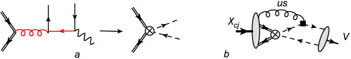
Figure 3: $(a)$ The illustration of the hard factorisation which gives the colour-octet operator. The red lines denote the hard propagators. The resulting operator has colour structure $\chi^{\dagger}_{\omega}T^{a}\psi_{\omega}\,\bar{q}_{hc}T^{a}q_{hc}$. The dashed lines denote the hard-collinear fields $q_{hc}$. $(b)$ The diagram which illustrates the formal factorisation of the hard-collinear modes. The black square denotes the subleading SCET vertex. The corresponding ultrasoft gluon is absorbed into the NRQCD matrix element with a colour-octet operator.

2.3 Decay amplitudes with transverse light meson.

For the final state with transverse meson one has to consider the twist-3 distribution amplitudes. There are two different possibilities: the photon is emitted from the light quark or from the heavy quark lines. Examples of the corresponding diagrams are shown in Fig.4.

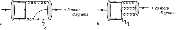
Figure 4: The leading order diagrams which provide contribution to the amplitude $A_{V}^{\bot}$.

The contributions with the three gluon DAs are possible only for the isosinglet mesons $\omega$ and $\phi$. All these contributions are of order $\alpha_{s}$ and the corresponding hard kernels are described by tree diagrams. Their analytical expressions are quite lengthy and we will not write them explicitly. The corresponding calculations are similar to the one described above and yield the following expressions

$$A_{0V}^{\bot} = i\left\langle\mathcal{O}(^{3}P_{0})\right\rangle\frac{f_{V}m_{V}}{M_{0}m^{4}}\sqrt{4\pi\alpha}\frac{\pi\alpha_{s}}{N_{c}}\int D\alpha_{i}\left\{\frac{Q_{V}}{\sqrt{6}}\frac{\left(2+\alpha_{3}\right)}{\alpha_{1}\alpha_{2}\alpha_{3}^{2}}\left(\frac{\alpha_{1}-\alpha_{2}}{1-\alpha_{3}}V(\alpha_{i})+A(\alpha_{i})\right)\right.$$ (53)

$$~{}\ \ \ \ \ \ \ \ \ \ \ \ \ \ \ \ \ \ \ \ \ \ \ \ \ \ \ \ \ \ \ \ \ \ \ \ \ \ \ \ \ \ \ \ \ \ \left.+~{}\delta_{I0}~{}e_{Q}2\sqrt{6}~{}\frac{G(\alpha_{i})}{\alpha_{1}\alpha_{2}\alpha_{3}}\frac{2+\alpha_{1}}{\alpha_{1}(1-\alpha_{1})}\right\},$$

$$A_{1V}^{\bot} = i\left\langle\mathcal{O}(^{3}P_{1})\right\rangle~{}\frac{~{}f_{V}m_{V}}{m^{5}}\frac{M_{1}^{2}}{m^{2}}\sqrt{4\pi\alpha}\frac{\pi\alpha_{s}}{N_{c}}\int D\alpha_{i}\left\{\delta_{I0}~{}9e_{Q}~{}\frac{G(\alpha_{i})}{\alpha_{1}\alpha_{2}\alpha_{3}^{2}}\right.$$ (54)

$$~{}\ \ \ \ \ \ \ \ \left.-\frac{Q_{V}}{4}\left(\frac{\alpha_{1}-\alpha_{2}}{\alpha_{1}\alpha_{2}\alpha_{3}^{2}}V(\alpha_{i})+\frac{1-\alpha_{3}}{\alpha_{1}\alpha_{2}\alpha_{3}^{2}}A(\alpha_{i})\right)\right\},$$

$$~{}A_{2V}^{\bot} = i\left\langle\mathcal{O}(^{3}P_{2})\right\rangle\frac{f_{V}m_{V}}{m^{5}}\frac{M_{2}}{m}\sqrt{4\pi\alpha}\frac{\pi\alpha_{s}}{N_{c}}\int D\alpha_{i}\left\{-\delta_{I0}3\sqrt{2}e_{Q}~{}\frac{G(\alpha_{i})}{\alpha_{1}\alpha_{2}\alpha_{3}^{2}}\right.$$ (55)

$$~{}\ \ \ \ \ \left.-\frac{Q_{V}}{4\sqrt{2}}\left(\frac{\alpha_{1}-\alpha_{2}}{\alpha_{1}\alpha_{2}\alpha_{3}^{2}}V(\alpha_{i})+\frac{1-\alpha_{3}}{\alpha_{1}\alpha_{2}\alpha_{3}^{2}}A(\alpha_{i})\right)\right\},$$

$$~{}T_{2V}^{\bot} = i\left\langle\mathcal{O}(^{3}P_{2})\right\rangle\frac{f_{V}m_{V}}{E_{\gamma}m^{4}}\frac{M_{2}}{E_{\gamma}}\sqrt{4\pi\alpha}\frac{\pi\alpha_{s}}{N_{c}}\int D\alpha_{i}\left\{-\delta_{I0}3\sqrt{2}e_{Q}\frac{G(\alpha_{i})}{\alpha_{1}\alpha_{2}\alpha_{3}^{2}}\frac{1}{1-\alpha_{3}}\right.$$ (56)

$$~{}\ \ \ \ \ \ \ \ \ \ \ \ \ \ \ \ \ \ \ \left.+\frac{Q_{V}}{2\sqrt{2}}\frac{1}{\alpha_{1}\alpha_{2}\alpha_{3}^{2}}\left(\frac{\alpha_{2}-\alpha_{1}}{1-\alpha_{3}}V(\alpha_{i})+A(\alpha_{i})\right)\right\}.$$

In these formulas it is implied that $e_{Q}$ is the electric charge of the heavy quark, the symbol $\delta_{I0}$ specifies the contribution which exists only for the meson states with isospin $I=0$. We also used the shorthand notation for the collinear integrals

$$\int D\alpha_{i}~{}f(\alpha_{i})=\int_{0}^{1}d\alpha_{1}\int_{0}^{1}d\alpha_{2}\int_{0}^{1}d\alpha_{3}~{}\delta(1-\alpha_{1}-\alpha_{2}-\alpha_{3})~{}f(\alpha_{1},\alpha_{2},\alpha_{3}),$$ (57)

The matrix element for the scalar charmonia reads

$$\left\langle 0\right|\frac{-1}{\sqrt{3}}~{}\chi_{\omega}^{{\dagger}}\left(\frac{-i}{2}\right)\overleftrightarrow{D}_{\top}^{\alpha}\gamma_{\top}^{\alpha}\psi_{\omega}~{}\left|\chi_{c0}\right\rangle=i\left\langle\mathcal{O}(^{3}P_{0})\right\rangle.$$ (58)

where the constant $\left\langle\mathcal{O}(^{3}P_{0})\right\rangle$ is given by expression in Eq.(31).

In order to describe the overlap with the transverse light mesons we need three-particle twist-3 DAs $V(\alpha_{i})$, $A(\alpha_{i})$ and $G(\alpha_{i})$. A detailed description of these nonperturbative functions is given in Appendix A. The properties of these functions allow one to conclude that the convolution integrals in Eqs.(53)-(56) are well defined.

The NRQCD matrix element in Eqs. (53)-(56) is of order $v^{4}$, the twist-3 operators in the collinear sector are of order $\lambda^{6}$. Therefore one finds

$$A_{iV}^{\bot}\sim T_{iV}^{\bot}\sim\alpha_{s}(\mu_{h})v^{4}\lambda^{4}.$$ (59)

Hence these amplitudes are suppressed by a factor $\lambda^{2}$ and enhanced by $\alpha_{s}$ compared to the longitudinal ones.

An appropriate contribution from the colour-octet operator is considered in Appendix B. We obtain that in the Coulomb limit the contribution from the colour-octet matrix element behaves as

$$\left[A_{1V}^{\bot}\right]_{oct}\sim\alpha_{s}(\mu_{h})\alpha_{s}(\mu_{us})\lambda^{4}v^{4}.$$ (60)

Hence following the same arguments as in the previous subsection and extrapolating this result to the real charmonium with $v\sim\lambda$ we expect that this contribution is of the same order as the singlet one

$$\left[A_{1V}^{\bot}\right]_{oct}/\left[A_{1V}^{\bot}\right]_{sing}\sim 1.$$ (61)

Therefore an estimate made with the help of the singlet contribution potentially may have a large uncertainty due to the colour-octet contribution.

3 Phenomenology

In this section we study numerical estimates using only contributions of the colour-singlet operators. Our aim is to understand how well one can describe the charmonium decays in this case using reliable estimates for various hadronic parameters.

In our numerical calculations we are using the following nonperturbative input. For the $c$-quark mass we take the value $m_{c}=1.5\$GeV, for the charmonium states $M_{0}=3.42\,$GeV, $M_{1}=3.51\,$GeV and $M_{2}=3.56\,$GeV and for the light mesons $m_{\rho}=775\,$MeV, $m_{\omega}=783\,$MeV, $m_{\phi}=1019\,$MeV. For the derivative of the radial wave function we use the value from Ref.[20] computed for the Buchmüller-Tye potential

$$|R_{21}^{\prime}(0)|^{2}=0.75\,\text{GeV}^{5}.$$ (62)

For the description of the light meson matrix elements we use the following values of the decay constants

$$f_{\rho}=221\,\text{MeV},~{}\ \ f_{\omega}=198\,\text{MeV},~{}\ \ f_{\phi}=161\,\text{MeV},$$ (63)

which are defined according to Eq.(A.2).

The estimates for the vector meson DAs have been studied in many works, see e.g. Refs.[21, 22, 23, 24]. The leading-order DA is described by the model with one parameter

$$\phi_{V}(x,\mu)=6x\bar{x}\left\{1+a_{2}^{V}(\mu)C_{2}^{3/2}(2x-1)\right\},$$ (64)

For the coefficients $a_{2}^{V}$ we use the values from Ref. [24]

$$a_{2}^{\rho}=a_{2}^{\omega}=0.15\pm 0.07,~{}a_{2}^{\phi}=0.18\pm 0.08,$$ (65)

where all parameters are given at the scale $\mu=1\,$GeV.

Using the explicit expressions for the coefficient functions $T_{i}(x)$ one can easily obtain the values for the convolution integrals

$$\int_{0}^{1}dx~{}\phi_{V}(x)T_{i}(x)=A_{i}+a_{2}^{V}(\mu_{h})~{}B_{i},$$ (66)

with

$$A_{i}=\int_{0}^{1}dx~{}6x\bar{x}~{}T_{i}(x),~{}\ B_{i}=\int_{0}^{1}dx~{}6x\bar{x}C_{2}^{3/2}(2x-1)~{}T_{i}(x).$$ (67)

Their numerical values read

$$A_{1} = 1.32+5.46i,~{}~{}\ A_{2}=-12.71+6.01i~{},~{}$$ (68)

$$\ B_{1} = 7.00+4.79i,~{}\ B_{2}=9.61+6.12i.$$ (69)

The transverse amplitudes depend on the twist-3 DAs defined in Eqs.(A.5)-(A.8) in Appendix A. For the quark-gluon DAs we use the models given in Eq.(A.15) which has been suggested in Refs.[21, 22, 23] . The nonperturbative parameters which enter in these formulas have been taken from Ref. [24] at the scale $\mu=1\,$GeV:

$$\rho~{}\text{and }\omega\text{-mesons} \zeta_{3}=0.030\pm 0.010,~{}\ \omega_{3}^{A}=-3.0\pm 1.4,~{}\ \omega_{3}^{V}=5.0\pm 2.4,$$ : (70)

$$\phi\text{-meson} \zeta_{3}=0.024\pm 0.008,~{}\ \omega_{3}^{A}=-2.6\pm 1.3,~{}\ \omega_{3}^{V}=5.3\pm 3.0~{}.$$ : (71)

In the following estimates we neglect the small difference for the $\phi$-meson and consider as a first guess that all parameters are constrained only by the values in Eq.(70).

For the isosinglet mesons $\omega$ and $\phi$ we have an additional contribution from the three gluon DAs. Taking into account the conformal expansion and mixing with the quark operators (see details in the Appendix) we use for them the models given in Eq.(A.17). We assume that the value of the corresponding local matrix element is small because we expect a very small pure gluon component of the meson wave function at low scale $\mu=1$GeV. Hence the constant $\omega_{3}^{G}$ must be much smaller then the corresponding constants of the quark gluon operators in Eq.(A.18) or

$$|\omega_{3}^{G}(\mu=1\text{GeV})|\ll 1.$$ (72)

We consider $\omega_{3}^{G}$ as a free parameter and try to estimate its value from the comparison with the data. The QCD evolution of all the twist-3 parameters is described in Appendix A.

The numerical results also depend on the choice of the hard scale $\mu_{h}$. In the following calculations it is fixed to be $\mu_{h}^{2}=2m_{c}^{2}$ if it is not written otherwise. For the total decay rates we used the data from Ref.[6]: $\Gamma_{tot}[\chi_{cJ}]=\{10.5,0.84,1.93\}$MeV for $J=0,1,2$, respectively. Finally, in the following calculations we use the NLO QCD coupling which has the value $\alpha_{s}(2m_{c}^{2})=0.290$

We start our discussion from the description of the branching rations $Br\left[\chi_{cJ}\rightarrow V_{\|}\gamma\right]$ because these observables are largest for $\chi_{c1}$ decays. The obtained results are given in Table 2.

	$\gamma\rho$	$\gamma\omega$	$\gamma\phi$
$\chi_{c1}\rightarrow V_{\|}\gamma$	$\begin{array}[]{cc}{}\hfil\\[-5.69054pt] 153.1_{-16.7-70.5}^{+18.2+103.7}\end{array}$	$13.6_{-1.5-6.3}^{+1.6+9.2}$	$31.3_{-3.8-14.5}^{+4.2+21.4}$
$\chi_{c2}\rightarrow V_{\|}\gamma$	$\begin{array}[]{cc}{}\hfil\\[-5.69054pt] 2.11_{-0.08-0.9}^{+0.09+1.3}\end{array}$	$0.19_{-0.007-0.08}^{+0.008+0.12}$	$0.41_{-0.02-0.18}^{+0.02+0.26}$

Table 2: The obtained values for the $Br\left[\chi_{c1,2}\rightarrow V_{\|}\gamma\right]$ in units of $10^{-6}$.

The first error shows the sensitivity to the value of the parameter $a_{2}^{V}$ within the intervals given in Eq.(65). The second error shows the dependence on $\mu_{h}$ within the interval $m_{c}<\mu_{h}<2m_{c}.$ The corresponding errors are large because the decay rates are proportional to the fourth power of the QCD coupling $Br\left[\chi_{c1}\rightarrow V_{\|}\gamma\right]\sim\alpha_{s}^{4}(\mu_{h})$. With the given estimate for $R^{\prime}_{21}(0)$ the obtained values for $Br\left[\chi_{c1}\rightarrow\rho_{\|}\gamma\right]$ and $Br\left[\chi_{c1}\rightarrow\phi_{\|}\gamma\right]$ are quite reliable although the obtained numbers lie somewhat below/above the experimental results given in Table 1. However, the estimate for $Br\left[\chi_{c1}\rightarrow\omega_{\|}\gamma\right]$ is about a factor of four smaller than the experimental value. One can also consider, for instance, the ratio $Br\left[\chi_{c1}\rightarrow\omega_{\|}\gamma\right]/Br\left[\chi_{c1}\rightarrow\rho_{\|}\gamma\right]$ in which the normalisation ambiguities cancel. If one assumes that the dominant contribution to the amplitudes arises from the terms associated with $u$ and $d$-quark components of the electromagnetic current in Eq.(3) then using $SU(2)$ symmetry one finds that this ratio must be

$$\frac{Br\left[\chi_{c1}\rightarrow\omega_{\|}\gamma\right]}{Br\left[\chi_{c1}\rightarrow\rho_{\|}\gamma\right]}\simeq\frac{1}{9},$$ (73)

However the experimental value for this ratio is $0.28$ which is about a factor of three larger. The large difference indicates that the assumption about the small contribution of the $c$-quark components in Eq.(1) is not valid. However the longitudinal amplitude in which the photon is emitted from a heavy quark $A^{\|}_{Q}$ can only be generated from a colour-octet operator. The basic idea is that one gluon in the diagram in Fig.1$(c)$ is ultrasoft while the other two are hard-collinear. These gluons create a light quark-antiquark pair in the octet state which after interaction with the ultasoft gluon becomes colorless, see also Fig. 7. In Appendix B we consider such colour-octet matrix element in the Coulomb limit. We obtain that such contribution behaves as

$$A_{Q}^{\|}\sim\alpha_{s}(\mu_{h})\alpha_{s}(\mu_{us})~{}\lambda^{2}v^{7}.$$ (74)

where we used the fact that $\alpha_{s}(\mu\sim mv)\sim v$, provides one more power of $v$. Following the same arguments as in Sec.2 we expect that for real charmonium with $v\sim\lambda$ this amplitude can be estimated as

$$A_{Q}^{\|}\sim\alpha_{s}(\mu_{h})\lambda^{2}v^{7}.$$ (75)

Therefore this amplitude is only suppressed by a factor $v$ compared to the colour-octet amplitude $[A^{\|}_{1V}]_{oct}$ in Eq.(52). We assume that the interference of this amplitude with the larger amplitudes $A^{\|}_{1V}$ and $[A_{V}^{\|}]_{oct}$ can be responsible for the large ratio in Eq.(73). Perhaps, these contributions strongly enhance the decay rate of the $\omega\gamma$ channel. One reason could be that the used value of $R^{\prime}_{21}(0)$ is somewhat large and therefore this numerically enhances the singlet contribution. In case the realistic value $R^{\prime}_{21}(0)$ is smaller, then the relative effect of the colour-octet contribution in the $\rho\gamma$ channel must be larger in order to describe the data. In any case it seems that the contribution of the colour-octet amplitude $A_{Q}^{\|}$ must play an important role in the correct description of the $\omega_{\|}\gamma$ decay mode.

The computed branching ratios for the state $\chi_{c2}$ are substantially smaller and they easily satisfy the experimental constraints. When comparing our results to Ref.[3], we note that our estimates for $\chi_{c1}$ shown in Table 2 are about an order of magnitude larger than theirs, while the results for the $\chi_{c2}$ decays are in good agreement.

We next consider the decay rates with transversely polarised mesons in the final state. The numerical evaluation with arbitrary twist-3 DA parameters (at scale $\mu=1$GeV) gives

$$\Gamma_{\rho}^{\bot}=222.4~{}\zeta_{3}^{2}(-9.82+4.78\omega_{3}^{A}+3.31\omega_{3}^{V})^{2},$$ (76)

$$\Gamma_{\omega}^{\bot}=181.2~{}\zeta_{3}^{2}(-3.3+1.4~{}\omega_{3}^{A}+8.3~{}\omega_{3}^{V}+735.6~{}\omega_{3}^{G})^{2},$$ (77)

$$\Gamma_{\phi}^{\bot}=168.7~{}\zeta_{3}^{2}(6.5-3.3~{}\omega_{3}^{A}+2.9~{}\omega_{3}^{V}+733.6~{}\omega_{3}^{G})^{2},$$ (78)

One can observe that the coefficients in front of the gluon parameter $\omega_{3}^{G}$ are always quite large, hence even the relatively small values of $\omega_{3}^{G}$ can produce a significant numerical impact. Formally, the large coefficient in Eqs.(77) and (78) arises due to the large normalization of the twist-3 gluon DA in Eq.(A.17).

The existing data do not allow us to fix the DA parameters in Eqs.(76)-(78) in order to unambiguously predict the decay widths for $\chi_{c0,2}$. From the numerical estimates we observe that there are different solutions which describe the data for $\chi_{c1}\rightarrow V_{\perp}\gamma$ decays within the experimental error bars and at the same time provide very different estimates for the $\chi_{c0,2}$ decays. In order to illustrate this let us consider a few examples. It is convenient to fix the parameters $\zeta_{3}$ and $\omega_{3}^{A}$ in accordance with the estimates in Eq.(70) and to study the possible restrictions on the two remaining constants $\omega_{3}^{V}=5.0\pm 2.4$ and $\left|\omega_{3}^{G}\right|<0.1$. The latter inequality must be considered as an assumption. For simplicity, for all final mesons $V$ we imply the value $a_{2}=0.22$ in the longitudinal amplitudes of $\chi_{c2}$ decays. In the following we consider two fixed values: $\zeta_{3}=0.03$ and $\zeta_{3}=0.04$. The different possible solutions for these values of $\zeta_{3}$ for a few different values of $\omega_{3}^{A}$ are shown in Fig.5.

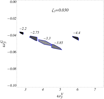
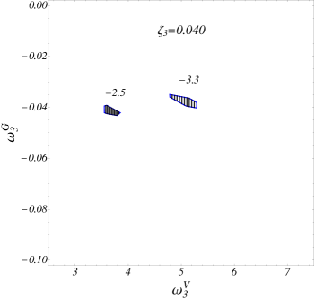
Figure 5: The numerical restrictions for the DA parameters $\omega_{3}^{V}$ and $\omega_{3}^{G}$ at fixed $\zeta_{3}$ and $\omega_{3}^{A}$ values (indicated on the allowed regions in both figures).

In the given regions we can describe the data for $\chi_{c1}$ satisfying the experimental constraints for the $\chi_{c0,2}$ decays. We observe that the strongest restrictions on the DA parameters are provided by the data for $\chi_{c1}$ decay. The restrictions on $\chi_{c2}$ decay rates are relatively weak but also allow us to get some constraints. The computed values for the decay widths of $\chi_{c0}$ are always so small that they do not contradict the experimental restrictions.

In Table 3 we show examples of the different values of parameters and corresponding results for the branching fractions.

				$\chi_{c1}\rightarrow V_{\perp}\gamma$			$\chi_{c2}\rightarrow V\gamma$			$\chi_{c0}\rightarrow V\gamma$
$\zeta_{3}$	$\omega_{3}^{A}$	$\omega_{3}^{V}$	$\omega_{3}^{G}$	$\rho$	$\omega$	$\phi$	$\rho$	$\omega$	$\phi$	$\rho$	$\omega$	$\phi$
0.03	-2.2	2.8	-0.037	29.6	20.8	4.8	3.4	0.18	2.6	2.0	0.17	0.66
0.03	-4.4	5.9	-0.043	30.0	13.9	8.5	17.2	3.7	6.5	0.40	0.05	0.15
0.04	-2.5	3.7	-0.041	39.2	13.5	6.5	7.1	0.40	5.6	1.9	0.16	0.54
0.04	-3.4	5.1	-0.038	33.2	14.2	6.2	16.3	3.6	6.50	0.62	0.09	0.23

Table 3: The examples of the DA parameters and the corresponding values of branching fractions in units of $10^{-6}$.

Note that we found the values of $\omega^{G}_{3}$ to be always negative, within this approach. We also observe that the twist-3 gluon contribution is critically important for a description of decays with $\omega$ and $\phi$ mesons. From the numerical results we find that

$$Br[\chi_{c1}\rightarrow\gamma\rho]>Br[\chi_{c2}\rightarrow\gamma\rho]>Br[\chi_{c0}\rightarrow\gamma\rho],$$ (79)

and

$$Br[\chi_{c2}\rightarrow\gamma\rho]>Br[\chi_{c2}\rightarrow\gamma\phi]>Br[\chi_{c2}\rightarrow\gamma\omega].$$ (80)

One can also see that there are solutions for which

$$Br[\chi_{c2}\rightarrow\gamma\phi]\geq Br[\chi_{c1}\rightarrow\gamma\phi].$$ (81)

The obtained results allow us to conclude that a further progress in our understanding of the radiative decays would come from a measurement of the branching for the $Br[\chi_{c2}\rightarrow\gamma\rho]$. It will also be interesting to carry out the corresponding helicity analysis. The estimates in Table 3 show that for the $\chi_{c2}$ decays the transverse branching fraction can be much larger the the longitudinal one; see Eq.(2). The dominant contribution is provided by the amplitude $T_{2\rho}^{\bot}$ which describes the decay of the charmonium state with helicity $\lambda=\pm 2$. Hence a prediction for the $Br[\chi_{c2}\rightarrow\gamma\rho]$ obtained only from the $\rho_{L}\gamma$ contribution can strongly underestimate the realistic value of the branching. Notice that for $\chi_{c1}$ decay the situation is opposite: the dominant amplitude is $A_{1\rho}^{\|}$ describing the decay of $\chi_{c1}(\lambda=\pm 1)$.

We also see that the used non-perturbative input and DAs models potentially allows one to describe the existing data for the transverse decays without the colour-octet contributions. If such a scenario is realised then the radiative decays can be used for a study of the twist-3 wave functions of the vector mesons. The future data on these decays will be helpful in order to reduce the ambiguities in the presented description and would allow us to further constrain the role of the various contributions.

4 Conclusions

In the present paper we studied the radiative decays of the $P$-wave charmonia $\chi_{cJ}\rightarrow\gamma V$ with $V=\rho,\omega,\phi$. The QCD factorisation has been used in a systematic way: NRQCD in the heavy meson sector and a collinear expansion in order to describe the overlap with light mesons in the final state. The colour-singlet contributions to all helicity amplitudes have been computed using the light-cone distribution amplitudes of twist-2 and twist-3. All obtained expressions are well defined at least in the leading-order approximation. The colour-octet contributions have also been studied in the Coulomb limit in order to obtain their scaling behaviour.

In order to understand the relevance of the different contributions we performed numerical estimates of the branching fractions using the colour-singlet approximations for the decay amplitudes. The various models for the vector meson distribution amplitudes which are available in the literature have been used in our numerical calculations.

Our results indicate that for the $\chi_{c1}\rightarrow\gamma V_{\|}$ decay the colour-singlet contributions alone do not allow to provide a reliable description of all branching fractions. In particular, the branching fraction for $\gamma\omega$ final state is about a factor four smaller than the observed value. We expect that the colour-octet matrix elements play an important role in this case. Qualitatively this conclusion also agrees with the observation that the ratio of the octet to singlet amplitudes behaves as $[A^{\|}_{1V}]_{octet}/[A^{\|}_{1V}]_{singlet}\sim v^{2}/\alpha_{s}(\mu\sim m_{c})$ which is not so small for charmonia. In addition, the $\omega\gamma$ decay amplitude might be enhanced by the specific gluonic colour-octet operator which can be responsible for the large ratio of the branching fractions for $\omega$ and $\rho$ mesons. We obtain that the corresponding amplitude is only suppressed by a factor of $v$ in comparison with the amplitude $[A^{\|}_{1V}]_{octet}$.

For decays with a transverse meson in the final state the singlet and octet operators contribute to the same order. Using only the singlet contributions we have shown that one can obtain a good description of the data but one needs to include the contributions with the three-gluon distribution amplitude which is quite sizeable in size. This observation may indicate a small color-octet contribution which would allow one to better constrain the twist-3 DAs of the vector mesons. We expect that future more precise measurements of the decay rates $\chi_{c2}\rightarrow V\gamma$ will help to reduce the theoretical uncertainties and further clarify the role of the various contributions in these reactions.

Appendix A Light-cone distribution amplitudes of the vector mesons

Here we briefly describe the properties of various distribution amplitudes which have been used in our calculations. For simplicity we use here the light-cone gauge

$$\bar{n}\cdot A(z)=0.$$ (A.1)

The required two-particle light-cone matrix elements read

$$\left\langle V(p)\right|\bar{q}(\lambda_{1}\bar{n})\gamma_{\mu}q(\lambda_{2}\bar{n})\left|0\right\rangle=(\epsilon_{V}^{\ast}\cdot\bar{n})\frac{1}{2}n^{\mu}~{}\sqrt{2}f_{V}m_{V}\int_{0}^{1}dx~{}\phi_{V}^{\|}(x)e^{i\lambda_{1}x\left(p\bar{n}\right)+i\lambda_{2}\bar{x}\left(p\bar{n}\right)}$$

$$+(\epsilon_{V}^{\ast})_{\mu_{\perp}}\sqrt{2}f_{V}m_{V}\int_{0}^{1}dx~{}g_{V}^{v}(x)e^{i\lambda_{1}x\left(p\bar{n}\right)+i\lambda_{2}\bar{x}\left(p\bar{n}\right)}$$ (A.2)

$$\left\langle V(p)\right|\bar{q}(\lambda_{1}\bar{n})\gamma_{\mu}\gamma_{5}q(\lambda_{2}\bar{n})\left|0\right\rangle=\frac{1}{2}i\varepsilon[\mu,\epsilon^{*}_{V},p,\bar{n}]\frac{1}{2}(\lambda_{1}-\lambda_{2})\sqrt{2}f_{V}m_{V}\int_{0}^{1}dx~{}g_{V}^{a}(x)e^{i\lambda_{1}x\left(p\bar{n}\right)+i\lambda_{2}\bar{x}\left(p\bar{n}\right)},$$ (A.3)

where we neglected the contributions of twist-4. For all operators in this paper we assume an appropriate flavour structure

$$\left\langle\rho^{0}\right|(\bar{u}u-\bar{d}d)\left|0\right\rangle,\ \left\langle\omega\right|(\bar{u}u+\bar{d}d)\left|0\right\rangle,\ \left\langle\phi\right|\bar{s}s\left|0\right\rangle.$$ (A.4)

The required three-particle twist-3 matrix elements are given by (recall that $p_{-}\equiv(p\bar{n})$)

$$\left\langle V(p)\right|\bar{q}(\lambda_{1}\bar{n})g\tilde{G}_{\bar{n}\nu}(\lambda_{3}\bar{n})\hbox to0.0pt{\hbox to5.00002pt{\hfil$\bar{n}$\hfil}\hss}/\gamma_{5}q(\lambda_{2}\bar{n})\left|0\right\rangle=-\sqrt{2}f_{V}m_{V}\left(\epsilon_{V}^{\ast}\right)_{\nu}p_{-}^{2}~{}\mathcal{A}(\lambda_{i}p_{-}),$$ (A.5)

$$\left\langle V(p)\right|\bar{q}(\lambda_{1}\bar{n})gG_{\bar{n}\nu}(\lambda_{2}\bar{n})\hbox to0.0pt{\hbox to5.00002pt{\hfil$\bar{n}$\hfil}\hss}/q(\lambda_{3}\bar{n})\left|0\right\rangle=i\sqrt{2}f_{V}m_{V}\left(\epsilon_{V}^{\ast}\right)_{\nu}p_{-}^{2}~{}\mathcal{V}(\lambda_{i}p_{-}),$$ (A.6)

$$\left\langle V(p)\right|~{}gd^{abc}G_{\bar{n}\xi}^{a}(\lambda_{1}\bar{n})G_{\bar{n}}^{b\xi}(\lambda_{2}\bar{n})G_{\bar{n}\nu}^{c}(\lambda_{3}\bar{n})\left|0\right\rangle=i\sqrt{2}f_{V}m_{V}(\epsilon^{\ast})_{\nu}p_{-}^{3}~{}\mathcal{G}(\lambda_{i}),$$ (A.7)

$$\left\langle V(p)\right|gd^{abc}G_{\bar{n}\xi}^{a}(\lambda_{1}\bar{n})\tilde{G}_{\bar{n}}^{b\xi}(\lambda_{2}\bar{n})\tilde{G}_{\bar{n}\nu}^{c}(\lambda_{3}\bar{n})\left|0\right\rangle=-i\sqrt{2}f_{V}m_{V}(\epsilon^{\ast})_{\nu}p_{-}^{3}~{}\mathcal{\tilde{G}}(\lambda_{i}),$$ (A.8)

where $d^{abc}$ is the fully symmetrical structure constant of the $SU(3)$ colour group and

$$G_{\bar{n}\xi}^{a}(z)=\bar{n}^{\alpha}G_{\alpha\xi}^{a}(z),~{}\tilde{G}_{\bar{n}\xi}^{a}=\frac{1}{2}\varepsilon_{\alpha\xi\mu\nu}\bar{n}^{\alpha}G^{\mu\nu}(z).$$ (A.9)

The vector decay couplings $f_{V}$ can be obtained from the leptonic decays. Their explicit values are given in Eq.(63).

All functions on the $rhs$ of Eqs. (A.5)-(A.8) can be presented as

$$\mathcal{A(V,\mathcal{G,\tilde{G}})}(\lambda_{i}p_{-})=\int D\alpha_{i}~{}A(V,G,\tilde{G})(\alpha_{i})e^{i\left(p\bar{n}\right)(\lambda_{1}\alpha_{1}+\lambda_{2}\alpha_{2}+\lambda_{3}\alpha_{3})},$$ (A.10)

with the integration measure $D\alpha_{i}$ defined in Eq.(57).

The properties of the DAs, except the pure gluonic ones, have been discussed in Refs.[21, 22, 23, 24]. The two-particle functions are symmetrical with respect to exchange $x\leftrightarrow\bar{x}$ and normalised as

$$\phi_{V}^{\|}(1-x)=\phi_{V}^{\|}(x),\ g^{v,a}_{V}(1-x)=g^{v,a}_{V}(x),$$ (A.11)

$$\int_{0}^{1}dx\ \phi_{V}^{\|}(x)=\int_{0}^{1}dxg^{v,a}_{V}(x)=1.$$ (A.12)

The QCD equation of motions and operator identities allow one to express the twist-3 DAs $g^{v,a}_{V}$ in terms of $\phi_{V}^{\|}$ and twist-3 functions $V$ and $A$, see e.g. [22]. Neglecting the three-particle contributions with $V$ and $A$ one has

$$g_{V}^{v}(x)=\frac{1}{2}\int_{0}^{x}dv\frac{\phi_{V}^{\|}(v)}{\bar{v}}+\frac{1}{2}\int_{x}^{1}dv\frac{\phi_{V}^{\|}(v)}{v},$$ (A.13)

$$g^{a}_{V}(x)=2\bar{x}\int_{0}^{x}dv\frac{\phi_{V}^{\|}(v)}{\bar{v}}+2x\int_{x}^{1}dv\frac{\phi_{V}^{\|}(v)}{v}.$$ (A.14)

These expressions are often referred to as the Wandzura-Wilczeck approximation.

The models for the functions $V$, $A$ have been constructed using the conformal expansion, see details in Ref. [22]. Corresponding functions include the contributions from local operators with conformal spin $j=7/2$ and $j=9/2$ and read

$$A(\alpha_{i})=360\zeta_{3}\alpha_{1}\alpha_{2}\alpha_{3}^{2}\left(1+\omega_{3}^{A}\frac{1}{2}\left(7\alpha_{3}-3\right)\right),\quad V(\alpha_{i})=540\zeta_{3}\omega_{3}^{V}\alpha_{1}\alpha_{2}\alpha_{3}^{2}(\alpha_{2}-\alpha_{1}),$$ (A.15)

The quark-gluon operators in our case mix with the pure gluonic ones. Moreover, at the leading-logarithmic approximation such mixing is possible only for the operators with equal conformal spin. Hence constructing the models for the gluon DAs $G$ and $\tilde{G}$ we consider only the contributions with the same conformal spin as for the quark-gluon DAs. From the definitions of the operators in Eqs.(A.7) and (A.8) one can see that

$$G(\alpha_{2},\alpha_{1},\alpha_{3})=G(\alpha_{1},\alpha_{2},\alpha_{3}),\ \ \tilde{G}(\alpha_{2},\alpha_{1},\alpha_{3})=-\tilde{G}(\alpha_{1},\alpha_{2},\alpha_{3}).$$ (A.16)

Using this information and following the arguments as in Ref.[22] one obtains that the conformal expansion of the function $G$ and $\tilde{G}$ is starting from the conformal spin $j=9/2$ and $j=11/2$, respectively. However as soon as contributions with the spin $j\geq 11/2$ in $V$ and $A$ have been neglected we assume that $\tilde{G}(\beta_{i})$ can also be neglected. Therefore

$$G(\alpha_{i})=5040~{}\zeta_{3}\omega_{3}^{G}\alpha_{1}^{2}\alpha_{2}^{2}\alpha_{3}^{2},\quad\tilde{G}(\alpha_{i})\simeq 0.$$ (A.17)

The twist-3 DAs have the following normalization

$$\int D\alpha_{i}A(\alpha_{i})=\zeta_{3},~{}~{}\int D\alpha_{i}(\alpha_{2}-\alpha_{1})V(\alpha_{i})=\zeta_{3}\omega_{3}^{V}\ ,~{}~{}\int D\alpha_{i}G(\alpha_{i})=\zeta_{3}\omega_{3}^{G}.$$ (A.18)

In general, the parameters $\zeta_{3}$ and $\omega_{3}^{A,V,G}$ are different for the $\rho,\ \omega$ and $\phi$ mesons. For the sake of simplicity we neglect this difference at low scale $\mu_{0}=1$GeV in our numerical calculations and assume

$$\left.\zeta_{3}(1\text{GeV})\right|_{\rho}=\left.\zeta_{3}(1\text{GeV})\right|_{\omega}=\left.\zeta_{3}(1\text{GeV})\right|_{\phi},$$ (A.19)

$$\left.\omega_{3}^{A,V}(1\text{GeV})\right|_{\rho}=\left.\omega_{3}^{A,V}(1\text{GeV})\right|_{\omega}=\left.\omega_{3}^{A,V}(1\text{GeV})\right|_{\phi},$$ (A.20)

$$\left.\omega_{3}^{G}(1\text{GeV})\right|_{\omega}=\left.\omega_{3}^{G}(1\text{GeV})\right|_{\phi}.$$ (A.21)

Therefore we do not write an additional index associated with the mesonic state assuming that this information is clear from the context.

All distribution amplitude parameters have to be evolved from the low scale $\mu_{0}=1$GeV to some hard scale $\mu\sim m$. The evolution of the twist-2 coupling $a_{2}^{V}$ is simple and well known, see e.g. Ref.[21]. The evolution of the twist-3 DAs is more complicated and we take a closer look at it. The evolution of the coupling $\zeta_{3}$ (the lowest conformal spin $j=7/2$) is also simple and for all mesons one has, see e.g. [23]

$$\zeta_{3}(\mu)=\left(\frac{\alpha_{s}(\mu)}{\alpha_{s}(\mu_{0})}\right)^{{\gamma}_{00}/b}\zeta_{3}(\mu_{0}),$$ (A.22)

with the anomalous dimension

$$\gamma_{00}=-\frac{1}{3}C_{F}+3C_{A},$$ (A.23)

and $b=\frac{11}{3}N_{c}-\frac{2}{3}n_{f}$. As the parameters $\omega_{3}^{V,A}$ are mixing ($j=9/2$), we introduce

$$\boldsymbol{\omega}_{3}(\mu)=\left(\begin{array}[c]{c}\omega_{3}^{A}(\mu)\\ \omega_{3}^{V}(\mu)\end{array}\right).$$ (A.26)

For the $\rho$ meson one then has

$$\rho\text{-meson}\quad\boldsymbol{\omega}_{3}(\mu)=\left(\frac{\alpha_{s}(\mu)}{\alpha_{s}(\mu_{0})}\right)^{\hat{\gamma}_{(8)}/b}\boldsymbol{\omega}_{3}(\mu_{0}),$$ (A.27)

with the $2\times 2$ anomalous dimension matrix $\hat{\gamma}_{(8)}$ which will be given below.

The evolution of the corresponding parameters for the $\omega$ and $\phi$ is more involved because of mixing with the gluon coupling $\omega_{3}^{G}$ and due to the flavour mixing. Performing the evolution of the twist-3 parameters $\zeta_{3}$, $\omega_{3}^{V,A,G}$ we assume that at low scale $\mu=1$GeV, $\omega\sim(u\bar{u}+d\bar{d})$ and $\phi\sim s\bar{s}$ and therefore the matrix elements with $s$- and $u(d)$-quarks vanish, respectively. Our results for the evolved couplings read

$$\omega\text{-meson }\quad\boldsymbol{\omega}_{3}(\mu)=\frac{1}{\sqrt{3}}\boldsymbol{\omega}_{3}^{(8)}(\mu)+\sqrt{\frac{2}{3}}\boldsymbol{\omega}_{3}^{(1)}(\mu),$$ (A.28)

$$\phi\text{-meson }\quad\boldsymbol{\omega}_{3}(\mu)=-\sqrt{\frac{2}{3}}\boldsymbol{\omega}_{3}^{(8)}(\mu)+\frac{1}{\sqrt{3}}\boldsymbol{\omega}_{3}^{(1)}(\mu),$$ (A.29)

where

$$\boldsymbol{\omega}_{3}^{(8)}(\mu)=\left(\frac{\alpha_{s}(\mu)}{\alpha_{s}(\mu_{0})}\right)^{\hat{\gamma}_{(8)}/b}\boldsymbol{\omega}_{3}^{(8)}(\mu_{0}),\quad\left(\begin{array}[c]{c}\boldsymbol{\omega}_{3}^{(1)}(\mu)\\ \omega_{3}^{G}(\mu)\end{array}\right)=\left(\frac{\alpha_{s}(\mu)}{\alpha_{s}(\mu_{0})}\right)^{\hat{\gamma}_{(1)}/b}\left(\begin{array}[c]{c}\boldsymbol{\omega}_{3}^{(1)}(\mu_{0})\\ \omega_{3}^{G}(\mu_{0})\end{array}\right),$$ (A.34)

with the appropriate initial conditions

$$\omega\text{-meson }\quad\boldsymbol{\omega}_{3}^{(8)}(\mu_{0})=\frac{1}{\sqrt{3}}\boldsymbol{\omega}_{3}(\mu_{0}),\quad\boldsymbol{\omega}_{3}^{(1)}(\mu_{0})=\sqrt{\frac{2}{3}}\boldsymbol{\omega}_{3}(\mu_{0}),$$ (A.35)

$$\phi\text{-meson }\quad\boldsymbol{\omega}_{3}^{(8)}(\mu_{0})=-\sqrt{\frac{2}{3}}\boldsymbol{\omega}_{3}(\mu_{0}),\quad\boldsymbol{\omega}_{3}^{(1)}(\mu_{0})=\frac{1}{\sqrt{3}}\boldsymbol{\omega}_{3}(\mu_{0}).$$ (A.36)

The anomalous dimension matrices in Eqs.(A.27) and (A.34) read

$$\hat{\gamma}_{(8)}=\left(\begin{array}[c]{cc}\gamma_{AA}-\gamma_{00}&\gamma_{AV}\\ \gamma_{VA}&\gamma_{VV}-\gamma_{00}\end{array}\right),\ \ \ \hat{\gamma}_{(1)}=\left(\begin{array}[c]{ccc}\gamma_{AA}-\gamma_{00}&\gamma_{AV}&0\\ \gamma_{VA}&\gamma_{VV}-\gamma_{00}&\frac{56}{3}\gamma_{VG}\\ 0&-\frac{3}{56}\gamma_{GV}&\gamma_{GG}-\gamma_{00}\end{array}\right).$$ (A.37)

The values of $\gamma_{ij}$ are related with the renormalisation of the corresponding operators. Their values have been obtained from the evolution kernels computed in Ref. [25]:

$$~{}\gamma_{AA}=\frac{1}{4}C_{F}+\frac{25}{6}C_{A},~{}~{}\gamma_{AV}=-\frac{3}{4}C_{F}+\frac{1}{2}C_{A},$$ (A.38)

$$~{}\gamma_{VA}=-\frac{7}{4}C_{F}+\frac{7}{6}C_{A},~{}~{}\gamma_{VV}=\frac{31}{12}C_{F}+\frac{13}{6}C_{A},~{}~{}\gamma_{VG}=-\frac{n_{f}}{3},$$ (A.39)

$$\gamma_{GV}=\frac{8}{3}\left(8C_{F}-3C_{A}\right),~{}~{}\ \gamma_{GG}\mathcal{=}3C_{A}+\frac{2}{3}n_{f}.$$ (A.40)

We have checked that Eq.(A.27) describing the evolution of the $\rho$-meson DAs is in agreement with the expression given in Ref.[23].

Appendix B Colour-octet corrections in the Coulomb limit

In this section we consider various colour-octet contributions which potentially can provide a sizable correction to the amplitudes derived in the previous sections. The relevance of the colour-octet mechanism in decays of $P$-wave charmonia has been discussed in various papers, see e.g. Refs.[8, 9, 10]. In this appendix we only focus on decays $\chi_{c1}\rightarrow V\gamma$ since the corresponding branching rates are already known from experiments.

We start our discussion from the longitudinal amplitude $A_{1V}^{\|}$ which is suppressed by $\alpha_{s}^{2}$. In this case the large correction can be generated by the ultrasoft region where one of the gluons in the diagram in Fig.2 is ultrasoft. Although such contribution might be suppressed by a small factor $v^{2}$ the corresponding hard kernel is of order $\alpha_{s}$. In order to simplify our discussion we consider the Coulomb limit when $mv^{2}\gg$ $\Lambda$. In this case the scales $v$ and $\lambda$ are well separated $v^{2}\gg\lambda^{2}$ and the charmonium state can be considered as a perturbative Coulomb state.

The simplest way to obtain the subleading amplitude $\left[A_{1V}^{\|}\right]_{oct}\sim\alpha_{s}(\mu)v^{6}$ is just to consider the ultrasoft limit $k\sim mv^{2}$ in Eq.(32) and to expand the integrand with respect to small momentum $k$. In the effective theory such a limit can be associated with the integration over soft gluons with momenta $k_{s}\sim mv.$ This reduces the description of the heavy quark sector to potential NRQCD (PNRQCD)[26, 27, 28, 29, 30]. Schematically, the factorisation can be described in the following way. First we integrate over hard modes and obtain the effective theory which consists of two sectors: nonrelativistic associated with the heavy quarks and collinear associated with collinear light particles. The effective Lagrangian is given by the sum of the NRQCD and SCET-I($v$) Lagrangians. The latter describes the interactions of the ultrasoft $k_{us}\sim m(v^{2},v^{2},v^{2})$ and hard-collinear particles with momenta $p_{hc}=(\bar{n}\cdot p_{hc},n\cdot p_{hc},~{}p_{\perp hc})\sim m(1,v^{2},v).$ At the next step we integrate out the soft gluon modes ( $k_{s}^{\mu}\sim mv$) in NRQCD reducing it to PNRQCD . To proceed further we integrate over the hard-collinear particles $p_{hc}\sim m(1,v^{2},v)$ and over ultrasoft modes $k_{us}\sim m(v^{2},v^{2},v^{2})$ which are still perturbative degrees of freedom. After that we reduce our description to the effective Lagrangian with $\lambda$-collinear particles with momenta $p_{c}\sim m(1,\lambda^{4},\lambda^{2})$. Only these degrees of freedom can describe an overlap with the external collinear hadronic states.

In the following we are not going to build a detailed approach for the description of the colour-octet contributions. Our task is rather modest: we would only like to demonstrate the existence of the colour-octet contributions with a certain power behaviour. For that purpose we do not need to perform all required matching calculations in the framework of effective theory. Instead, we are going to proceed as follows. We assume that the annihilation of heavy quarks to a hard gluon is described by simple hard vertex graph and this gives the NRQCD colour-octet operator

$$\mathcal{O}^{8}(^{3}S_{1})=\chi_{\omega}^{{\dagger}}\gamma_{\top}^{\beta}T^{a}\psi_{\omega}.$$ (B.1)

The further calculations in the heavy quark sector will be carried out within the PNRQCD framework. The subprocesses associated with hard and hard-collinear scattering will be computed just by expansion with respect to the small ultrasoft momentum of the corresponding subgraph in QCD. In other words in these sectors we apply the technique known as expansion by regions [28, 31]. This allows us to avoid a detailed discussion of the SCET formalism and the corresponding matching calculations. The structure of the resulting diagram is shown in Fig.6.

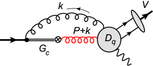
Figure 6: The diagram describing the colour-octet mechanism in the effective theory. $G_{c}$ is the octet propagator in PNRQCD. The hard gluon is shown by a red curly line. The crossed circle denotes the vertex of the octet operator (B.1).

The corresponding analytical expression reads

$$i\varepsilon[\epsilon_{\chi},\epsilon_{\gamma}^{\ast},p,q]~{}(\epsilon_{V}^{\ast}\cdot\omega)\frac{m_{V}}{M_{1}^{2}}\left[A_{1V}^{\|}\right]_{oct}=2(\epsilon_{V}^{\ast}\cdot\omega)Q_{V}\sqrt{2}~{}f_{V}~{}m_{V}\int_{0}^{1}dx~{}\phi_{\|}^{V}(x)$$

$$\times\int dk~{}\frac{\left(-i\right)^{2}\text{Tr}[\mathcal{P}_{V}~{}D_{q}^{\alpha\beta}]}{\left[k^{2}\right]\left[4m^{2}\right]}\sqrt{\frac{M}{N_{c}}}\int\frac{d^{3}\boldsymbol{\Delta}}{(2\pi)^{3}}\sqrt{\frac{3}{4\pi}}\tilde{R}_{21}(|\boldsymbol{\Delta}|)\frac{1}{4}\text{Tr}\left[\mathcal{P}_{1}(1-\omega)D^{Q}_{\alpha\beta}(E,\Delta_{\top},k)(1+\omega)\right],$$ (B.2)

where $D_{q}^{\alpha\beta}$ denotes the subgraph with hard and hard-collinear interactions between light quarks and photons, the indices $\alpha$ and $\beta$ are associated with the gluons ( ultrasoft and hard). In full QCD it is described by the same expression as in Eq.(36). Now we assume that the gluon momentum $k$ is ultrasoft and $D_{q}$ must be expanded in $k$. The second trace with subgraph $D^{Q}$ describes the heavy quark sector in PNRQCD and $R_{21}(|\Delta|)$ is the Coulomb radial wave function in momentum space, see e.g. [10],

$$\tilde{R}_{21}(|\boldsymbol{\Delta}|)=-iR_{21}^{\prime}(0)\frac{1024\pi\gamma_{B}|\boldsymbol{\Delta}|}{\left(4\boldsymbol{\Delta}^{2}+\gamma_{B}^{2}\right)^{3}},~{}\ \gamma_{B}=\frac{1}{2}m_{c}\alpha_{s}C_{F}.$$ (B.3)

Many technical details have already been discussed in the literature (see e.g. Refs.[13, 10, 32]); therefore we do not describe them here. The $P$-wave projector reads

$$\mathcal{P}_{1}=\frac{1}{2\sqrt{2}}\frac{\Delta_{\top}^{\sigma}}{|\Delta_{\top}|}\left[\gamma_{\sigma},\leavevmode\hbox{\hbox to0.0pt{\thinspace/\hss}{$\epsilon$}}_{\chi}\right]\gamma_{5}.$$ (B.4)

The analytical expression for the $D_{\alpha\beta}^{Q}$ in Eq.(B.2) is given by

$$D_{\alpha\beta}^{Q}(E,\Delta_{\top},k)=\int\frac{d^{3}\mathbf{\Delta}^{\prime}}{(2\pi)^{3}}~{}\left[V_{\mathcal{O}}^{\beta,b}\right]~{}iG_{c}^{(8)}\left[\Delta_{\top}^{\prime},\Delta_{\top}+k_{\top},E+(k\omega)\right]~{}\left[V_{g}^{\alpha,a}\right],$$ (B.5)

where $V_{\mathcal{O}}^{\rho,a}$ and $V_{g}^{\alpha,b}$denote the operator and ultrasoft gluon vertices, respectively. For the colour-octet Coulomb Green function $G_{c}^{(8)}$ we use the simplified expression suggested in Ref.[10]

$$iG_{c}^{(8)}\left[\Delta_{\top}^{\prime},\Delta_{\top}+k_{\top},E+(k\omega)\right]\simeq\frac{(-i)}{E+(k\omega)+\Delta_{\top}^{2}/m+i\varepsilon}(2\pi)^{3}\delta(\Delta_{\top}^{\prime}-\Delta_{\top}).$$ (B.6)

The ultrasoft gluon vertex $V_{g}$ is generated by the chromoelectric dipole interaction in the effective PNRQCD Lagrangian

$$\mathcal{L}_{int}=g\int d^{3}\mathbf{x}~{}S_{\omega}^{{\dagger}}(\mathbf{x})\left[~{}\vec{x}\cdot\vec{E}(t,0)\right]~{}O_{\omega}(\mathbf{x}),$$ (B.7)

where $S_{\omega}$ and $O_{\omega}$ denote the quark-antiquark singlet and octet fields, respectively, see e.g. [13]. In momentum space this gives

$$D^{Q}_{\alpha\beta}(E,\Delta_{\top},k) = \left[igT^{b}\gamma_{\top\beta}\right]_{V_{\mathcal{O}}}~{}\left[gT^{a}\left\{\omega_{\alpha}k_{\top\lambda}-g_{\top\alpha\lambda}(\omega k)\right\}\frac{\partial}{\partial\Delta_{\top}^{\lambda}}\right]_{V_{g}}\frac{(-i)}{\left[E+(k\omega)+\Delta_{\top}^{2}/m+i\varepsilon\right]}$$ (B.8)

$$= \left[igT^{b}\gamma_{\top\beta}\right]_{V_{\mathcal{O}}}~{}gT^{a}\left\{\omega_{\alpha}k_{\top\lambda}-g_{\top\alpha\lambda}(\omega k)\right\}\frac{(-2)}{m}\frac{i\Delta_{\top}^{\lambda}}{\left[E+(k\omega)+\Delta_{\top}^{2}/m+i\varepsilon\right]^{2}}.$$

The trace in Eq.(B.2) yields

$$\frac{1}{4}\text{Tr}\left[\mathcal{P}_{1}(1-\omega)D^{Q}_{\alpha\beta}(E,\Delta_{\top})(1+\omega)\right]=\frac{\delta^{ab}}{2}\frac{g\left\{\omega_{\alpha}k_{\top\lambda}-g_{\top\alpha\lambda}(\omega k)\right\}}{\left[E+(k\omega)+\Delta_{\top}^{2}/m+i\varepsilon\right]^{2}}\frac{2}{m}\frac{1}{\sqrt{2}}\frac{\Delta_{\top}^{\lambda}\Delta_{\top}^{\sigma}}{|\Delta_{\top}|}i\varepsilon[\omega\epsilon_{\chi}\sigma\beta],$$ (B.9)

and we obtain

$$~{}\int\frac{d^{3}\boldsymbol{\Delta}}{(2\pi)^{3}}\tilde{R}_{21}(|\mathbf{\Delta}|)\frac{1}{4}\text{Tr}\left[\mathcal{P}_{1}(1-\omega)D^{Q}_{\alpha\beta}(E,\Delta_{\top},k)(1+\omega)\right]$$

$$=-\frac{\delta^{ab}}{\sqrt{2}}\ \frac{g}{3m}\int\frac{d^{3}\boldsymbol{\Delta}}{(2\pi)^{3}}|\boldsymbol{\Delta}|\tilde{R}_{21}(|\mathbf{\Delta}|)\frac{i\varepsilon[\omega\epsilon_{\chi}\sigma\beta]\left\{\omega_{\alpha}k_{\top}^{\sigma}-(g_{\top})_{\alpha}^{\sigma}(\omega k)\right\}}{\left[E+(k\omega)+\Delta_{\top}^{2}/m+i\varepsilon\right]^{2}},$$ (B.10)

where we used rotational invariance in order to rewrite  $\Delta_{\top}^{\lambda}\Delta_{\top}^{\sigma}\rightarrow-|\mathbf{\Delta}|^{2}g_{\top}^{\lambda\sigma}/3$. Substituting this into Eq.(B.2) and computing the colour trace we obtain

$$i\varepsilon[\epsilon_{\chi},\epsilon_{\gamma}^{\ast},p,q]~{}(\epsilon_{V}^{\ast}\cdot\omega)\frac{m_{V}}{M_{1}^{2}}\left[A_{1V}^{\|}\right]_{oct}=(\epsilon_{V}^{\ast}\cdot\omega)Q_{V}\frac{if_{V}m_{V}}{m^{3}}\sqrt{\frac{M}{N_{c}}}\sqrt{\frac{3}{4\pi}}\frac{C_{F}}{6\pi^{2}}\alpha_{s}(\mu_{h})\alpha_{s}(\mu_{us})$$

$$\times\int_{0}^{1}dx~{}\phi_{\|}^{V}(x)\int\frac{d^{3}\mathbf{\Delta}}{(2\pi)^{3}}|\boldsymbol{\Delta}|\tilde{R}_{21}(|\mathbf{\Delta}|)\int d^{4}k~{}\frac{\text{Tr}[\mathcal{P}_{V}~{}D_{q}^{\alpha\beta}]}{\left[k^{2}\right]}\frac{i\varepsilon[\omega\epsilon_{\chi}\sigma\beta]g\left\{\omega_{\alpha}k_{\top}^{\sigma}-(g_{\top})_{\alpha}^{\sigma}(\omega k)\right\}}{\left[E+(k\omega)+\Delta_{\top}^{2}/m+i\varepsilon\right]^{2}},~{}$$ (B.11)

where the Lorentz indices $\alpha$ and $\beta$ correspond to the ultrasoft and hard (i. e. colour-octet operator) gluon respectively. The expansion of the light quark term Tr$[\mathcal{P}_{V}~{}D_{q}]$ is carried out by expanding the hard-collinear and hard propagators to the next-to-leading order

$$\frac{(p_{i}+k)}{\left[(p_{i}+k)^{2}\right]}\simeq\frac{\leavevmode\hbox{\hbox to0.0pt{\thinspace/\hss}{$p$}}_{i}}{\left[2(kp_{i})\right]}+\frac{\leavevmode\hbox{\hbox to0.0pt{\thinspace/\hss}{$k$}}}{\left[2(kp_{i})\right]}-\frac{k^{2}}{\left[2(kp_{i})\right]^{2}},$$ (B.12)

$$\frac{\leavevmode\hbox{\hbox to0.0pt{\thinspace/\hss}{$p$}}_{i}+\leavevmode\hbox{\hbox to0.0pt{\thinspace/\hss}{$q$}}+\leavevmode\hbox{\hbox to0.0pt{\thinspace/\hss}{$k$}}}{\left[\left(p_{i}+q+k\right)^{2}\right]}\simeq\frac{\left(\leavevmode\hbox{\hbox to0.0pt{\thinspace/\hss}{$p$}}_{i}+\leavevmode\hbox{\hbox to0.0pt{\thinspace/\hss}{$q$}}\right)}{\left[2\left(p_{i}q\right)\right]}+\frac{\leavevmode\hbox{\hbox to0.0pt{\thinspace/\hss}{$k$}}}{\left[2\left(p_{i}q\right)\right]}-\frac{\left(\leavevmode\hbox{\hbox to0.0pt{\thinspace/\hss}{$p$}}_{2}+\leavevmode\hbox{\hbox to0.0pt{\thinspace/\hss}{$q$}}\right)}{\left[2\left(p_{i}q\right)\right]}\frac{2k(p+q)}{\left[2\left(p_{i}q\right)\right]},$$ (B.13)

where $p_{i}=\{xp,\bar{x}p\}$. The result can be written as

$${\text{Tr}[\mathcal{P}_{V}~{}D_{q}^{\alpha\beta}]} \simeq \frac{1}{\left[8m^{3}\right]}\frac{1}{\left[(kp)\right]}\left(p^{\beta}\left\{p^{\alpha}(\varepsilon_{\gamma}k)-\varepsilon_{\gamma}^{\alpha}(kp)\right\}\frac{2}{x}\right.$$ (B.14)

$$+q^{\beta}\left\{(\varepsilon_{\gamma}k)p^{\alpha}-(kp)\varepsilon_{\gamma}^{\alpha}\right\}\frac{1-2x}{2x^{2}}+\varepsilon_{\gamma}^{\beta}\left\{(kp)q^{\alpha}-p^{\alpha}(kq)\right\}\frac{3-2x}{2x^{2}}$$

$$\left.+\left[(pq)\left\{\varepsilon_{\gamma}^{\alpha}k^{\beta}-g^{\alpha\beta}(\varepsilon_{\gamma}k)\right\}+p^{\beta}\left\{q^{\alpha}(\varepsilon_{\gamma}k)-\varepsilon_{\gamma}^{\alpha}(kq)\right\}\right]\frac{1+2x}{2x^{2}}\right)+\left(x\rightarrow\bar{x}\right).$$

Notice that this expression vanishes if it is contracted with the ultrasoft gluon momentum $k^{\alpha}$,

$${k_{\alpha}\text{Tr}[\mathcal{P}_{V}~{}D_{q}^{\alpha\beta}]}=0,$$ (B.15)

as it is required by the gauge invariance. Substituting this into Eq.(B.11) and performing contractions of the Lorentz indices we obtain

$$\left[A_{1V}^{\|}\right]_{oct}\sim\alpha_{s}(\mu_{h})\alpha_{s}(\mu_{us})~{}\frac{f_{V}M_{1}^{2}}{m^{6}}\sqrt{M_{1}}\int_{0}^{1}dx~{}\frac{\phi_{\|}^{V}(x)}{x}\int\frac{d^{3}\mathbf{\Delta}}{(2\pi)^{3}}~{}\tilde{R}_{21}(|\mathbf{\Delta}|)|\mathbf{\Delta}|~{}J_{us},$$ (B.16)

with

$$J_{us}=\int dk~{}\frac{1}{\left[k^{2}\right]\left[E+(k\omega)+\Delta_{\top}^{2}/2m+i\varepsilon\right]^{2}}\left\{\frac{3}{2x}(k\bar{n})-2(k\omega)-2(k\bar{n})\right\}.$$ (B.17)

From this result one can easily get the scaling behaviour of the colour-octet amplitude. The power of $\lambda$ is again provided by the leading twist operator in Eq.(39). The power of velocity $v$ can be obtained from Eq.(B.16) using that $\Delta\sim mv$, $k\sim mv^{2}$ and $~{}\tilde{R}_{21}(|\mathbf{\Delta}|)\sim v^{0}$. This gives

$$\left[A_{1V}^{\|}\right]_{oct}\sim\alpha_{s}(\mu_{h})\alpha_{s}(\mu_{us})~{}v^{6}\lambda^{2}.$$ (B.18)

The expression for the amplitude in Eq.(B.16) includes the divergent collinear convolution integral

$$\int_{0}^{1}dx~{}\frac{\phi_{\|}^{V}(x)}{x^{2}}=\left[\phi_{\|}^{V}(0)\right]^{\prime}\int_{0}^{1}~{}\frac{dx}{x}+\int_{0}^{1}dx~{}\frac{\phi_{\|}^{V}(x)-x\left[\phi_{\|}^{V}(0)\right]^{\prime}}{x^{2}},$$ (B.19)

where it was used that $\ \phi_{\|}^{V}(x)-x\left[\phi_{\|}^{V}(0)\right]^{\prime}\overset{x\rightarrow 0}{\sim}\mathcal{O}(x^{2})$. This indicates that there must be one more term which can be associated with the endpoint region where the collinear fraction $x$ is small. Such contribution can be obtained in SCET-I($v$) if we consider appropriate configuration for $D_{q}$ where the outgoing quark-antiquark is not collinear as before but consists of the $v-$ultrasoft quark ($p_{q}\sim mv^{2}$) and collinear antiquark fields. In the Coulomb limit such a pair corresponds to the configuration when the collinear fraction of the outgoing quark is small $x\sim v^{2}$ but still large compared to the nonpertubative QCD scale

$$x\sim v^{2}\gg\lambda^{2}\sim\Lambda/m.$$ (B.20)

The $v-$ultrasoft quark field can be matched onto $\lambda$-collinear field with the small collinear fraction. Hence the corresponding matrix element still can be understood as $\lambda-$collinear matrix element in the region where $\lambda\ll x\ll 1$ and therefore it can be computed in terms of light-cone DA which must be expanded with respect to $x$ in order to avoid large power of scale $v$. A similar situation has been considered in Ref.[10]. In the present case the computation of the corresponding colour-octet contribution is very similar to the one carried out above, only the expansion of the light quark part $D_{q}$ is different. Now one has to take into account that

$$xp\sim k_{us}\sim v^{2}.$$ (B.21)

This allows one to expand the meson DA:

$$\phi_{\|}^{V}(x)=x\left[\phi_{\|}^{V}(0)\right]^{\prime}+\mathcal{O}(v^{4}).$$ (B.22)

The amplitude now reads

$$i\varepsilon[\epsilon_{\chi},\epsilon_{\gamma}^{\ast},p,q]~{}(\epsilon_{V}^{\ast}\cdot\omega)\frac{m_{V}}{M_{1}^{2}}\left[A_{1V}^{\|}\right]_{oct,~{}endp}\sim(\epsilon_{V}^{\ast}\cdot\omega)~{}f_{V}m_{V}~{}\frac{1}{m^{3}}\sqrt{M}$$

$$~{}\times\int\frac{d^{3}\mathbf{\Delta}}{(2\pi)^{3}}\tilde{R}_{21}(|\mathbf{\Delta}|)|\mathbf{\Delta}|~{}\int_{0}^{\eta}dx~{}x~{}\left[\phi_{\|}^{V}(0)\right]^{\prime}\int dk~{}\text{Tr}[\mathcal{P}_{V}D^{\alpha\beta}_{q}]\frac{i\varepsilon[\omega\epsilon_{\chi}\lambda\beta]\left\{\omega_{\alpha}k_{\top}^{\lambda}-(g_{\top})_{\alpha}^{\lambda}(\omega k)\right\}}{\left[k^{2}\right]\left[E+(k\omega)+\Delta_{\top}^{2}/m+i\varepsilon\right]^{2}},$$ (B.23)

where we introduce explicitly the regularisation cutoff $\eta$ which restricts the collinear fraction $x$ to be small. A similar regularisation must also be implied for the IR-divergent integral in Eq.(B.16). The expanded light quark trace reads

$$\text{Tr}[\mathcal{P}_{V}D_{q}^{\alpha\beta}]\simeq\frac{\text{Tr}\left[\mathcal{P}_{V}\gamma^{\alpha}(xp+k)\epsilon_{\gamma}^{\ast}q\gamma^{\beta}\right]}{\left[\left(xp+k\right)^{2}\right]\left[2q(xp+k)\right]}+\frac{\text{Tr}\left[\mathcal{P}_{V}\epsilon_{\gamma}^{\ast}q\gamma^{\alpha}q\gamma^{\beta}\right]}{\left[2x(pq)\right]\left[2q(xp+k)\right]}+\frac{\text{Tr}\left[\mathcal{P}_{V}\epsilon_{\gamma}^{\ast}q\gamma^{\beta}(-p)\gamma^{\alpha}\right]}{\left[2x(pq)\right]\left[2(kp)\right]}.$$ (B.24)

This gives

$$\text{Tr}[\mathcal{P}_{V}D_{q}^{\alpha\beta}]\sim v^{-4}.$$ (B.25)

Hence taking into account that $\ dx~{}x\sim v^{4}$ we get

$$\left[A_{1V}^{\|}\right]_{oct,~{}endp}\sim\alpha_{s}(\mu_{h})\alpha_{s}(\mu_{us})v^{6}\lambda^{2},$$ (B.26)

i.e. the endpoint amplitude is of the same order as the colour-octet term in Eq.(B.16). We expect that the regularisation scale $\eta$ cancels in the sum of the contributions in Eqs.(B.16) and (B.23). The check of this statement can be done by explicit calculation but such consideration is beyond the scope of the present work.

Even if the the colour-octet mechanism described above is sufficiently large it cannot explain the large ratio $Br[\chi_{1c}\rightarrow\omega_{\|}\gamma]/Br[\chi_{1c}\rightarrow\rho_{\|}\gamma]$. It is natural to expect that for an isosinglet meson there could be a specific, relatively large contribution which can explain the enhancement of the ratio. Such mechanism can be related with the contribution which involves the heavy quark term of the electromagnetic current in the definition of the amplitude Eq.(3). In this case the light meson state is produced through the interaction of collinear and soft gluons. In order to have minimal power of $\lambda$ the gluons couple to collinear quarks. The corresponding diagrams are shown in Fig.7$(a)$.

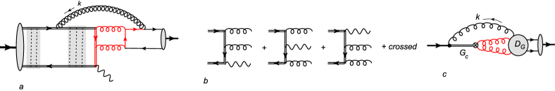
Figure 7: The diagrams describing the colour-octet mechanism in the vector meson production. $(a)$ An example of the diagram with gluons in the intermediate state. The red lines show the hard and hard-collinear particles in SCET-I($v$). The dotted lines in the grey boxes denote Coulomb gluon exchanges. $(b)$ The diagrams describing the hard matching. $(c)$ The diagram in the effective theory describing the matrix element $G_{V}^{\|}$ in Eq.(B.29) .

The hard subprocess describes the annihilation of a heavy quark-antiquark pair into a photon and two hard-collinear gluons in an octet state; see Fig.7$(b)$. Performing the hard factorisation one obtains

$$\left\langle V(p)\right|\epsilon_{\gamma}^{\ast}\cdot J_{Q}(0)\left|\chi_{c1}(P)\right\rangle=i\varepsilon[\epsilon_{\chi},\epsilon_{\gamma}^{\ast},p,q]~{}(\epsilon_{V}^{\ast}\cdot\omega)\frac{m_{V}}{M_{1}^{2}}~{}iA_{Q}^{\|},$$ (B.27)

$$~{}iA_{Q}^{\|}~{}=ee_{Q}~{}\frac{\pi\alpha_{s}(\mu_{h})}{2m^{4}}\int_{0}^{1}d\tau~{}\frac{1}{\tau\bar{\tau}}G_{V}^{\|}(\tau),$$ (B.28)

where $\tau$ is the collinear fraction of the gluon momenta and the function $G_{V}^{\|}(\tau)$ is defined as the matrix element of the following colour-octet operator

$$i\varepsilon[\epsilon_{\chi},\epsilon_{\gamma}^{\ast},p,q]~{}(\epsilon_{V}^{\ast}\cdot\omega)\frac{m_{V}}{M_{1}^{2}}G_{\|}^{V}(\tau)=$$

$$p_{-}\int\frac{d\lambda}{\pi}e^{-i\lambda p_{-}(2\tau-1)}~{}\epsilon_{\gamma}^{\sigma\ast}~{}\left\langle V(p)\right|T\left\{O_{8}^{\sigma}(^{3}S_{1})d^{abc}G_{\bar{n}}^{a\mu}(\lambda\bar{n})G_{\bar{n}\mu}^{b}(-\lambda\bar{n})\right\}\left|\chi_{c1}(P)\right\rangle,$$ (B.29)

where $p_{-}\equiv(p\bar{n})$ and for simplicity, we do not show the Wilson lines in the hard-collinear gluon operator ( $G_{\mu\nu}$ is the gluon strength tensor), using the notation of Eq.(A.9). In the Coulomb limit this matrix element can be computed in the similar way as it was discussed above; see Fig.7$(c)$. We will not repeat the details and provide the complete analytical expression (up to irrelevant constants)

$$\left\langle V(p)\right|\epsilon_{\gamma}^{\ast}\cdot J_{Q}(0)\left|P\right\rangle\sim\left(\epsilon_{V}^{\ast}\cdot\bar{n}\right)~{}ee_{Q}\sqrt{M}\frac{~{}f_{V}m_{V}}{m^{5}}\alpha_{s}(\mu_{h})\alpha_{s}(\mu_{hc})\alpha_{s}(\mu_{us})$$ (B.30)

$$\times\int dx\phi_{\|}^{V}(x)\int_{0}^{1}\frac{d\tau}{\tau\bar{\tau}}\int\frac{d^{3}\mathbf{\Delta}}{(2\pi)^{3}}~{}R_{21}(|\mathbf{\Delta}|)||\mathbf{\Delta}|\int\frac{d^{4}k}{(2\pi)^{4}}D_{G}^{\alpha}(k)\frac{i\varepsilon[\omega\epsilon_{\chi}\lambda\epsilon_{\gamma}^{\ast}]\left\{\omega_{\alpha}k_{\top}^{\lambda}-(g_{\top})_{\alpha}^{\lambda}(\omega k)\right\}}{\left[k^{2}\right]\left[E+(k\omega)+\Delta_{\top}^{2}/m+i\varepsilon\right]^{2}},$$ (B.31)

where the subdiagram $D_{G}$ describes the gluon loop and interaction of the ultrasoft gluon with collinear quarks. The corresponding expression reads

$$D_{G}^{\alpha}(k)=\int d^{D}l\frac{V_{gg}^{\beta\sigma}(l)\text{Tr}\left[\mathcal{P}_{V}\Sigma_{q}^{\alpha\beta\sigma}\right]}{\left[l^{2}\right][(p+k-l)^{2}]},$$ (B.32)

with the gluon operator vertex

$$V_{gg}^{\beta\sigma}\simeq\left\{l_{-}(p_{-}-l_{-})g_{\bot}^{\beta\sigma}-(p_{-}-l_{-})l_{\bot}^{\sigma}\bar{n}^{\beta}+l_{-}l_{\bot}^{\beta}\bar{n}^{\sigma}+l_{\bot}^{2}\bar{n}^{\beta}\bar{n}^{\sigma}\right\}\delta(l_{-}/p_{-}-\tau).$$ (B.33)

In the expression for the light quark part Tr$\left[\mathcal{P}_{V}\Sigma_{q}\right]$ we are projecting the outgoing quark-antiquark pair to the twist-2 collinear operator which yields the meson DA $\phi_{\|}^{V}(x)$, and we expand the resulting QCD expression with respect to small $v$-ultrasoft momentum $k$. For the hard-collinear gluon loop momentum $l$ we assume

$$l_{-}\sim v^{0},~{}\ l_{+}\sim v^{2},~{}l_{\bot}\sim v.$$ (B.34)

The analytical expression for $\Sigma_{q}$ can be obtained from the corresponding QCD diagrams by expansion with respect to ultrasoft momentum $k$, see Fig.8.

Figure 8: The light quark subdiagrams describing the function $\Sigma_{q}$ in Eq.(B.32).

One obtains that the leading-order term scales as

$$V_{gg}^{\beta\sigma}(l)\text{Tr}\left[\mathcal{P}_{V}\Sigma_{q}^{\alpha\beta\sigma}\right]\sim v^{0}.$$ (B.35)

Performing an expansion with respect to $k$ one finds that individual diagrams have the terms of order $v^{-2}$ which appear from the graphs where the ultrasoft photon is attached to the external quark lines. However such contributions cancel because of colour neutrality of the outgoing quark-antiquark pair. This means that the interaction of the ultrasoft gluon with hard-collinear quarks is described by the subleading interactions in the SCET-I($v$) Lagrangian. The analytical result for to the trace in Eq.(B.35) is somewhat lengthy and we will not write it here. Using the estimate (B.35) one finds that

$$D_{G}(k)\sim v^{0},$$ (B.36)

and using this in Eq.(B.30) one obtains

$$\left\langle V(p)\right|\epsilon_{\gamma}^{\ast}\cdot J_{Q}(0)\left|P\right\rangle\sim A_{Q}^{\|}\sim\alpha_{s}(\mu_{h})\alpha_{s}(\mu_{hc})\alpha_{s}(\mu_{us})~{}\lambda^{2}v^{6}\text{.}$$ (B.37)

This estimate is only suppressed by the hard-collinear coupling $\alpha_{s}(\mu_{hc})$ compared to the estimate of the colour-octet amplitudes in Eqs. (B.18) and (B.26). Taking into account that the hard-collinear scale $\mu_{hc}\sim mv$ we obtain $\alpha_{s}(\mu_{hc})\sim v$ . Therefore

$$A_{Q}^{\|}\sim\alpha_{s}(\mu_{h})\alpha_{s}(\mu_{us})~{}\lambda^{2}v^{7}.$$ (B.38)

We next discuss the colour-octet contribution in the amplitude with a transverse meson. In this case we consider the diagram as in Fig.6 projecting the two-quark state to the twist-3 DA. In the general case one has to consider two- and three-point matrix elements which depend on all possible DAs. For simplicity we only consider the two-point matrix elements and pick up the so-called Wandzura-Wilzcek contribution which is completely determined by the leading twist DA $\phi_{\|}^{V}$. The description of the corresponding matrix element and corresponding twist-3 DAs can be found in Appendix A. The heavy quark part in this case is the same as in Eq.(B.11); therefore we can write

$$~{}i\varepsilon[\epsilon_{V}^{\ast},\epsilon_{\gamma}^{\ast},p,q]~{}(\epsilon_{\chi}\cdot q)\frac{1}{M^{2}_{1}}\left[A_{V}^{\bot}\right]_{oct}\sim~{}\frac{f_{V}~{}m_{V}}{m^{3}}\alpha_{s}(\mu_{h})\alpha_{s}(\mu_{us})\sqrt{M}$$

$$\times\int\frac{d^{3}\mathbf{\Delta}}{(2\pi)^{3}}|\boldsymbol{\Delta}|\tilde{R}_{21}(|\mathbf{\Delta}|)\int_{0}^{1}dx~{}\int d^{4}k~{}\frac{\text{Tr}[\mathcal{P}_{V}^{tw3}D^{\alpha\beta}_{q}]}{\left[k^{2}\right]}\frac{i\varepsilon[\omega\epsilon_{\chi}\sigma\beta]g\left\{\omega_{\alpha}k_{\top}^{\sigma}-(g_{\top})_{\alpha}^{\sigma}(\omega k)\right\}}{\left[E+(k\omega)+\Delta_{\top}^{2}/m+i\varepsilon\right]^{2}},$$ (B.39)

where the integral over $dx$ denotes the integral over the collinear fraction of the outgoing quarks. The twist-3 projector reads

$$\text{Tr}[\mathcal{P}_{V}^{tw3}D^{\alpha\beta}_{q}]=\left\{g_{V}^{v}(x)(\varepsilon_{V}^{*})_{\sigma\bot}+\int_{0}^{x}du\left[g_{V}^{v}(u)-\phi_{V}^{\|}(u)\right]p_{\sigma}(\varepsilon_{V}^{*})_{\bot}^{\rho}\frac{\partial}{\partial p_{\bot}^{\rho}}\right\}\frac{1}{4}\text{Tr}\left[\gamma^{\sigma}D^{\alpha\beta}_{q}\right]$$

$$-\frac{1}{4}g^{a\,\prime}_{V}(x)\frac{1}{8}\text{Tr}\left[\gamma_{5}\gamma^{\sigma}\hbox to0.0pt{\hbox to5.00002pt{\hfil$\varepsilon$\hfil}\hss}/_{V}^{*}\hbox to0.0pt{\hbox to6.00235pt{\hfil/\hfil}\hss}n\hbox to0.0pt{\hbox to5.00002pt{\hfil$\bar{n}$\hfil}\hss}/\right]\left.\frac{1}{4}\text{Tr}\left[\gamma^{\sigma}\gamma_{5}D^{\alpha\beta}_{q}\right]\right|_{p_{\perp}=0},$$ (B.40)

where $g^{a\,\prime}_{V}(x)=dg^{a}_{V}(x)/dx$. The expression for $D_{q}$ is given in Eq.(36) but external quark momenta $p_{1,2}$ now have transverse components

$$p_{1}=x_{1}p+p_{\bot},~{}p_{2}=x_{2}p-p_{\bot}.$$ (B.41)

The explicit expressions for twist-3 DAs $g^{v}_{V}$ and $g_{V}^{a}$ are given in Eqs.(A.13) and (A.14). Computing the trace and expanding with respect to small $k$ one obtains

$$\frac{1}{4}\text{Tr}[\mathcal{P}_{V}^{tw3}D^{\alpha\beta}_{q}]\simeq\frac{1}{4}\frac{\text{Tr}\left[\not\epsilon_{V}^{\ast}\gamma_{\bot}^{\alpha}\gamma_{\bot}^{\beta}\not\epsilon_{\gamma}^{\ast}\right]}{\left[-2(pk)\right]}\left\{\frac{1}{2\bar{x}^{2}}\int_{x}^{1}dv\frac{\phi(v)}{v}-\frac{1}{\bar{x}}\frac{1}{4}g_{V}^{a\,\prime}(x)+(x\rightarrow\bar{x})\right\}.$$ (B.42)

The dominant contribution arises from the diagrams with soft gluon emission from external quark lines. For the twist-3 case such contributions do not cancel because of the off-shellness of the external particles. Substituting (B.42) into Eq.(B.39) gives

$$\left[A_{1V}^{\bot}\right]_{oct}\sim\frac{f_{V}m_{V}M^{2}_{1}}{m^{7}}\alpha_{s}(\mu_{h})\alpha_{s}(\mu_{us})\sqrt{M_{1}}\int_{0}^{1}dx~{}\left\{\frac{1}{2\bar{x}^{2}}\int_{x}^{1}dv\frac{\phi(v)}{v}-\frac{1}{\bar{x}}\frac{1}{4}g_{V}^{a\,\prime}(x)+(x\rightarrow\bar{x})\right\}$$

$$\times\int\frac{d^{3}\mathbf{\Delta}}{(2\pi)^{3}}|\boldsymbol{\Delta}|\tilde{R}_{21}(|\mathbf{\Delta}|)\int d^{4}k~{}\frac{(\omega k)}{\left[k^{2}\right][-(kn)]\left[E+(k\omega)+\Delta_{\top}^{2}/m+i\varepsilon\right]^{2}}.$$ (B.43)

From this expression one finds the following estimate

$$\left[A_{1V}^{\bot}\right]_{oct}\sim\alpha_{s}(\mu_{h})\alpha_{s}(\mu_{us})\lambda^{4}v^{4}.$$ (B.44)

Let us also note that the collinear integrals in Eq.(B.43) have the endpoint singularities that can be easily seen using an explicit expression for the functions $g^{a,v}_{V}$. Therefore in this case one also has to include endpoint contributions which will not be considered here.

References

- [1] J. V. Bennett et al. [CLEO Collaboration], Phys. Rev. Lett. 101 (2008) 151801 [arXiv:0807.3718 [hep-ex]].
- [2] M. Ablikim et al. [BESIII Collaboration], Phys. Rev. D 83 (2011) 112005 [arXiv:1103.5564 [hep-ex]].
- [3] Y. J. Gao, Y. J. Zhang and K. T. Chao, Chin. Phys. Lett. 23 (2006) 2376 [hep-ph/0607278].
- [4] Y. J. Gao, Y. J. Zhang and K. T. Chao, hep-ph/0701009.
- [5] D. Y. Chen, Y. B. Dong and X. Liu, Eur. Phys. J. C 70 (2010) 177 [arXiv:1005.0066 [hep-ph]].
- [6] C. Patrignani et al. [Particle Data Group], Chin. Phys. C 40 (2016) no.10, 100001.
- [7] N. Brambilla et al. [Quarkonium Working Group Collaboration], hep-ph/0412158.
- [8] J. Bolz, P. Kroll and G. A. Schuler, Phys. Lett. B 392 (1997) 198 [hep-ph/9610265].
- [9] J. Bolz, P. Kroll and G. A. Schuler, Eur. Phys. J. C 2 (1998) 705 [hep-ph/9704378].
- [10] M. Beneke and L. Vernazza, Nucl. Phys. B 811 (2009) 155 [arXiv:0810.3575 [hep-ph]].
- [11] G. P. Lepage, L. Magnea, C. Nakhleh, U. Magnea and K. Hornbostel, Phys. Rev. D 46 (1992) 4052 [hep-lat/9205007].
- [12] G. T. Bodwin, E. Braaten and G. P. Lepage, Phys. Rev. D 51 (1995) 1125 [Phys. Rev. D 55 (1997) 5853] [hep-ph/9407339].
- [13] N. Brambilla, A. Pineda, J. Soto and A. Vairo, Rev. Mod. Phys. 77 (2005) 1423 [hep-ph/0410047].
- [14] C. W. Bauer, S. Fleming and M. E. Luke, Phys. Rev. D 63, 014006 (2000).
- [15] C. W. Bauer, S. Fleming, D. Pirjol and I. W. Stewart, Phys. Rev. D 63, 114020 (2001).
- [16] C. W. Bauer and I. W. Stewart, Phys. Lett. B 516, 134 (2001).
- [17] C. W. Bauer, D. Pirjol and I. W. Stewart, Phys. Rev. D 65, 054022 (2002).
- [18] M. Beneke, A. P. Chapovsky, M. Diehl and T. Feldmann, Nucl. Phys. B 643, 431 (2002).
- [19] M. Beneke and T. Feldmann, Phys. Lett. B 553, 267 (2003).
- [20] E. J. Eichten and C. Quigg, Phys. Rev. D 52 (1995) 1726 [hep-ph/9503356].
- [21] P. Ball and V. M. Braun, Phys. Rev. D 54 (1996) 2182 [hep-ph/9602323].
- [22] P. Ball, V. M. Braun, Y. Koike and K. Tanaka, Nucl. Phys. B 529 (1998) 323 [hep-ph/9802299].
- [23] P. Ball and V. M. Braun, Nucl. Phys. B 543 (1999) 201 [hep-ph/9810475].
- [24] P. Ball, V. M. Braun and A. Lenz, JHEP 0708 (2007) 090 [arXiv:0707.1201 [hep-ph]].
- [25] V. M. Braun, A. N. Manashov and B. Pirnay, Phys. Rev. D 80 (2009) 114002 Erratum: [Phys. Rev. D 86 (2012) 119902] [arXiv:0909.3410 [hep-ph]].
- [26] A. Pineda and J. Soto, Nucl. Phys. Proc. Suppl. 64 (1998) 428 [hep-ph/9707481].
- [27] A. Pineda and J. Soto, Phys. Lett. B 420 (1998) 391 [hep-ph/9711292].
- [28] M. Beneke and V. A. Smirnov, Nucl. Phys. B 522 (1998) 321 [hep-ph/9711391].
- [29] N. Brambilla, A. Pineda, J. Soto and A. Vairo, Phys. Rev. D 60 (1999) 091502 [hep-ph/9903355].
- [30] N. Brambilla, A. Pineda, J. Soto and A. Vairo, Nucl. Phys. B 566 (2000) 275 [hep-ph/9907240].
- [31] V. A. Smirnov, Springer Tracts Mod. Phys. 177 (2002) 1.
- [32] N. Brambilla, P. Pietrulewicz and A. Vairo, Phys. Rev. D 85 (2012) 094005 [arXiv:1203.3020 [hep-ph]].