Parallaxes and Infrared Photometry of three Y0 dwarfs

Abstract

We have followed up the three Y0 dwarfs WISEPA J041022.71+150248.5, WISEPA J173835.53+273258.9 and WISEPC J205628.90+145953.3 using the UKIRT/WFCAM telescope/instruments. We find parallaxes that are more consistent and accurate than previously published values. We estimate absolute magnitudes in photometric pass-bands from $Y$ to $W3$ and find them to be consistent between the three Y0 dwarfs indicating the inherent cosmic absolute magnitude spread of these objects is small. We examine the MKO $J$ magnitudes over the four year time line and find small but significant monotonic variations. Finally we estimate physical parameters from a comparison of spectra and parallax to equilibrium and non-equilibrium models finding values consistent with solar metallicity, an effective temperature of 450-475 K and log g of 4.0-4.5.

1 Introduction

Y dwarfs represent the coolest collapsed objects outside the solar system known to date. They exhibit strong methane absorption where the Wide-field Infrared Survey Explorer mission (WISE; Wright et al. 2010) $W1$ 3.4 $\mu$m filter is centered and emit about half their energy in the WISE $W2$ 4.6 $\mu$m pass band (Mainzer et al. 2011). This makes the $W1-W2$ color very distinct for these objects and most of the known Y dwarfs have been discovered following their identification as colour-selected candidates in the WISE data (e.g. Cushing et al. 2011).

The temperatures of the Y0 subclass dwarfs are believed to be around 400 K and their masses to be between 5-30 $M_{Jup}$ (Cushing et al. 2011), overlapping in physical parameter space with many exoplanets, so they can be used as surrogates to understand the atmospheric processes of exoplanets. The older examples will hold the chemical imprint of the early Galaxy and the distribution in age may help map out the evolution of formation mechanisms over the Galaxy’s lifetime.

In this contribution we discuss the three objects WISEPA J041022.71+150248.5, WISEPA J173835.53+273258.9 and WISEPC J205628.90+145953.3 which will refer to as 0410, 1738 and 2056 respectively. These were all originally presented in Cushing et al. (2011) and classified as spectral types Y0. First we discuss the astrometry, then the photometry and finally we combine these observations with published spectra and models to estimate physical parameters.

2 Astrometric Analysis

Table 1: Parallaxes and proper motions for UKIRT Y0 targets.

Short	RA,         Dec	Epoch	Absolute $\pi$	$\mu_{\alpha}$	$\mu_{\delta}$	COR	$N_{*},N_{e}$	$\Delta$T	$V_{tan}$
Name	(h:m:s),   (∘:’:”)	(yr)	(mas)	(mas/yr)	(mas/yr)	(mas)		(yr)	(km/s)
0410	4:10:23.0, +15:02:37.8	2014.9551	144.3 $\pm$ 9.9	956.8 $\pm$ 5.6	-2221.2 $\pm$ 5.5	0.97	99, 19	4.36	79.4 $\pm$ 5.4
1738	17:38:35.6, +27:32:57.8	2013.2584	128.5 $\pm$ 6.3	345.0 $\pm$ 5.7	-340.1 $\pm$ 5.1	0.63	293, 18	4.53	17.9 $\pm$ 0.9
2056	20:56:29.0, +14:59:54.6	2012.8274	148.9 $\pm$ 8.2	826.4 $\pm$ 5.5	530.7 $\pm$ 8.5	0.67	452, 18	4.54	31.3 $\pm$ 1.7

COR = correction to absolute parallax, $N_{*}$ = number of reference stars, $N_{e}$ = number of epochs, $\Delta$T = epoch range, $V_{tan}$= tangential velocity.

2.1 Observational Data

The astrometric observations were all made on the UKIRT 3.8 m telescope using the WFCAM imager, which was the combination used to produce the UKIDSS surveys (e.g. Warren et al. 2007). All observations are carried out in queue override mode, allowing us to be very flexible in the scheduling, maximising the parallax factor and observing close to meridian passage. The first observations of these objects were made in September 2011 following a Director Discretionary Time request (U/11B/D1). During the 2012A semester they were included as part of the UKIRT ultra cool dwarf parallax program described in Smart et al. (2010) and Marocco et al. (2010, hereafter MSJ10). In 2014 via a request to the University of Arizona (U/14B/UA15) we obtained further observations. The results published here are based on observations from September 2011 to April 2016. The basic procedures for observing, image treatment and parallax determination follow those described in MSJ10.

One of the most important aspects in the determination of small field parallaxes is stability of the focal plane and repetition of the observational procedure. This is particularly true for the large off axis detectors of the WFCAM instrument. In the MSJ10 program we required that the targets are observed in the same physical position on the focal plane as the discovery image in the UKIDSS survey. As these Y0 dwarfs were not in the UKIDSS survey we had the ability to place the target on any of the 4 chips. For 1738 and 2056 they were placed in the most central quadrant - with respect to the optical axis - of chip 3. This region being close to the optical axis is astrometrically “quiet”. For 0410, in an attempt to also include the T6 dwarf WISEP J041054.48+141131.6 in chip 1, we placed it in the top outside quadrant of chip 4. Unfortunately the T6 is not in the chip 1 as we hoped, but once the first image was taken we kept the same relative position.

For each target we only used reference stars within a limited radius. The size of the radius is a compromise between limiting the number of reference stars and having a large astrometrically complex area to transform. For all targets we choose 2 arcminutes which provided over 50 reference stars. There is a factor of 4 difference between the number of reference stars for 2056 vs 0410 (see $N_{*}$ in Table 1) but 50 was still considered sufficient to astrometrically model such a small area.

As these objects are fainter in the $J$ band than the other targets in the MSJ10 program we increased the exposure time following a 5 jitter (dithered) 3.2” cross pattern, and at each jitter position we made 4 exposures in 2$\times$2 micro-stepped positions of 1.5 pixels, where each exposure consists of 4 co-added 10 second images. The total exposure time is therefore $5\times 4\times 4\times 10=800$ seconds. In average conditions this provides a signal-to-noise of 50 at MKO $J=19.5$.

All observations are reduced using the standard WFCAM Cambridge Astronomical Survey Unit (CASU) pipeline. We transformed all frames to a base frame using a simple six constant linear astrometric fit. We then removed any frames that have an average reference star error larger than the mean error for all frames plus three standard deviations about that mean in either coordinate, or, have less than 12 stars in common with the base frame. Each observation has a quoted positional error from the UKIRT pipeline based the profile fitting program, and the errors in the transformation parameters. However, there remains a systematic contribution to the error that changes from night to night. For this reason, when fitting for the astrometric parameters to the individual observations on the combined frames we treat each observation with equal weight and then calculated the final error on the target parameters from the co-variance matrix of the solution scaled by the error of unit weight. This fit is also iterated removing any observations where the combined residual in the two coordinates is greater than three times the sigma of the whole solution.

The solutions were tested for robustness using bootstrap-like testing where we iterate through the sequence selecting different frames as the base frame thus making many solutions that incorporate slightly different sets of reference stars and starting from different dates. We select all solutions with: (i) a parallax within one sigma of the median solution; (ii) the number of included observations in the top 10%, and (iii) at least 20 reference stars in common to all frames. From this subset, for this publication, we have selected the one with the smallest error. More than 90% of the solutions are within one sigma of the published solution.

To these relative parallaxes we add a correction (COR in Table 1) to find the astrophysically useful absolute parallaxes. The COR is estimated from the average magnitude of the reference stars and the model of Mendez & van Altena (1996) transformed into the J band.

Figure 1: Observations and solution for 0410, 1738 and 2056 from top to bottom panels respectively. The base frame selected is indicated by a circle and any observations rejected are indicated by X. The error bars are the formal centroiding errors from the CASU pipeline in both coordinates.

2.2 Astrometric Parameters

In Table 1 we report the derived absolute parallaxes, proper motions and details of the solutions for the UKIRT sequences. In Fig. 1 we plot the observations and the predicted movement of the targets from our parameters. The result for 0410 is lower precision than 1738 and 2056 probably due to the higher proper motion, since any error in our estimation of this motion will propagate into the parallax estimate.

2.3 Comparison to published values

Parallaxes for these objects have been measured by three teams Marsh et al. (2013), Beichman et al. (2014), and Dupuy & Kraus (2013, hereafter D&K13). The Marsh et al. and and Beichman et al. works used combinations of WISE $W2$, WIRC $J$, NEWFIRM, Spitzer channel 2, and HST $J$ observations with a significant overlap of the two sets of observations. The Marsh results for these targets were based on 7-9 observations while those of Beichman, coming later, were based on 14-16. The results for D&K13 were based on 5 Spitzer channel 1 observations. In Kirkpatrick et al. (2011) they also provide parallactic distances but they were preliminary estimates from the Marsh et al. (2013) work so we have only reported the latter values. Considering all the published targets there are 9 Y0 dwarfs with more than one estimated parallax including the three objects under study here. In Table 2 we have reported all results in common between the three cited works and the results from this contribution.

Table 2: Comparison of parallaxes and proper motions for Y0 dwarfs in different programs.

Short	$\mu_{\alpha}$	$\mu_{\delta}$	Absolute $\pi$	Ref
Name	(mas/yr)	(mas/yr)	(mas)
0254	2588$\pm$27	273$\pm$27	135$\pm$15	2
0254	2578$\pm$42	309$\pm$50	185$\pm$42	3
0410	966$\pm$13	-2218$\pm$13	160$\pm$9	1
0410	958$\pm$37	-2229$\pm$29	132$\pm$15	2
0410	974$\pm$79	-2144$\pm$72	233$\pm$56	3
0410	956$\pm$06	-2223$\pm$6	144$\pm$10	4
1405	-2263$\pm$47	288$\pm$41	129$\pm$19	2
1405	-2297$\pm$96	212$\pm$137	133$\pm$81	3
1541	-857$\pm$12	-087$\pm$13	176$\pm$9	1
1541	-870$\pm$130	-013$\pm$58	74$\pm$31	2
1541	-983$\pm$111	-276$\pm$116	-21$\pm$94	3
1738	317$\pm$09	-321$\pm$11	128$\pm$10	1
1738	292$\pm$63	-396$\pm$22	102$\pm$18	2
1738	348$\pm$71	-354$\pm$55	66$\pm$50	3
1738	346$\pm$6	-338$\pm$5	129$\pm$6	4
1741	-509$\pm$35	-1463$\pm$32	180$\pm$15	2
1741	-495$\pm$11	-1472$\pm$13	176$\pm$26	3
1804	-269$\pm$10	035$\pm$11	80$\pm$10	1
1804	-242$\pm$26	017$\pm$22	60$\pm$11	2
1828	1024$\pm$7	174$\pm$6	106$\pm$7	1
1828	1020$\pm$15	173$\pm$16	70$\pm$14	2
2056	812$\pm$9	534$\pm$8	140$\pm$9	1
2056	761$\pm$46	500$\pm$21	144$\pm$23	2
2056	881$\pm$57	544$\pm$42	144$\pm$44	3
2056	828$\pm$6	532$\pm$8	149$\pm$8	4

References: 1:Beichman et al. (2014), 2:Dupuy & Kraus (2013), 3:Marsh et al. (2013) and 4: this work. Note D&K13 only publish relative parallaxes which is what we have reported here. The targets are 0254: WISE J025409.45+022359.1, 0410: WISEPA J041022.71+150248.5 1405: WISE J140518.40+553421.5, 1541: WISE J154151.65–225025.2, 1738: WISE J173835.52+273258.9, 1741: WISE J174124.26+255319.5, 1804: WISE J180435.40+311706.1, 1828: WISE J182831.08+265037.8, 2056: WISE J205628.90+145953.3.

Figure 2: Parallaxes differences compared to the D&K13 values as multiples of the combined standard deviation for each solution. The D&K13 value is used as the reference as they have published a parallaxes for all of the Y0 dwarfs considered here. References and target abbreviations as in Table 2. So for example the Marsh value of 0254 is one combined sigma larger than the D&K13 value.

In Fig. 2 we plot the differences of the parallax values for the 9 targets with respect to the D&K13 value divided by the error of the two estimates combined in quadrature. The D&K13 values are relative but the difference between relative and absolute parallax is negligible compared to the random errors. The 1541 and 1738 Marsh et al. values are very different from the other values for these targets and are also significantly lower than the predicted spectroscopic parallax so we assume these are compromised. Given the short time baseline and mixed observational sources for the Marsh et al. work it is to be expected that in some solutions the proper motion and parallax were not disentangled correctly. Apart from the two low Marsh et al. values all the other D&K13 estimates appear as underestimates, on average by one combined sigma.

D&K13 publish relative parallaxes not absolute ones because they felt the correction was negligible. The corrections we have applied are less than 1 mas and since the average reference star is fainter in the Spitzer fields we would expect the D&K13 corrections to be even smaller. A correction will reduce the difference in the right direction but we agree with the authors that it cannot be the main cause of the observed difference. We also note in Tinney et al. (2014) they also find the D&K13 parallax estimates are low for other targets. This comparison to the D&K13 values indicates the most reliable results are those of Beichman et al. The difference between the results published here and those of Beichman et al. are all within one sigma. We consider this a confirmation of our procedures, parallax estimates and, importantly, error estimates.

2.4 Search for common proper motion objects and moving group membership

We searched for common proper motion companions to our 3 Y dwarfs within the Hipparcos Main Catalogue, the Gliese Catalogue of Nearby Stars, the Tycho-2 catalogue, and the Fourth U.S. Naval Observatory CCD Astrograph Catalogue. We looked for objects with differences in both proper motion components $<3\sigma$ and a maximum projected separation $<100,000$ AU. The search returned no matches.

We used the BANYAN II online tool (Malo et al. 2013; Gagné et al. 2014) to assess the membership of our targets to nearby moving groups. None of the targets have significant probability of belonging to any of the moving groups. However, for 2056, we obtained a probability of $44\%$ to be a old field member and $56\%$ to be a young field member, suggesting that this object might pertain to a slightly younger population. The tangential velocity, listed in the last column of Table 1, of 0410 is significantly larger than both 1738 and 2056 suggesting it might be old but it does not exceed the $V_{tan}>100$ km s^-1 criteria adopted for ultracool dwarfs belonging to either the Galactic thick disk or halo (Faherty et al. 2009).

We also used LACEwING to access membership assuming the three targets are field objects - e.g. that we have no evidence of youth. Again none of the targets show a significant probability of being in a moving group though 2056 did have a 30% probability of belonging to the Argus group. We conclude that these objects are not members of any know moving groups and are probably just local field members.

3 Photometric Analysis

3.1 Photometric Analysis of WFCAM data

The CASU pipeline estimates the MKO $J$ magnitude of our targets using  100-200 calibrating stars from the Two Micron All Sky Survey (Skrutskie et al. 2006, , hereafter 2MASS) as described in Hodgkin et al. (2009). The systematic errors of the calibration from 2MASS stars is estimated to be better than 1.5% (Hodgkin et al. 2009). The random error is calculated in the pipeline procedures. Following the recommendation in Dye et al. (2006) we have adopted the aperMag3 parameter as the best estimate of the total magnitude for point sources.

In Fig. 3 we plot the variation of the $J$ magnitude for the parallax program observations with respect to the mid-epoch. In Table 3 we report the number of observations, the magnitude, standard deviation, the error of the mean and the slope of the best fit straight line. The long term changes of 0410 and 1738 do appear to be significant, indicating a slow dimming over the period observed, the number of observations is, however, very low and quite noisy. Further observations of these targets are needed to confirm the observed trends.

We adopt the mean magnitude from Table 3 as the best estimate of the MKO magnitude for these targets. To provide a conservative estimate of the error of the mean we simply add 0.02 magnitudes to account for the 1.5% systematic error estimates from Hodgkin et al. (2009).

Table 3: Mean MKO $J$ magnitudes and variations with time.

Target	N	$<J>$	$\sigma$	$\sigma_{mean}$	Slope
		mag	mag	mag	mag/yr
0410	19	19.137	0.103	0.031	-0.044 $\pm$ 0.016
Anon		18.789	0.219	0.054	0.010 $\pm$ 0.038
1738	18	19.539	0.051	0.023	-0.029 $\pm$ 0.010
Anon		19.048	0.068	0.026	-0.004 $\pm$ 0.058
2056	20	19.237	0.062	0.024	0.018 $\pm$ 0.012
Anon		18.593	0.005	0.020	-0.003 $\pm$ 0.005

The “Anon” entry for each target is the straight line fit to the anonymous field star in each sequence. The slope is always smaller and within one sigma zero.

Figure 3: MKO $J$ magnitude variations as a function of time for 0410, 1738 and 2056 respectively. In each plot we have included an anonymous object that is nearby in position and magnitude and plotted it’s magnitude variation offset by -0.4 mag.

3.2 Literature Photometry

There are three published MKO $J$ and $H$ values from Leggett et al. (2015), Schneider et al. (2015) and Kirkpatrick et al. (2012) for these targets as reported in Table 4 along with the estimates found in the last section. The differences are significant, reaching 1 magnitude for the H band of target 0410. The Leggett et al. (2015) values are consistently fainter than all these values and this was discussed in that paper. Since the number of estimates is too small to allow any meaningful statistical tests we simply calculate a weighted mean of all values as reported in Table 4 use this in our further analysis.

Table 4: Published MKO $J$ and $H$ magnitudes and weighted means.

Target	MKO $J$, $\sigma$	MKO $H$,$\sigma$	Source
0410	19.44, 0.03	20.02, 0.05	Leggett et al. 2015
	19.33, 0.02	19.90, 0.04	Schneider et al. 2015
	19.24, 0.05	19.05, 0.09	Kirkpatrick et al. 2012
	19.23, 0.05	…	Mean from Table 3
	19.34, 0.02	19.85, 0.03	Weighted mean
1738	19.63, 0.05	20.24, 0.08	Leggett et al. 2015
	19.55, 0.02	20.25, 0.03	Schneider et al. 2015
	19.51, 0.08	20.39, 0.33	Kirkpatrick et al. 2012
	19.52, 0.03	…	Mean from Table 3
	19.55, 0.02	20.25, 0.03	Weighted mean
2056	19.43, 0.04	19.96, 0.04	Leggett et al. 2015
	19.13, 0.02	19.64, 0.03	Schneider et al. 2015
	19.23, 0.13	19.62, 0.31	Kirkpatrick et al. 2012
	19.23, 0.03	…	Mean from Table 3
	19.20, 0.02	19.75, 0.02	Weighted mean

In Table 5 along with the weighted mean $J$ and $H$ magnitudes we report all published photometry from other bands. From the apparent magnitudes we estimate absolute magnitudes assuming a distance given by the parallax in Table 1. The error on the distance is the largest contributor to the error in the absolute magnitude. In the last line of Table 5 we include a weighted mean absolute magnitude and the error of that mean.

In Fig. 4 we plot the absolute MKO $J$ magnitudes vs MKO $J-$ W2 color for various $>$T7 objects with distances and magnitudes taken from Leggett et al. (2015). The three targets presented here are labelled, as are the other Y0 objects in the sample. The weighted mean absolute $J$ and $W2$ magnitudes, 20.05$\pm$0.07 and 14.84$\pm$0.07, from Table 5 can be directly compared to the median absolute magnitudes based on 11 Y0 dwarfs with measured distances in Tinney et al. (2014) of 20.32$\pm$1.25 and 14.65$\pm$0.35. The difference is large but within 1 sigma and as seen from Fig. 4 while the spread of Y0 dwarfs appears large - the three Y0 dwarfs studied here are however very similar. Despite the systematic differences in parallaxes noted in Section 2.3 the mean absolute magnitudes per spectral type derived by D&K13 (table S3) for the $Y,J,H,K,$ Spitzer channel 1 & 2 bands are consistent at the 1 sigma level with our values.

Table 5: Apparent magnitudes from various sources and mean absolute magnitudes as a function of filter.

Band/$\lambda_{eff}$	$z^{1}$,$\sigma$	MKO $Y^{2}$,$\sigma$	MKO $J^{3}$,$\sigma$	MKO $H^{3}$,$\sigma$	MKO $K^{2}$,$\sigma$	Spitzer ch14,$\sigma$	Spitzer ch24,$\sigma$
Target	9535	10289	12444	16221	21900	35075	44366
0410	22.66, 0.09	19.61, 0.04	19.34, 0.02	19.85, 0.03	19.91, 0.07	16.64, 0.04	14.17, 0.02
1738	22.80, 0.09	19.86, 0.07	19.55, 0.02	20.25, 0.03	20.58, 0.10	17.09, 0.05	14.47, 0.02
2056	23.09, 0.08	19.77, 0.05	19.20, 0.02	19.75, 0.02	20.01, 0.06	16.03, 0.03	13.92, 0.02
$<$M$>$	23.57$\pm$ 0.08	20.45$\pm$ 0.07	20.05$\pm$ 0.07	20.65$\pm$ 0.07	20.86$\pm$ 0.08	17.24$\pm$ 0.07	14.87$\pm$ 0.07
Band/$\lambda_{eff}$	WISE $W1^{4}$,$\sigma$	WISE $W2^{4}$,$\sigma$	WISE $W3^{4},\sigma$	$F125W^{5},\sigma$	$F140W^{5},\sigma$	Distance
Target	33526	46028	115608	12305	13645	Modulus
0410	$>$18.170	14.11, 0.05	12.31, 0.50	20.00, 0.03	19.64, 0.02	$0.80^{+0.14}_{-0.14}$
1738	17.71, 0.16	14.50, 0.04	12.45, 0.40	20.22, 0.02	19.92, 0.02	$0.54^{+0.11}_{-0.10}$
2056	16.48, 0.08	13.84, 0.04	11.73, 0.25	19.81, 0.02	19.48, 0.02	$0.76^{+0.10}_{-0.11}$
$<$M$>$	17.57$\pm$ 0.11	14.84$\pm$ 0.07	12.71$\pm$ 0.21	20.69$\pm$ 0.07	20.37$\pm$ 0.07

References: 1: Lodieu et al. (2013), 2: Leggett et al. (2015), 3: This work, 4: Kirkpatrick et al. (2012) and 5: Schneider et al. (2015). The $\lambda_{eff}$ row is the simple median effective wavelength for a convolution of the nominal filter profile and a Vega spectra, this is often not appropriate for these objects because of the structure in the underlying spectra but it is provided for reference. The published apparent magnitudes are converted to absolute magnitudes using the distance modulus from the parallaxes presented in Table 1. The $<$M$>$ row is the weighted mean absolute magnitude for all three targets along with the error of the mean for each filter.

Figure 4: The absolute MKO $J$ magnitude versus the MKO $J$ - W2 color for published $>$T7 objects from Leggett et al. (2015) along with the objects presented here. The spectral types at the top of the graph are provided just as indicative ranges, the labelled objects are the Y0 dwarfs 0359 WISE J035934.06–540154.6, 0713: WISE J071322.55–291751.9, 0734: WISE J073444.02–715744.0, 1405: WISEP J140518.40+553421.5 and 2220: WISE J222055.31–362817.4. The $<$M$>$ point is the weighted mean absolute magnitude as found in Table 5.

4 Spectroscopic Analysis and Comparison to models

We fit the spectra from Cushing et al. (2011) of our targets with the atmospheric models presented in Tremblin et al. (2015) and Morley et al. (2012); Morley et al. (2014). The Tremblin et al. (2015) model grid covers the $200<T_{\rm eff}<1000$ K range with log g values of 4.0, 4.5, and 4.8. We examined both solar metallicity models as well as metal-poor models with [M/H] = -0.5 – -0.8, and both equilibrium and non-equilibrium models with log $K_{\rm zz}=6$. The Tremblin et al. (2015) models do not take into account clouds. The models from Morley et al. (2012) are computed for $400\leq T_{\rm eff}\leq 1300$ K, log g 4.0, 4.5, 5.0, and 5.5, with $2\leq f_{\rm sed}\leq 5$. The models from Morley et al. (2014) covers the $200\leq T_{\rm eff}\leq 450$ K range, $3.0\leq{\rm log~{}g}\leq 5.0$, and $3\leq f_{\rm sed}\leq 7$. The Morley et al. (2014) models assume a patchy cloud coverage with only $50\%$ of the object being covered by clouds.

The Cushing et al. (2011) spectra cover the wavelength range 1$-$2.4 $\mu$m at a resolution of R $\approx$ 300 for 0410, 1.07$-$1.70 $\mu$m wavelength range at a low resolving power of R $\approx$ 130 for 1738, and 1.143$-$1.375 $\mu$m and 1.431$-$1.808 $\mu$m at a resolution or R $\approx$ 2500 for 2056.

We derived the best-fit parameters by fitting our model grid to the observed spectra using a standard reduced $\chi^{2}$ minimisation. We used two slightly different approaches. One normalizes both target and model spectra at the peak of the J-band (i.e. 1.26 $\mu$m). The other approach makes use of the parallaxes derived here. The Tremblin et al. (2015) models provide flux at 10 pc (assuming a radius of 0.1 R_⊙), which we have re-scaled for the appropriate radius taken from Saumon & Marley (2008). We then scaled the observed spectra to match the absolute MKO J magnitude, calculated using their measured parallax. A similar procedure was applied to the models from Morley et al. (2012) and Morley et al. (2014). To assess the quality of the best-fit parameters we adopted the approach described in Cushing et al. (2011). Briefly, we generate 10,000 “mimic spectra” for each object by adding Gaussian noise to the observed spectra, preserving the signal-to-noise ratio. Then we fit this 10,000 mimics with the atmospheric models to determine their best-fit parameters. We adopt the range of parameters encompassed by the standard deviation of the resulting distribution as our best-fit values.

The results are summarized in Table 6. The differences between the best-fit parameters derived with the two methods and the different models are small, but with the Tremblin et al. (2015) models giving systematically lower log g and higher $T_{\rm eff}$ values than the Morley et al. (2012); Morley et al. (2014) models. The reason for this systematic difference is beyond the scope of this contribution but it is probably due to the use of different opacity tables, e.g. Tremblin et al. (2015) uses molecular line lists for ammonia from Yurchenko & Tennyson (2014) while Morley et al. (2012); Morley et al. (2014) uses those from Yurchenko et al. (2011).

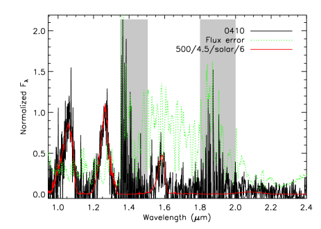
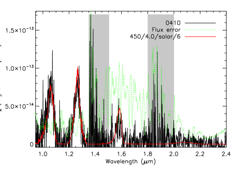
Figure 6: *

Morley et al. (2012) models.

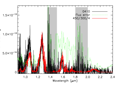
Figure 7: *

Morley et al. (2014) models.

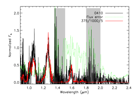
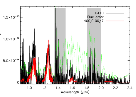
Figure 8: The best-fit model for 0410, obtained normalizing both model and target spectrum in the $J$ band (left panel) or scaling the observed spectrum to match the measured absolute $J$ magnitude (right panel). The spectrum of 0410 is plotted in black, its associated 1 $\sigma$ uncertainty is plotted in green, and the best-fit model is plotted in red. The shaded area are regions which are heavily effected by telluric absorption so are excluded from the model fitting. The best-fit parameters are summarized in the legend, following the scheme $T_{\rm eff}$/log g/[M/H]/log $K_{\rm zz}$ for the Tremblin et al. (2015) models and $T_{\rm eff}$/g/$f_{\rm sed}$ for the Morley et al. (2012) and Morley et al. (2014) models.

For 0410 the best-fit parameters when normalizing the spectra are $T_{\rm eff}\sim 450$ K, log g $\sim$ 4.5, and solar metallicity. The only notable exception are the Morley et al. (2014) models, that would predict a lower $T_{\rm eff}$ of 350$-$400 K. When using the measured parallax we obtain a slightly lower $T_{\rm eff}$. The spectrum of 0410 and the best fit models are plotted in Fig. 8. We note that 500 K is a higher temperature than previously found for Y0s (e.g. Kirkpatrick et al. 2012; Leggett et al. 2013; Beichman et al. 2014), while the value obtained using the parallax is more in line with the published estimates.

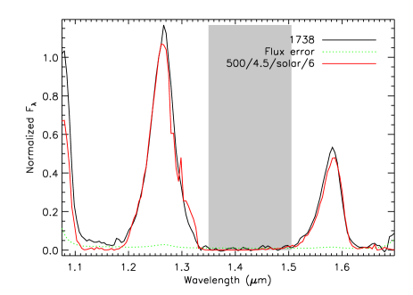
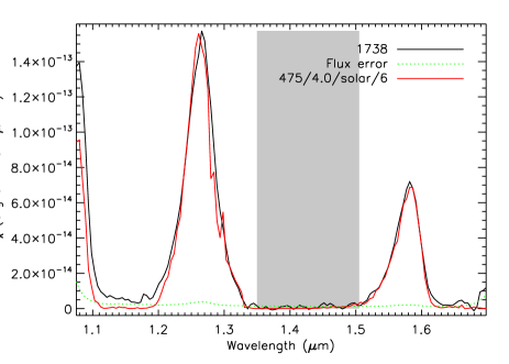
Figure 10: *

Morley et al. (2012) models.

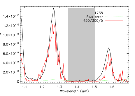
Figure 11: *

Morley et al. (2014) models.

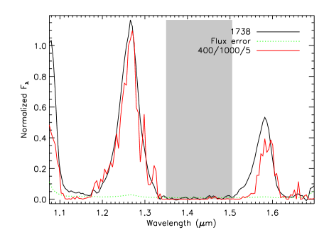
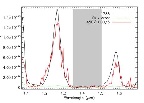
Figure 12: Same as Fig. 8 but for 1738.

For 1738 the best-fit parameters given by the various models tend to be more discordant. When normalizing the spectra the Tremblin et al. (2015) models give $T_{\rm eff}=500$ K and log g $=~{}4.5$ (with solar metallicity and log $K_{\rm zz}=6$). The other models predict a lower $T_{\rm eff}$ of 400 K with a higher log g of $\approx~{}4.75$. Using our measured parallax mitigates the discrepancy, with the Morley et al. (2012); Morley et al. (2014) models returning best-fit $T_{\rm eff}=450$ K and log g $=~{}4.5-5.0$, closer to the Tremblin et al. values. The spectrum of 1738 and the best fit models are plotted in Fig. 12.

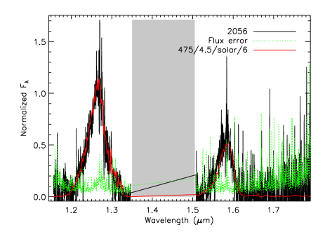
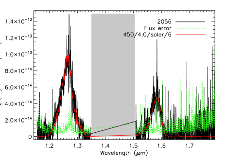
Figure 14: *

Morley et al. (2012) models.

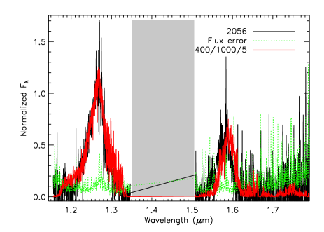
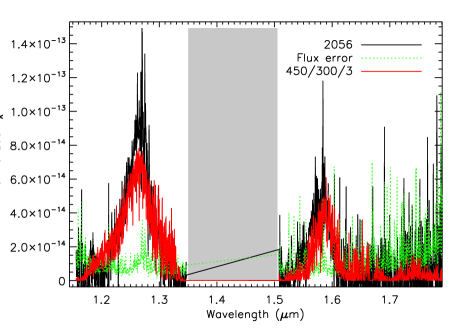
Figure 15: *

Morley et al. (2014) models.

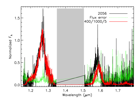
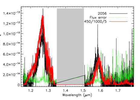
Figure 16: Same as Fig. 8 but for 2056.

For 2056 we have similar situation, with some discrepancy between the best-fit parameters derived from the different models when normalizing the spectra. The Tremblin et al. (2015) models predict slightly higher $T_{\rm eff}$ compared to the other models (450$-$500 K vs. 375$-$450 K), and also in this case the discrepancy is removed when using the measured parallax. The spectrum of 2056 and the best fit models are plotted in Fig. 16.

	This paper									Cushing et al. (2011)
Models	Tremblin et al. (2015)			Morley et al. (2012)			Morley et al. (2014)			Saumon & Marley (2008)
Short	$T_{\rm eff}$	log g	log	$T_{\rm eff}$	log g	$f_{\rm sed}$	$T_{\rm eff}$	log g	$f_{\rm sed}$	$T_{\rm eff}$	log g	log
Name	(K)		$K_{\rm zz}$	(K)			(K)			(K)		$K_{\rm zz}$
0410	500	4.0$-$4.5	6	400$-$450	4.0$-$5.0	4$-$5	350$-$400	4.5$-$5.0	5	450	3.75	0
	450	4.0$-$4.5	6	450	4.0$-$4.5	3$-$5	375$-$400	4.0	5$-$7
1738	475$-$500	4.0$-$4.5	6	400	4.5$-$5.0	4$-$5	400	5.0	5	350	4.75	4
	475	4.0	6	450	4.5	5	450	5.0	5
2056	450$-$500	4.0$-$4.5	6	400$-$450	4.5$-$5.0	4$-$5	375$-$400	5.0	5	350	4.75	4
	450	4.0	6	450	4.5	3$-$4	400$-$450	5.0	5

Table 6: The best-fit parameters obtained with our model fitting, compared with those obtained by Cushing et al. (2011). For each target, the first line presents the parameters obtained normalizing both model and target spectrum in the $J$ band, while the second line presents the parameters obtained scaling the observed spectrum to match the measured absolute $J$ magnitude. The metallicity, [M/H], was a fitted parameter for the Tremblin et al. (2015) models, but always came out to be solar for all sets of parameters.

5 Discussion

We have found parallaxes with relative errors better than 7% using observations from just one telescope and detector combination. The three Y0 objects studied here have absolute magnitudes that are consistent to within the observational errors and we find mean absolute magnitudes for various pass-bands. A comparison to other parallaxes determinations shows our values to be consistent with those of Beichman et al (2014) but indicate the values in Dupuy & Kraus (2013) are underestimated. While Dupuy & Kraus published only relative parallaxes the observed difference is too large to be due to a required correction to an absolute value.

This difference must lie in the reduction procedures or in some systematic bias in the observational material. Parallaxes of objects this faint will remain the domain of relative small field programs for the near future but with wealth of objects being published by Gaia a gold standard will be produced which will allow small field programs to calibrate instruments and refine procedures to the sub-mas level. Also, while Gaia will not observe directly any objects cooler than late T dwarfs it will indirectly detect cool objects in binary systems that will serve as direct comparisons in absolute magnitude space to those measured with small field programs. The ability to detect and remove systematic errors from the observations and reductions along with a direct comparison sample will lead to more robust and consistent small field results that will only aid the astrophysical interpretation.

As shown in Section 3 our multi-epoch observations sample the near-infrared brightness evolution of the three targets over a baseline of about 4 years. Simple linear fits to the $J$ measurements show small and marginally statistically significant long-term slopes in two of our targets and indicate a possible slope in the third target (Table 3). Although the existence of long-term monotonic variations is tentative, this possibility is intriguing and in the following we briefly explore their possible nature.

Our measurements represent the first long-term precision photometry of Y dwarfs and, as such, the first probes of long-term atmospheric evolution in these objects. Recent precision near-infrared (Spitzer) studies of Y-dwarfs detected high-amplitude ($\sim$3%–15%) rotational modulations in three targets: WISEP J140518.40+553421.5 (Cushing et al. 2016); WISE J173835.52+273258.9 (Leggett et al. 2016b) and WISE J085510.83–071442.5 (Esplin et al. 2016). These modulations are periodic on the 6 hour timescales, and consistent with rotational modulation that are found to be common in L, L/T, and T-type brown dwarfs by extensive and sensitive space-based surveys (Buenzli et al. 2014; Metchev et al. 2015). Detailed analysis of photometric variability in L/T dwarfs indicated variations of cloud properties (e.g. Artigau et al. 2009; Radigan et al. 2012), which was verified as correlated temperature and cloud thickness variations by high precision time-resolved spectroscopy (Apai et al. 2013). In contrast, for mid-L type brown dwarfs modulations in the condensate cloud properties failed to reproduce the observed gray variations and indicate a high-level haze layer (Yang et al. 2016). The observed modulations in Y-dwarfs are probably emerging due to the rotational modulations introduced by heterogeneous KCl and Na₂S clouds (Leggett et al. 2016a).

Unlike the above studies, our observations provide a sensitive probe of Y-dwarfs over very long timescales, i.e., over $10^{4}$ rotations. Our data hints on the possible existence of monotonic changes, which is not consistent with stochastic cloud evolution (occurring over dynamical timescales, about a rotational period). Although the full interpretation of the variations is beyond the scope of this work, we embark here on a speculative discussion of the importance of the photometric variations. The changes, if real, are probably occurring due to a long-term monotonic evolution of the clouds, driven by a process that acts on a timescale much longer than the dynamical timescales. We note that chemical disequilibrium could drive such slow changes if the kinetic timescales for one or more important processes are very long. An example of such slow, chemical disequilibrium-driven cloud evolution is given by the spectacular 2012 Saturn Storm (Sromovsky et al. 2013). During this event water vapor-rich air was dredged up from the deep interior of Saturn to its upper, cold and very dry atmosphere. Water and other volatiles froze out in the upper atmosphere and formed clouds that were optically thick at optical and infrared wavelengths. Over the course of the following six months the clouds encompassed Saturn’s northern hemisphere and eventually dispersed, with ice crystals likely settling to the deeper interior, leaving the upper atmosphere dry again. We speculate here that qualitatively similar events may drive long-timescale monotonic brightness evolution in Y-dwarfs.

We have compared the combination of spectra and parallaxes to the atmospheric models of Tremblin et al. (2015) and Morley et al. (2012, 2014). We find the best physical parameters are consistent between the three objects with solar metallicity, temperatures between 450-475 K, and a log g of 4.0-4.5. A general consideration that arises from the model fitting is that, if we do not employ the measured parallax, the models alone would lead to overestimated log g, i.e. we would essentially be overestimating the mass of our targets. We note that for Tremblin et al. (2015) all best fit models are non-equilibrium models, stressing the importance of mixing in such low-temperature atmospheres. All Tremblin et al. (2015) best-fit models are solar-metallicity models, however given our coarse metallicity grid, this result is less conclusive. All Y dwarfs have best-fit log g $\geq$ 4.0, suggestive of “old”, evolved objects (age $>$ 1 Gyr), in agreement with their kinematics. If we compare the parameters derived here with those presented in Cushing et al. (2011), we note that we either get a significantly higher $T_{\rm eff}$ ($\sim 100-150$ K higher, for 1738 and 2056), or a significantly higher log g (0.75 dex, for 0410). While comparing the results from different model grids is a dangerous exercise, (given the disparate underlying assumptions, the different parameter space covered, and the heterogeneous steps of the grid), it is however remarkable to see such a large discrepancy in the predicted atmospheric parameters. Finally, we stress that this analysis is based on near-infrared spectra only, while Y dwarfs emit most of their energy at longer wavelengths. Any systematic issue with models in the near-infrared range would therefore lead to incorrect atmospheric parameters.

Figure 5: *

Tremblin et al. (2015) models.

Figure 9: *

Tremblin et al. (2015) models.

Figure 13: *

Tremblin et al. (2015) models.

6 Acknowledgments

We thank the anonymous referee for comments that improved the clarity of this contribution; Isabelle Baraffe and Gilles Chabrier for useful discussions on the model aspects addressed here; Luca Rizzi, Tom Kerr, Watson Varricatt and Andy Adamson for scheduling help; and Mike Cushing who promptly provided the spectra of these three targets. This work has made use of the Cambridge Astronomy Survey Unit software and the WFCAM Science Archive thanks to Mike Irwin and Mike Read for their support. The United Kingdom Infrared Telescope was operated by the Joint Astronomy Centre on behalf of the Science and Technology Facilities Council of the U.K., it is currently operated by the University of Arizona. RLS’s research was supported by a Henri Chrétien International Research Grant administered by the American Astronomical Society and a Visiting Professorship with the Leverhulme Trust (VP1-2015-063). SKL’s research is supported by the Gemini Observatory, which is operated by the Association of Universities for Research in Astronomy, Inc., on behalf of the international Gemini partnership of Argentina, Australia, Brazil, Canada, Chile and the United States of America. FM/HRAJ/DJP acknowledge support from the UK’s Science and Technology Facilities Council grant number ST/M001008/1. The collaboration was supported by the Marie Curie 7th European Community Framework Programme grant n.247593 Interpretation and Parameterisation of Extremely Red COOL dwarfs (IPERCOOL) International Research Staff Exchange Scheme.

References

- Apai et al. (2013) Apai D., Radigan J., Buenzli E., Burrows A., Reid I. N., Jayawardhana R., 2013, ApJ, 768, 121
- Artigau et al. (2009) Artigau É., Bouchard S., Doyon R., Lafrenière D., 2009, ApJ, 701, 1534
- Beichman et al. (2014) Beichman C., Gelino C. R., Kirkpatrick J. D., Cushing M. C., Dodson-Robinson S., Marley M. S., Morley C. V., Wright E. L., 2014, ApJ, 783, 68
- Buenzli et al. (2014) Buenzli E., Apai D., Radigan J., Reid I. N., Flateau D., 2014, ApJ, 782, 77
- Cushing et al. (2011) Cushing M. C., et al., 2011, ApJ, 743, 50
- Cushing et al. (2016) Cushing M. C., et al., 2016, ApJ, 823, 152
- Dupuy & Kraus (2013) Dupuy T. J., Kraus A. L., 2013, Science, 341, 1492
- Dye et al. (2006) Dye S., et al., 2006, MNRAS, 372, 1227
- Esplin et al. (2016) Esplin T. L., Luhman K. L., Cushing M. C., Hardegree-Ullman K. K., Trucks J. L., Burgasser A. J., Schneider A. C., 2016, ApJ, 832, 58
- Faherty et al. (2009) Faherty J. K., Burgasser A. J., Cruz K. L., Shara M. M., Walter F. M., Gelino C. R., 2009, AJ, 137, 1
- Gagné et al. (2014) Gagné J., Lafrenière D., Doyon R., Malo L., Artigau É., 2014, ApJ, 783, 121
- Hodgkin et al. (2009) Hodgkin S. T., Irwin M. J., Hewett P. C., Warren S. J., 2009, MNRAS, 394, 675
- Kirkpatrick et al. (2011) Kirkpatrick J. D., et al., 2011, ApJS, 197, 19
- Kirkpatrick et al. (2012) Kirkpatrick J. D., et al., 2012, ApJ, 753, 156
- Leggett et al. (2013) Leggett S. K., Morley C. V., Marley M. S., Saumon D., Fortney J. J., Visscher C., 2013, ApJ, 763, 130
- Leggett et al. (2015) Leggett S. K., Morley C. V., Marley M. S., Saumon D., 2015, ApJ, 799, 37
- Leggett et al. (2016a) Leggett S. K., et al., 2016a, preprint, (arXiv:1607.07888)
- Leggett et al. (2016b) Leggett S. K., et al., 2016b, ApJ, 830, 141
- Lodieu et al. (2013) Lodieu N., Béjar V. J. S., Rebolo R., 2013, A&A, 550, L2
- Mainzer et al. (2011) Mainzer A., et al., 2011, ApJ, 726, 30
- Malo et al. (2013) Malo L., Doyon R., Lafrenière D., Artigau É., Gagné J., Baron F., Riedel A., 2013, ApJ, 762, 88
- Marocco et al. (2010) Marocco F., et al., 2010, A&A, 524, A38+
- Marsh et al. (2013) Marsh K. A., Wright E. L., Kirkpatrick J. D., Gelino C. R., Cushing M. C., Griffith R. L., Skrutskie M. F., Eisenhardt P. R., 2013, ApJ, 762, 119
- Mendez & van Altena (1996) Mendez R. A., van Altena W. F., 1996, AJ, 112, 655
- Metchev et al. (2015) Metchev S. A., et al., 2015, ApJ, 799, 154
- Morley et al. (2012) Morley C. V., Fortney J. J., Marley M. S., Visscher C., Saumon D., Leggett S. K., 2012, ApJ, 756, 172
- Morley et al. (2014) Morley C. V., Marley M. S., Fortney J. J., Lupu R., Saumon D., Greene T., Lodders K., 2014, ApJ, 787, 78
- Radigan et al. (2012) Radigan J., Jayawardhana R., Lafrenière D., Artigau É., Marley M., Saumon D., 2012, ApJ, 750, 105
- Saumon & Marley (2008) Saumon D., Marley M. S., 2008, ApJ, 689, 1327
- Schneider et al. (2015) Schneider A. C., et al., 2015, ApJ, 804, 92
- Skrutskie et al. (2006) Skrutskie M. F., et al., 2006, AJ, 131, 1163
- Smart et al. (2010) Smart R. L., et al., 2010, A&A, 511, A30+
- Sromovsky et al. (2013) Sromovsky L. A., Baines K. H., Fry P. M., 2013, Icarus, 226, 402
- Tinney et al. (2014) Tinney C. G., Faherty J. K., Kirkpatrick J. D., Cushing M., Morley C. V., Wright E. L., 2014, ApJ, 796, 39
- Tremblin et al. (2015) Tremblin P., Amundsen D. S., Mourier P., Baraffe I., Chabrier G., Drummond B., Homeier D., Venot O., 2015, ApJ, 804, L17
- Warren et al. (2007) Warren S. J., et al., 2007, MNRAS, 375, 213
- Wright et al. (2010) Wright E. L., et al., 2010, AJ, 140, 1868
- Yang et al. (2016) Yang H., et al., 2016, ApJ, 826, 8
- Yurchenko & Tennyson (2014) Yurchenko S. N., Tennyson J., 2014, MNRAS, 440, 1649
- Yurchenko et al. (2011) Yurchenko S. N., Barber R. J., Tennyson J., 2011, MNRAS, 413, 1828