Exploring the resonances $X(4140)$ and $X(4274)$ through their decay channels

Abstract

Investigation of the resonances $X(4140)$ and $X(4274)$, which were recently confirmed by the LHCb Collaboration Aaij:2016iza , is carried out by treating them as the color triplet and sextet $[cs][\bar{c}\bar{s}]$ diquark-antidiquark states with the spin-parity $J^{P}=1^{+}$, respectively. We calculate the masses and meson-current couplings of these tetraquarks in the context of QCD two-point sum rule method by taking into account the quark, gluon and mixed vacuum condensates up to eight dimensions. We also study the vertices $X(4140)J/\psi\phi$ and $X(4274)J/\psi\phi$, and evaluate corresponding strong couplings $g_{X(4140)J/\psi\phi}$ and $g_{X(4274)J/\psi\phi}$ by means of QCD light-cone sum rule method, and a technique of the soft-meson approximation. In turn, these couplings contain a required information to determine the width of the $X(4140)\to J/\psi\phi$ and $X(4274)\to J/\psi\phi$ decay channels. We compare our results for the masses and decay widths of the $X(4140)$ and $X(4274)$ resonances with the LHCb data, and alternative theoretical predictions.

I Introduction

Recently the LHCb Collaboration presented results of analysis of the exclusive decays $B^{+}\rightarrow J/\psi\phi K^{+}$, and confirmed existence of the resonances $X(4140)$ and $X(4274)$ in the $J/\psi\phi$ invariant mass distribution Aaij:2016iza . It also reported on observation of the heavy resonances $X(4500)$ and $X(4700)$ in the same $J/\psi\phi$ channel. The measured masses and decay widths of these resonances (hereafter $X(4140)\Rightarrow X_{1},\ X(4274)\Rightarrow X_{2},\ X(4500)\Rightarrow X_{3}$ and $X(4700)\Rightarrow X_{4}$, respectively ) read

$$X_{1}:M=4146\pm 4.5_{-2.8}^{+4.6}\ \mathrm{MeV},\ \Gamma=83\pm 21_{-14}^{+21}\ \mathrm{MeV},$$

$$X_{2}:M=4273\pm 8.3_{-3.6}^{+17.2}\ \mathrm{MeV},\ \Gamma=56\pm 11_{-11}^{+8}\ \mathrm{MeV},$$

$$X_{3}:M=4506\pm 11_{-15}^{+12}\ \mathrm{MeV},\ \Gamma=92\pm 21_{-20}^{+21}\ \mathrm{MeV},$$

$$X_{4}:M=4704\pm 10_{-24}^{+14}\ \mathrm{MeV},\ \Gamma=120\pm 31_{-33}^{+42}\ \mathrm{MeV}.$$

The LHCb determined the spin-parities of these resonances, as well. It turned out, that $X_{1}$ and $X_{2}$ are axial-vector states with $J^{PC}=1^{++}$, whereas the quantum numbers of $X_{3}$ and $X_{4}$ are $J^{PC}=0^{++}$.

The resonances $X_{1}$ and $X_{2}$ are old members of the XYZ family of exotic states: They were observed by the CDF Collaboration Aaltonen:2009tz in the decay processes $B^{\pm}\rightarrow J/\psi\phi K^{\pm}$, and later confirmed by CMS Chatrchyan:2013dma and D0 collaborations Abazov:2013xda , respectively. The states $X_{3}$ and $X_{4}$ are heavier than $X_{1},\,X_{2}$, and were found for the first time. All of the $X$ resonances may belong to a class of the hidden-charm exotic states. From production mechanisms and decay channels, it is clear that as tetraquark candidates they should contain strange quark-antiquark pair $s\bar{s}$. In other words, the quark content of the $X$ states is $c\bar{c}s\bar{s}$.

The unconventional hadrons, such as glueballs, hybrid resonances, exotic four-quark systems and pentaquarks already attracted interests of physicists GellMann:1964nj ; Jaffe:1977 ; Witten:1979kh ; Balitsky:1982ps ; Reinders:1985 ; Braun:1985ah ; Braun:1988kv ; Jaffe:2004zg . Besides general theoretical problems of the multi-parton states, in some of these works their parameters were calculated, as well. The $X$ resonances as the four-quark states can be treated within the diquark-antidiquark Jaffe:2004ph ; Maiani:2004vq or molecular pictures suggested to explain their internal organization. In fact, in theoretical investigations of $X_{1}$ and $X_{2}$ both of these models were used: The resonances $X_{1}$ and $X_{2}$ were considered as the meson molecules in Refs. Liu:2008tn ; Wang:2009ue ; Albuquerque:2009ak ; Wang:2009ry ; Wang:2011uk ; Liu:2010hf ; He:2011ed ; Finazzo:2011he ; HidalgoDuque:2012pq , whereas in Ref. Stancu:2009ka ; Patel:2014vua they were treated in the framework of the diquark-antidiquark model. There are also alternative approaches analyzing them as dynamically generated resonances Molina:2009ct ; Branz:2010rj or coupled-channel effects Danilkin:2009hr . The recent comprehensive review of the various theoretical models, achieved progress and existing problems in the physics of multiquark resonances can be found in Ref. Esposito:2016noz .

The experimental situation, stabilized after the LHCb report, imposes new constraints on possible models of $X$ resonances. Indeed, an analysis carried out by the LHCb Collaboration in Ref. Aaij:2016iza on the basis of the collected experimental information ruled out an explanation of the $X_{1}$ as $0^{++}$ or $2^{++}$ $D_{s}^{\ast+}D_{s}^{\ast-}$ molecular states. The LHCb also emphasized that molecular bound-states or cusps can not account for $X_{2}$.

Therefore, in order to explain the experimental data, new models and ideas are suggested. First of all, there are traditional attempts to describe the $X$ resonances as excited states of the conventional charmonium or as dynamical effects. Indeed, by analyzing experimental information of the Belle and BaBar collaborations (see, Refs. Bhardwaj:2015rju and Aubert:2008bl ) on the $B\rightarrow K\chi_{c1}\pi^{+}\pi^{-}$ and $B\rightarrow KD\overline{D}$ decays, in Ref. Chen:2016iua the author identified the resonances $X_{1}$ and $Y(4080)$ with the P-wave excited charmonium states $\chi_{c1}(3^{3}P_{1})$ and $\chi_{c0}(3^{3}P_{0})$, respectively,

The contribution of the rescattering effects to the process $B^{+}\rightarrow J/\psi\phi K^{+}$ was studied in Ref. Liu:2016onn aiming to answer a question can they simulate the observed $X_{1}$, $X_{2}$, $X_{3}$ and $X_{4}$ resonances or not. It was found that the $D_{s}^{\ast+}D_{s}^{-}$ and $\psi^{\prime}\phi$ rescatterings via meson loops may simulate the structures $X_{1}$ and $X_{4}$, respectively. But, description of the $X_{2}$ and $X_{3}$ states as rescattering effects seem are problematic, which implies that they could be real four-quark resonances. Nevertheless, on the basis of some other arguments (see, for details Ref. Liu:2016onn ) the author did not exclude treating of $X_{2}$ as the excited $\chi_{c1}(3^{3}P_{1})$ state of the conventional charmonium.

The diquark-antidiquark and molecule-like models prevail other pictures and form a theoretical basis for numerous calculations to account for available information on the $X$ resonances Chen:2016oma ; Chen:2010ze ; Wang:2016tzr ; Wang:2016dcb ; Wang:2016gxp . Thus, the the masses of the axial-vector $J^{P}=1^{+}$ diquark-antidiquark $[cs][\bar{c}\bar{s}]$ states with the triplet and sextet color structures were calculated in Ref.  Chen:2010ze . Recently, in the light of the experimental data of the LHCb Collaboration, they were interpreted as the $X_{1}$ and $X_{2}$ resonances, respectively Chen:2016oma . Within the same approach the $X_{3}$ and $X_{4}$ states were considered as the $D$-wave excitations of the their light counterparts $X_{1}$ and $X_{2}$ Chen:2016oma .

In the context of tetraquark models the resonances $X_{1}$ and $X_{2}$ were studied in Refs. Wang:2016tzr and Wang:2016dcb , as well. In accordance with Ref. Wang:2016tzr the light $X_{1}$ resonance can not be considered as the diquark-antidiquark compact state. The similar conclusion was made in respect of $X_{2}$, which was examined as a octet-octet type molecule-like state: The mass of the $X_{2}$ resonance found there was in agreement with the LHCb data, but its decay width overshot considerably the experimental result Wang:2016dcb . The scalar resonance $X_{3}$ was considered as the first radial excitation of the axial-vector diquark-antidiquark $X(3915)$ state, whereas $X_{4}$ was analyzed as the ground state of the $[cs][\bar{c}\bar{s}]$ tetraquark built of the vector diquark and antidiquark Wang:2016gxp . Here some comments about $X(3915)$ are in order. It was registered by the Belle Collaboration as a resonance in the $J/\psi\omega$ invariant mass distribution at the exclusive decay $B\rightarrow J/\psi\omega K$ Abe:2004zs , and also seen in the reaction $\gamma\gamma\rightarrow J/\psi\omega$ Uehara:2009tx . This resonance was confirmed by the BaBar Collaboration in the same $B\rightarrow J/\psi\omega K$ process Aubert:2007vj . The $X(3915)$ was traditionally interpreted as the scalar $c\bar{c}$ meson $\chi_{c0}(2^{3}P_{0})$. But a lack of its expected $\chi_{c0}(2P)\rightarrow D\overline{D}$ decay modes gave rise to other conjectures. Thus, an alternative assumption concerning the $X(3915)$ resonance was made in Ref. Lebed:2016yvr , where it was identified with the lightest scalar $[cs][\bar{c}\bar{s}]$ tetraquark state. Namely, this resonance was considered in Ref. Wang:2016gxp as the ground state of $X_{3}$. Calculations seem confirm suggestions made on the nature of the $X_{3}$ and $X_{4}$ resonances Wang:2016gxp .

An abundance of the observed charmonium-like resonances necessitated spectroscopic analysis of the diquark-antidiquark states, which resulted in suggestion of various multiplets to systemize the discovered tetraquarks (see, Refs. Stancu:2006st ; Maiani:2016wlq ; Zhu:2016arf ). The $X$ resonances were included into $1S$ and $2S$ multiplets of color triplet $[cs]_{s=0,1}[\overline{c}\overline{s}]_{\overline{s}=0,1}$ tetraquarks Maiani:2016wlq . Thus, $X_{1}$ was identified with the $J^{PC}=1^{++}$ level of the $1S$ ground-state multiplet. The $X_{2}$ resonance is supposedly, a linear superposition of two states with $J^{PC}=0^{++}$ and $J^{PC}=2^{++}$. This suggestion was made, because in the multiplet of the color triplet tetraquarks only one state can bear the quantum numbers $J^{PC}=1^{++}$. The heavy resonances $X_{3}$ and $X_{4}$ are included into the $2S$ multiplet as its $J^{PC}=0^{++}$ members. But apart from the color triplet multiplets there may exist a multiplet of the color sextet tetraquarks Stancu:2006st , which also contains a state with $J^{PC}=1^{++}$. In other words, the multiplet of the color sextet tetraquarks doubles a number of the states with the same spin-parity Stancu:2006st , and the $X_{2}$ resonance may be identified with its $J^{PC}=1^{++}$ member.

Even from this brief survey it is evident, that in the context of the diquark-antidiquark model there exist different, sometimes contradictory suggestions concerning the internal structure of the $X$ resonances. Moreover, almost in all of these investigations the spectroscopic parameters of newly discovered states were found by means of QCD two-point sum rule method. Predictions of the sum rules for the parameters of the exotic states extracted by using various assumptions on the interpolating currents, within theoretical errors are consistent with the experimental data. In most of cases results of various works are in accord with each other, as well. In other words, the static parameters of the exotic states, such as their masses, meson-current couplings are not enough to verify existing models by confronting them with experimental data or/and alternative theoretical models. The additional information useful in such cases can be gained from investigation of decay channels of the exotic states.

The QCD sum rule is the powerful nonperturbative method to explore the exclusive hadronic processes and calculate parameters of hadrons, including width of their strong decays Shifman:1979 . The width of the decay channels can be computed by applying either the three-point sum rule approach or the light-cone sum rule (LCSR) method Balitsky:1989ry . The tetraquark states dominantly decay to two conventional mesons. In the present work we will study namely such decay modes of the $X_{1}$ and $X_{2}$ resonances. Calculation of the couplings corresponding to strong vertices of a tetraquark and two mesons in the context of the LCSR method requires usage of additional technical tools. The reasons for a distinct treatment of vertices with tetraquarks are very simple: Because these states are composed of four valence quarks, the light-cone expansion of the relevant non-local correlation function in terms of meson distribution amplitudes unavoidably reduces to expressions with local matrix elements of the same meson. As a result, conservation of the four-momentum in a such strong vertex is fulfilled only if the four-momentum of this meson is set equal to zero. The emerged situation can be handled by invoking into analysis technical tools, known as a soft-meson approximation Ioffe:1983ju ; Braun:1995 . For investigation of the diquark-antidiquark states the soft-meson approximation was adapted in Ref. Agaev:2016dev , and successfully applied to analyze decays some of the tetraquarks in Refs. Agaev:2016ijz ; Agaev:2016lkl ; Agaev:2016urs .

In the present work we explore the properties of the $X_{1}$ and $X_{2}$ resonances in the context of QCD sum rule method. We are going to interpolate $X_{1}$ and $X_{2}$, as in Ref. Chen:2010ze , by the spin-parity $J^{PC}=1^{++}$ currents with the antisymmetric and symmetric color structures, respectively. By accepting this scheme we suggest that there exist two different ground-state multiplets of triplet-triplet and sextet-sextet type tetraquarks, and the $X_{1}$ and $X_{2}$ resonances are their members with the same $J^{PC}=1^{++}$. Correctness of this hypothesis can be checked by computing the masses of $X_{1}$ and $X_{2}$ states, and, what is more important, their decay widths $\Gamma{(X_{1}\to J/\psi\phi})$ and $\Gamma({X_{2}\to J/\psi\phi})$. The masses and meson-current couplings of $X_{1}$ and $X_{2}$ will computed by utilizing the two-point QCD sum rule approach. We will also analyze the vertices $X_{1}J/\psi\phi$, $X_{2}J/\psi\phi$ and calculate the strong couplings $g_{X_{1}J/\psi\phi}$ and $g_{X_{2}J/\psi\phi}$ by means of the light-cone sum rule method employing the soft-meson technique. Obtained results will enable us to find the widths of the $X_{1}\rightarrow J/\psi\phi$ and $X_{2}\rightarrow J/\psi\phi$ decays.

This work is structured in the following manner. In Sec. II we calculate the masses and meson-current couplings of the $X_{1}$ and $X_{2}$ resonances. In Sec. III we find the strong couplings corresponding to the vertices $X_{1}J/\psi\phi$ and $X_{2}J/\psi\phi$, and calculate the widths of the decay channels $X_{1}\rightarrow J/\psi\phi$ and $X_{2}\rightarrow J/\psi\phi$. In Sec. IV we compare our results with LHCb data and predictions obtained in other works. It contains also our concluding remarks. The explicit expressions of the quark propagators used in sum rule calculations are moved to Appendix.

II Parameters of the $X(4140)$ and $X(4274)$ resonances

The QCD two-point sum rules for calculation of the masses and meson-current couplings of the $X_{1}$ and $X_{2}$ resonances can be obtained from analysis of the correlation function

$$\Pi_{\mu\nu}(q)=i\int d^{4}xe^{iq\cdot x}\langle 0|\mathcal{T}\{J_{\mu}(x)J_{\nu}^{{\dagger}}(0)\}|0\rangle,$$ (2)

where $J_{\mu}(x)$ is the interpolating current of the $X$ state with the quantum numbers $J^{PC}=1^{++}$.

In accordance with the approach defended in Refs. Chen:2016oma ; Chen:2010ze , the $X_{1}$ and $X_{2}$ resonances have the same quantum numbers, but different internal color organization. We follow their assumptions and study the $X_{1}$ and $X_{2}$ states within QCD two-point sum rule method using different interpolating currents. Namely, we suggest that the current

$$J_{\mu}^{1} = s_{a}^{T}C\gamma_{5}c_{b}\left(\overline{s}_{a}\gamma_{\mu}C\overline{c}_{b}^{T}-\overline{s}_{b}\gamma_{\mu}C\overline{c}_{a}^{T}\right)$$ (3)

$$+s_{a}^{T}C\gamma_{\mu}c_{b}\left(\overline{s}_{a}\gamma_{5}C\overline{c}_{b}^{T}-\overline{s}_{b}\gamma_{5}C\overline{c}_{a}^{T}\right),$$

which has the antisymmetric $\left[\overline{3}_{c}\right]_{cs}\otimes\left[3_{c}\right]_{\overline{cs}}$ color structure, presumably describes the resonance $X_{1}$, whereas

$$J_{\mu}^{2} = s_{a}^{T}C\gamma_{5}c_{b}\left(\overline{s}_{a}\gamma_{\mu}C\overline{c}_{b}^{T}+\overline{s}_{b}\gamma_{\mu}C\overline{c}_{a}^{T}\right)$$ (4)

$$+s_{a}^{T}C\gamma_{\mu}c_{b}\left(\overline{s}_{a}\gamma_{5}C\overline{c}_{b}^{T}+\overline{s}_{b}\gamma_{5}C\overline{c}_{a}^{T}\right),$$

with the symmetric $\left[6_{c}\right]_{cs}\otimes\left[\overline{6}_{c}\right]_{\overline{cs}}$ color organization corresponds to the tetraquark $X_{2}$. In Eqs. (3) and (4) $a$ and $b$ are color indices, and $C$ is the charge conjugation matrix.

In order to derive required sum rules we find, as usual the expression of the correlator in terms of the physical parameters of the $X$ state. To this end, we saturate the correlation function with a complete set of states with quantum numbers of $X$ and perform in Eq. (2) integration over $x$ to get

$$\Pi_{\mu\nu}^{\mathrm{Phys}}(q)=\frac{\langle 0|J_{\mu}|X(q)\rangle\langle X(q)|J_{\nu}^{\dagger}|0\rangle}{m_{X}^{2}-q^{2}}+...$$ (5)

with $m_{X}$ being the mass of the $X$ state. Here the dots indicate contributions to the correlation function arising from the higher resonances and continuum states. We introduce the meson-current coupling $f_{X}$ by means of the matrix element

$$\langle 0|J_{\mu}|X(q)\rangle=f_{X}m_{X}\varepsilon_{\mu},$$ (6)

where $\varepsilon_{\mu}$ is the polarization vector of the $X$ resonance. Then in terms of $m_{X}$ and $f_{X}$, the correlation function can be recast to the form

$$\Pi_{\mu\nu}^{\mathrm{Phys}}(q)=\frac{m_{X}^{2}f_{X}^{2}}{m_{X}^{2}-q^{2}}\left(-g_{\mu\nu}+\frac{q_{\mu}q_{\nu}}{m_{X}^{2}}\right)+\ldots$$ (7)

By applying the Borel transformation to Eq. (7) we get

$$\mathcal{B}_{q^{2}}\Pi_{\mu\nu}^{\mathrm{Phys}}(q)=m_{X}^{2}f_{X}^{2}e^{-m_{X}^{2}/M^{2}}\left(-g_{\mu\nu}+\frac{q_{\mu}q_{\nu}}{m_{X}^{2}}\right)+\ldots$$ (8)

The QCD side of the sum rule has to be calculated by employing the quark-gluon degrees of freedom. For this purpose, we contract the $c$ and $s$- quark fields and find for the correlation function $\Pi_{\mu\nu}^{\mathrm{QCD}}(q)$ the following expression (for definiteness, below we provide explicit expression for the current $J_{\mu}^{1}$):

$$\Pi_{\mu\nu}^{\mathrm{QCD}}(q)=-i\int d^{4}xe^{iqx}\epsilon\widetilde{\epsilon}\epsilon^{\prime}\widetilde{\epsilon}^{\prime}\left\{\mathrm{Tr}\left[\gamma_{\mu}\widetilde{S}_{c}^{n^{\prime}n}(-x)\right.\right.$$

$$\left.\times\gamma_{\nu}S_{s}^{m^{\prime}m}(-x)\right]\mathrm{Tr}\left[\gamma_{5}\widetilde{S}_{s}^{aa^{\prime}}(x)\gamma_{5}S_{c}^{bb^{\prime}}(x)\right]$$

$$+\mathrm{Tr}\left[\gamma_{\mu}\widetilde{S}_{c}^{n^{\prime}n}(-x)\gamma_{5}S_{s}^{m^{\prime}m}(-x)\right]\mathrm{Tr}\left[\gamma_{\nu}\widetilde{S}_{s}^{aa^{\prime}}(x)\right.$$

$$\times\left.\gamma_{5}S_{c}^{bb^{\prime}}(x)\right]+\mathrm{Tr}\left[\gamma_{5}\widetilde{S}_{c}^{n^{\prime}n}(-x)\gamma_{\nu}S_{s}^{m^{\prime}m}(-x)\right]$$

$$\times\mathrm{Tr}\left[\gamma_{5}\widetilde{S}_{s}^{aa^{\prime}}(x)\gamma_{\mu}S_{c}^{bb^{\prime}}(x)\right]+\mathrm{Tr}\left[\gamma_{5}\widetilde{S}_{c}^{n^{\prime}n}(-x)\right.$$

$$\left.\times\left.\gamma_{5}S_{s}^{m^{\prime}m}(-x)\right]\mathrm{Tr}\left[\gamma_{\nu}\widetilde{S}_{s}^{aa^{\prime}}(x)\gamma_{\mu}S_{c}^{bb^{\prime}}(x)\right]\right\},$$ (9)

where $\epsilon=\epsilon^{cab},\ \widetilde{\epsilon}=\epsilon^{cmn}$ and $\epsilon^{\prime}=\epsilon^{c^{\prime}a^{\prime}b^{\prime}},\ \widetilde{\epsilon}^{\prime}=\epsilon^{c^{\prime}m^{\prime}n^{\prime}}$. In Eq. (9) $S_{s}^{ab}(x)$ and $S_{c}^{ab}(x)$ are the $s$ and $c$-quark propagators, respectively (see, Appendix A). Here we also use the notation

$$\widetilde{S}_{s(c)}(x)=CS_{s(c)}^{T}(x)C.$$ (10)

The QCD sum rule can be obtained by isolating the same Lorentz structures in both of $\Pi_{\mu\nu}^{\mathrm{Phys}}(q)$ and $\Pi_{\mu\nu}^{\mathrm{QCD}}(q)$. We work with the terms $\sim g_{\mu\nu}$. The invariant amplitude $\Pi^{\mathrm{QCD}}(q^{2})$ corresponding to this structure can be written down as the dispersion integral

$$\Pi^{\mathrm{QCD}}(q^{2})=\int_{4(m_{c}+m_{s})^{2}}^{\infty}\frac{\rho^{\mathrm{QCD}}(s)}{s-q^{2}}ds+...,$$ (11)

where $\rho^{\mathrm{QCD}}(s)$ is the two-point spectral density. By applying the Borel transformation to $\Pi^{\mathrm{QCD}}(q^{2})$ , equating the obtained expression with the relevant part of the function $\mathcal{B}_{q^{2}}\Pi_{\mu\nu}^{\mathrm{Phys}}(q)$, and subtracting the continuum contribution we find the final sum rule. The mass of the $X$ state can be evaluated from the sum rule

$$m_{X}^{2}=\frac{\int_{4(m_{c}+m_{s})^{2}}^{s_{0}}dss\rho^{\mathrm{QCD}}(s)e^{-s/M^{2}}}{\int_{4(m_{c}+m_{s})^{2}}^{s_{0}}ds\rho(s)e^{-s/M^{2}}},$$ (12)

whereas to find the meson-current coupling $f_{X}$ we employ the expression

$$f_{X}^{2}m_{X}^{2}e^{-m_{X}^{2}/M^{2}}=\int_{4(m_{c}+m_{s})^{2}}^{s_{0}}ds\rho^{\mathrm{QCD}}(s)e^{-s/M^{2}}.$$ (13)

Parameters	Values
$m_{J/\psi}$	$(3096.900\pm 0.006)~{}\mathrm{MeV}$
$f_{J/\psi}$	$405~{}\mathrm{MeV}$
$m_{\phi}$	$(1019.461\pm 0.019)~{}\mathrm{MeV}$
$f_{\phi}$	$215\pm 5~{}\mathrm{MeV}$
$m_{c}$	$(1.27\pm 0.03)~{}\mathrm{GeV}$
$m_{s}$	$96^{+8}_{-4}~{}\mathrm{MeV}$
$\langle\bar{q}q\rangle$	$-(0.24\pm 0.01)^{3}$ $\mathrm{GeV}^{3}$
$\langle\bar{s}s\rangle$	$0.8\ \langle\bar{q}q\rangle$
$m_{0}^{2}$	$(0.8\pm 0.1)$ $\mathrm{GeV}^{2}$
$\langle\overline{s}g_{s}\sigma Gs\rangle$	$m_{0}^{2}\langle\bar{s}s\rangle$
$\langle\frac{\alpha_{s}G^{2}}{\pi}\rangle$	$(0.012\pm 0.004)$ $~{}\mathrm{GeV}^{4}$
$\langle g_{s}^{3}G^{3}\rangle$	$(0.57\pm 0.29)$ $~{}\mathrm{GeV}^{6}$

Table 1: Parameters used in sum rule calculations.

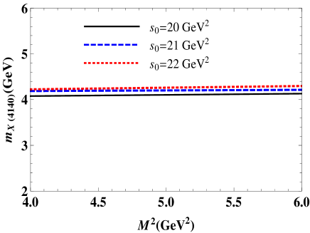
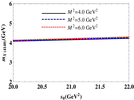
Figure 1: The mass of the $X(4140)$ state as a function of the Borel parameter $M^{2}$ at fixed $s_{0}$ (left panel), and as a function of the continuum threshold $s_{0}$ at fixed $M^{2}$ (right panel).

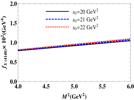
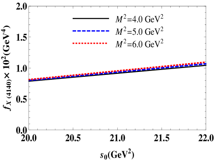
Figure 2: The dependence of the meson-current coupling $f_{X}$ of the $X(4140)$ resonance on the Borel parameter at chosen values of $s_{0}$ (left panel), and on the $s_{0}$ at fixed $M^{2}$ (right panel).

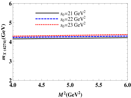
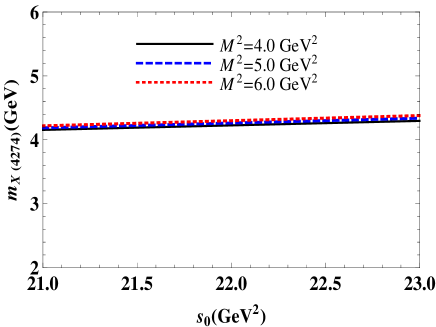
Figure 3: The mass of the $X(4274)$ resonance as a function of the Borel parameter $M^{2}$ at fixed $s_{0}$ (left panel), and as a function of the continuum threshold $s_{0}$ at fixed $M^{2}$ (right panel).

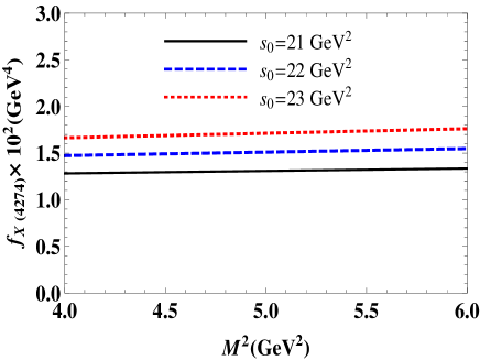
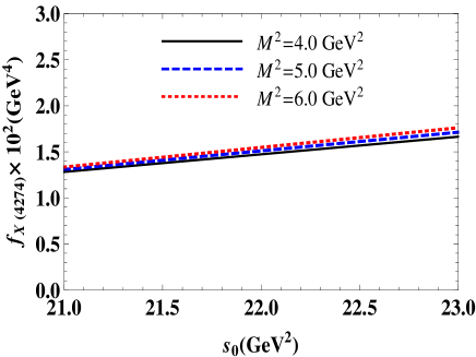
Figure 4: The meson-current coupling $f_{X}$ of the $X(4140)$ resonance as a function of the Borel parameter $M^{2}$ at chosen values of $s_{0}$ (left panel), and as a function of $s_{0}$ at fixed $M^{2}$ (right panel).

$X$	$X(4140)$	$X(4274)$
$M^{2}~{}(\mathrm{GeV}^{2}$)	$4-6$	$4-6$
$s_{0}~{}(\mathrm{GeV}^{2}$)	$20-22$	$21-23$
$m_{X}~{}(\mathrm{MeV})$	$4183\pm 115$	$4264\pm 117$
$f_{X}~{}(\mathrm{GeV}^{4})$	$(0.94\pm 0.16)\cdot 10^{-2}$	$(1.51\pm 0.21)\cdot 10^{-2}$

Table 2: The masses and meson-current couplings of the $X(4140)$ and $X(4274)$ tetraquarks.

The methods for deriving of the spectral density $\rho^{\mathrm{QCD}}(s)$ were presented in the literature (see, for example, Ref. Agaev:2016dev . Therefore, we do not concentrate here on details of these standard and rather routine calculations.

The expressions for the mass and meson-current coupling given by Eqs. (12) and (13) contain the input parameters, numerical values of which are collected in Table 1. The sum rules depend also on the auxiliary parameters $M^{2}$ and $s_{0}$. In general, physical quantities extracted from the sum rules should not depend on the Borel parameter and continuum threshold, but in real calculations we can only minimize their effect on obtained results. They have also to obey the standard requirements imposed by the sum rule calculations. Thus, in the working regions of these parameters a prevalence of the pole contribution to the sum rules and convergence of the operator product expansion (OPE) have to be satisfied. Namely these restrictions, and a stability of the obtained predictions determine ranges within of which the parameters $M^{2}$ and $s_{0}$ can be varied. Results of our analysis are collected in Table 2, where we provide both the working windows for the parameters $M^{2}$ and $s_{0}$, as well as, the sum rule’s results for the mass and meson-current couplings of the $X(4140)$ and $X(4274)$ resonances. In the working ranges of the parameters the pole contributions equal to $23\%$ of the whole results, which are typical for the sum rule calculations involving four-quark systems. In order to control the convergence of OPE we evaluate the contribution arising from each term of the fixed dimension: in the ranges shown in Table 2 convergence of OPE is fulfilled: It is enough to note that contribution of the dimension-$8$ term to the final result does not exceed $1\%$ of its value.

As is seen from Figs. 1 and 2, the mass and meson-current coupling of the $X(4140)$ state are sensitive to the parameters $M^{2}$ and $s_{0}$: While their effects on the mass $m_{X}$ are mild, the dependence of the meson-current coupling $f_{X}$ on the chosen values of the Borel and continuum threshold parameters is noticeable. These effects combined with ambiguities of the input parameters generate the theoretical errors in the sum rule calculations, which are their unavoidable feature. The errors of the calculations are also presented in Table 2. The similar estimations are valid for the $X(4274)$ state, as well (see Figs. 3 and 4).

The masses of the $X(4140)$ and $X(4274)$ found in the present work, are in a nice agreement with LHCb data. At this stage of our investigations we can conclude that $X(4140)$ and $X(4274)$ are the diquark-antidiquark $J^{PC}=1^{++}$ states of the color triplet and sextet multiplets, respectively.

III Width of $X(4140)\rightarrow J/\psi\phi$  and $X(4274)\rightarrow J/\psi\phi$ decays

The $X_{1}$ and $X_{2}$   states were observed as resonances in the $J/\psi\phi$ invariant mass distribution. Therefore, processes $X_{1}\rightarrow J/\psi\phi$ and $X_{2}\rightarrow J/\psi\phi$ may be considered as their main decays channels. In this section we are going to concentrate namely on these two decay processes. We will outline steps necessary to analyze the vertex $XJ/\psi\phi$, where $X$ is one of the $X_{1}$ and $X_{2}$ states, and calculate the strong coupling $g_{XJ/\psi\phi}$ and width of the decay $X\to J/\psi\phi$.

Within the sum rule method the strong vertex $XJ/\psi\phi$ can be studied using the correlation function

$$\Pi_{\mu\nu}(p,q)=i\int d^{4}xe^{ipx}\langle\phi(q)|\mathcal{T}\{J_{\mu}^{J/\psi}(x)J_{\nu}^{{\dagger}}(0)\}|0\rangle,$$ (14)

where $J_{\nu}$ and $J_{\mu}^{J/\psi}$ are the interpolating currents of the $X$ state and $J/\psi$ meson, respectively. The current $J_{\nu}$ is defined by one of Eqs. (3) and (4), whereas $J/\psi$ has the form

$$J_{\mu}^{J/\psi}(x)=\overline{c}_{l}(x)\gamma_{\mu}c_{l}(x).$$ (15)

We calculate $\Pi_{\mu\nu}(p,q)$ employing QCD sum rule on the light-cone and soft approximation. To this end, at first stage of calculations one has to express this function in terms of the physical quantities, namely in terms of the masses, decay constants of involved particles, and strong coupling $g_{XJ/\psi\phi}$ itself. For $\Pi_{\mu\nu}^{\mathrm{Phys}}(p,q)$ we get

$$\Pi_{\mu\nu}^{\mathrm{Phys}}(p,q) = \frac{\langle 0|J_{\mu}^{J/\psi}|J/\psi\left(p\right)\rangle}{p^{2}-m_{J/\psi}^{2}}\langle J/\psi\left(p\right)\phi(q)|X(p^{\prime})\rangle$$ (16)

$$\times\frac{\langle X(p^{\prime})|J_{\nu}^{\dagger}|0\rangle}{p^{\prime 2}-m_{X}^{2}}+\ldots,$$

where $p$, $q$ are the momenta of the $J/\psi$ and $\phi$ mesons, respectively, and by $p^{\prime}=p+q$ we denote the momentum of the $X$ state.

We define the matrix element of the $J/\psi$ meson in the form

$$\langle 0|J_{\mu}^{J/\psi}|J/\psi\left(p\right)\rangle=f_{J/\psi}m_{J/\psi}\varepsilon_{\mu}(p),$$

where $m_{J/\psi}$, $f_{J/\psi}$ and $\varepsilon_{\mu}(p)$ are its mass, decay constant and polarization vector, respectively. We introduce also the matrix element corresponding to the vertex

$$\langle J/\psi\left(p\right)\phi(q)|X(p^{\prime})\rangle$$

$$=ig_{XJ/\psi\phi}\epsilon_{\alpha\beta\gamma\delta}\varepsilon_{\alpha}^{\ast}(p)\varepsilon_{\beta}(p^{\prime})\varepsilon_{\gamma}^{\ast}(q)p_{\delta}.$$ (17)

Here $\varepsilon_{\gamma}^{\ast}(q)$ is the polarization vector of the $\phi$ meson. Then the contribution coming from the ground state takes the form

$$\Pi_{\mu\nu}^{\mathrm{Phys}}(p,q)=i\frac{f_{J/\psi}f_{X}m_{J/\psi}m_{X}g_{XJ/\psi\phi}}{\left(p^{\prime 2}-m_{X}^{2}\right)\left(p^{2}-m_{J/\psi}^{2}\right)}$$

$$\times\left(\epsilon_{\mu\nu\gamma\delta}\varepsilon_{\gamma}^{\ast}(p)p_{\delta}-\frac{1}{m_{X}^{2}}\epsilon_{\mu\beta\gamma\delta}\varepsilon_{\gamma}^{\ast}(p)p_{\delta}p_{\beta}^{\prime}p_{\nu}^{\prime}\right)+\ldots$$

In the soft limit $p=p^{\prime}$ (see, a discussion below and Ref. Agaev:2016dev ), and only the term $\sim i\epsilon_{\mu\nu\gamma\delta}\varepsilon_{\gamma}^{\ast}(p)p_{\delta}$ survives in Eq. (LABEL:eq:CorrF5).

In the soft-meson approximation we employ the one-variable Borel transformation on $p^{2}$. Then, an invariant amplitude $\Pi^{\mathrm{Phys}}(p^{2})$ depends on the variable $p^{2}$

$$\Pi^{\mathrm{Phys}}(p^{2})=\frac{f_{J/\psi}f_{X}m_{J/\psi}m_{X}g_{XJ/\psi\phi}}{\left(p^{2}-m^{2}\right)^{2}},$$ (19)

where $m^{2}=(m_{X}^{2}+m_{J/\psi}^{2})/2$. Additionally, we apply to both sides of the sum rule the operator

$$\left(1-M^{2}\frac{d}{dM^{2}}\right)M^{2}e^{m^{2}/M^{2}},$$ (20)

which eliminates effects of unsuppressed terms in $\Pi^{\mathrm{Phys}}(p^{2})$ appeared in the soft limit Ioffe:1983ju ; Braun:1995 .

The QCD expression for the correlation function $\Pi_{\mu\nu}^{\mathrm{QCD}}(p,q)$ is calculated employing the quark propagators. For the current $J_{\mu}^{1}$ it takes the following form

$$\Pi_{\mu\nu}^{\mathrm{QCD}}(p,q)=i\int d^{4}xe^{ipx}\epsilon^{ijk}\epsilon^{imn}$$

$$\times\left\{\left[\gamma_{\nu}\widetilde{S}_{c}^{ak}(x)\gamma_{\mu}\widetilde{S}_{c}^{na}(-x){}\gamma_{5}\right]\right.$$

$$\left.-\left[\gamma_{5}\widetilde{S}_{c}^{ak}(x){}\gamma_{\mu}\widetilde{S}_{c}^{na}(-x){}\gamma_{\nu}\right]\right\}_{\alpha\beta}\langle\phi(q)|\overline{s}_{\alpha}^{j}s_{\beta}^{m}|0\rangle,$$ (21)

with $\alpha$ and $\beta$ being the spinor indices.

To proceed we employ the replacement

$$\overline{s}_{\alpha}^{j}s_{\beta}^{m}\rightarrow\frac{1}{4}\Gamma_{\beta\alpha}^{k}\left(\overline{s}^{j}\Gamma^{k}s^{m}\right),$$ (22)

where $\Gamma^{k}$ is the full set of Dirac matrices, and carry out the color summation. Then we substitute Eq. (LABEL:eq:Qprop) into the expression obtained after the color summation and perform four dimensional integration over $x$. This integration leads to appearance of the Dirac delta $\delta^{4}(p^{\prime}-p)$ in the integrand. The correlation function does not contain the $s$-quark propagator, therefore the argument of the Dirac delta depends only on the four-momenta of the $X$ state and $J/\psi$ meson. The next operation, i.e. an integration over $p$ or $p^{\prime}$ inevitably equates $p=p^{\prime}$, which is the result of the conservation of the four-momentum at the vertex $XJ/\psi\phi$. In other words, to conserve the four-momentum in the tetraquark-meson-meson vertex one should set $q=0$, which in the full LCSR is known as the soft-meson approximation Braun:1995 . At vertices of conventional mesons, in general $q\neq 0$, and only in the soft-meson approximation one sets $q$ equal to zero, whereas the tetraquark-meson-meson vertex can be treated in the context of the LCSR method only if $q=0$. Nevertheless, an important observation made in Ref. Braun:1995 is that, both the soft-meson approximation and full LCSR treatment of the ordinary mesons’ vertices lead for the strong couplings to very close numerical results.

In the soft limit only the matrix element

$$\langle 0|\overline{s}(0)\gamma_{\mu}s(0)|\phi(p,\lambda)\rangle=f_{\phi}m_{\phi}\epsilon_{\mu}^{(\lambda)},$$ (23)

of the $\phi$- meson contributes to the correlation function, where $m_{\phi}$ and $f_{\phi}$ are its mass and decay constant, respectively. The soft-meson limit reduces also possible Lorentz structures in $\Pi_{\mu\nu}^{\mathrm{QCD}}(p,q)$ to the term $\sim i\epsilon_{\mu\nu\gamma\delta}\varepsilon_{\gamma}^{\ast}(p)p_{\delta}$, which matches with the corresponding structure in $\Pi_{\mu\nu}^{\mathrm{Phys}}(p,q=0)$.

$X$	$X(4140)$	$X(4274)$
$M^{2}~{}(\mathrm{GeV}^{2}$)	$5-7$	$5-7$
$s_{0}~{}(\mathrm{GeV}^{2}$)	$20-22$	$21-23$
$g_{XJ/\psi\phi}$	$2.34\pm 0.89$	$3.41\pm 1.21$
$\Gamma(X\to J/\psi\phi)~{}(\mathrm{MeV})$	$80\pm 29$	$272\pm 81$

Table 3: The strong coupling $g_{XJ/\psi\phi}$ and decay width $\Gamma(X\to J/\psi\phi)$.

The relevant invariant amplitude can be written down as a dispersion integral in terms of the spectral density $\rho_{c}^{\mathrm{QCD}}(s)$. We omit details of calculations and provide the final expression for $\rho_{c}^{\mathrm{QCD}}(s)$, which read

$$\rho_{c}^{\mathrm{QCD}}(s)=\frac{f_{\phi}m_{\phi}m_{c}}{4}\left[\frac{\sqrt{s(s-4m_{c}^{2})}}{\pi^{2}s}+\digamma^{\mathrm{n.-pert.}}(s)\right].$$ (24)

The nonperturbative component of $\rho_{c}^{\mathrm{QCD}}(s)$, i.e. $\digamma^{\mathrm{n.-pert.}}(s)$ is given by the following formula

$$\digamma^{\mathrm{n.-pert.}}(s)=\Big{\langle}\frac{\alpha_{s}G^{2}}{\pi}\Big{\rangle}\int_{0}^{1}f_{1}(z,s)dz+\Big{\langle}g_{s}^{3}G^{3}\Big{\rangle}$$

$$\times\int_{0}^{1}f_{2}(z,s)dz+\Big{\langle}\frac{\alpha_{s}G^{2}}{\pi}\Big{\rangle}^{2}\int_{0}^{1}f_{3}(z,s)dz,$$ (25)

where the terms proportional to $\langle\alpha_{s}G^{2}/\pi\rangle$, $\langle g_{s}^{3}G^{3}\rangle$ and $\langle\alpha_{s}G^{2}/\pi\rangle^{2}$ are nonperturbative contributions to the spectral density and have four, six and eight dimensions, respectively. The explicit form of the functions $f_{1}(z,s),\ f_{2}(z,s)$ and $f_{3}(z,s)$ are:

$$f_{1}(z,s)=\frac{1}{18r^{2}}\left\{-\left(2+3r(3+2r)\right)\delta^{(1)}(s-\Phi)\right.$$

$$\left.+(1+2r)\left[m_{c}^{2}-sr\right]\delta^{(2)}(s-\Phi)\right\},$$ (26)

$$f_{2}(z,s)=\frac{(1-2z)}{2^{7}\cdot 9\pi^{2}r^{5}}\left\{2r\left[3r\left(1+rR\right)\delta^{(2)}(s-\Phi)\right.\right.$$

$$\left.+\left[3sr^{2}(1+r)-2m_{c}^{2}\left(1+rR\right)\right]\delta^{(3)}(s-\Phi)\right]+$$

$$+\left[s^{2}r^{4}-2sm_{c}^{2}r^{2}(1+r)+m_{c}^{4}(1+rR)\right]$$

$$\left.\times\delta^{(4)}(s-\Phi)\right\},$$ (27)

$$f_{3}(z,s)=\frac{m_{c}^{2}\pi^{2}}{2^{2}\cdot 3^{4}r^{2}}\left[\delta^{(4)}(s-\Phi)-s\delta^{(5)}(s-\Phi)\right],$$ (28)

where we introduce the short-hand notations

$$\ r=z(z-1),\ R=3+r,\ \ \Phi=\frac{m_{c}^{2}}{z(1-z)},$$ (29)

and $\ \delta^{(n)}(s-\Phi)$ is defined as

$$\delta^{(n)}(s-\Phi)=\frac{d^{n}}{ds^{n}}\delta(s-\Phi).$$ (30)

For the interpolating current $J_{\mu}^{2}$ we find

$$\Pi_{\mu\nu}^{\mathrm{QCD}}(p,q)=i\int d^{4}xe^{ipx}\left\{\left[\gamma_{\nu}\widetilde{S}_{c}^{ib}(x)\gamma_{\mu}\widetilde{S}_{c}^{ai}(-x){}\gamma_{5}\right.\right.$$

$$\left.-\gamma_{5}\widetilde{S}_{c}^{ib}(x){}\gamma_{\mu}\widetilde{S}_{c}^{ai}(-x){}\gamma_{\nu}\right]_{\alpha\beta}\langle\phi(q)|\overline{s}_{\alpha}^{a}s_{\beta}^{b}|0\rangle$$

$$+\left[\gamma_{\nu}\widetilde{S}_{c}^{ib}(x)\gamma_{\mu}\widetilde{S}_{c}^{bi}(-x){}\gamma_{5}-\gamma_{5}\widetilde{S}_{c}^{ib}(x){}\gamma_{\mu}\widetilde{S}_{c}^{bi}(-x){}\gamma_{\nu}\right]_{\alpha\beta}$$

$$\left.\times\langle\phi(q)|\overline{s}_{\alpha}^{a}s_{\beta}^{a}|0\rangle\right\},$$ (31)

The corresponding spectral density is

$$\rho_{c}^{(2)\mathrm{QCD}}(s)=2\rho_{c}^{(1)\mathrm{QCD}}(s),$$ (32)

where $\rho_{c}^{(1)\mathrm{QCD}}(s)$ is given by Eq. (24).

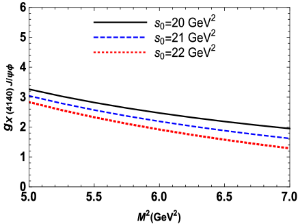
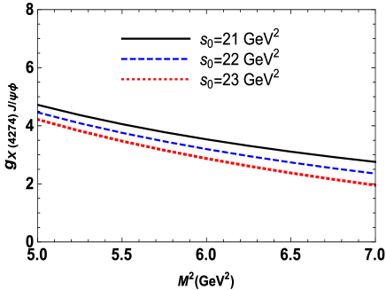
Figure 5: The strong coupling $g_{X_{1}J/\psi\phi}$ (left) and $g_{X_{2}J/\psi\phi}$ (right) as functions of the Borel parameter.

The final expression for the strong coupling $g_{XJ/\psi\phi}$ has the form

$$g_{XJ/\psi\phi} = \frac{1}{f_{J/\psi}f_{X}m_{J/\psi}m_{X}}\left(1-M^{2}\frac{d}{dM^{2}}\right)M^{2}$$ (33)

$$\times\int_{4m_{c}^{2}}^{s_{0}}dse^{(m^{2}-s)/M^{2}}\rho_{c}^{\mathrm{QCD}}(s).$$

The width of the decay $X\rightarrow J/\psi\phi$ is given by the formula

$$\Gamma(X\rightarrow J/\psi\phi)=\frac{\lambda(m_{X},m_{J/\psi},m_{\phi})}{48\pi m_{X}^{4}m_{\phi}^{2}}g_{XJ/\psi\phi}^{2}\left[\left(m_{X}^{2}+m_{\phi}^{2}\right)\right.$$

$$\times m_{J/\psi}^{4}+\left(m_{X}^{2}-m_{\phi}^{2}\right)^{2}\left(m_{X}^{2}+m_{\phi}^{2}-2m_{J/\psi}^{2}\right)$$

$$\left.+4m_{X}^{2}m_{J/\psi}^{2}m_{\phi}^{2}\right],$$ (34)

where $\lambda(a,b,c)$ is the standard function

$$\lambda(a,b,c)=\frac{\sqrt{a^{4}+b^{4}+c^{4}-2(a^{2}b^{2}+a^{2}c^{2}+b^{2}c^{2})}}{2a}.$$

The results of the numerical computations for the strong couplings and decay widths are collected in Table 3. Here we also show the working ranges for the parameters $M^{2}$ and $s_{0}$, where the predictions for the couplings $g_{X_{1}J/\psi\phi}$ and $g_{X_{2}J/\psi\phi}$ are obtained. Within these ranges the sum rules satisfy all requirements typical for such kind of calculations. Indeed, the pole contribution to the sum rule on the average amounts to $\sim 44\%$ of the result. The convergence of OPE is fulfilled, too. Thus dimension-8 contribution constitutes only $1\%$ of the sum rule.

In Fig. 5 we plot the couplings $g_{X_{1}J/\psi\phi}$ and $g_{X_{2}J/\psi\phi}$ as functions of the Borel parameter at fixed $s_{0}$. One can see that the couplings are sensitive to the choice of the auxiliary parameters $M^{2}$ and $s_{0}$. This sensitivity is a main source of theoretical ambiguities of the performed analysis, numerical estimates of which can be found in Table 3, as well.

Comparing theoretical predictions and LHCb data, one sees that width of the decay $X(4140)\to J/\psi\phi$ is in accord with the experimental data, whereas $\Gamma(X(4274)\to J/\psi\phi)$ considerably exceeds and does not explain them.

IV Discussion and concluding remarks

In the present work we have calculated the masses of the resonances $X(4140)$ and $X(4274)$, and width of the decay channels $X(4140)\to J/\psi\phi$ and $X(4274)\to J/\psi\phi$. We have treated these resonances as the $1^{++}$ states in the multiplet of the color triplet and sextet diquark-antidiquarks, respectively. As is seen from Table 4, our predictions for the masses of $X(4140)$ and $X(4274)$, obtained using the two-point QCD sum rule method, are in a nice agreement with recent measurements of the LHCb Collaboration Aaij:2016iza .

The $X(4140)$ and $X(4274)$ states were previously studied in Refs. Albuquerque:2009ak ; Chen:2010ze ; Chen:2016oma ; Wang:2016tzr ; Wang:2016dcb . Thus, the resonance $X(4140)$ was treated in Ref. Albuquerque:2009ak as a molecule-like bound state with $J^{PC}=0^{++}$ built of the mesons $D_{s}^{*}\bar{D}_{s}^{*}$. Calculation of its mass, performed there using two-point QCD sum rule method and relevant interpolating current gives a result, which correctly describes the experimental data. Nevertheless, the LHCb Collaboration have excluded interpretation of the $X(4140)$ resonance as a molecule-like state.

As we have noted above, the masses of the $X(4140)$ and $X(4274)$ resonances in the context of the two-point sum rule method were computed also in Ref. Chen:2010ze . The obtained predictions within errors explain the LHCb data Chen:2016oma . Let us note that $X(4140)$ and $X(4274)$ resonances were treated in Refs. Chen:2010ze ; Chen:2016oma as the axial-vector states with triplet and sextet color structures, respectively.

The investigations carried out in Ref. Wang:2016tzr using sum rule approach and two types of interpolating currents, however excluded interpretation of the $X(4140)$ resonance as a diquark-antidiquark state. The reason was that $m_{X_{1}}$ extracted from the corresponding sum rules either lay below LHCb data or overshot it (see, Table 4).

The $X(4274)$ was explored as a molecule-like color octet state Wang:2016dcb , and its mass $m_{X_{2}}$ was estimated as

$$m_{X_{2}}=4.27\pm 0.09\ \mathrm{GeV}.$$ (35)

But width of the decay $X(4274)\to J/\psi\phi$

$$\Gamma(X(4274)\to J/\psi\phi)=1.8\ \mathrm{GeV}$$ (36)

evaluated in the framework of the three-point QCD sum rule approach, considerably exceeded the LHCb value, therefore the author ruled out the suggested interpretation of the $X(4274)$ state.

We have calculated the widths of $X(4140/4274)\to J/\psi\phi$ decays, as well. The obtained predictions are collected in Table 4. It is evident, that our results for the mass and width of the $X(4140)$ resonance allow us to consider it as a serious candidate to the color triplet $J^{PC}=1^{++}$ diquark-antidiquark state. At the same time, interpretation of $X(4274)$ as a pure color sextet tetraquark which is, in accordance with our results, a ”wide” resonance, in the light of the LHCb data seems problematic: LHCb specifies it as a narrow state. Perhaps $X(4274)$ is an admixture of the color sextet tetraquark and a conventional charmonium. But this and alternative suggestions on the nature of the $X(4274)$ resonance require further investigations.

	$m_{X_{1}}$	$\Gamma_{X_{1}}$	$m_{X_{2}}$	$\Gamma_{X_{2}}$
	$(\mathrm{MeV})$	$(\mathrm{MeV})$	$(\mathrm{MeV})$	$(\mathrm{MeV})$
LHCb	$4146\pm 4.5_{-2.8}^{+4.6}$	$83\pm 21_{-14}^{+21}$	$4273\pm 8.3_{-3.6}^{+17.2}$	$56\pm 11_{-11}^{+8}$
Our w.	$4183\pm 115$	$80\pm 29$	$4264\pm 117$	$272\pm 81$
Albuquerque:2009ak	$4140\pm 90$	$-$	$-$	$-$
Chen:2010ze	$4070\pm 100$	$-$	$4220\pm 100$	$-$
Wang:2016tzr	$3950\pm 90$	$-$	$-$	$-$
	$5000\pm 100$	$-$	$-$	$-$
Wang:2016dcb	$-$	$-$	$4270\pm 90$	$1800$

Table 4: The LHCb data and theoretical predictions for the mass and decay width of the resonances $X(4140)$ and $X(4274)$.

Appendix A The $s$ and $c$-quark propagators

The light and heavy quark propagators are the important quantities to find QCD side of the correlation functions in both the mass and strong coupling calculations. We employ the $s$- quark propagator $S_{s}^{ab}(x)$, which is given by the following formula

$$S_{s}^{ab}(x)=i\delta_{ab}\frac{\not{x}}{2\pi^{2}x^{4}}-\delta_{ab}\frac{m_{s}}{4\pi^{2}x^{2}}-\delta_{ab}\frac{\langle\overline{s}s\rangle}{12}$$

$$+i\delta_{ab}\frac{\not{x}m_{s}\langle\overline{s}s\rangle}{48}-\delta_{ab}\frac{x^{2}}{192}\langle\overline{s}g_{s}\sigma Gs\rangle+i\delta_{ab}\frac{x^{2}\not{x}m_{s}}{1152}$$

$$\times\langle\overline{s}g_{s}\sigma Gs\rangle-i\frac{g_{s}G_{ab}^{\alpha\beta}}{32\pi^{2}x^{2}}\left[\not{x}{\sigma_{\alpha\beta}+\sigma_{\alpha\beta}}\not{x}\right]$$

$$-i\delta_{ab}\frac{x^{2}\not{x}g_{s}^{2}\langle\overline{s}s\rangle^{2}}{7776}-\delta_{ab}\frac{x^{4}\langle\overline{s}s\rangle\langle g_{s}^{2}G^{2}\rangle}{27648}+\ldots$$ (A.37)

For the $c$-quark propagator $S_{c}^{ab}(x)$ we employ the well-known expression

$$S_{c}^{ab}(x)=i\int\frac{d^{4}k}{(2\pi)^{4}}e^{-ikx}\Bigg{\{}\frac{\delta_{ab}\left({\not{k}}+m_{c}\right)}{k^{2}-m_{c}^{2}}$$

$$-\frac{g_{s}G_{ab}^{\alpha\beta}}{4}\frac{\sigma_{\alpha\beta}\left({\not{k}}+m_{c}\right)+\left({\not{k}}+m_{c}\right)\sigma_{\alpha\beta}}{(k^{2}-m_{c}^{2})^{2}}$$

$$+\frac{g_{s}^{2}G^{2}}{12}\delta_{ab}m_{c}\frac{k^{2}+m_{c}{\not{k}}}{(k^{2}-m_{c}^{2})^{4}}+\frac{g_{s}^{3}G^{3}}{48}\delta_{ab}\frac{\left({\not{k}}+m_{c}\right)}{(k^{2}-m_{c}^{2})^{6}}$$

$$\times\left[{\not{k}}\left(k^{2}-3m_{c}^{2}\right)+2m_{c}\left(2k^{2}-m_{c}^{2}\right)\right]\left({\not{k}}+m_{c}\right)+\ldots\Bigg{\}}.$$

In Eqs. (A.37) and (LABEL:eq:Qprop) we adopt the notations

$$G_{ab}^{\alpha\beta}=G_{A}^{\alpha\beta}t_{ab}^{A},\,\,~{}~{}G^{2}=G_{\alpha\beta}^{A}G_{\alpha\beta}^{A},$$

$$G^{3}=\,\,f^{ABC}G_{\mu\nu}^{A}G_{\nu\delta}^{B}G_{\delta\mu}^{C},$$ (A.39)

with $a,\,b=1,2,3$ being the color indices, and $A,B,C=1,\,2\,\ldots 8$  . In Eq. (A.39), $t^{A}=\lambda^{A}/2$, $\lambda^{A}$ are the Gell-Mann matrices, and the gluon field strength tensor $G_{\alpha\beta}^{A}\equiv G_{\alpha\beta}^{A}(0)$ is fixed at $x=0$.

References

• (1) R. Aaij et al. [LHCb Collaboration], Phys. Rev. Lett. 118, 022003 (2017); R. Aaij et al. [LHCb Collaboration], Phys. Rev. D 95, 012002 (2017).
• (2) T. Aaltonen et al. [CDF Collaboration], Phys. Rev. Lett. 102, 242002 (2009).
• (3) S. Chatrchyan et al. [CMS Collaboration], Phys. Lett. B 734, 261 (2014).
• (4) V. M. Abazov et al. [D0 Collaboration], Phys. Rev. D 89, 012004 (2014).
• (5) M. Gell-Mann, Phys. Lett. 8, 214 (1964).
• (6) R. L. Jaffe, Phys. Rev. D 15, 281 (1977).
• (7) E. Witten, Nucl. Phys. B 160, 57 (1979).
• (8) I. I. Balitsky, D. Diakonov and A. V. Yung, Phys. Lett. B 112, 71 (1982); Z. Phys. C 33, 265 (1986).
• (9) J. Govaerts, L. J. Reinders, H. R. Rubinstein and J. Weyers, Nucl. Phys. B 258, 215 (1985);J. Govaerts, L. J. Reinders and J. Weyers, Nucl. Phys. B 262, 575 (1985).
• (10) V. M. Braun and A. V. Kolesnichenko, Phys. Lett. B 175, 485 (1986) [Sov. J. Nucl. Phys. 44, 489 (1986)] [Yad. Fiz. 44, 756 (1986)].
• (11) V. M. Braun and Y. M. Shabelski, Sov. J. Nucl. Phys. 50, 306 (1989) [Yad. Fiz. 50, 493 (1989)].
• (12) R. Jaffe and F. Wilczek, Eur. Phys. J. C 33, S38 (2004).
• (13) R. L. Jaffe, Phys. Rept.  409, 1 (2005).
• (14) L. Maiani, F. Piccinini, A. D. Polosa and V. Riquer, Phys. Rev. D 71, 014028 (2005).
• (15) X. Liu, Z. G. Luo, Y. R. Liu and S. L. Zhu, Eur. Phys. J. C 61, 411 (2009).
• (16) Z. G. Wang, Eur. Phys. J. C 63, 115 (2009).
• (17) R. M. Albuquerque, M. E. Bracco and M. Nielsen, Phys. Lett. B 678, 186 (2009).
• (18) Z. G. Wang, Z. C. Liu and X. H. Zhang, Eur. Phys. J. C 64, 373 (2009).
• (19) Z. G. Wang, Int. J. Mod. Phys. A 26, 4929 (2011).
• (20) X. Liu, Z. G. Luo and S. L. Zhu, Phys. Lett. B 699, 341 (2011,) Erratum: [Phys. Lett. B 707, 577 (2012)].
• (21) J. He and X. Liu, Eur. Phys. J. C 72, 1986 (2012).
• (22) S. I. Finazzo, M. Nielsen and X. Liu, Phys. Lett. B 701, 101 (2011).
• (23) C. Hidalgo-Duque, J. Nieves and M. P. Valderrama, Phys. Rev. D 87, 076006 (2013).
• (24) F. Stancu, J. Phys. G 37, 075017 (2010).
• (25) S. Patel, M. Shah and P. C. Vinodkumar, Eur. Phys. J. A 50, 131 (2014).
• (26) R. Molina and E. Oset, Phys. Rev. D 80, 114013 (2009).
• (27) T. Branz, R. Molina and E. Oset, Phys. Rev. D 83, 114015 (2011).
• (28) I. V. Danilkin and Y. A. Simonov, Phys. Rev. D 81, 074027 (2010).
• (29) A. Esposito, A. Pilloni and A. D. Polosa, Phys. Rept.  668, 1 (2017).
• (30) V. Bhardwaj et al. [Belle Collaboration], Phys. Rev. D 93, 052016 (2016).
• (31) B. Aubert et al. [BaBar Collaboration], Phys. Rev. D 77, 111102 (2008).
• (32) D. Y. Chen, Eur. Phys. J. C 76, 671 (2016).
• (33) X. H. Liu, Phys. Lett. B 766, 117 (2017).
• (34) W. Chen and S. L. Zhu, Phys. Rev. D 83, 034010 (2011).
• (35) H. X. Chen, E. L. Cui, W. Chen, X. Liu and S. L. Zhu, Eur. Phys. J. C 77, 160 (2017).
• (36) Z. G. Wang, Eur. Phys. J. C 76, 657 (2016).
• (37) Z. G. Wang, Eur. Phys. J. C 77, 174 (2017).
• (38) Z. G. Wang, Eur. Phys. J. C 77, 78 (2017).
• (39) K. Abe et al. [Belle Collaboration], Phys. Rev. Lett. 94, 182002 (2005).
• (40) S. Uehara et al. [Belle Collaboration], Phys. Rev. Lett. 104, 092001 (2010).
• (41) B. Aubert et al. [BaBar Collaboration], Phys. Rev. Lett. 101 082001 (2008).
• (42) R. F. Lebed and A. D. Polosa, Phys. Rev. D 93, 094024 (2016).
• (43) F. Stancu, hep-ph/0607077.
• (44) L. Maiani, A. D. Polosa and V. Riquer, Phys. Rev. D 94, 054026, (2016).
• (45) R. Zhu, Phys. Rev. D 94, 054009 (2016).
• (46) M. A. Shifman, A. I. Vainshtein and V. I. Zhakharov, Nucl. Phys. B 147, 385 (1979).
• (47) I. I. Balitsky, V. M. Braun and A. V. Kolesnichenko, Nucl. Phys. B 312, 509 (1989).
• (48) B. L. Ioffe and A. V. Smilga, Nucl. Phys. B 232, 109 (1984).
• (49) V. M. Belyaev, V. M. Braun, A.  Khodjamirian and R. Rückl, Phys. Rev. D 51, 6177 (1995).
• (50) S. S. Agaev, K. Azizi and H. Sundu, Phys. Rev. D 93, 074002 (2016).
• (51) S. S. Agaev, K. Azizi and H. Sundu, Phys. Rev. D 93, 114007 (2016).
• (52) S. S. Agaev, K. Azizi and H. Sundu, Phys. Rev. D 93, 094006 (2016).
• (53) S. S. Agaev, K. Azizi and H. Sundu, Eur. Phys. J. Plus 131, 351 (2016).